The Finite Element Method for Stiff Ordinary Differential Equations

Abstract

The paper utilizes the continuous finite element method to solve stiff ordinary differential equations and proves that the linear finite element method and the quadratic finite element method have A-stability in solving autonomous ordinary differential equations, and exponential dichotomy in solving non-autonomous ordinary differential equations. In the numerical experiments of nonlinear autonomous and non-autonomous strongly and moderately stiff ordinary differential equations, a relatively large step size of $h=0.1$ was adopted over a longer period of time, with the numerical solution accuracy reaching ${10}^{-4}$. The superconvergence order maintained the theoretical order. A new approach is provided for solving stiff ordinary differential equations.

1. Introduction

Stiff equations are pervasive across numerous disciplines including aerospace engineering, chemical kinetics [1,2], physical systems modeling [3], biological processes, and multiscale engineering applications [4]. Such equations characterize systems in which multiple interacting sub-processes evolve at vastly disparate rates. Consequently, when solving these ordinary differential equations, one must account simultaneously for both rapidly and slowly varying components. This timescale nature poses substantial challenges and renders the solution procedure particularly demanding. Accordingly, the investigation of numerical methods for stiff equations carries considerable theoretical and practical importance.

A number of researchers have proposed various methods for the solution of stiff differential equations. Unconditionally stable implicit time-stepping schemes are currently the better choice. Frank R et al. adopted the fully implicit Runge–Kutta method for two classes of problems exhibiting order reduction phenomena in nonlinear stiff systems. The orders of all stages of fully implicit Runge–Kutta methods normally coincide with the numbers of stages [5]. Abd Rasid et al. proposed a new alternative implicit diagonal block backward differentiation formula (BBDF) approach for linear and nonlinear first-order stiff ordinary differential equations [6]. Junaidi SA et al. derived a composite backward differentiation formula (BDF) for stiff ordinary differential equations with given initial conditions by combining the implicit Euler and second-order Backward Differentiation Formula (BDF) with interpolation on intermediate solutions [7]. Shampine L.F. et al. proposed the IRKC code for the time integration of diffusion–reaction PDE systems, based on implicit–explicit Runge–Kutta–Chebyshev methods [8]. Cardone A et al. proposed a spatially and temporally adapted numerical solution for Boussinesq-type advection–diffusion problems, combining exponentially fitted finite differences (spatial) and an adaptive IMEX method (temporal) [9]. Xiao A et al. developed two IMEX multistep methods to reduce the computational cost of initial value problems for nonlinear ODEs with stiff and non-stiff terms, using implicit discretization for stiff terms and explicit for non-stiff ones [10]. Selvakumar K. et al. proposed a second-order, modified mid-point rule for stiff differential equations, which is an A-stable and L-stable finite difference method [11]. Rufai M A et al. proposed an efficient hybrid Nyström method (HNM) with optimized points and variable step size for solving Hamiltonian and stiff problems [12]. Ramos H et al. [13] introduced a new one-step method with three intermediate points for stiff differential systems, constructed using interpolation and collocation. The method adopts an embedded strategy for variable step size. Calvo M. et al. developed Singly TASE operators and modified Singly-RKTASE (MSRKTASE) methods for stiff differential equations, which offer improved efficiency, accuracy, stability and low storage [14,15].

The majority of existing methods for stiff problems are focused on finite difference methods, which are based on Taylor expansions and have relatively high requirements for the regularity of the solution. The finite element method [16,17] is another widely adopted numerical technique for solving differential equations. After decades of development, the finite element methodology possesses a mature theoretical foundation and enjoys broad application [18,19]. Hulbert G M et al. [20] proposed a time-discontinuous Galerkin finite element method with least-squares stabilizing terms for structural dynamics equations, proving its convergence in a norm stronger than the energy norm. The method achieves better accuracy and stability under specific temporal interpolations. The continuous finite element method can also achieve good solution results in conservation-type differential equations, such as the Schrödinger equation [21,22]. Tang et al. proposed the continuous finite element method (COFEM) to solve Hamiltonian systems and proved that the linear and quadratic continuous finite element methods for ordinary differential equations yield second-order and third-order pseudo-symplectic schemes, respectively, while preserving energy; for linear Hamiltonian systems, the methods are both symplectic and energy conserving [23].

Based on the continuous finite element method through integration on both sides, with relatively weak requirements for the regularity of the solution, this paper employs this method to solve stiff ordinary differential equations. This method possesses A-stability and exponential dichotomy in autonomous and non-autonomous differential equations respectively. The error accuracy obtained by using COFEM for these two types of stiff differential equations over a long time interval can reach the theoretically expected convergence order, and can also achieve an accuracy of ${10}^{-4}$ when a larger step size is selected, providing a good approach for the numerical calculation of stiff differential equations.

2. Stiff ODEs and Finite Element Methods

2.1. Stiff ODEs

Definition 1.

If nonlinear differential equations

$$\left\{\begin{array}{cc}{y}^{\prime }\left(t\right)=f(t,y\left(t\right)),\hfill & t\in (0,T]\hfill \\ y\left(0\right)=y_0\in {\mathbb{R}}^d\hfill \end{array}\right.$$

(1)

where $y^{\prime }\left(t\right)$ is a function of t and y, $y=({\overline{y}}_1,\dots ,{\overline{y}}_d)$, and $f=({\overline{f}}_1,\dots ,{\overline{f}}_d)$. The eigenvalues ${\lambda }_i$ of the Jacobian matrix $J(t,y(t\left)\right)$

$$J(t,y\left(t\right))={\left[{\displaystyle \frac{\partial f_i}{\partial \overline{y_j}}}(t,y\left(t\right))\right]}_{i,j=1}^d$$

(2)

of the function f satisfy the condition

$$\begin{array}{c}\mathit{\left(}\mathsf{1}\mathit{\right)}Re{\lambda }_i<0,i=1,\dots ,d\hfill \\ \mathit{(}\mathsf{2}\mathit{)}R={\displaystyle \frac{{max}_{1\le i\le d}\left|Re{\lambda }_i\right|}{{min}_{1\le i\le d}\left|Re{\lambda }_i\right|}}\gg 1\hfill \end{array}$$

(3)

Then the differential equation is classified as stiff, and the ratio R is termed the stiffness ratio. The greater the value of R, the more severe the stiffness. In general, for a sufficiently large $R=O\left({10}^p\right),p\ge 1$, the equation is considered stiff.

2.2. Finite Element Methods

For (1), partition the interval $J=[0,T]$, $t_0=0<t_1<t_2<\dots <t_N=T$, denoting the element by $I_j=(t_{j-1},t_j)$, its midpoint is defined as ${\overline{t}}_j={\displaystyle \frac{t_{j-1}+t_j}{2}}$, step length by $h_j=t_j-t_{j-1}$ and the maximum step size by $h={max}_j{h}_j,j=1,2,\dots ,N$, on each subinterval, the finite element space of the vector y is defined, where each component of the vector is a continuous and piecewise m-th-order polynomial function

$$S^h=\left\{\omega {\left|\omega \in C\left(I;{\mathbb{R}}^d\right),\omega \right|}_{I_j}\in {\left(P_m\right)}^d,j=1,2,\dots ,N\right\}$$

(4)

$P_m$ is an m-th-degree polynomial, i.e., each component of the vector is a piecewise m-th-degree continuous polynomial.

Taking $\omega \in S^h$, its derivate ${\omega }^{\prime }$ is ${\left(P_{m-1}\right)}^d$. We can take test function $v={\omega }^{\prime }\in {\left(P_{m-1}\right)}^d$. Let the inner product norm be, respectively,

$$(f,v)={\int }_{I}fvdt$$

(5)

$$\parallel \mathbf{y}\parallel =\underset{1\le i\le d}{max}\left|\overline{y_i}\right|$$

(6)

The weak form on each subinterval $I_j$ is

$$\left(y^{\prime },v\right)={\int }_{I_j}f·vdt$$

(7)

We obtain the equation

$${\int }_{I_j}\left(y^{\prime }-f(t,y)\right)·vdt=0$$

(8)

The M-th order continuous finite element solution is $Y_h\in S^h$, noting Y is $Y_h$, and $Y=(\overline{Y_1},\dots ,\overline{Y_d})$ is defined on each element $I_j$ by the relation

$$\begin{array}{c}{\int }_{I_j}\left(Y^{\prime }-f(t,Y)\right)·vdt=0,Y\left(0\right)=y_0,v\in {\left(P_{m-1}\right)}^d,j=1,2,\dots ,N\hfill \end{array}$$

(9)

where the components of v are ${\left(t-t_{j-1}\right)}^i,i=0,1,\dots ,m-1$. In IVP, though each component of the element $Y\in S^h$ is an m-th-degree polynomial, $Y\left(t_{j-1}\right)$ is known, and there exists only an m-th order of freedom on the interval $I_j$. From $\left(6\right)$ we obtain a system of equations which determines the values of Y on $I_j$. Y at the nodal points $t_j$ is denoted as $Y\left(t_j\right)=Y_j$. Thus, Y can subsequently be defined on the interval $I_{j+1}$.

Lemma 1

([24]). The degree m continuous finite element solution $Y\in S^h$ for (1) has the best superconvergence at all nodes $t_j$:

$$\left({\overline{y}}_i-\overline{Y_i}\right)\left(t_j\right)=O\left(h^{2m}\right),i=1,\dots ,d,j=1,\dots ,N$$

(10)

From Lemma 1, the local truncation error of the linear finite element solution Y is of the order $O\left(h^2\right)$, and hence

$$∥(y-Y)\left(t_j\right)∥=O\left(h^2\right),j=1,\dots ,N$$

(11)

halve the step size, and with $h/2$ as the new step size, proceed in two steps from $t_{j-1}$ to $t_j,j=1,\dots ,N$ to compute another approximate solution $Y_{\frac{h}{2}}$. The local truncation error per step is $c{(h/2)}^2$, i.e.,

$$∥(y-Y_{\frac{h}{2}})\left(t_j\right)∥\approx c{\left({\displaystyle \frac{h}{2}}\right)}^2={\displaystyle \frac{c}{4}}{h}^2$$

(12)

From (11) and (12), we obtain

$$∥{\displaystyle \frac{\left(y-Y_{\frac{h}{2}}\right)\left(t_j\right)}{(y-Y)\left(t_j\right)}}∥\approx {\displaystyle \frac{1}{4}}$$

(13)

From this, we obtain the following estimation:

$$\begin{array}{c}∥\left(Y_{\frac{h}{2}}-Y\right)\left(t_j\right)∥\approx ∥(y-Y)\left(t_j\right)-\left(y-Y_{\frac{h}{2}}\right)\left(t_j\right)∥\approx {\displaystyle \frac{3c{h}^2}{4}}\hfill \end{array}$$

(14)

Combining (13) and (14) yields

$$∥(y-Y_{\frac{h}{2}})\left(t_j\right)∥\approx {\displaystyle \frac{1}{3}}∥\left(Y_{\frac{h}{2}}-Y\right)\left(t_j\right)∥$$

(15)

Therefore, when the analytical solution is unknown, the error of the linear element solution can be evaluated by examining the discrepancy between the numerical results obtained before and after halving the step size. A similar approach can be derived for the quadratic element:

$$∥(y-Y_{\frac{h}{2}})\left(t_j\right)∥\approx {\displaystyle \frac{1}{15}}∥\left(Y_{\frac{h}{2}}-Y\right)\left(t_j\right)∥$$

(16)

3. Stability Analysis

3.1. Autonomous Ordinary Differential Equation

Definition 2.

A numerical method applied to the model equation $y^{\prime }=\lambda y$ is called absolutely stable if the computed solution $y_{n+1}=E\left(h\lambda \right)y_n$ satisfies $\left|E\right(h\lambda \left)\right|<1$. In the complex plane, $\mu =h\lambda$ for the numerical method is stable, forming region with unconditional stability. Its intersection with the real axis is termed the interval of absolute stability.

Definition 3.

A numerical method is said to be A-stable if its region of absolute stability contains the entire left half of the complex plane, i.e.,

$$C_{-1}=\{h\lambda \mid Re\left(h\lambda \right)<0\}$$

(17)

Theorem 1.

The linear finite element method is absolutely stable and A-stable.

Proof. 

For the test equation $y^{\prime }=My$, $\lambda$ is a matrix of $d\times d$; applying the continuous finite element method on the interval $I_j=\left[t_{j-1},t_j\right]$, the m-th finite element $Y\in S^h$ satisfies

$${\int }_{I_j}{Y}^{\prime }·vdt={\int }_{I_j}MY·vdt,v\in {\left(P_{m-1}\right)}^d$$

(18)

On each element $I_j$, in the linear finite element method space,

$$\begin{array}{cc}\hfill S^h=\left\{\omega \right|\omega \in C\left(I;{\mathbb{R}}^d\right),& \omega \in {\left(P_1\right)}^d\mathrm{on}\mathrm{each}{I}_j,\hfill \\ \hfill & j=1,2,\dots ,N,P_1\mathrm{is}\mathrm{polynomials}\mathrm{of}\mathrm{degree}1\}\hfill \end{array}$$

(19)

Obtaining the finite element solution

$$Y={\displaystyle \frac{t_{j+1}-t}{h_j}}{Y}_j+{\displaystyle \frac{t-t_j}{h_j}}{Y}_{j+1}$$

(20)

Denote the step size as $h=h_j=t_j-t_{j-1}$. By performing a variable transformation $t={\displaystyle \frac{h}{2}}x+{\displaystyle \frac{t_{j-1}+t_j}{2}}$ on element $I_j$, map the integration interval to the standard reference interval $[-1,1]$.

By taking each component of v as 1 and denoting the linear element solution Y at node $t_j$ as $Y_j$, it yields

$$E\left(hM\right)={\left(I-{\displaystyle \frac{h}{2}}M\right)}^{-1}\left(I+{\displaystyle \frac{h}{2}}M\right).$$

(21)

For each $\lambda$, if eigenvalue $Re\left({\lambda }_i\right)<0,i=1,\dots ,d$ of M, $h>0$ we have

$$\left|E\left(hM\right)\right|=\left|{\displaystyle \frac{I+\frac{hM}{2}}{I-\frac{hM}{2}}}\right|<1$$

(22)

Hence, the linear finite element method is A-stable for positive step size h; its region of absolute stability consists of the entire left half-plane, with the interval $-\infty <h\lambda <0$ defining the interval of absolute stability.

For nonlinear differential equations $y^{\prime }=f\left(y\right)$, the conclusions of Theorem 1 can be extended through local linearization in the vicinity of an equilibrium point. Let $y^{*}\in {\mathbb{R}}^d$ be an equilibrium point so that $f\left(y^{*}\right)=0$. For any y in a sufficiently small neighborhood of $y^{*}$, the Taylor expansion of $f\left(y\right)$ about $y^{*}$ yields

$$f\left(y\right)=f\left(y^{*}\right)+A(y-y^{*})+R\left(y\right)$$

(23)

where $A\in {\mathbb{R}}^{d\times d}$ is the Jacobian matrix of f evaluated at $y^{*}$, and $R\left(y\right)=O(\parallel y-y^{*}{\parallel }^2)$ denotes the higher-order remainder term. Substituting $f\left(y^{*}\right)=0$ and defining the perturbation $\delta y=y-y^{*}$, we obtain

$$f\left(y\right)=A\delta y$$

(24)

this reduces to the linear form. □

Hence, Theorem 1 holds for nonlinear differential equations.

Theorem 2.

The quadratic finite element method is absolutely stable and A-stable.

Proof. 

For the test equation $y^{\prime }=My$ applying the continuous finite element method. On $I_j=\left(t_{j-1},t_j\right)$, $Y\in S^h$

$${\int }_{I_j}{Y}^{\prime }·vdt={\int }_{I_j}MY·vdt,v\in {\left(P_{m-1}\right)}^d$$

(25)

On each element $I_j$, the quadratic finite element method has

$$\begin{array}{cc}\hfill S^h=\{\omega \mid \omega \in C\left(I;{\mathbb{R}}^d\right),& \omega \in P_2\mathrm{on}\mathrm{each}{I}_j,\hfill \\ \hfill & j=1,2,\dots ,N,{\left(P_2\right)}^d\mathrm{is}\mathrm{polynomials}\mathrm{of}\mathrm{degree}2\}\hfill \end{array}$$

(26)

Obtaining the quadratic element solution

$$Y={\displaystyle \frac{\left(t-t_{j+\frac{1}{2}}\right)\left(t-t_{j+1}\right)}{{\left(h_j\right)}^2/2}}{Y}_j+{\displaystyle \frac{\left(t-t_{j+1}\right)\left(t-t_j\right)}{-{\left(h_j\right)}^2/4}}{Y}_{j+\frac{1}{2}}+{\displaystyle \frac{\left(t-t_{j+\frac{1}{2}}\right)\left(t-t_j\right)}{{\left(h_j\right)}^2/2}}{Y}_{j+1}$$

(27)

set each component of v to $1,t-t_j$, denoting the quadratic finite element solution Y at node $t_j$ as $Y_j$, yielding

$$\begin{array}{c}{\int }_{I_j}{Y}^{\prime }dt={\int }_{I_j}MYdt\hfill \\ {\int }_{I_j}{Y}^{\prime }\left(t-t_j\right)dt={\int }_{I_j}MY\left(t-t_j\right)dt\hfill \end{array}$$

(28)

Denote the step size as $h=h_j=t_j-t_{j-1}$. By performing a variable transformation $t={\displaystyle \frac{h}{2}}x+{\displaystyle \frac{t_{j-1}+t_j}{2}}$ on element $I_j$, map the integration interval to the standard reference interval $[-1,1]$. Let

$$C=\left(\begin{array}{cc}-{\displaystyle \frac{2}{3}}hM& I-{\displaystyle \frac{h}{6}}M\\ -{\displaystyle \frac{2}{3}}Ih-{\displaystyle \frac{h^2}{3}}M& {\displaystyle \frac{5}{6}}Ih-{\displaystyle \frac{h^2}{6}}M\end{array}\right)$$

(29)

since

$$det\left(C\right)={\left({\displaystyle \frac{h}{18}}\right)}^{d}det\left(M^2{h}^2-6Mh+12I\right)$$

(30)

Therefore, C is reversible if and only if

$$det\left(M^2{h}^2-6Mh+12I\right)\ne 0$$

(31)

The above equation is equivalent to

$$\prod _{i=1}^d\left({\lambda }_i^2{h}^2-6{\lambda }_{i}h+12\right)\ne 0$$

(32)

where ${\lambda }_i$ is an eigenvalue of M. Solving quadratic equations ${\lambda }_i^2{h}^2-6{\lambda }_{i}h+12=0$ for h, obtaining

$$h={\displaystyle \frac{6{\lambda }_i\pm \sqrt{36{\lambda }_i^2-48{\lambda }_i^2}}{2{\lambda }_i^2}}={\displaystyle \frac{6\pm \sqrt{-12}}{{\lambda }_i}}$$

(33)

For real negative eigenvalues, the determinant never vanishes for any positive step size $h>0$. Hence, C is invertible, and we obtain

$$\left({\displaystyle \genfrac{}{}{0pt}{}{y_{j-\frac{1}{2}}}{y_j}}\right)=\left({\displaystyle \genfrac{}{}{0pt}{}{\frac{-M^2{h}^2-24I}{2M^2{h}^2-12Mh+24I}{y}_{j-1}}{\frac{M^2{h}^2+6Mh+12I}{M^2{h}^2-6Mh+12I}{y}_{j-1}}}\right)$$

(34)

We obtain

$$y_j={\displaystyle \frac{M^2{h}^2+6Mh+12I}{M^2{h}^2-6Mh+12I}}{y}_{j-1}$$

(35)

Hence obtaining

$$E\left(hM\right)={\left({\left(hM\right)}^2-6\left(hM\right)+12I\right)}^{-1}\left({\left(hM\right)}^2+6\left(hM\right)+12I\right)$$

(36)

For each $\lambda$, if eigenvalue $Re\left({\lambda }_i\right)<0,i=1,\dots ,d$ of M, arbitrary $h>0$ we have

$$\left|E\left(h\lambda \right)\right|=\left|{\displaystyle \frac{M^2{h}^2+6Mh+12}{M^2{h}^2-6Mh+12}}\right|<1$$

(37)

Hence, the determinant is non-vanishing for any positive step size $h>0$ and for all ${\lambda }_i,i=1,\dots ,d$ with $Re{\lambda }_i<0$, the quadratic FEM is A-stable. Its region of absolute stability covers the entire left half-plane, with the interval $-\infty <h\lambda <0$ representing the interval of absolute stability. □

By the same token, Theorem 2 holds for nonlinear differential equations.

3.2. Non-Autonomous Ordinary Differential Equations

Consider the linear discrete non-autonomous equation

$$y_{n+1}=A\left(t_n\right)y_n$$

(38)

where $n\in J$, J on the interval $\mathbb{Z}$, and $A\left(t_n\right)$ is the $d\times d$ invertible matrix. For any $m,n\in J$ define the state transition matrix

$$\mathrm{\Phi }(n,m)=\left\{\begin{array}{cc}{A}_{n-1}·A_{n-2}·\dots ·A_m\hfill & n>m\\ I\hfill & n=m\\ A_n^{-1}·A_{n+1}^{-1}·\dots ·A_{m-1}^{-1}\hfill & n<m\end{array}\right.$$

(39)

Definition 4.

If there exists a family of projection operators $P_n$ (that is $P_n^2=P_n$) and constants $K>0,0<\lambda <1$ such that for any $m,n\in J$ all have

$$\mathrm{\Phi }(n,m)P_m=P_n\mathrm{\Phi }(m,n)$$

(40)

as well as

$$\begin{array}{c}∥\mathrm{\Phi }(n,m)P_m∥\le K{\lambda }^{n-m},m\le n\\ ∥\mathrm{\Phi }(n,m)\left(I-P_m\right)∥\le K{\lambda }^{m-n},n\le m\end{array}$$

(41)

Then Equation (38) is said to have exponential dichotomy. Here, K is the binary constant, and λ is the binary exponent.

Theorem 3.

The linear FEM for non-autonomous equations has exponential dichotomy.

Proof. 

Examine the overall linear non-autonomous differential equation system

$$y^{\prime }=A\left(t\right)y\left(t\right)t\in I=[0,T]$$

(42)

$A\left(t\right)\in {\mathbb{R}}^{d\times d}$ is the coefficient matrix. $y={\left(y_1\left(t\right),\dots ,y_d\left(t\right)\right)}^T$. Among them $\parallel A\left(t\right)\parallel \le L$.

Partition the interval $I=[0,T]$, $t_0=0<t_1<t_2<\dots <t_N=T$. Denote the element by $I_j=(t_{j-1},t_j)$. The midpoint is ${\overline{t}}_j={\displaystyle \frac{t_{j-1}+t_j}{2}}$, the step length is $h_j=t_j-t_{j-1}$, and the maximum step size is $h={max}_j{h}_j$. Based on this, the finite element space of the vector y is defined, where each component of the vector is a continuous and piecewise m-th-order polynomial function

$$S^h=\left\{\omega {\left|\omega \in C\left(I;{\mathbb{R}}^d\right),\omega \right|}_{I_j}\in {\left(P_m\right)}^d,j=1,2,\dots ,N\right\}$$

(43)

and $P_m$ is an m-th-degree polynomial, i.e., each component of the vector is a piecewise m-th-degree continuous polynomial. By the continuous finite element method, $y_h\in S^h$, and the m-th element on the interval $I_j=(t_{j-1},t_j)$ satisfies

$${\int }_{I_j}\left(y_h^{\prime },v\right)dt={\int }_{I_j}\left(A\left(t\right)y_h,v\right)dt,v\in P_{m-1}$$

(44)

In each element $I_j$, there is one finite element method:

$$S^h=\left\{\omega {\left|\omega \in C\left(I;{\mathbb{R}}^d\right),\omega \right|}_{I_j}\in {\left(P_1\right)}^d,j=1,2,\dots ,N\right\}$$

(45)

$P_1$ is a first-degree polynomial, and the finite element solution is $y_h\in S^h$. By taking each component of v as 1 and denoting the nodal values of the linear element solution $y_h$ at node $t_j$ as $y_j$, Equation $\left(44\right)$ yields

$$y_j-y_{j-1}={\displaystyle \frac{h}{2}}\left({\int }_{I_j}A\left(t\right)L_j\left(t\right)y_{j}dt+{\int }_{I_j}A\left(t\right)L_{j-1}\left(t\right)y_{j-1}dt\right)$$

(46)

Then

$$y_j={\left(I-{\displaystyle \frac{h{\int }_{I_j}A\left(t\right)L_j\left(t\right)dt}{2}}\right)}^{-1}\left(I+{\displaystyle \frac{h{\int }_{I_j}A\left(t\right)L_{j-1}\left(t\right)dt}{2}}\right)y_{j-1}.$$

(47)

Since $\parallel A\left(t\right)\parallel \le C$.

$$∥{\int }_{I_j}A\left(t\right)L_j\left(t\right)dt∥\le {\int }_{I_j}\parallel A\left(t\right)\parallel L_j\left(t\right)dt\le C{\int }_{I_j}{L}_j\left(t\right)dt=C{\displaystyle \frac{h}{2}}$$

(48)

From the matrix form of the Neumann series, if

$$∥{\displaystyle \frac{h{\int }_{I_j}A\left(t\right)L_j\left(t\right)dt}{2}}∥\le 1$$

(49)

then $I-{\displaystyle \frac{h{\int }_{I_j}A\left(t\right)L_j\left(t\right)dt}{2}}$ is reversible, so the sufficient condition is $h<{\displaystyle \frac{2}{\sqrt{C}}}$. Similarly, $h<{\displaystyle \frac{2}{\sqrt{C}}}$ is also a sufficient condition for $I+{\displaystyle \frac{h{\int }_{I_j}A\left(t\right)L_j\left(t\right)dt}{2}}$ to be invertible.

Let

$$B_j={\left(I-{\displaystyle \frac{h{\int }_{I_j}A\left(t\right)L_j\left(t\right)dt}{2}}\right)}^{-1}\left(I+{\displaystyle \frac{h{\int }_{I_j}A\left(t\right)L_{j-1}\left(t\right)dt}{2}}\right)$$

(50)

then

$$y_j=B_j{y}_{j-1}$$

(51)

when $h<{\displaystyle \frac{2}{\sqrt{C}}}$ occurs, $B_j$ is reversible.

Performing the Schur decomposition on $B_j$, we have

$$B_j=U_j{R}_j{U}_j^T$$

(52)

Among them, $U_j$ is an orthogonal matrix (satisfied $U_j^T{U}_j=I$). $R_j$ is a matrix in upper triangular form, where the diagonal entries correspond to the eigenvalues of $U_j$. Let ${\left\{u_i\left(j\right)\right\}}_{i=1}^d$ be the column vectors of $U_j$ and form an orthogonal basis.

Construct another set of orthogonal basis $\left\{w_i\left(j\right)\right\}$ as

$$w_i\left(j\right)=U_j{e}_i=u_i\left(j\right)$$

(53)

Under the Schur decomposition, the dual basis satisfies

$$⟨u_i\left(j\right),u_k\left(j\right)⟩={\delta }_{ik}$$

(54)

and taking $w_i\left(j\right)=u_i\left(j\right)$, there is $⟨u_i\left(j\right),w_k\left(j\right)⟩={\delta }_{ik}$, and the inner product is the Euclidean inner product.

Starting from $j=0$, by QR iteration, let $Q_0=U_0$. We have

$$B_j{Q}_j=Q_{j+1}{R}_j^{\prime }$$

(55)

Among them, $Q_j$ is an orthogonal matrix. $R_j^{\prime }$ is a matrix in upper triangular form. Approximated by the Lyapunov exponent as

$${\chi }_i\approx {\displaystyle \frac{1}{N}}\sum _{j=0}^{N-1}ln\left|{\left(R_j^{\prime }\right)}_{ii}\right|$$

(56)

Stabilize the direction: ${\chi }_i<0$. The unstable direction is ${\chi }_i>0$. Letting $Z_s=\left\{i:{\chi }_i<0\right\}$, $u_i\left(j\right)$ is the i-th column of $U_j$, and the stable subspace

$$S_j=span\left\{u_i\left(j\right);i\in Z_s\right\}$$

(57)

Projection operator $P_j:{\mathbb{R}}^d\to {\mathbb{R}}^d$:

$$P_j\left(x\right)=\sum _{i\in Z_s}⟨x,w_i\left(j\right)⟩u_i\left(j\right)\forall x\in {\mathbb{R}}^d$$

(58)

Since $w_i\left(j\right)=u_i\left(j\right)$, the matrix of the projection operator in the standard basis is

$$P_j\left(x\right)=\left[P_j\right]x=\sum _{i\in Z_s}⟨x,w_i\left(j\right)⟩u_i\left(j\right)$$

(59)

that is

$$\left[P_j\right]=\sum _{i\in Z_s}{u}_i\left(j\right)u_i{\left(j\right)}^T$$

(60)

Idempotence ($P_j^2=P_j$) is proved as follows: Since $\left[P_j\right]={\sum }_{i\in Z_s}{u}_i\left(j\right)u_i{\left(j\right)}^T$, ${\left\{u_i\left(j\right)\right\}}_{i\in Z_s}$ is an orthonormal vector group. Then

$$P_j^2=\left(\sum _{i\in Z_s}{u}_i\left(j\right)u_i{\left(j\right)}^T\right)\left(\sum _{i\in Z_s}{u}_i\left(j\right)u_i{\left(j\right)}^T\right)=\sum _{i\in Z_s}\sum _{k\in Z_s}{u}_i\left(j\right)u_i{\left(j\right)}^T{u}_k\left(j\right)u_k{\left(j\right)}^T=P_j$$

(61)

By orthogonality:

$$⟨u_i\left(j\right),u_k\left(j\right)⟩={\delta }_{ik}\left(i,k\in Z_s\right)$$

(62)

we have $P_j^2=P_j$.

The proof of commutativity ($\mathrm{\Phi }(n,m)P_m=P_n\mathrm{\Phi }(n,m)$) is as follows. From the QR iteration, we have

$$B_j{Q}_j=Q_{j+1}{R}_j^{\prime }$$

(63)

Partition $Q_j$ into stable and unstable blocks

$$Q_j=\left[V_j,W_j\right],V_j=\left[u_i\left(j\right)\mid i\in Z_s\right]\in {\mathbb{R}}^{n\times k},W_j=\left[u_i\left(j\right)\mid i\notin Z_s\right]\in {\mathbb{R}}^{n\times (n-k)}$$

(64)

then $P_j=V_j{V}_j^T,I-P_j=W_j{W}_j^T$.

When $n\ge m$, by mathematical induction, when $n=m$, $\mathrm{\Phi }(n,m)=I$, obviously there is $\mathrm{\Phi }(n,m)P_m=P_m=P_m\mathrm{\Phi }(n,m)$.

When $n=m+1$ to prove $\mathrm{\Phi }(n,m)P_m=P_n\mathrm{\Phi }(n,m)$ that is $B_m{P}_m=P_{m+1}{B}_m$.

Since

$$\begin{array}{cc}\hfill B_m{P}_m& =B_m{V}_m{V}_m^T\hfill \\ \hfill P_{m+1}{B}_m& =V_{m+1}{V}_{m+1}^T{B}_m\hfill \end{array}$$

(65)

From the QR iteration, we have

$$B_j{Q}_j=Q_{j+1}{R}_j^{\prime }$$

(66)

Block matrices are

$$B_m\left[V_m,W_m\right]=\left[V_{m+1},W_{m+1}\right]\left[\begin{array}{cc}{R}_{11}& R_{12}\\ 0& R_{22}\end{array}\right]$$

(67)

Here, $R_{11}$ is an $k\times k$ upper right triangular block. When the $QR$ iteration algorithm is applied to the Lyapunov exponent and sorted by the positive and negative values of ${\chi }_i$, if the stable and unstable subspaces are not coupled under the action of $B_j$, then $R_{12}=0$.

$$B_m{V}_m=V_{m+1}{R}_{11}+W_{m+1}·0=V_{m+1}{R}_{11}$$

(68)

then

$$B_m{P}_m=B_m{V}_m{V}_m^T=\left(V_{m+1}{R}_{11}\right)V_m^T$$

(69)

since

$$B_{m}I=B_m\left(V_m{V}_m^T+W_m{W}_m^T\right)=\left(B_m{V}_m\right)V_m^T+\left(B_m{W}_m\right)W_m^T$$

(70)

substitute $B_m{V}_m=V_{m+1}{R}_{11},B_m{W}_m=W_{m+1}{R}_{22}$, we have

$$B_m=V_{m+1}{R}_{11}{V}_m^T+W_{m+1}{R}_{22}{W}_m^T$$

(71)

and therefore

$$P_{m+1}{B}_m=\left(V_{m+1}{V}_{m+1}^T\right)\left(V_{m+1}{R}_{11}{V}_m^T+W_{m+1}{R}_{22}{W}_m^T\right)$$

(72)

since $V_{m+1}^T{V}_{m+1}=I_k,V_{m+1}^T{W}_{m+1}=0$, we have

$$\begin{array}{cc}\hfill P_{m+1}{B}_m& =\left(V_{m+1}{V}_{m+1}^T\right)\left(V_{m+1}{R}_{11}{V}_m^T+W_{m+1}{R}_{22}{W}_m^T\right)\hfill \\ \hfill & =V_{m+1}\left(R_{11}{V}_m^T\right)+V_{m+1}·0·\left(R_{22}{W}_m^T\right)\hfill \\ \hfill & =V_{m+1}{R}_{11}{V}_m^T\hfill \end{array}$$

(73)

since

$$B_m{P}_m=B_m{V}_m{V}_m^T=\left(V_{m+1}{R}_{11}\right)V_m^T,P_{m+1}{B}_m=V_{m+1}{R}_{11}{V}_m^T$$

(74)

Due to $B_m{P}_m=B_m{V}_m{V}_m^T=\left(V_{m+1}{R}_{11}\right)V_m^T,P_{m+1}{B}_m=V_{m+1}{R}_{11}{V}_m^T$, we have

$$B_m{P}_m=P_{m+1}{B}_m$$

(75)

Therefore when $n\ge m$,

$$\mathrm{\Phi }(n,m)P_m=P_n\mathrm{\Phi }(n,m)$$

(76)

Similarly, when $m\ge n$, $\mathrm{\Phi }(n,m)P_m=P_n\mathrm{\Phi }(n,m)$.

The proof of $∥\mathrm{\Phi }(n,m)P_m∥\le K{\lambda }^{n-m},m\le n$ is as follows.

From the QR iteration, we have

$$B_j{Q}_j=Q_{j+1}{R}_j^{\prime }$$

(77)

Among them $Q_m=\left[V_m,W_m\right],P_m=V_m{V}_m^T,Q_n=\left[V_n,W_n\right]$, so

$$\mathrm{\Phi }(n,m)P_m=\mathrm{\Phi }(n,m)V_m{V}_m^{\prime }$$

(78)

Here, $\begin{array}{c}\mathrm{\Phi }(n,m)V_m=Q_n{R}_m^{\prime }\left({\displaystyle \genfrac{}{}{0pt}{}{I_k}{0}}\right)\end{array}$$\begin{array}{c}{R}_m^{\prime }=\left[\begin{array}{cc}{R}_{11}& R_{12}\\ 0& R_{22}\end{array}\right]\end{array}$.

$R_{11}$ is an $k\times k$ upper right triangular block, $R_{12}=0$, and

$$\mathrm{\Phi }(n,m)V_m=V_n{R}_{11}$$

(79)

so

$$\begin{array}{c}\mathrm{\Phi }(n,m)P_m=V_n{R}_{11}{V}_m^T\\ ∥\mathrm{\Phi }(n,m)P_m∥=∥R_{11}∥\end{array}$$

(80)

$R_{11}$ the diagonal elements are ${\prod }_{l=m}^{n-1}{\left(R_l^{\prime }\right)}_{ii},i\in Z_s$, from the definition of the Lyapunov exponent: $\left|{\left(R_l^{\prime }\right)}_{ii}\right|\approx e^{{\chi }_i+o\left(1\right)}$ and ${\chi }_i<0$. So there exists $\overline{\chi }<0$ enables $\left|{\left(R_l^{\prime }\right)}_{ii}\right|\le e^{\overline{\chi }}\le 1\forall l$.

So

$$\prod _{l=m}^{n-1}{\left(R_l^{\prime }\right)}_{ii}\le e^{\overline{\chi }(n-m)}$$

(81)

For upper triangular matrices, the norm can be controlled by the exponents of the diagonal elements. We have $∥R_{11}∥\le C{e}^{\overline{\chi }(n-m)}$. Take $K=C,\lambda =e^{\overline{x}}<1$, that is

$$∥\mathrm{\Phi }(n,m)P_m∥\le K{\lambda }^{n-m},m\le n$$

(82)

The proof of $∥\mathrm{\Phi }(n,m)\left(I-P_m\right)∥\le K{\lambda }^{n-m},n\le m$ is as follows. Let $\mathrm{\Phi }(n,m)=B_n^{-1}\dots B_{m-1}^{-1}$.

From the QR decomposition, by $B_j=Q_{j+1}{R}_j^{\prime }{Q}_j^T$, obtaining $B_j^{-1}=Q_j{\left(R_j^{\prime }\right)}^{-1}{Q}_{j+1}^T$.

Letting $S_j^{\prime }={\left(R_j^{\prime }\right)}^{-1}$ be a lower triangular matrix, the diagonal elements are $1/{\left(R_j^{\prime }\right)}_i$

$$\mathrm{\Phi }(n,m)=Q_n{S}_n^{\prime }{S}_{n+1}^{\prime }\dots S_{m-1}^{\prime }{Q}_m^T$$

(83)

Since $S_j^{\prime }={\left(R_j^{\prime }\right)}^{-1}$, the modulus of the diagonal elements is $e^{-{\chi }_i}$, so for the unstable direction $i\notin Z_s,{\chi }_i\ge 0,e^{-{\chi }_i}<1$.

Considering $I-P_m=W_m{W}_m^T$, then

$$\mathrm{\Phi }(n,m)\left(I-P_m\right)=Q_n{S}_n^{\prime }{S}_{n+1}^{\prime }\dots S_{m-1}^{\prime }\left(\begin{array}{cc}0& 0\\ 0& I_{n-k}\end{array}\right)Q_m^T$$

(84)

The analysis is the same as that of $∥\mathrm{\Phi }(n,m)P_m∥\le K{\lambda }^{n-m},m\le n$. The product of the diagonal elements of the character block corresponding to the unstable direction is approximately $e^{-{\chi }_i(m-n)}$. Due to ${\chi }_i>0$, taking $\lambda =e^{-{min}_{i\in z_s}{\chi }_i}<1$, and there exists a constant K, obtained as

$$∥\mathrm{\Phi }(n,m)\left(I-P_m\right)∥\le K{\lambda }^{n-m},n\le m$$

(85)

□

The linear FEM for non-autonomous equations has exponential dichotomy. For the nonlinear case, it can be the same as (23) and (24).

4. Numerical Experiments

4.1. Numerical Experiments of Autonomous Stiff ODEs

From (15) and (16), defining the error

$${Error}_{\frac{h}{2}}=\underset{1\le j\le N}{max}\left|Y_{\frac{h}{2}}^j-Y^j\right|$$

(86)

where $Y\in S^h$ by Lemma 1.

$$\mathrm{Order}={\displaystyle \frac{ln\left({\mathrm{Error}}_h/{\mathrm{Error}}_{\frac{h}{2}}\right)}{ln(h/(h/2\left)\right)}}$$

(87)

References [25,26] In the study of nonlinear chemical kinetics, the renowned Belousov–Zhabotinsky (B-Z) oscillatory reaction was introduced by Soviet scientists Belousov and Zhhabotinsky [2]. After decades of development, a highly idealized model of the B-Z reaction can be represented by the following dimensionless system of differential equations:

$$\left\{\begin{array}{c}{y}_1^{\prime }=a\left(y_2-y_3{y}_1+y_1+c{y}_1^2\right)\hfill \\ y_2^{\prime }={\displaystyle \frac{1}{a}}\left(-y_2-y_3{y}_1+y_3\right)\hfill \\ y_3^{\prime }=b\left(y_1-y_3\right)\hfill \end{array}\right.$$

(88)

Here $a,b,c$ are constant parameters whose specific values distinctly govern the stiffness of the resulting B-Z reaction ODE system. In this work, we adopt parameter sets with a physicochemical background $a=77.27,b=0.161,c=8.375\times {10}^{-6}$. The initial condition is $y_1\left(0\right)=4,y_2\left(0\right)=1.1,y_3\left(0\right)=4$. $y_1$ represents the negative logarithm of the bromide ion concentration (${\mathrm{Br}}^{-}$), $y_2$ represents the concentration of the oxidized state catalyst, $y_3$ represents the concentration of the reduced state catalyst, a represents the ratio of the reaction rate constants, b represents the regeneration rate parameter of the catalyst, and c represents the nonlinear feedback strength parameter.

The stiffness ratio of the system of equations is $9056\gg 1$.

At this point, a most significant characteristic of the B-Z reaction emerges: when the system’s stiffness ratio is sufficiently large, a distinct initial layer appears, meaning the solution of the equation undergoes drastic changes over a very short initial time scale.

While the B-Z reaction model lacks an exact analytical solution, it follows from Equations (15) and (16) that the error between the numerical and exact solutions—for both linear and quadratic finite element methods—can be approximated by comparing numerical solutions obtained with full and half step sizes at identical temporal nodes. Therefore, for this model, we analyze the advantages and disadvantages of the numerical methods by examining the maximum absolute error between solutions computed with full and half step sizes at common time nodes.

Based on the fundamental idea of the finite element method and the variational principle, first multiply both sides of the nonlinear equation system (88) by 1 simultaneously, and then integrate over the small interval $I_j=[t_{j-1},t_j],j=1,2,\dots ,n$, obtaining

$$\left\{\begin{array}{c}{\int }_{I_j}{y}_1^{\prime }dt=a{\int }_{I_j}\left(y_2-y_3{y}_1+y_1+c{y}_1^2\right)dt\hfill \\ {\int }_{I_j}{y}_2^{\prime }dt={\displaystyle \frac{1}{a}}{\int }_{I_j}\left(-y_2-y_3{y}_1+y_3\right)dt\hfill \\ {\int }_{I_j}{y}_3^{\prime }dt=b{\int }_{I_j}\left(y_1-y_3\right)dt\hfill \end{array}\right.$$

(89)

We can obtain by the linear FEM

$$\begin{array}{c}{y}_{1,j}-y_{1,j-1}=f{1}_{j-1}\left(y_{1,j},y_{1,j-1},y_{2,j},y_{2,j-1},y_{3,j},y_{3,j-1}\right),\hfill \\ y_{2,j}-y_{2,j-1}=f{2}_{j-1}\left(y_{1,j},y_{1,j-1},y_{2,j},y_{2,j-1},y_{3,j},y_{3,j-1}\right),\hfill \\ y_{3,j}-y_{3,j-1}=f{3}_{j-1}\left(y_{1,j},y_{1,j-1},y_{2,j},y_{2,j-1},y_{3,j},y_{3,j-1}\right).\hfill \end{array}$$

(90)

Let

$$\left\{\begin{array}{c}{F}_{1,j-1}=y_{1,j}-y_{1,j-1}-f{1}_1\left(y_{1,j-1},y_{1,j},y_{2,j-1},y_{2,j},y_{3,j-1},y_{3,j}\right)\hfill \\ F_{2,j-1}=y_{2,j}-y_{2,j-1}-f{2}_1\left(y_{1,j-1},y_{1,j},y_{2,j-1},y_{2,j},y_{3,j-1},y_{3,j}\right)\hfill \\ F_{3,j-1}=y_{3,j}-y_{3,j-1}-f{3}_1\left(y_{1,j-1},y_{1,j},y_{3,j-1},y_{3,j}\right)\hfill \end{array}\right.$$

(91)

Use the Newton iteration method

$$\begin{array}{c}F\left(X\right)=0\\ X^k=X^{k-1}-F^{-1}\left(X^{k-1}\right)·F\left(X^k\right)\end{array}$$

(92)

where $F_{j-1}\left(X_j\right)=\left(\begin{array}{c}{F}_{1,j-1}\left(X_{j-1},X_j\right)\hfill \\ F_{2,j-1}\left(X_{j-1},X_j\right)\hfill \\ F_{3,j-1}\left(X_{j-1},X_j\right)\hfill \end{array}\right)=0$, $X_j=\left(\begin{array}{c}{y}_{1,j}\hfill \\ y_{2,j}\hfill \\ y_{3,j}\hfill \end{array}\right)$, $X_{j-1}=\left(\begin{array}{c}{y}_{1,j-1}\hfill \\ y_{2,j-1}\hfill \\ y_{3,j-1}\hfill \end{array}\right)$.

This includes making a substitution, transforming each subinterval of the partition to the standard interval. We can let $t={\displaystyle \frac{t_j+t_{j-1}}{2}}+{\displaystyle \frac{h}{2}}x$, then when $t\in \left[t_{j-1},t_j\right]$, $x\in [-1,1]$ and $dt={\displaystyle \frac{h}{2}}dx$.

In the second-order finite element method, multiply both sides by 1 and $t-t_j$ respectively, and then integrate over the small interval $t\in \left[t_{j-1},t\right]$, obtaining

$$\left\{\begin{array}{c}{\int }_{I_j}{y}_1^{\prime }dt=a{\int }_{I_j}\left(y_2-y_3{y}_1+y_1+c{y}_1^2\right)dt\hfill \\ {\int }_{I_j}{y}_2^{\prime }dt={\displaystyle \frac{1}{a}}{\int }_{I_j}\left(-y_2-y_3{y}_1+y_3\right)dt\hfill \\ {\int }_{I_j}{y}_3^{\prime }dt=b{\int }_{I_j}\left(y_1-y_3\right)dt\hfill \end{array}\right.$$

(93)

$$\left\{\begin{array}{c}{\int }_{I_j}{y}_1^{\prime }·\left(t-t_j\right)dt=a{\int }_{I_j}\left(y_2-y_3{y}_1+y_1+c{y}_1^2\right)·\left(t-t_j\right)dt\hfill \\ {\int }_{I_j}{y}_2^{\prime }·\left(t-t_j\right)dt={\displaystyle \frac{1}{a}}{\int }_{I_j}\left(-y_2-y_3{y}_1+y_3\right)·\left(t-t_j\right)dt\hfill \\ {\int }_{I_j}{y}_3^{\prime }·\left(t-t_j\right)dt=b{\int }_{I_j}\left(y_1-y_3\right)·\left(t-t_j\right)dt\hfill \end{array}\right.$$

(94)

The subsequent process is the same as in the linear finite element method analysis.

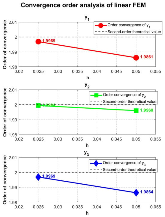
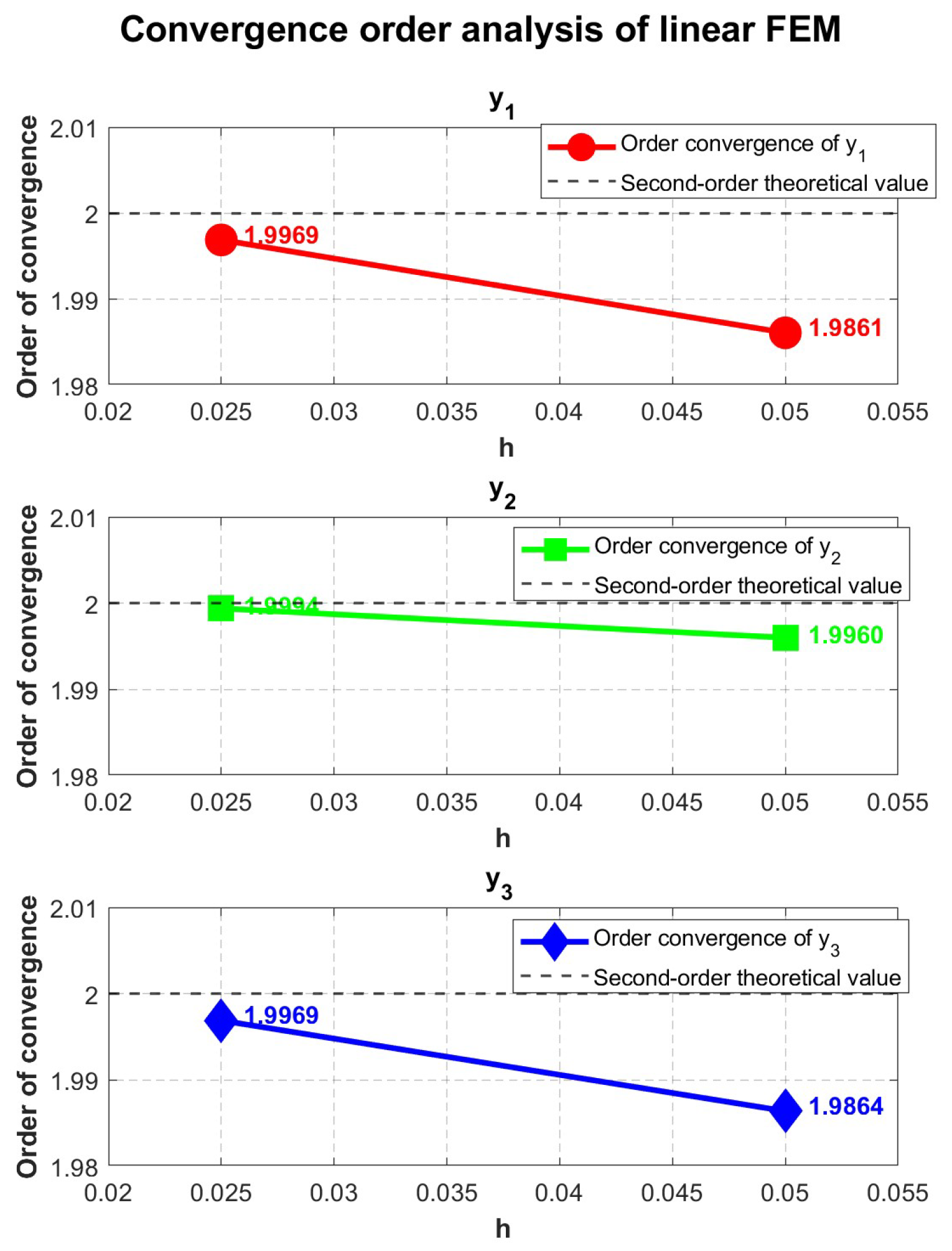
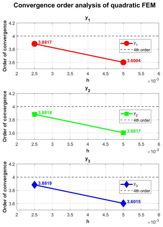
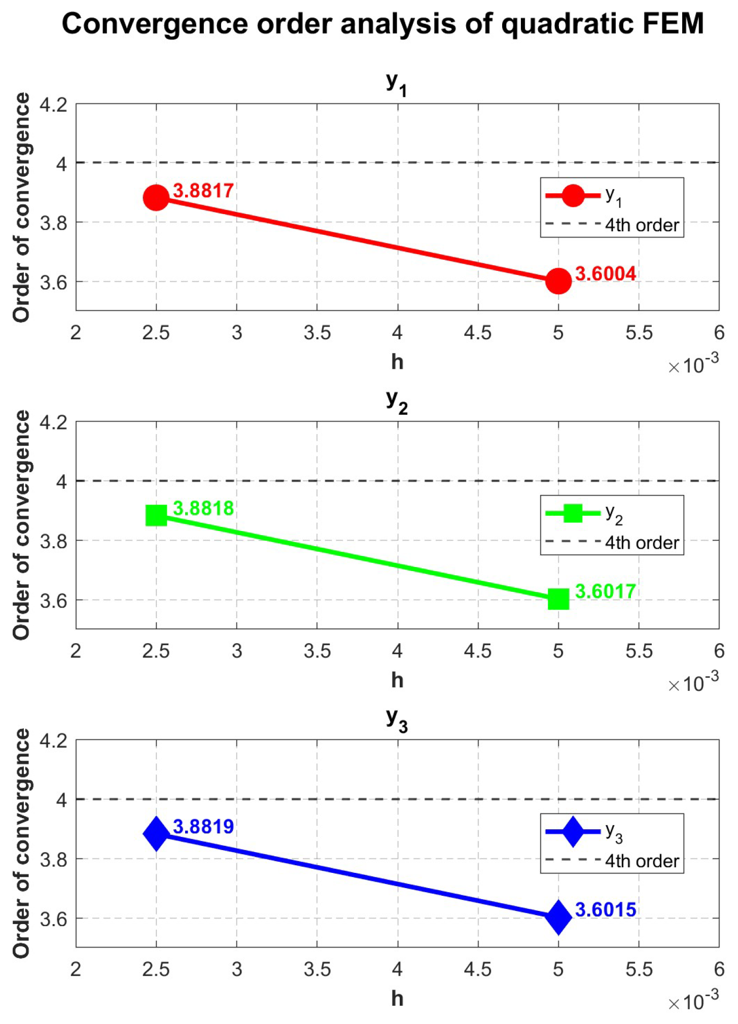
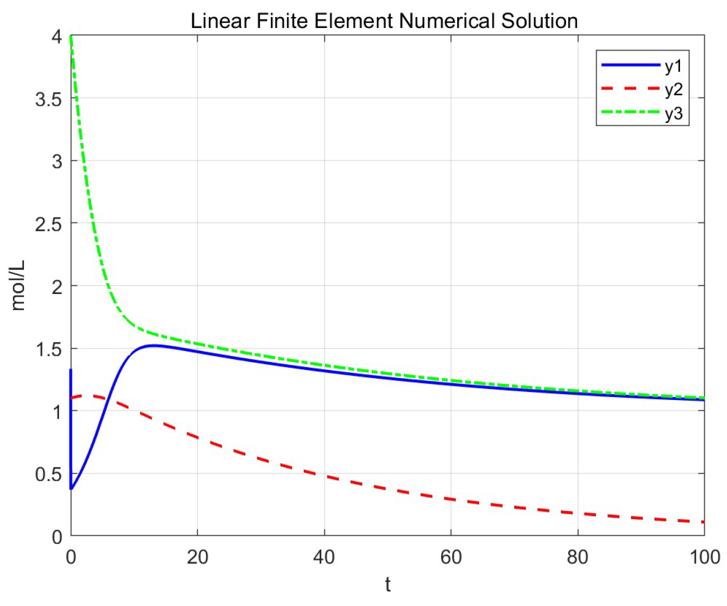
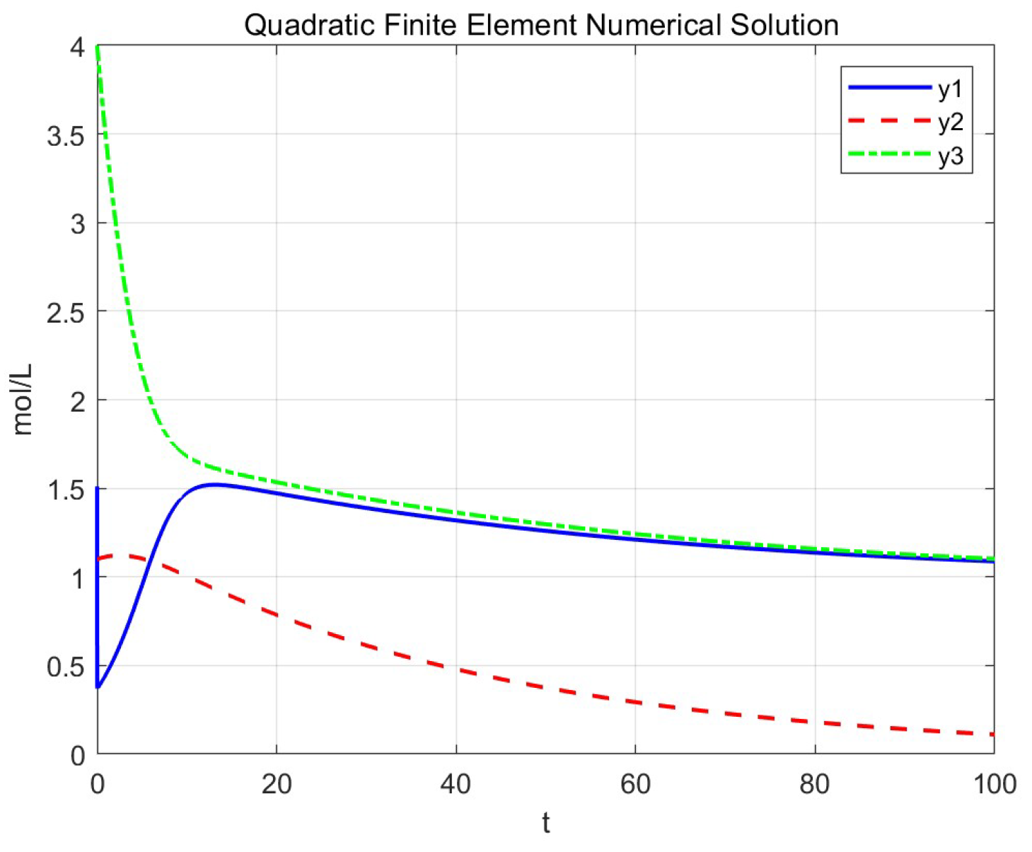
From Figure 1 and Figure 2, order of convergence of linear FEM and quadratic FEM are approximately 2 and 4, respectively. From Figure 3 and Figure 4, the image change trends of linear FEM and quadratic FEM are consistent, when $h=0.005,T=100$.

Figure 1. The order of convergence of linear FEM.

Figure 2. The order of convergence of quadratic FEM.

Figure 3. Image of the linear FEM at $h=0.005$.

Figure 4. Image of the quadratic FEM at $h=0.005$.

From Table 1, when $h=0.001,T=100$ the maximum absolute error of the linear FEM reaches ${10}^{-9}$, while that of BDF2 is only ${10}^{-6}$. This shows that the linear FEM has more advantages. From Table 2, the convergence orders of both the linear FEM and BDF2 are approximately two. From Table 3, linear FEM and BDF2 are both computationally efficient, the FEM exhibiting slightly lower runtime. From Table 4 and Table 5, both linear FEM and ROS2 maintain the theoretical second-order convergence and achieve relatively high computational accuracy, reaching ${10}^{-6}$ when $h=0.1$.

Table 1. Maximum absolute errors between the linear FEM and BDF2.

h	$\parallel {\mathit{y}}_{1\mathit{h}}-{\mathit{y}}_{1\mathit{h}/2}{\parallel }_{\mathit{\infty }}$		$\parallel {\mathit{y}}_{2\mathit{h}}-{\mathit{y}}_{2\mathit{h}/2}{\parallel }_{\mathit{\infty }}$		$\parallel {\mathit{y}}_{3\mathit{h}}-{\mathit{y}}_{3\mathit{h}/2}{\parallel }_{\mathit{\infty }}$
	Linear FEM	BDF2	Linear FEM	BDF2	Linear FEM	BDF2
0.001	4.3046 × ${10}^{-9}$	1.4454 × ${10}^{-2}$	3.5195 × ${10}^{-10}$	3.2285 × ${10}^{-6}$	4.3833 × ${10}^{-9}$	1.0041 × ${10}^{-5}$
0.0005	1.0761 × ${10}^{-9}$	4.0450 × ${10}^{-3}$	8.8003 × ${10}^{-11}$	9.0351 × ${10}^{-7}$	1.0958 × ${10}^{-9}$	2.8104 × ${10}^{-6}$
0.00025	2.6902 × ${10}^{-10}$	1.0669 × ${10}^{-3}$	2.1997 × ${10}^{-11}$	2.3832 × ${10}^{-7}$	2.7396 × ${10}^{-10}$	7.4142 × ${10}^{-7}$

Table 2. Convergence orders between the linear FEM and BDF2.

h	Order of ${\mathit{y}}_1$		Order of ${\mathit{y}}_2$		Order of ${\mathit{y}}_3$
	Linear FEM	BDF2	Linear FEM	BDF2	Linear FEM	BDF2
0.0005	1.9933	1.8373	2.0000	1.8373	1.9934	1.8371
0.00025	2.0054	1.9227	2.0000	1.9226	2.0053	1.9224

Table 3. CPU(s) for the linear FEM and BDF2.

h	CPU of Linear FEM	CPU of BDF2
0.001	0.2688	0.6090
0.0005	0.5341	1.0899
0.00025	1.0330	1.7760

Table 4. Maximum absolute errors between the linear FEM and ROS2.

h	$\parallel {\mathit{y}}_{1\mathit{h}}-{\mathit{y}}_{1\mathit{h}/2}{\parallel }_{\mathit{\infty }}$		$\parallel {\mathit{y}}_{2\mathit{h}}-{\mathit{y}}_{2\mathit{h}/2}{\parallel }_{\mathit{\infty }}$		$\parallel {\mathit{y}}_{3\mathit{h}}-{\mathit{y}}_{3\mathit{h}/2}{\parallel }_{\mathit{\infty }}$
	Linear FEM	ROS2	Linear FEM	ROS2	Linear FEM	ROS2
0.1	3.7120 × ${10}^{-5}$	8.0430 × ${10}^{-5}$	1.2458 × ${10}^{-6}$	2.7322 × ${10}^{-6}$	1.7366 × ${10}^{-5}$	3.3079 × ${10}^{-5}$
0.05	9.3697 × ${10}^{-6}$	2.0489 × ${10}^{-5}$	3.1231 × ${10}^{-7}$	7.5711 × ${10}^{-7}$	4.3826 × ${10}^{-6}$	8.5241 × ${10}^{-6}$
0.025	2.3475 × ${10}^{-6}$	5.0618 × ${10}^{-6}$	7.8111 × ${10}^{-8}$	2.0216 × ${10}^{-7}$	1.0980 × ${10}^{-6}$	2.1419 × ${10}^{-6}$

Table 5. Convergence orders between the linear FEM and ROS2.

h	Order of ${\mathit{y}}_1$		Order of ${\mathit{y}}_2$		Order of ${\mathit{y}}_3$
	Linear FEM	ROS2	Linear FEM	ROS2	Linear FEM	ROS2
0.05	1.9861	1.9731	1.9960	1.8507	1.9864	1.9559
0.025	1.9969	2.0170	1.9994	1.9054	1.9969	1.9920

From Table 6, with $h=0.001,T=100$, the maximum absolute error of the quadratic FEM reaches ${10}^{-12}$, while BDF4 can only reach ${10}^{-7}$. This demonstrates a clear accuracy advantage of the quadratic FEM. From Table 7, the convergence orders of both the quadratic FEM and BDF4 are approximately four. From Table 8, the quadratic FEM and BDF4 are computationally efficient, the FEM exhibiting a lower runtime. From Table 9, with $h=0.01,T=100$, the maximum absolute error of the quadratic FEM reaches ${10}^{-9}$, while IRK4 can only reach ${10}^{-6}$. This demonstrates a distinct accuracy advantage of the quadratic FEM. From Table 10, the convergence order of both the quadratic FEM and IRK4 consistently approaches four.

Table 6. Maximum absolute errors between the quadratic FEM and BDF4.

h	$\parallel {\mathit{y}}_{1\mathit{h}}-{\mathit{y}}_{1\mathit{h}/2}{\parallel }_{\mathit{\infty }}$		$\parallel {\mathit{y}}_{2\mathit{h}}-{\mathit{y}}_{2\mathit{h}/2}{\parallel }_{\mathit{\infty }}$		$\parallel {\mathit{y}}_{3\mathit{h}}-{\mathit{y}}_{3\mathit{h}/2}{\parallel }_{\mathit{\infty }}$
	Quadratic FEM	BDF4	Quadratic FEM	BDF4	Quadratic FEM	BDF4
0.002	1.7870 × ${10}^{-11}$	5.3510 × ${10}^{-3}$	5.0999 × ${10}^{-12}$	1.1956 × ${10}^{-6}$	6.1427 × ${10}^{-11}$	3.7222 × ${10}^{-6}$
0.001	1.1243 × ${10}^{-12}$	4.7908 × ${10}^{-4}$	3.2307 × ${10}^{-13}$	1.0713 × ${10}^{-7}$	3.8956 × ${10}^{-12}$	3.3432 × ${10}^{-7}$
0.0005	8.4155 × ${10}^{-14}$	3.6263 × ${10}^{-5}$	2.3759 × ${10}^{-14}$	8.1140 × ${10}^{-9}$	2.4070 × ${10}^{-13}$	2.5362 × ${10}^{-8}$

Table 7. Convergence orders between the quadratic FEM and BDF4.

h	Order of ${\mathit{y}}_1$		Order of ${\mathit{y}}_2$		Order of ${\mathit{y}}_3$
	Quadratic FEM	BDF4	Quadratic FEM	BDF4	Quadratic FEM	BDF4
0.001	3.9904	3.4815	3.9806	3.4803	3.9790	3.4769
0.0005	3.7398	3.7237	3.8789	3.7229	4.0165	3.7205

Table 8. CPU(s) for the quadratic FEM and BDF4.

h	CPU of Quadratic FEM	CPU of BDF4
0.002	0.2637	0.3335
0.001	0.5223	0.6245
0.0005	1.0037	1.1715
0.00025	1.9047	2.0081

Table 9. Maximum absolute errors between the quadratic FEM and IRK4.

h	$\parallel {\mathit{y}}_{1\mathit{h}}-{\mathit{y}}_{1\mathit{h}/2}{\parallel }_{\mathit{\infty }}$		$\parallel {\mathit{y}}_{2\mathit{h}}-{\mathit{y}}_{2\mathit{h}/2}{\parallel }_{\mathit{\infty }}$		$\parallel {\mathit{y}}_{3\mathit{h}}-{\mathit{y}}_{3\mathit{h}/2}{\parallel }_{\mathit{\infty }}$
	Quadratic FEM	IRK4	Quadratic FEM	IRK4	Quadratic FEM	IRK4
0.01	7.7193 × ${10}^{-9}$	4.2379 × ${10}^{-2}$	1.8607 × ${10}^{-9}$	9.4718 × ${10}^{-6}$	2.2798 × ${10}^{-8}$	2.9519 × ${10}^{-5}$
0.005	6.3642 × ${10}^{-10}$	3.3649 × ${10}^{-3}$	1.5327 × ${10}^{-10}$	7.5192 × ${10}^{-7}$	1.8782 × ${10}^{-9}$	2.3420 × ${10}^{-6}$
0.0025	4.3174 × ${10}^{-11}$	1.9792 × ${10}^{-4}$	1.0397 × ${10}^{-11}$	4.4227 × ${10}^{-8}$	1.2740 × ${10}^{-10}$	1.3775 × ${10}^{-7}$

Table 10. Convergence orders between the quadratic FEM and IRK4.

h	Order of ${\mathit{y}}_1$		Order of ${\mathit{y}}_2$		Order of ${\mathit{y}}_3$
	Quadratic FEM	IRK4	Quadratic FEM	IRK4	Quadratic FEM	IRK4
0.005	3.6004	3.6547	3.6017	3.6550	3.6015	3.6558
0.0025	3.8817	4.0876	3.8818	4.0876	3.8819	4.0876

4.2. Numerical Experiments of Non-Autonomous Stiff ODEs

Defining maximum overall error as $Erro{r}_{y_1}+Erro{r}_{y_2}$

Consider the IVP of a nonlinear autonomous stiff system

$$\left\{\begin{array}{cc}\hfill y_1^{\prime }\left(t\right)=& -100y_1^{10}\left(t\right)+y_2^2\left(t\right)+100{(2+sint)}^{10}-{cos}^{2}t+5cost-4\hfill \\ \hfill y_2^{\prime }\left(t\right)=& y_1\left(t\right)-1000y_2^2\left(t\right)+1000{(2-cost)}^2-2\hfill \\ \hfill y_1\left(0\right)=& 2,y_2\left(0\right)=1\hfill \end{array}\right.$$

(95)

$0\le t\le 100$. This problem possesses a unique exact solution

$$\left\{\begin{array}{cc}\hfill y_1\left(t\right)& =2+sint,\hfill \\ \hfill y_2\left(t\right)& =2-cost\hfill \end{array}\right.$$

(96)

At $t=0$, substituting the initial values yields a stiffness ratio of $256\gg 1$, suggesting that the set of ordinary differential equations exhibits strong stiffness at the initial time.

The numerical solution steps of the linear finite element method and the quadratic finite element method are the same as those in (88), except that the five-point Gaussian quadrature formula is used here.

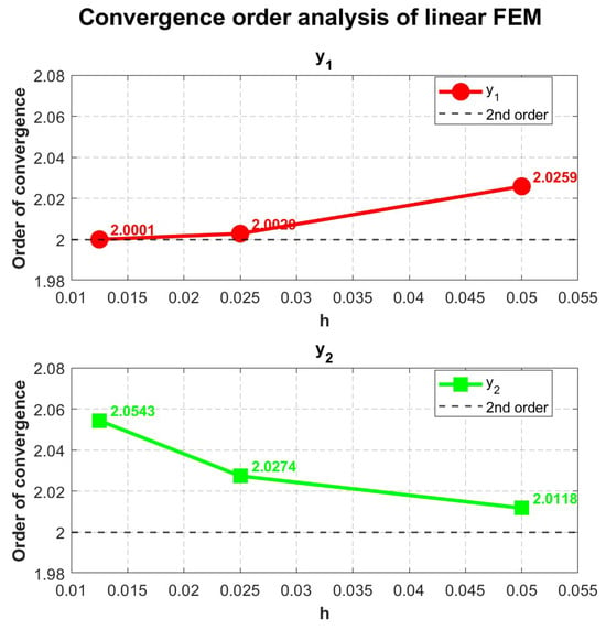
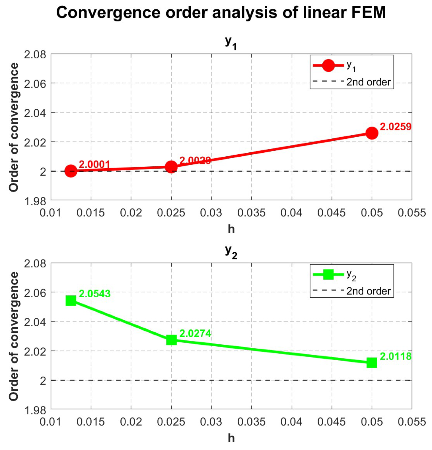
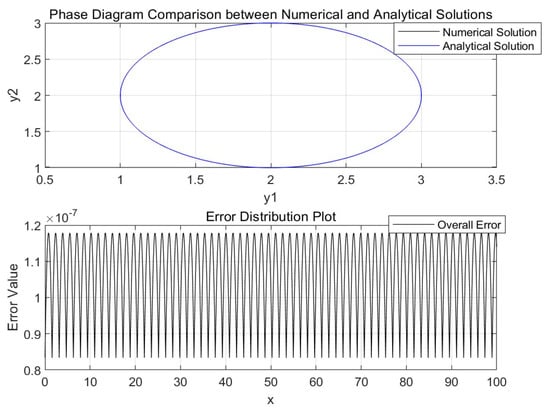
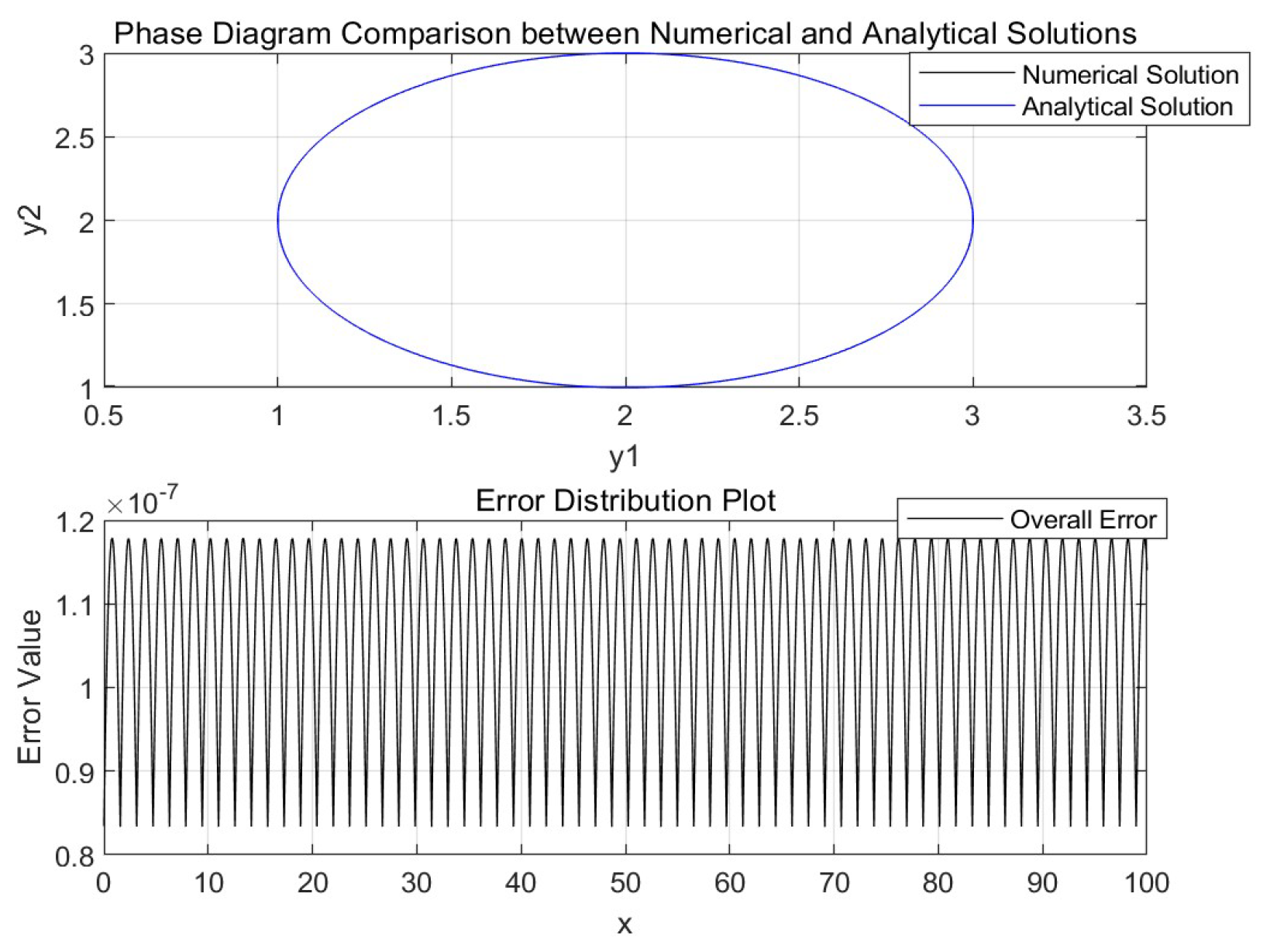
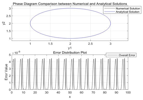
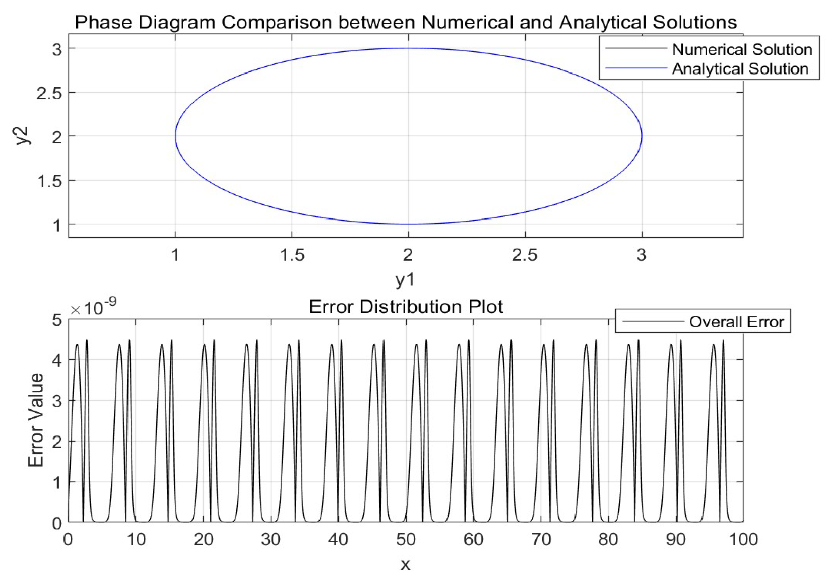
From Figure 5, order of convergence of linear FEM is approximately 2. From Figure 6 and Figure 7, when $h=0.005,T=100$, the phase diagrams of linear FEM and quadratic FEM are highly consistent with the exact solution’s phase diagram, and the errors can reach $1.2\times {10}^{-7}$ and $5\times {10}^{-9}$ respectively.

Figure 5. The order of convergence of linear FEM.

Figure 6. Phase portrait comparison and error plot of the linear FEM at $h=0.005$.

Figure 7. Phase portrait comparison and error plot of the quadratic FEM at $h=0.005$.

From Table 11, with $h=0.001,T=100$, both the linear FEM and BDF2 achieve relatively high computational accuracy with ${10}^{-7}$. In terms of CPU performance, the linear FEM exhibits an advantage over BDF2. From Table 12, the convergence orders of the linear FEM and BDF2 are both approximately two. From Table 13 and Table 14, with $h=0.1,T=100$ the accuracy of $y_1$ can reach ${10}^{-4}$ by the linear FEM, while ROS2 only reaches ${10}^{-2}$. The linear FEM can maintain a convergence order of two, while the ROS2 method only reaches a first-order convergence.

Table 11. Maximum overall error and CPU of the linear FEM and BDF2.

h	Maximum Global Error		CPU Time (s)
	Linear FEM	BDF2	Linear FEM	BDF2
0.001	1.6667 × ${10}^{-7}$	1.6673 × ${10}^{-7}$	1.4090	3.2424
0.0005	4.1667 × ${10}^{-8}$	6.2517 × ${10}^{-8}$	2.4803	6.7853
0.00025	1.0417 × ${10}^{-8}$	2.0838 × ${10}^{-8}$	4.6230	64.2049
0.000125	2.6042 × ${10}^{-9}$	7.1440 × ${10}^{-9}$	7.4952	105.7605

Table 12. Convergence orders between the linear FEM and BDF2.

h	Order of ${\mathit{y}}_1$		Order of ${\mathit{y}}_2$
	Linear FEM	BDF2	Linear FEM	BDF2
0.0005	2.0000	2.0013	2.0000	1.4152
0.00025	2.0000	1.9999	2.0000	1.5851
0.000125	2.0000	1.9965	2.0000	1.5444

Table 13. Maximum absolute error and CPU of the linear FEM and ROS2.

h	Error of ${\mathit{y}}_1$		Error of ${\mathit{y}}_2$
	Linear FEM	ROS2	Linear FEM	ROS2
0.1	8.5019 × ${10}^{-4}$	4.8814 × ${10}^{-2}$	1.6465 × ${10}^{-3}$	3.4806 × ${10}^{-2}$
0.05	2.0877 × ${10}^{-4}$	2.1995 × ${10}^{-2}$	4.0827 × ${10}^{-4}$	1.6949 × ${10}^{-2}$
0.025	5.2087 × ${10}^{-5}$	1.1783 × ${10}^{-2}$	1.0015 × ${10}^{-4}$	8.3205 × ${10}^{-3}$
0.0125	1.3021 × ${10}^{-5}$	6.0819 × ${10}^{-3}$	2.4112 × ${10}^{-5}$	4.0814 × ${10}^{-3}$

Table 14. Convergence orders between the linear FEM and ROS2.

h	Order of ${\mathit{y}}_1$		Order of ${\mathit{y}}_2$
	Linear FEM	ROS2	Linear FEM	ROS2
0.05	2.0259	1.1501	2.0118	1.0381
0.025	2.0029	0.9005	2.0274	1.0265
0.0125	2.0001	0.9541	2.0543	1.0276

From Table 15, with $h=0.0025,T=100$, both the quadratic FEM and IRK4 attain relatively high computational accuracy, the quadratic FEM reaching ${10}^{-8}$ and IRK4 reaching ${10}^{-7}$. The convergence orders of both methods maintain an order of four.

Table 15. Maximum global error and order of convergence for $y_2$ using quadratic FEM and IRK4.

h	Maximum Global Error		Order of ${\mathit{y}}_2$
	Quadratic FEM	IRK4	Quadratic FEM	IRK4
0.01	1.1836 × ${10}^{-6}$	4.0355 × ${10}^{-6}$	*	*
0.005	2.3903 × ${10}^{-4}$	8.1244 × ${10}^{-7}$	4.0051	3.9985
0.0025	4.9369 × ${10}^{-8}$	1.4358 × ${10}^{-7}$	4.0016	3.9999
0.00125	8.3160 × ${10}^{-9}$	2.0015 × ${10}^{-8}$	4.0002	3.9998

* indicates that the step size is the initial step size.

5. Conclusions

(1).

This paper proposes to solve stiff ordinary differential equations by using COFEM, which has a relatively weaker regularity requirement for the solution of the function.

(2).

In the stability analysis, it is proved that the linear FEM and the quadratic FEM have A-stability and unconventional stability in the autonomous ordinary differential equation problem, and have exponential dichotomy in the non-autonomous ordinary differential equation problem.

(3).

In the numerical experiments on nonlinear autonomous and non-autonomous stiff ODEs (including strongly and moderately stiff cases), a relatively large step size of $h=0.1$ was adopted over a longer period of time, with the numerical solution accuracy reaching ${10}^{-4}$. The superconvergence order consistent with the theory was maintained, providing a good approach for the numerical calculation of stiff differential equations.

Future research will investigate adaptive strategies, nonlinear stability limits for strongly stiff systems, and the performance of the proposed method for problems with extreme stiffness ratios.

References

- Arrhenius, S. On the Reaction Velocity of the Inversion of Cane Sugar by Acids. Chem. Kinet. 1967, 4, 31–35. [Google Scholar]
- Field, R.J.; Noyes, R.M. Oscillations in chemical systems. V. Quantitative explanation of band migration in the Belousov-Zhabotinskii reaction. J. Am. Chem. Soc. 2002, 96, 2001–2006. [Google Scholar] [CrossRef] [Scilit]
- Bui, T.D. Solving stiff differential equations in the simulation of physical systems. Simulation 1981, 37, 37–46. [Google Scholar] [CrossRef] [Scilit]
- Aliyu, B.K.; Osheku, C.A.; Funmilayo, A.A.; Musa, J.I. Identifying stiff ordinary differential equations and problem solving environments (PSEs). J. Sci. Res. Rep. 2014, 3, 1430–1448. [Google Scholar] [CrossRef] [Scilit]
- Frank, R.; Schneid, J.; Ueberhuber, C.W. Order results for implicit Runge–Kutta methods applied to stiff systems. SIAM J. Numer. Anal. 1985, 22, 515–534. [Google Scholar] [CrossRef] [Scilit]
- Abd Rasid, N.; Ibrahim, Z.B.; Majid, Z.A.; Ismail, F. Formulation of a new implicit method for group implicit BBDF in solving related stiff ordinary differential equations. Statistics 2021, 9, 144–150. [Google Scholar] [CrossRef] [Scilit]
- Junaidi, S.A.; Jaafar, B.A.; Zawawi, I.S.M. Composite backward differentiation formulas for solving stiff ordinary differential equation. AIP Conf. Proc. 2024, 3189, 070005. [Google Scholar] [CrossRef] [Scilit]
- Shampine, L.F.; Sommeijer, B.P.; Verwer, J.G. IRKC: An IMEX solver for stiff diffusion–reaction PDEs. J. Comput. Appl. Math. 2006, 196, 485–497. [Google Scholar] [CrossRef] [Scilit]
- Cardone, A.; D’Ambrosio, R.; Paternoster, B. Exponentially fitted IMEX methods for advection–diffusion problems. J. Comput. Appl. Math. 2017, 316, 100–108. [Google Scholar] [CrossRef] [Scilit]
- Xiao, A.; Zhang, G.; Yi, X. Two classes of implicit–explicit multistep methods for nonlinear stiff initial-value problems. Appl. Math. Comput. 2014, 247, 47–60. [Google Scholar] [CrossRef] [Scilit]
- Selvakumar, K.; Jason, K. L-stable and A-stable numerical method of order two for stiff differential equation. Soft Comput. 2022, 26, 12779–12794. [Google Scholar] [CrossRef] [Scilit]
- Rufai, M.A.; Tran, T.; Anastassi, Z.A. A variable step-size implementation of the hybrid Nyström method for integrating Hamiltonian and stiff differential systems. Comput. Appl. Math. 2023, 42, 156. [Google Scholar] [CrossRef] [Scilit]
- Ramos, H.; Rufai, M.A. A new one-step method with three intermediate points in a variable step-size mode for stiff differential systems. J. Math. Chem. 2023, 61, 673–688. [Google Scholar] [CrossRef] [Scilit]
- Calvo, M.; Montijano, J.I.; Rández, L. Modified Singly-Runge–Kutta-TASE Methods for the Numerical Solution of Stiff Differential Equations. J. Sci. Comput. 2025, 103, 3. [Google Scholar] [CrossRef] [Scilit]
- Calvo, M.; Fu, L.; Montijano, J.I.; Rández, L. Singly TASE operators for the numerical solution of stiff differential equations by explicit Runge–Kutta schemes. J. Sci. Comput. 2023, 96, 17. [Google Scholar] [CrossRef] [Scilit]
- Hindenlang, F.; Gassner, G.J.; Altmann, C.; Beck, A.; Staudenmaier, M. Explicit discontinuous Galerkin methods for unsteady problems. Comput. Fluids 2012, 61, 86–93. [Google Scholar] [CrossRef] [Scilit]
- Ten Eyck, A.; Lew, A. Discontinuous Galerkin methods for non-linear elasticity. Int. J. Numer. Methods Eng. 2006, 67, 1204–1243. [Google Scholar] [CrossRef] [Scilit]
- Xia, Y.; Xu, Y.; Shu, C. Efficient time discretization for local discontinuous Galerkin methods. Discrete Contin. Dyn. Syst. Ser. B 2007, 8, 677. [Google Scholar] [CrossRef] [Scilit]
- Al-Aradi, A.; Correia, A.; Jardim, G.; Freitas Naif, D. Extensions of the deep Galerkin method. Appl. Math. Comput. 2022, 430, 127287. [Google Scholar] [CrossRef] [Scilit]
- Hulbert, G.M. Time finite element methods for structural dynamics. Int. J. Numer. Methods Eng. 1992, 333, 307–331. [Google Scholar] [CrossRef] [Scilit]
- Tang, Q.; Chen, C.; Liu, L. Energy conservation and symplectic properties of continuous finite element methods for Hamiltonian systems. Appl. Math. Comput. 2006, 181, 1357–1368. [Google Scholar] [CrossRef] [Scilit]
- Tang, Q.; Chen, C.; Liu, L. Space-time finite element method for Schrödinger equation and its conservation. Appl. Math. Mech. 2006, 27, 335–340. [Google Scholar] [CrossRef] [Scilit]
- Tang, Q.; Chen, C. Continuous finite element methods for Hamiltonian systems. Appl. Math. Mech. 2007, 27, 1071–1080. [Google Scholar] [CrossRef] [Scilit]
- Yang, Y.L.; Tang, Q. Superconvergence of continuous finite elements for initial value problems of ordinary differential equations. Numer. Math. J. Chin. Univ. 2004, 26, 91–96. [Google Scholar]
- Cui, Q.Q. A Solution Method for Stiff Ordinary Differential Equations. Master’s Thesis, Beijing University of Technology, Beijing, China, 2019. [Google Scholar] [CrossRef]
- Zhang, Y.L.; Wang, M.S.; Hong, L. Research on Solving Rigid Problems in Systems Biology Using Neural Networks. Acta Sci. Nat. Univ. Sunyatseni 2024, 63, 265–274. [Google Scholar]
Disclaimer/Publisher’s Note: The statements, opinions and data contained in all publications are solely those of the individual author(s) and contributor(s) and not of MDPI and/or the editor(s). MDPI and/or the editor(s) disclaim responsibility for any injury to people or property resulting from any ideas, methods, instructions or products referred to in the content. |
© 2026 by the authors. Licensee MDPI, Basel, Switzerland. This article is an open access article distributed under the terms and conditions of the Creative Commons Attribution (CC BY) license.