Modeling COVID-19 Population Dynamics with a Viral Reservoir and Human Mobility

Abstract

This article introduces and thoroughly examines a novel deterministic compartmental model of COVID-19 dynamics. The model uniquely incorporates compartments for symptomatic and asymptomatic individuals alongside an environmental reservoir for the pathogen. It also accounts for a steady inflow of infected visitors and a steady outflow from the removed class. The mathematical soundness of the model is established by identifying the invariant region and ensuring positivity of solutions. Notably, during surges of infected visitors, certain classes maintain positive minimum values. We analytically determine endemic equilibrium points and prove the global stability of the disease-free equilibrium. Sensitivity analysis highlights the significant roles of transmission rates and asymptomatic individuals in disease spread. Simulation results corroborate the theoretical findings and provide additional insights into the model’s predictive capabilities.

1. Introduction

COVID-19, resulting from the SARS-CoV-2 virus, surfaced as a worldwide pandemic in late 2019 and rapidly disseminated globally, significantly affecting public health infrastructures and changing how societies operated. SARS-CoV-2 is part of the coronavirus family, yet it differs in many aspects compared to SARS-CoV (2002–2003) and MERS-CoV (2012). For example, Zhang et al. provided a comparative genomic analysis showing notable structural differences [1], while Zhou et al. identified the novel virus’s probable bat origin and unique spike protein characteristics [2]. What distinguished SARS-CoV-2 was its unmatched transmission speed and the wide spectrum of clinical manifestations observed in affected individuals. Guan et al. reported that patients exhibited symptoms ranging from mild respiratory distress to severe pneumonia and organ failure [3]. Authors Huang et al. highlighted the rapid progression of disease severity in hospitalized patients during the early outbreak in Wuhan [4]. Wiersinga et al. provided a comprehensive overview of COVID-19’s systemic pathophysiology and its unprecedented global impact [5]. At the beginning of the pandemic, experts cautioned that COVID-19 would put pressure on healthcare systems, disturb everyday life, and test government response plans. This underscored the significance of risk management, focusing on preventive strategies and tackling the economic effects, particularly on public finances and healthcare systems. Numerous studies analyzed the challenges in handling the pandemic, highlighting that government measures, like lockdowns, intensified stress on healthcare systems and interrupted vital services. In South Africa, disruptions in healthcare were supported by reports indicating a decrease in emergency room visits, hospital admissions, and primary healthcare services. Nematswerani et al. provided detailed data showing declines in service utilization at major health facilities [6]. South Africa’s pandemic response was examined by De Kadt et al., emphasizing the trade-offs between early lockdown success and the socioeconomic costs [7]. Perez-Talebi et al. explored the macroeconomic risks of pandemic containment, focusing on how emergency interventions affected national fiscal stability [8]. And in their work, McAleer et al. discussed broader global economic disruptions and its cascading effect on national healthcare resilience [9].

As hospitals and public health organizations encountered significant strain, a worldwide scientific initiative was initiated to comprehend the virus and create measures to curb its transmission. Scientists, drug manufacturers, and medical institutions focused on discovering successful therapies and developing vaccines, with the goal of reducing the health and financial impacts of the pandemic. McAleer et al. emphasized the global coordination of research and the urgency of vaccine development [9]. Perez-Talebi et al. underscored the dual focus on healthcare innovation and economic sustainability [8]. Nematswerani et al. highlighted the role of public–private collaboration in accelerating COVID-19 treatment protocols [6], while De Kadt et al. noted how government partnerships with research institutions shaped South Africa’s health policy response [7].

The advancement of vaccines has been a central focus of medical research throughout the COVID-19 pandemic, driving global efforts to produce safe and effective immunizations. By the end of 2020, several vaccines received emergency use authorization, marking a critical milestone. Ahmed, Quadeer, and McKay identified potential vaccine targets through an immunoinformatics approach [10]. McLean et al. analyzed the global impact and uptake of COVID-19 vaccines, highlighting disparities and rollout challenges [11]. And Zhao evaluated long-term immune responses to mRNA vaccines, demonstrating their sustained role in reducing transmission [12]. Collectively, these developments contributed significantly to controlling the spread of the virus and managing the pandemic.

However, the emergence of SARS-CoV-2 variants raised concerns about vaccine effectiveness. Vellingiri et al. reviewed how viral mutations may compromise vaccine efficacy [13]. Chi et al. investigated the immune evasion capabilities of major variants [14], and Luo et al. reported on vaccine performance against emerging strains in real-world settings [15].

In parallel, the exploration of antiviral therapies, particularly through drug repurposing, has yielded mixed outcomes. Slomski assessed metformin, ivermectin, and fluvoxamine in overweight and obese adults, concluding these drugs were ineffective in preventing severe illness [16]. The broader trends in antiviral repurposing were discussed in Martínez’ work, outlining both progress and ongoing limitations in Drug Discovery Today [17]. Additionally, Ford et al., and Shah, Modi, and Sagar compared lopinavir-ritonavir with darunavir-ritonavir in hospitalized patients, finding that lopinavir-ritonavir was associated with improved survival rates [18,19].

Although vaccines have greatly influenced the management of COVID-19, the necessity for continued investigation into effective treatments is essential, particularly given the swiftly changing variants of concern (VOCs). At first, there was optimism that widespread vaccination would result in herd immunity; however, the arrival of variants such as Delta and Omicron, which are more contagious and might partially escape immunity, has reduced this hopeful outlook [4,20]. Recent research has underscored the changing efficacy of COVID-19 vaccines in relation to new variants. Research published in the New England Journal of Medicine revealed that vaccine effectiveness (VE) against the Omicron variant was considerably diminished in comparison to the Delta variant, with immunity declining over time, particularly after the initial two doses [21]. A systematic review and meta-analysis published in BMC Medicine indicated that complete vaccination offered differing levels of protection against various variants, showing a vaccine efficacy (VE) of 55.9% against Omicron. Booster shots markedly enhanced vaccine effectiveness against Omicron to 80.8% [22]. These variants highlight the virus’s changing traits and its ability to evolve, resulting in doubts about lasting immunity and the chance of reinfection. A research article in The Lancet Microbe investigated the longevity of immunity to reinfection by SARS-CoV-2, showing significant variation in antibody reduction and reinfection chances over time, highlighting the need for ongoing tracking of immune responses and adjusting vaccination approaches [23]. In a similar vein, a recent systematic review and meta-analysis conducted by Stein et al. emphasized that although protection against severe illness stays strong for a minimum of 10 months after infection, immunity against reinfection, especially with the Omicron variant, decreases at a faster rate [24]. Therefore, while vaccines and antiviral treatments are essential tools in fighting COVID-19, additional research is necessary to address these challenges. An extensive study performed by prominent microbiologists at the Icahn School of Medicine at Mount Sinai shows that the antibody responses generated by COVID-19 vaccines endure over time. The research, appearing online in Immunity on 22 February 2024, disputes the notion that immunity from mRNA vaccines diminishes rapidly and shows that those with existing immunity had quicker and stronger antibody responses, highlighting the necessity to update vaccination strategies for new variants [25]. Furthermore, Australian scientists are developing mRNA vaccines aimed at immune evasion by variants such as Omicron, demonstrating encouraging rises in antibody responses. Studies have demonstrated that immunity from both infections and vaccines can produce enduring antibody responses; however, an initial decline is succeeded by a stabilization period, emphasizing the need for ongoing vaccine development and oversight [26]. In addition, existing immunity greatly influences reactions to mRNA boosters, indicating that booster approaches ought to be customized according to a person’s immune background for maximum effectiveness [27].

In the realm of mathematical modeling, various studies have explored the dynamics of COVID-19 transmission, including the incorporation of environmental reservoirs. For example, in their paper [28], Mwalili et al. proposed a modified SEIR model that considers pathogen reservoirs in the environment, with a focus on social distancing and other interventions to curb the epidemic. While their model effectively captures the role of environmental reservoirs, it lacks the detailed mathematical analysis and stability results that our study provides. In this article, we extend the work of [28] by developing a more comprehensive deterministic compartmental model that rigorously analyzes the stability of the disease-free and endemic equilibrium points, adding a deeper mathematical understanding of the disease dynamics.

The objective of this paper is to introduce and rigorously analyze a deterministic compartmental model of COVID-19 dynamics. The model features compartments for symptomatic and asymptomatic individuals, incorporates an environmental reservoir for the pathogen, and includes a steady inflow of infected individuals (visitors) and outflow from the removed class. Numerical simulations are also provided to demonstrate the model’s dynamics under various epidemiological scenarios.

Recent developments in the modeling of COVID-19 dynamics have increasingly incorporated environmental reservoirs and additional transmission pathways. For instance, Akingbade and Ayegbusi formulated a deterministic compartmental model featuring pathogen reservoirs and conducted thorough equilibrium and stability analyses [29]. Similarly, Khan et al. extended such frameworks to stochastic differential models, examining extinction and persistence conditions under environmental and demographic noise [30]. Moreover, a recent study introduced periodic transmission dynamics alongside environmental compartments, using South African data to fit and analyze model behavior under seasonal effects [31]. These advances underscore the growing sophistication of reservoir-based COVID-19 models, to which our work further contributes by adding visitor inflow and a dual infectious class structure supported by a complete mathematical stability analysis.

Structure of the Paper

In Section 2, we present our mathematical model, which is derived from a system of ordinary differential equations (ODEs) and comprises five compartments that symbolize various phases of infection. Section 3 outlines the parameters and initial conditions for the model that simulates the infectious disease dynamics, encompassing transmission, recovery rates, and population data. In Section 4, we examine the constraints and non-negativity of the model’s solutions, confirming that they stay plausible in the biological setting. Section 5 deals with equilibria of the model system and the basic reproduction number. In Section 6, we explore the presence of the endemic equilibrium, whereas Section 7 discusses the global stability of the disease-free equilibrium, presuming no arrival of infected individuals. In Section 8, we provide simulation outcomes, followed by discussions in Section 9, where we outline the main findings and possible effects on public health policy, and discuss possible future work.

2. Mathematical Model

One of the methods to describe the transmission of diseases among populations is through compartmental models. In these models, individuals are grouped into sections such as S (susceptible), E (exposed), I (infected), and R (removed), each representing a distinct phase of the illness. These models assume a well-mixed population, where any two individuals have the same probability of contracting the infection. Furthermore, to accurately depict the disease progression at time t, assumptions must be made regarding the routes of infection and the transitions between compartments. Given the role of migrant communities and the behavior of SARS-CoV-2 in the COVID-19 context, it is essential that the model captures interactions among these groups.

We propose a mathematical model to describe the transmission dynamics of COVID-19, incorporating symptomatic and asymptomatic infected individuals, an environmental reservoir, and the inflow of migrants. Accordingly, we consider a host or local-migrant population together with migrants who visit this population just for short stays. We refer to such a population as a host–migrant population. The model classifies the host population into four groups: susceptible $S\left(t\right)$, symptomatic infectious $I\left(t\right)$, asymptomatic infectious $A\left(t\right)$, and removed $R\left(t\right)$. Then there is a fifth compartment, the environmental reservoir $P\left(t\right)$. For relevant modeling approaches and assumptions, see McAleer [9], Perez and Talebi [8], Ford et al. [18], Cesari [32], and Vyambwera and Witbooi [33].

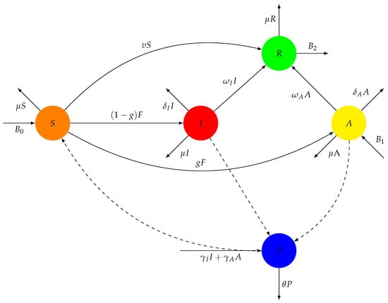
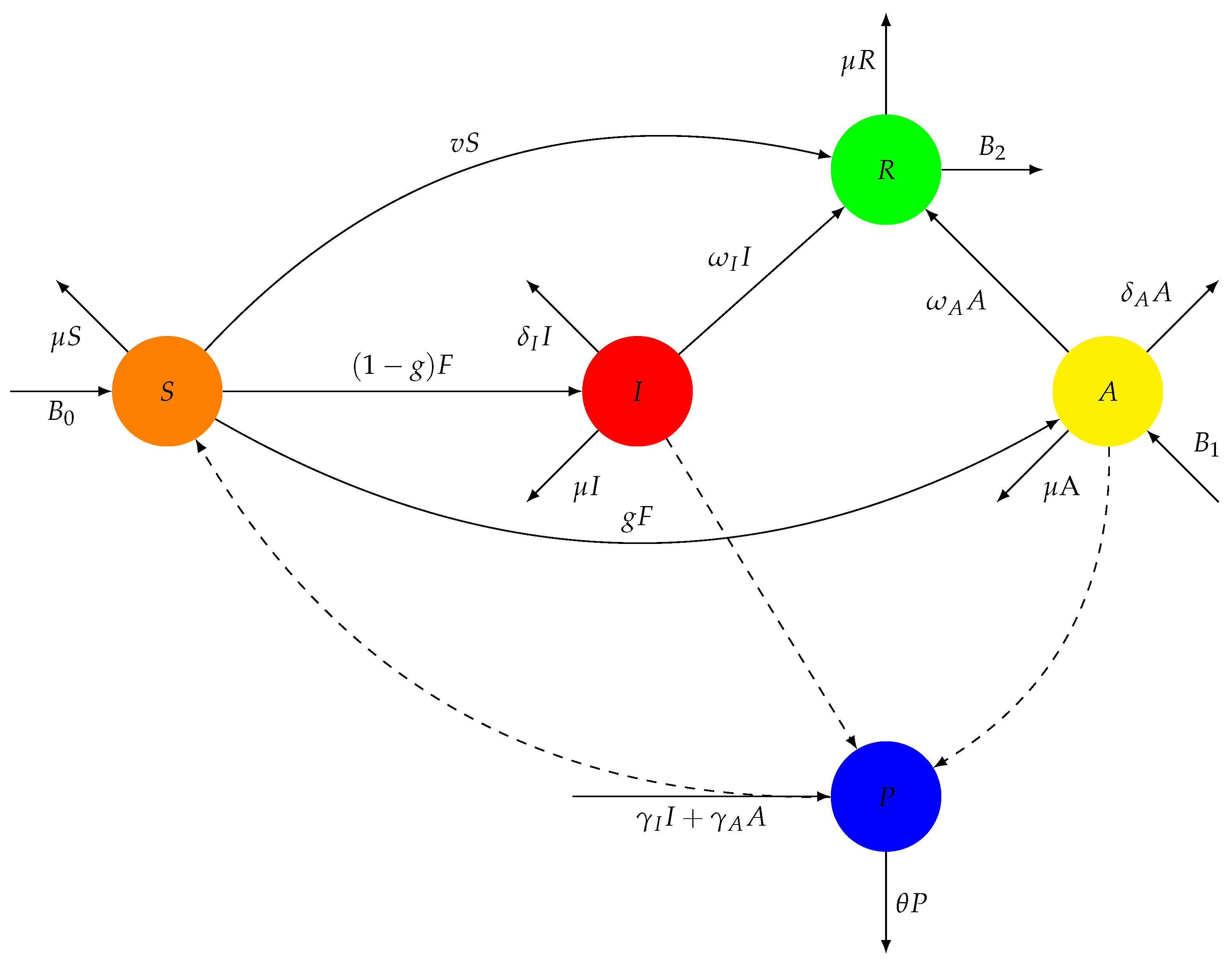
Below in Figure 1 is an illustration of the SIARP model. It shows the human population and the pathogens (COVID-19 virus) in the environmental reservoir, the transition of humans between compartments, and it aims to show the interaction between the humans and the environmental reservoir. The compartmental model is governed by the system (1) of ODE.

Figure 1. The flow chart for the SIARP model.

The compartmental model (1) below illustrates the interplay among the classes S, I, A, R, and P as displayed in Figure 1 above.

$$\begin{array}{c}{\displaystyle \frac{dS}{dt}=B_0-F-{\mu }_{0}S,}\hfill \\ {\displaystyle \frac{dI}{dt}=(1-g)F-{\mu }_{1}I,}\hfill \\ {\displaystyle \frac{dA}{dt}=B_1+gF-{\mu }_{2}A,}\hfill \\ {\displaystyle \frac{dR}{dt}=vS+{\omega }_{I}I+{\omega }_{A}A-\mu R-B_2,}\hfill \\ {\displaystyle \frac{dP}{dt}={\gamma }_{I}I+{\gamma }_{A}A-\theta P,}\hfill \\ {\displaystyle N=S+I+A+R,}\hfill \end{array}$$

(1)

where $F={\displaystyle \frac{\alpha SP}{1+CP}}+\beta S(I+A)$, ${\mu }_0=(\mu +v)$, ${\mu }_1=(\mu +{\delta }_I+{\omega }_I)$, ${\mu }_2=(\mu +{\delta }_A+{\omega }_A)$, and N is the total population.

The deterministic model describes the transmission dynamics of COVID-19 within the South African population using five compartments: susceptible individuals $S\left(t\right)$, symptomatic infected individuals $I\left(t\right)$, asymptomatic infected individuals $A\left(t\right)$, recovered individuals $R\left(t\right)$, and the virus density in the environmental reservoir $P\left(t\right)$. The total population at time t is denoted by $N\left(t\right)=S\left(t\right)+I\left(t\right)+A\left(t\right)+R\left(t\right)$.

The first equation in (1) represents a constant inflow of susceptible individuals at rate $B_0$, modeling natural recruitment (e.g., birth or immigration). Susceptible individuals may become infected via two primary pathways: through contact with the environmental reservoir P, governed by the transmission parameter $\alpha$, or through contact with symptomatic or asymptomatic individuals, governed by the transmission parameter $\beta$. The degree of interaction with the infectious environment is modulated by the factor C. New infections reduce the susceptible population, occurring via the composite force of infection F, which includes both environmental and person-to-person transmission.

Vaccination is represented by the rate v; however, it is set to zero in this model due to the absence of an available vaccine during the study period.

In the second equation, $(1-g)$ represents the proportion of new infections that become symptomatic, while ${\delta }_I$ is the disease-induced mortality rate among symptomatic individuals, and ${\omega }_I$ is their recovery rate.

The third, fourth, and fifth equations in (1) include parameters $B_1$ and $B_2$, which represent the inflow of asymptomatic infected migrants and the outflow of recovered migrants, respectively. Asymptomatic infected individuals (A) also experience disease-induced mortality at rate ${\delta }_A$ and recover at rate ${\omega }_A$.

Both symptomatic and asymptomatic individuals contribute to environmental contamination, at rates ${\gamma }_I$ and ${\gamma }_A$, respectively, increasing the virus density in the reservoir P. The death rate of pathogens in the environment is denoted by $\theta$.

The natural mortality rate $\mu$ applies to all host compartments (S, I, A, R), resulting in loss terms $\mu S$, $\mu I$, $\mu A$, and $\mu R$. Pathogens die at rate $\theta P$.

Over time, the susceptible population declines as individuals become infected, transitioning into the symptomatic or asymptomatic compartments. Infected individuals either recover or die, and recovered individuals may eventually leave the system through migration (as represented by $B_2$). Environmental contamination increases as infected individuals shed the virus, further fueling transmission. This model captures both direct and indirect transmission routes and highlights the dynamics of infection, recovery, mortality, and migration in the context of COVID-19.

3. Model Parameters and Initial Conditions

To explore the dynamics of infectious diseases, we created a mathematical model that includes various essential parameters controlling the transmission, recovery, and advancement of the disease. These factors are essential for modeling how the infection spreads and affects the population as time progresses. The table below displays the main parameters and initial conditions employed in the model simulations. These values were thoughtfully selected based on sensible assumptions regarding population size, disease traits, and epidemiological elements, such as transmission rates, recovery rates, along with birth and death rates. By analyzing these variables, we strive to gain clearer insight into the elements affecting disease transmission and possible interventions.

The model includes various parameters essential for grasping the transmission of infectious diseases. These consist of the overall population count, transmission rates, and the rates for asymptomatic as well as symptomatic infections. Furthermore, the rates of recovery, birth, and death in the population are essential elements that influence the accuracy of the model. The initial conditions are created to represent the population spread across different categories: people susceptible to infection, those showing symptoms and being infectious, individuals asymptomatic yet infectious, people who have recovered from the illness, and those advancing through the phases of the disease.

Clarification on parameter values: The parameter values presented in Table 1 and Table 2 are based on a combination of literature sources, theoretical considerations, and informed estimates relevant to modeling COVID-19 dynamics.

Parameters related to the environmental reservoir, $P\left(t\right)$, are modeled using non-specific units. This approach is common in infectious disease models involving environmental pathways, especially when empirical measurements (such as environmental virus density) are infeasible due to cost and complexity. For example, as in Witbooi et al. [34], abstract units are used to simulate qualitative dynamics effectively.

The chosen parameter values are therefore intended to capture the model’s key behaviors qualitatively, rather than to precisely match a specific dataset. This enables broader applicability of the model structure, including in settings where more detailed or population-specific data are available.

Remark 1. 

Thus we shall regard P as being measured in a unit ${\mathrm{u}}_1$.

Table 1. Parameters with values, descriptions, and units used in the model. Where applicable, time-based rates are expressed per day.

Parameter	Description	Value	Units	Source
$B_0$	Constant inflow rate of susceptibles	$P_0\mu \approx 2500$	person/day	[35]
$B_1$	Influx rate of asymptomatically infected migrants	200	person/day	Nominal
$B_2$	Outflow rate of recovered migrants	${\displaystyle \frac{\left({\omega }_A{B}_1\right)}{(\mu +{\omega }_A+{\delta }_A)}}\approx 199.91$	person/day	Remark 2
$\mu$	Natural (background) death rate	${\displaystyle \frac{1}{65\times 365}}\approx 4.2150\times {10}^{-5}$	1/day	[36]
$P_0$	South African population in 2020	59,308,690	person	[35]
$\alpha$	Transmission rate via environmental reservoir	$0.3\beta \approx 4.0466\times {10}^{-10}$	1/(${\mathrm{u}}_1$·day)	Derived
C	The reciprocal of the half-saturation value of P	0.02	1/${\mathrm{u}}_1$	Estimated
g	Proportion of new infections that are asymptomatic	0.1	Unitless (proportion)	Estimated
$\beta$	Transmission rate via direct contact	${\displaystyle \frac{0.08}{P_0}}\approx 1.3489\times {10}^{-9}$	1/(person·day)	Estimated
v	Rate of vaccination	0	1/day	—
$n,n_1$	Timeline range for simulations	$n=14$, $n_1=7(n+1)$	days	[37]
${\gamma }_I$	Contribution to P from symptomatic individuals	0.05	${\mathrm{u}}_1$/(person·day)	Estimated
${\gamma }_A$	Contribution to P from asymptomatic individuals	0.005	${\mathrm{u}}_1$/(person·day)	Estimated
${\delta }_I$	Death rate due to COVID-19 in infected persons	0.0002	1/day	[38]
${\delta }_A$	Death rate due to COVID-19 in asymptomatic persons	0.0001	1/day	[38]
${\omega }_I$	Recovery rate of symptomatic individuals	0.15	1/day	[38]
${\omega }_A$	Recovery rate of asymptomatic individuals	$2{\omega }_I=0.3$	1/day	[38]
$\theta$	Death rate of pathogens in environmental reservoir	$1/4$	non-specific, ${\mathrm{u}}_1$	Estimated

Table 1. Parameters with values, descriptions, and units used in the model. Where applicable, time-based rates are expressed per day.

Parameter	Description	Value	Units	Source
$B_0$	Constant inflow rate of susceptibles	$P_0\mu \approx 2500$	person/day	[35]
$B_1$	Influx rate of asymptomatically infected migrants	200	person/day	Nominal
$B_2$	Outflow rate of recovered migrants	${\displaystyle \frac{\left({\omega }_A{B}_1\right)}{(\mu +{\omega }_A+{\delta }_A)}}\approx 199.91$	person/day	Remark 2
$\mu$	Natural (background) death rate	${\displaystyle \frac{1}{65\times 365}}\approx 4.2150\times {10}^{-5}$	1/day	[36]
$P_0$	South African population in 2020	59,308,690	person	[35]
$\alpha$	Transmission rate via environmental reservoir	$0.3\beta \approx 4.0466\times {10}^{-10}$	1/(${\mathrm{u}}_1$·day)	Derived
C	The reciprocal of the half-saturation value of P	0.02	1/${\mathrm{u}}_1$	Estimated
g	Proportion of new infections that are asymptomatic	0.1	Unitless (proportion)	Estimated
$\beta$	Transmission rate via direct contact	${\displaystyle \frac{0.08}{P_0}}\approx 1.3489\times {10}^{-9}$	1/(person·day)	Estimated
v	Rate of vaccination	0	1/day	—
$n,n_1$	Timeline range for simulations	$n=14$, $n_1=7(n+1)$	days	[37]
${\gamma }_I$	Contribution to P from symptomatic individuals	0.05	${\mathrm{u}}_1$/(person·day)	Estimated
${\gamma }_A$	Contribution to P from asymptomatic individuals	0.005	${\mathrm{u}}_1$/(person·day)	Estimated
${\delta }_I$	Death rate due to COVID-19 in infected persons	0.0002	1/day	[38]
${\delta }_A$	Death rate due to COVID-19 in asymptomatic persons	0.0001	1/day	[38]
${\omega }_I$	Recovery rate of symptomatic individuals	0.15	1/day	[38]
${\omega }_A$	Recovery rate of asymptomatic individuals	$2{\omega }_I=0.3$	1/day	[38]
$\theta$	Death rate of pathogens in environmental reservoir	$1/4$	non-specific, ${\mathrm{u}}_1$	Estimated

The initial conditions used in the simulations were estimated and are outlined in the following table.

Table 2. Initial conditions with values, descriptions, and units. The value $P_0$ represents the South African population in 2020.

Parameter	Description	Value	Units
$S\left(0\right)$	Susceptible population	$0.995\times P_0$	persons
$I\left(0\right)$	Symptomatic infectious individuals	171,000	persons
$A\left(0\right)$	Asymptomatic infectious individuals	17,000	persons
$R\left(0\right)$	Recovered/removed individuals	0	persons
$P\left(0\right)$	Density of virus in environment	2000	${\mathrm{u}}_1$

Table 2. Initial conditions with values, descriptions, and units. The value $P_0$ represents the South African population in 2020.

Parameter	Description	Value	Units
$S\left(0\right)$	Susceptible population	$0.995\times P_0$	persons
$I\left(0\right)$	Symptomatic infectious individuals	171,000	persons
$A\left(0\right)$	Asymptomatic infectious individuals	17,000	persons
$R\left(0\right)$	Recovered/removed individuals	0	persons
$P\left(0\right)$	Density of virus in environment	2000	${\mathrm{u}}_1$

4. Boundedness and Positivity of Solutions

It is important that solutions of our system (1) are positive and bounded. We show this through making use of methods used by [36,39] to find our positive invariant set and then we proceed as in Witbooi [36].

The total population $N\left(t\right)$ satisfies

$$N\left(t\right)=S\left(t\right)+I\left(t\right)+A\left(t\right)+R\left(t\right).$$

(2)

We also introduce two sets $H_0$ and $H_1$,

$$\begin{array}{c}{H}_0={{\mathbb{R}}_{++}}^5,\hfill \\ {\displaystyle H_1=\left\{x\in {{\mathbb{R}}_{++}}^5\mid x_1+x_2+x_3+x_4\le \frac{B}{\mu }\right\}.}\hfill \end{array}$$

From Equation (2), take the derivative of $N\left(t\right)$ on both sides with respect to t which leaves us with

$${\displaystyle \frac{dN}{dt}}={\displaystyle \frac{dS}{dt}}+{\displaystyle \frac{dI}{dt}}+{\displaystyle \frac{dA}{dt}}+{\displaystyle \frac{dR}{dt}}.$$

(3)

Substituting in the equations of (1) we have

$${\displaystyle \frac{dN}{dt}}=\left(B_0+B_1-B_2\right)-\left(S+I+A+R\right)\mu -{\delta }_{I}I-{\delta }_{A}A.$$

(4)

The above equation implies the inequality

$${\displaystyle \frac{dN}{dt}}\le \left(B-N\mu \right),$$

(5)

where $\left(B_0+B_1-B_2\right)=B$ and $N=\left(S+I+A+R\right)$.

We now state and prove the following proposition and theorem along the lines of similar results in Witbooi [36], and Maku Vyambwera and Witbooi [40].

Proposition 1. 

Consider a number $t_1\in (0,\infty )$. Suppose $X\left(t\right)=\left(S\left(t\right),I\left(t\right),A\left(t\right),R\left(t\right),P\left(t\right)\right)$ is a solution of system (1), with $X\left(t\right)\in H_0$ for all $t\in [0,t_1)$ and $N\left(0\right)<{\displaystyle \frac{B}{\mu }}$. Then

$$N\left(t\right)\le {\displaystyle \frac{B}{\mu }},\forall t\in [0,t_1).$$

Proof. 

${\displaystyle \frac{d\left(N\left(t\right)-\frac{B}{\mu }\right)}{dt}}=-\mu \left(N\left(t\right)-{\displaystyle \frac{B}{\mu }}\right)-\delta I\le -\mu \left(N\left(t\right)-{\displaystyle \frac{B}{\mu }}\right)$. Therefore $N\left(0\right)<{\displaystyle \frac{B}{\mu }}$ implies that $N\left(t\right)<{\displaystyle \frac{B}{\mu }},\forall t\le t_1$. □

Theorem 1. 

Suppose that for $t\ge 0$, $X\left(t\right)=\left(S\left(t\right),I\left(t\right),A\left(t\right),R\left(t\right),P\left(t\right)\right)$ is a solution of (1) with $X\left(0\right)\in H_1$. Then $X\left(t\right)\in H_1,\forall t>0$.

Proof. 

Suppose that we have a non-empty set $\Phi :=\left\{t>0:X\left(t\right)\notin H_0\right\}$. Then $\Phi$ has an infimum ${\varphi }_1$, and ${\varphi }_1$ is the smallest time-value for which $X\left(t\right)$ exits the set $H_0$. Also, ${\varphi }_1>0$ since $X\left(t\right)$ is continuous. Now let us define a function $M:[0,\infty )\to \mathbb{R}$ as follows:

$$M\left(t\right)=ln\left({\displaystyle \frac{B}{\mu S\left(t\right)}}\right)+ln\left({\displaystyle \frac{B}{\mu I\left(t\right)}}\right)+ln\left({\displaystyle \frac{B}{\mu A\left(t\right)}}\right)+ln\left({\displaystyle \frac{B}{\mu R\left(t\right)}}\right)+\left(P\left(t\right)-ln\left(P\right(t\left)\right)\right).$$

Note that each of the terms is non-negative for any $0\le t<{\varphi }_1$. Our next step is to take the derivative of function $M\left(t\right)$ on both sides with respect to t resulting in

$$\dot{M}=\left[{\displaystyle \frac{-S^{\prime }\left(t\right)}{S\left(t\right)}}\right]+\left[{\displaystyle \frac{-I^{\prime }\left(t\right)}{I\left(t\right)}}\right]+\left[{\displaystyle \frac{-A^{\prime }\left(t\right)}{A\left(t\right)}}\right]+\left[{\displaystyle \frac{-R^{\prime }\left(t\right)}{R\left(t\right)}}\right]+\left[\left(1-{\displaystyle \frac{1}{P\left(t\right)}}\right)P^{\prime }\left(t\right)\right].$$

(6)

By appropriately substituting our system of Equation (1) yields

$$\begin{array}{c}{\displaystyle \dot{M}=\frac{-B_0}{S}+\frac{F}{S}+{\mu }_0-\frac{1}{I}+\frac{gF}{I}+{\mu }_1-\frac{B_1}{A}-\frac{gF}{A}+{\mu }_2-\frac{vS}{R}-\frac{{\omega }_{I}I}{R}-\frac{{\omega }_{A}A}{R}}\hfill \\ {\displaystyle +\mu +\frac{B_2}{R}+{\gamma }_{I}I+{\gamma }_{A}A-\theta P-\frac{{\gamma }_{I}I}{P}-\frac{{\gamma }_{A}A}{P}+\theta .}\hfill \end{array}$$

(7)

By eliminating the negative terms, we obtain the inequality

$$\dot{M}\le T_1,$$

(8)

where

$$T_1={\displaystyle \frac{F}{S}}+{\displaystyle \frac{gF}{I}}+{\displaystyle \frac{B_2}{R}}+{\gamma }_{I}I+{\gamma }_{A}A+{\mu }_0+{\mu }_1+{\mu }_2+\mu +\theta .$$

(9)

Integrating (8) from 0 to ${\varphi }_1$ gives

$$M\left(t\right)=M\left(0\right)+{\int }_0^{{\varphi }_1}\dot{M}\left(s\right)ds\le M\left(0\right)+M_{1}t\le M\left(0\right)+M_1{\varphi }_1.$$

(10)

On the other hand,

$$\underset{t\to {{\varphi }_1}^{-}}{lim}M\left(t\right)=\infty .$$

(11)

However, we notice in (10) how M is bounded above. This is the contradiction. □

5. Equilibria and the Basic Reproduction Number of the Model

Compartmental models in epidemiology generally have two equilibria: the disease-free equilibrium point and the endemic equilibrium point [41]. For our SIARP model (1) the basic reproduction number is denoted by $R_0$ and is obtained through first finding the disease-free equilibrium point. Our model (1) admits a disease-free equilibrium $X=(S^0,0,0,0,0)$ where $S^0={\displaystyle \frac{B_0}{{\mu }_0}}$, and an endemic equilibrium $X^{*}=(S^{*},I^{*},A^{*},R^{*},P^{*})$ with the coordinates to be given later.

Finding the partial derivatives inside matrices G and V and evaluating them at the disease-free equilibrium point gives us G and V as

$$G=\left[\begin{array}{ccc}(1-g)\beta {\mathit{S}}^0& (1-g)\beta {\mathit{S}}^0& (1-g)\alpha {\mathit{S}}^0\\ g\beta {\mathit{S}}^0& g\beta {\mathit{S}}^0& g\alpha {\mathit{S}}^0\\ 0& 0& 0\end{array}\right],$$

and

$$V=\left[\begin{array}{ccc}(\mu +{\delta }_I+{\omega }_I)& 0& 0\\ 0& (\mu +{\delta }_A+{\omega }_A)& 0\\ -{\gamma }_I& -{\gamma }_A& \theta \end{array}\right].$$

Our next step is to find the next generation matrix denoted by $G{V}^{-1}$ for our model. But before we do so, let us briefly give information regarding this operator.

Next Generation Matrix Operator

In order for us to calculate the matrix $G{V}^{-1}$, we first need to find the inverse matrix $V^{-1}$.

$$V^{-1}=\left[\begin{array}{ccc}{\displaystyle \frac{1}{(\mu +{\delta }_I+{\omega }_I)}}& 0& 0\\ 0& {\displaystyle \frac{1}{(\mu +{\delta }_A+{\omega }_A)}}& 0\\ {\displaystyle \frac{{\gamma }_I}{\theta (\mu +{\delta }_I+{\omega }_I)}}& {\displaystyle \frac{{\gamma }_A}{\theta (\mu +{\delta }_A+{\omega }_A)}}& {\displaystyle \frac{1}{\theta }}\end{array}\right].$$

From above, we can now find $G{V}^{-1}$. Then $G{V}^{-1}$ is as below,

$$G{V}^{-1}=\left[\begin{array}{ccc}\left({\displaystyle \frac{(1-g)\beta S^0}{(\mu +{\delta }_I+{\omega }_I)}}+{\displaystyle \frac{{\gamma }_I(1-g)\alpha S^0}{\theta (\mu +{\delta }_I+{\omega }_I)}}\right)& \left({\displaystyle \frac{(1-g)\beta S^0}{(\mu +{\delta }_A+{\omega }_A)}}+{\displaystyle \frac{{\gamma }_A(1-g)\alpha S^0}{\theta (\mu +{\delta }_A+{\omega }_A)}}\right)& \left({\displaystyle \frac{(1-g)\alpha S^0}{\theta }}\right)\\ \left({\displaystyle \frac{g\beta S^0}{(\mu +{\delta }_I+{\omega }_I)}}+{\displaystyle \frac{g\alpha S^0{\gamma }_I}{\theta (\mu +{\delta }_I+{\omega }_I)}}\right)& \left({\displaystyle \frac{g\beta S^0}{(\mu +{\delta }_A+{\omega }_A)}}+{\displaystyle \frac{g\alpha S^0{\gamma }_A}{\theta (\mu +{\delta }_A+{\omega }_A)}}\right)& \left({\displaystyle \frac{g\alpha S^0}{\theta }}\right)\\ 0& 0& 0\end{array}\right].$$

Keeping in mind that ${\mu }_1=(\mu +{\delta }_I+{\omega }_I)$ and ${\mu }_2=(\mu +{\delta }_A+{\omega }_A)$, we therefore have the above matrix as

$$G{V}^{-1}=\left[\begin{array}{ccc}\left({\displaystyle \frac{(1-g)\beta S^0}{{\mu }_1}}+{\displaystyle \frac{{\gamma }_I(1-g)\alpha S^0}{\theta {\mu }_1}}\right)& \left({\displaystyle \frac{(1-g)\beta S^0}{{\mu }_2}}+{\displaystyle \frac{{\gamma }_A(1-g)\alpha S^0}{\theta {\mu }_2}}\right)& \left({\displaystyle \frac{(1-g)\alpha S^0}{\theta }}\right)\\ \left({\displaystyle \frac{g\beta S^0}{{\mu }_1}}+{\displaystyle \frac{g\alpha S^0{\gamma }_I}{\theta {\mu }_1}}\right)& \left({\displaystyle \frac{g\beta S^0}{{\mu }_2}}+{\displaystyle \frac{g\alpha S^0{\gamma }_A}{\theta {\mu }_2}}\right)& \left({\displaystyle \frac{g\alpha S^0}{\theta }}\right)\\ 0& 0& 0\end{array}\right].$$

We now find the spectral radius of $G{V}^{-1}$ by finding the characteristic equation and its eigenvalues. The maximum positive eigenvalue will then be our basic reproduction number, $R_0$.

Finding the $\mathbf{det}(G{V}^{-1}-\lambda I)=0$ gives us

$$\begin{array}{c}0=-{\lambda }^3+\left[\left({\displaystyle \frac{(1-g)\beta S^0}{{\mu }_1}}+{\displaystyle \frac{{\gamma }_I(1-g)\alpha S^0}{\theta {\mu }_1}}\right)+\left({\displaystyle \frac{g\beta S^0}{{\mu }_2}}+{\displaystyle \frac{g\alpha S^0{\gamma }_A}{\theta {\mu }_2}}\right)\right]{\lambda }^2,\hfill \\ {\displaystyle 0={\lambda }^2\left[-\lambda +\left[\left(\frac{(1-g)\beta S^0}{{\mu }_1}+\frac{{\gamma }_I(1-g)\alpha S^0}{\theta {\mu }_1}\right)+\left(\frac{g\beta S^0}{{\mu }_2}+\frac{g\alpha S^0{\gamma }_A}{\theta {\mu }_2}\right)\right]\right].}\hfill \end{array}$$

So, the roots are ${{\lambda }_1}^2=0$ and ${\lambda }_2$, where

$$\begin{array}{c}{\displaystyle {\lambda }_2=\left(\frac{(1-g)\beta S^0}{{\mu }_1}+\frac{{\gamma }_I(1-g)\alpha S^0}{\theta {\mu }_1}\right)+\left(\frac{g\beta S^0}{{\mu }_2}+\frac{g\alpha S^0{\gamma }_A}{\theta {\mu }_2}\right).}\hfill \end{array}$$

(12)

By simplifying the above expression (12) and by the substitution of $S^0$, the basic reproduction number is therefore

$$R_0={\displaystyle \frac{B_0\left[\left(1-g\right){\mu }_2\left(\beta \theta +\alpha {\gamma }_I\right)+g{\mu }_1\left(\beta \theta +\alpha {\gamma }_A\right)\right]}{\theta {\mu }_0{\mu }_1{\mu }_2}}.$$

6. Existence of the Endemic Equilibrium

This section tells us more about the existence of the endemic equilibrium and how we ended up with a polynomial $G\left(I^{*}\right)$ seen in Equation (23) when the rate of influx of migrants who are asymptomatically infected, $B_1$, is not equal to zero, and when $B_1$ is zero, $G\left(I^{*}\right)$ becomes a cubic equation in $I^{*}$. We now set the left-hand side already to zero for computing the coordinates of the endemic equilibrium $E^{*}$.

$$\begin{array}{c}{\displaystyle 0=B_0-F-{\mu }_{0}S,}\hfill \\ {\displaystyle 0=(1-g)F-{\mu }_{1}I,}\hfill \\ {\displaystyle 0=B_1+gF-{\mu }_{2}A,}\hfill \\ {\displaystyle 0=vS+{\omega }_{I}I+{\omega }_{A}A-\mu R-B_2,}\hfill \\ {\displaystyle 0={\gamma }_{I}I+{\gamma }_{A}A-\theta P,}\hfill \\ {\displaystyle N=S+I+A+R+P,}\hfill \end{array}$$

(13)

where $F={\displaystyle \frac{\alpha SP}{1+CP}}+\beta S\left(I+A\right)$.

From the first equation of (13), we have

$$F=B_0-{\mu }_0{S}^{*},$$

and from the second equation of (13), we have

$$F={\displaystyle \frac{{\mu }_1{I}^{*}}{\left(1-g\right)}}.$$

The latter two equations enable us to express $S^{*}$ as

$$S^{*}={\displaystyle \frac{\left[B_0-{\displaystyle \frac{{\mu }_1{I}^{*}}{\left(1-g\right)}}\right]}{{\mu }_0}}.$$

(14)

The third and fifth equations yield $A^{*}$ as

$$A^{*}={\displaystyle \frac{\left[B_1+g_0{\mu }_1{I}^{*}\right]}{{\mu }_2}},$$

(15)

with $g_0={\displaystyle \frac{g}{\left(1-g\right)}}$. Also,

$$P^{*}={\displaystyle \frac{\left[{\gamma }_I{I}^{*}+{\gamma }_A{A}^{*}\right]}{\theta }}.$$

(16)

Starting with the two expressions for F, we obtain the identity

$${\displaystyle \frac{{\mu }_1{I}^{*}}{\left(1-g\right)}}=S^{*}\left[{\displaystyle \frac{\alpha P^{*}}{1+C{P}^{*}}}+\beta \left(I^{*}+A^{*}\right)\right],$$

(17)

which can be written as

$${\displaystyle \frac{{{\mu }_2}^2\theta {\mu }_1{I}^{*}\left(1+C{P}^{*}\right)}{\left(1-g\right)}}={{\mu }_2}^2\theta S^{*}\left[\alpha P^{*}+\beta (I^{*}+A^{*})(1+C{P}^{*})\right].$$

(18)

The left-hand side is therefore

$$LHS=Q_1{I^{*}}^2+Q_2{I}^{*},$$

(19)

where

$$\begin{array}{c}{\displaystyle Q_1={\displaystyle \frac{{{\mu }_2}^2{\mu }_1{\gamma }_{I}C}{\left(1-g\right)}}+{\displaystyle \frac{{\mu }_2{{\mu }_1}^2{\gamma }_A{g}_{0}C}{\left(1-g\right)}},}\hfill \\ {\displaystyle Q_2={\displaystyle \frac{{{\mu }_2}^2\theta {\mu }_1}{\left(1-g\right)}}+{\displaystyle \frac{{\mu }_2{\mu }_1{\gamma }_A{B}_{1}C}{\left(1-g\right)}}.}\hfill \end{array}$$

By letting ${\displaystyle \frac{{\mu }_1}{\left(1-g\right)}}=\varphi$, it becomes

$$\begin{array}{c}{\displaystyle Q_1={{\mu }_2}^2\varphi {\gamma }_{I}C+{\mu }_2{\mu }_1\varphi {\gamma }_A{g}_{0}C,}\hfill \\ {\displaystyle Q_2={{\mu }_2}^2\theta \varphi +{\mu }_2\varphi {\gamma }_A{B}_{1}C.}\hfill \end{array}$$

(20)

For the right-hand side, it becomes

$$RHS=S^{*}\left[Q_3{I^{*}}^2+Q_4{I}^{*}+Q_5\right].$$

(21)

where

$$\begin{array}{c}{\displaystyle Q_3={{\mu }_2}^2\beta {\gamma }_{I}C+{\mu }_2{\mu }_1\beta {\gamma }_A{g}_{0}C+{\mu }_2{\mu }_1{\gamma }_I\beta g_{0}C+\beta {g_0}^2{{\mu }_1}^2{\gamma }_{A}C,}\hfill \\ {\displaystyle Q_4={{\mu }_2}^2\alpha {\gamma }_I+{\mu }_2\alpha {\gamma }_A{g}_0{\mu }_1+{{\mu }_2}^2\theta \beta +{\mu }_2\theta \beta g_0{\mu }_1+{\mu }_2{\gamma }_A\beta B_{1}C}\hfill \\ {\displaystyle +{\mu }_2{\gamma }_I\beta B_{1}C+2\beta B_1{\gamma }_A{g}_0{\mu }_{1}C,}\hfill \\ {\displaystyle Q_5={\mu }_2\alpha {\gamma }_A{B}_1+{\mu }_2\theta \beta B_1+\beta {B_1}^2{\gamma }_{A}C.}\hfill \end{array}$$

So, substituting $S^{*}$ in the equation of (21) and multiplying out and simplifying the answer yields

$$\begin{array}{c}{\displaystyle RHS=S^{*}\left[Q_3{I^{*}}^2+Q_4{I}^{*}+Q_5\right],}\hfill \\ {\displaystyle ={\displaystyle \frac{\left[B_0-{\displaystyle \frac{{\mu }_1{I}^{*}}{\left(1-g\right)}}\right]}{{\mu }_0}}\left[Q_3{I^{*}}^2+Q_4{I}^{*}+Q_5\right],}\hfill \\ {\displaystyle ={\displaystyle \frac{1}{{\mu }_0}}\left[B_0{Q}_3{I^{*}}^2+B_0{Q}_4{I}^{*}+B_0{Q}_5-{\displaystyle \frac{{\mu }_1{Q}_3{I^{*}}^3}{\left(1-g\right)}}-{\displaystyle \frac{{\mu }_1{Q}_4{I^{*}}^2}{\left(1-g\right)}}-{\displaystyle \frac{{\mu }_1{Q}_5{I}^{*}}{\left(1-g\right)}}\right].}\hfill \end{array}$$

By letting ${\displaystyle \frac{{\mu }_1}{\left(1-g\right)}}=\varphi$, the right-hand side of the equation is therefore

$$RHS=-{\displaystyle \frac{Q_3\varphi {I^{*}}^3}{{\mu }_0}}+{\displaystyle \frac{\left(B_0{Q}_3-Q_4\varphi \right){I^{*}}^2}{{\mu }_0}}+{\displaystyle \frac{\left(B_0{Q}_4-Q_5\varphi \right)I^{*}}{{\mu }_0}}+{\displaystyle \frac{B_0{Q}_5}{{\mu }_0}}.$$

(22)

Subtracting the left-hand side and right-hand side equations gives the polynomial $G\left(I^{*}\right)$. The final answer of the polynomial $G\left(I^{*}\right)$ therefore, then, has the form we see in the last equation of (23) below. Take note that $G\left(I^{*}\right)$ is a cubic equation in $I^{*}$.

$$\begin{array}{c}{\displaystyle G\left(I^{*}\right)=LHS-RHS,}\hfill \\ {\displaystyle G\left(I^{*}\right)={\displaystyle \frac{Q_3\varphi {I^{*}}^3}{{\mu }_0}}+\left[{{\mu }_2}^2\varphi {\gamma }_{I}C+{\mu }_2{\mu }_1\varphi {\gamma }_A{g}_{0}C-{\displaystyle \frac{\left(B_0{Q}_3-Q_4\varphi \right)}{{\mu }_0}}\right]{I^{*}}^2}\hfill \\ {\displaystyle +\left[{{\mu }_2}^2\theta \varphi +{\mu }_2\varphi {\gamma }_A{B}_{1}C-{\displaystyle \frac{\left(B_0{Q}_4-Q_5\varphi \right)}{{\mu }_0}}\right]I^{*}-{\displaystyle \frac{B_0{Q}_5}{{\mu }_0}}.}\hfill \end{array}$$

(23)

Looking at our own model, we state the following two theorems. They show that our system has a unique endemic equilibrium point $X^{*}$ for cases when the influx rate of asymptomatically infected migrants is positive $(B_1>0)$, seen in Equation (24), and for $R_0>1$ when $(B_1=0)$.

Theorem 2. 

If $B_1>0$, then the system (1) has a unique endemic equilibrium point $X^{*}$, with coordinates

$$\begin{array}{c}{\displaystyle S^{*}={\displaystyle \frac{(1-g)B_0-(\mu +{\delta }_I+{\omega }_I)I^{*}}{(1-g)}},}\hfill \\ {\displaystyle A^{*}={\displaystyle \frac{(1-g)B_1-g(\mu +{\delta }_I+{\omega }_I)I^{*}}{(1-g)(\mu +{\delta }_A+{\omega }_A)}},}\hfill \\ {\displaystyle R^{*}={\displaystyle \frac{\left[(1-g)(\mu +{\delta }_A+{\omega }_A){\omega }_I+{\omega }_{A}g(\mu +{\delta }_I+{\omega }_I)-(\mu +{\delta }_A+{\omega }_A)v(\mu +{\delta }_I+{\omega }_I)\right]I^{*}}{\mu (1-g)(\mu +{\delta }_A+{\omega }_A)}}}\hfill \\ {\displaystyle +{\displaystyle \frac{(\mu +{\delta }_A+{\omega }_A)v(1-g)B_0+{\omega }_A(1-g)B_0-(1-g)(\mu +{\delta }_A+{\omega }_A)B_2}{\mu (1-g)(\mu +{\delta }_A+{\omega }_A)}},}\hfill \\ {\displaystyle P^{*}={\displaystyle \frac{{\gamma }_A(1-g)B_1+\left[(1-g)(\mu +{\delta }_A+{\omega }_A){\gamma }_I-g(\mu +{\delta }_I+{\omega }_I){\gamma }_A\right]I^{*}}{\theta (1-g)(\mu +{\delta }_A+{\omega }_A)}},}\hfill \end{array}$$

(24)

where $I^{*}$ is the unique positive root of the polynomial $G\left(I^{*}\right)$ of the Equation (23).

Proof. 

We recall that $G\left(I^{*}\right)=a_3{I^{*}}^3+a_2{I^{*}}^2+a_1{I}^{*}+a_0$ with

$$\begin{array}{c}{\displaystyle a_3={\displaystyle \frac{Q_3\varphi }{{\mu }_0}},}\hfill \\ {\displaystyle a_2=\left[{{\mu }_2}^2\varphi {\gamma }_{I}C+{\mu }_2{\mu }_1\varphi {\gamma }_A{g}_{0}C-{\displaystyle \frac{\left(B_0{Q}_3-Q_4\varphi \right)}{{\mu }_0}}\right],}\hfill \\ {\displaystyle a_1=\left[{{\mu }_2}^2\theta \varphi +{\mu }_2\varphi {\gamma }_A{B}_{1}C-{\displaystyle \frac{\left(B_0{Q}_4-Q_5\varphi \right)}{{\mu }_0}}\right],\mathrm{and}}\hfill \\ {\displaystyle a_0={\displaystyle \frac{B_0{Q}_5}{{\mu }_0}}.}\hfill \end{array}$$

We note that $a_3>0$ and $a_0<0$. Thus, by Descartes’ rule of signs, in order to prove that $G\left(I^{*}\right)$ has a unique positive root, it suffices to prove that either $a_2>0$ or $a_1<0$. Now let us suppose that, to the contrary, we have

$$a_2\le 0\mathrm{and}{a}_1\ge 0.$$

Since $Q_3>0$ and $Q_4>0$, we must have

$${\mu }_0(Q_3{a}_1-Q_4{a}_2)\ge 0.$$

We calculate that

$$\begin{array}{cc}& {\mu }_0(Q_3{a}_1-Q_4{a}_2)\hfill \\ =& {\mu }_0{Q}_3\left[{\mu }_2^2\theta \varphi +{\mu }_2\varphi {\gamma }_A{B}_{1}C-{\displaystyle \frac{(B_0{Q}_4-Q_5\varphi )}{{\mu }_0}}\right]\hfill \\ & -{\mu }_0{Q}_4\left[{\mu }_2^2\varphi {\gamma }_{I}C+{\mu }_1{\mu }_2\varphi {\gamma }_A{g}_{0}C-{\displaystyle \frac{(B_0{Q}_3-Q_4\varphi )}{{\mu }_0}}\right]\hfill \\ =& {\mu }_0{Q}_3\left[{\mu }_2^2\theta \varphi +{\mu }_2\varphi {\gamma }_A{B}_{1}C\right]+\varphi Q_3{Q}_5\hfill \\ & -{\mu }_0{Q}_4\left[{\mu }_2^2\varphi {\gamma }_{I}C+{\mu }_1{\mu }_2\varphi {\gamma }_A{g}_{0}C\right]-\varphi Q_4^2\hfill \\ =& Q_3\left[{\mu }_0{\mu }_2^2\theta \varphi +{\mu }_0{\mu }_2\varphi {\gamma }_A{B}_{1}C+\varphi Q_5\right]\hfill \\ & -Q_4\left[{\mu }_0{\mu }_2^2\varphi {\gamma }_{I}C+{\mu }_0{\mu }_1{\mu }_2\varphi {\gamma }_A{g}_{0}C+\varphi Q_4\right]\hfill \\ =& \left[{\mu }_2^2\beta {\gamma }_{I}C+{\mu }_2{\mu }_1\beta {\gamma }_A{g}_{0}C+{\mu }_2{\mu }_1{\gamma }_I\beta g_{0}C+\beta g_0^2{\mu }_1^2{\gamma }_{A}C\right]\hfill \\ & \times \left[{\mu }_0{\mu }_2^2\theta \varphi +{\mu }_0{\mu }_2\varphi {\gamma }_A{B}_{1}C+\varphi ({\mu }_2\alpha {\gamma }_A{B}_1+{\mu }_2\theta \beta B_1+\beta B_1^2{\gamma }_{A}C)\right]\hfill \\ & -[{\mu }_2^2\alpha {\gamma }_I+{\mu }_2\alpha {\gamma }_A{g}_0{\mu }_1+{\mu }_2^2\theta \beta +{\mu }_2\theta \beta g_0{\mu }_1\hfill \\ & +\beta B_{1}C({\mu }_2{\gamma }_A+{\mu }_2{\gamma }_I+2{\gamma }_A{g}_0{\mu }_1)]\hfill \\ & \times \left[{\mu }_0{\mu }_2^2\varphi {\gamma }_{I}C+{\mu }_0{\mu }_1{\mu }_2\varphi {\gamma }_A{g}_{0}C+\varphi Q_4\right]\hfill \\ =& \left[{\mu }_2^2\beta {\gamma }_{I}C+{\mu }_2{\mu }_1\beta {\gamma }_A{g}_{0}C+{\mu }_2{\mu }_1{\gamma }_I\beta g_{0}C+\beta g_0^2{\mu }_1^2{\gamma }_{A}C\right]\hfill \\ & \times \left[{\mu }_0{\mu }_2^2\theta \varphi +{\mu }_0{\mu }_2\varphi {\gamma }_A{B}_{1}C+\varphi ({\mu }_2\alpha {\gamma }_A{B}_1+{\mu }_2\theta \beta B_1+\beta B_1^2{\gamma }_{A}C)\right]\hfill \\ & -[{\mu }_2^2\alpha {\gamma }_I+{\mu }_2\alpha {\gamma }_A{g}_0{\mu }_1+{\mu }_2^2\theta \beta +{\mu }_2\theta \beta g_0{\mu }_1\hfill \\ & +\beta B_{1}C({\mu }_2{\gamma }_A+{\mu }_2{\gamma }_I+2{\gamma }_A{g}_0{\mu }_1)]\hfill \\ & \times \left[{\mu }_0{\mu }_2^2\varphi {\gamma }_{I}C+{\mu }_0{\mu }_1{\mu }_2\varphi {\gamma }_A{g}_{0}C\right]\hfill \\ & -\varphi [{\mu }_2^2\alpha {\gamma }_I+{\mu }_2\alpha {\gamma }_A{g}_0{\mu }_1+{\mu }_2^2\theta \beta +{\mu }_2\theta \beta g_0{\mu }_1\hfill \\ & +\beta B_{1}C({\mu }_2{\gamma }_A+{\mu }_2{\gamma }_I+2{\gamma }_A{g}_0{\mu }_1){]}^2\hfill \end{array}$$

When we expand the latter expression, we obtain a number of terms, twenty of which are positive. A routine exercise, which we omit, reveals that all of these positive terms cancel away, and we can conclude that

$$Q_3{a}_1-Q_4{a}_2<0$$

which is a contradiction. Therefore, the assumption that we can have $a_1\ge 0$ and $a_2\le 0$ is false. Therefore, by Descartes’ rule of signs, the polynomial G has exactly one positive root, which is the value $I^{*}$ of a unique endemic equilibrium point. □

For the case when $B_1=0$, we have the following:

$$\begin{array}{c}{\displaystyle Q_1={{\mu }_2}^2\varphi {\gamma }_{I}C+{\mu }_2{\mu }_1\varphi {\gamma }_A{g}_{0}C,}\hfill \\ {\displaystyle Q_2={{\mu }_2}^2\theta \varphi ,}\hfill \\ {\displaystyle Q_3={{\mu }_2}^2\beta {\gamma }_{I}C+{\mu }_2{\mu }_1\beta {\gamma }_A{g}_{0}C+{\mu }_2{\mu }_1{\gamma }_I\beta g_{0}C+\beta {g_0}^2{{\mu }_1}^2{\gamma }_{A}C,}\hfill \\ {\displaystyle Q_4={{\mu }_2}^2\alpha {\gamma }_I+{\mu }_2\alpha {\gamma }_A{g}_0{\mu }_1+{{\mu }_2}^2\theta \beta +{\mu }_2\theta \beta g_0{\mu }_1,}\hfill \\ {\displaystyle Q_5=0.}\hfill \end{array}$$

After making some substitutions, multiplying out, subtracting terms, and then simplifying, we notice that when $B_1=0$, the polynomial $G\left(I^{*}\right)$ can be replaced by a quadratic equation in $I^{*}$. It has the form shown below in (25).

$$\begin{array}{c}{\displaystyle G_0\left(I^{*}\right)=LHS-RHS,}\hfill \\ {\displaystyle G_0\left(I^{*}\right)={\displaystyle \frac{Q_3\varphi {I^{*}}^2}{{\mu }_0}}+\left[{{\mu }_2}^2\varphi {\gamma }_{I}C+{\mu }_2{\mu }_1\varphi {\gamma }_A{g}_{0}C-{\displaystyle \frac{\left(B_0{Q}_3-Q_4\varphi \right)}{{\mu }_0}}\right]I^{*}}\hfill \\ {\displaystyle +\left[{{\mu }_2}^2\theta \varphi -{\displaystyle \frac{B_0{Q}_4}{{\mu }_0}}\right].}\hfill \end{array}$$

(25)

Theorem 3. 

If $B_1=0$ and $R_0>1$, then the system (1) has a unique endemic equilibrium point $X^{*}$, with coordinates

$$\begin{array}{c}{\displaystyle S^{*}={\displaystyle \frac{(1-g)B_0-(\mu +{\delta }_I+{\omega }_I)I^{*}}{(1-g)}},}\hfill \\ {\displaystyle A^{*}=-{\displaystyle \frac{g(\mu +{\delta }_I+{\omega }_I)I^{*}}{(1-g)(\mu +{\delta }_A+{\omega }_A)}},}\hfill \\ {\displaystyle R^{*}={\displaystyle \frac{\left[(1-g)(\mu +{\delta }_A+{\omega }_A){\omega }_I+{\omega }_{A}g(\mu +{\delta }_I+{\omega }_I)-(\mu +{\delta }_A+{\omega }_A)v(\mu +{\delta }_I+{\omega }_I)\right]I^{*}}{\mu (1-g)(\mu +{\delta }_A+{\omega }_A)}}}\hfill \\ {\displaystyle +{\displaystyle \frac{(\mu +{\delta }_A+{\omega }_A)v(1-g)B_0+{\omega }_A(1-g)B_0-(1-g)(\mu +{\delta }_A+{\omega }_A)B_2}{\mu (1-g)(\mu +{\delta }_A+{\omega }_A)}},}\hfill \\ {\displaystyle P^{*}={\displaystyle \frac{\left[(1-g)(\mu +{\delta }_A+{\omega }_A){\gamma }_I-g(\mu +{\delta }_I+{\omega }_I){\gamma }_A\right]I^{*}}{\theta (1-g)(\mu +{\delta }_A+{\omega }_A)}},}\hfill \end{array}$$

(26)

where $I^{*}$ is the unique positive root of the polynomial $G_0\left(I^{*}\right)$ of the Equation (25).

Proof. 

Recall that $G_0\left(I^{*}\right)=a_3{I^{*}}^2+a_2{I}^{*}+a_1$ with

$$\begin{array}{c}{\displaystyle a_3={\displaystyle \frac{Q_3\varphi }{{\mu }_0}},}\hfill \\ {\displaystyle a_2={{\mu }_2}^2\varphi {\gamma }_{I}C+{\mu }_2{\mu }_1\varphi {\gamma }_A{g}_{0}C-{\displaystyle \frac{\left(B_0{Q}_3-Q_4\varphi \right)}{{\mu }_0}},}\hfill \\ {\displaystyle a_1={{\mu }_2}^2\theta \varphi -{\displaystyle \frac{B_0{Q}_4}{{\mu }_0}}.}\hfill \end{array}$$

Note that $a_3>0$. We need to prove that $G_0\left(I^{*}\right)$ has a unique positive root. By Descartes’ rule of signs, all we need to do is show that $a_1<0$. We calculate, noting that $\varphi ={\displaystyle \frac{{\mu }_1}{(1-g)}}$, and after some simplification, we obtain

$$a_1={\displaystyle \frac{{{\mu }_2}^2{\mu }_1\theta }{(1-g)}}\left[1-R_0\right]<0,$$

since $R_0>1$. □

Remark 2. 

As in Remark 2.3 of Witbooi [36], we can consider the dynamics of the migrants, with two classes $A_{\mathrm{mi}}$ and $R_{\mathrm{mi}}$. Then the equilibrium value of $B_2$ which corresponds to ${R^{*}}_{\mathrm{mi}}=0$ is $B={\displaystyle \frac{\left({\omega }_A{B}_1\right)}{(\mu +{\omega }_A+{\delta }_A)}}$.

7. Global Stability of the Disease-Free Equilibrium

For investigating the global stability of the disease-free equilibrium, we must assume that there is no inflow of infected. Also, we introduce an invariant $R_{glo}$ of the model (1),

$$R_{glo}=\max \left\{{\displaystyle \frac{\left(\theta \beta +\alpha {\gamma }_I\right)S^0}{{\mu }_1\theta }},{\displaystyle \frac{\left(\theta \beta +\alpha {\gamma }_A\right)S^0}{{\mu }_2\theta }}\right\}.$$

(27)

The work of van den Driessche and Watmough [42] ensures the local stability of the disease-free equilibrium that we calculated previously.

Theorem 4. 

The disease-free equilibrium of system (2.1) is locally asymptotically stable whenever $R_0<1$ and unstable otherwise.

The number $R_0$ can be expressed as

$$R_0=b\left\{R_{I_1}+{\displaystyle \frac{\sigma R_{I_2}}{\sigma +\mu }}+{\displaystyle \frac{\rho \sigma \left(1-q\right)R_A}{\left(\sigma +\mu \right)\left(\delta +\mu \right)}}\right\},$$

where $R_{I_1}={\displaystyle \frac{\beta c}{\mu +\sigma }}$, $R_{I_2}={\displaystyle \frac{{\eta }_1\beta c}{\rho +\mu }}$ and $R_A={\displaystyle \frac{{\eta }_2\beta c}{\delta +\mu }}$, and they represent the contribution of the asymptomatic, symptomatic, and AIDS individuals to the overall model reproduction number $R_0$, respectively. The proportions of asymptomatic individuals who become symptomatic and individuals who develop to full-blown AIDS are given by ${\displaystyle \frac{\sigma }{\sigma +\mu }}$ and $\left({\displaystyle \frac{\rho }{\mu +\rho }}\right)\left({\displaystyle \frac{\sigma }{\mu +\sigma }}\right)$, respectively.

We continue now by stating the theorem of global stability of the disease-free equilibrium of our model and then prove it.

Theorem 5. 

The disease-free equilibrium of the COVID-19 model (1) is globally asymptotically stable if $R_{glo}<1$.

Proof. 

This will be investigated using the Lyapunov method [43]. Since by assumption $R_{glo}<1$, the following inequalities then hold:

$$\begin{array}{c}{\displaystyle \left(\theta \beta +\alpha {\gamma }_I\right)S^0-{\mu }_1\theta <0,}\hfill \\ {\displaystyle \left(\theta \beta +\alpha {\gamma }_A\right)S^0-{\mu }_2\theta <0.}\hfill \end{array}$$

(28)

Then there exists $z_0>0$ such that

$$\begin{array}{c}{\displaystyle \left[\theta \beta +\left(\alpha +z_0\right){\gamma }_I\right]S^0-{\mu }_1\theta <0,}\hfill \\ {\displaystyle \left[\theta \beta +\left(\alpha +z_0\right){\gamma }_A\right]S^0-{\mu }_2\theta <0.}\hfill \end{array}$$

(29)

We introduce the number z as below:

$$z={\displaystyle \frac{\left(\alpha +z_0\right)S^0}{\theta }}.$$

(30)

Now we define the function $V=V\left(S\left(t\right),I\left(t\right),A\left(t\right),P\left(t\right)\right)$ as follows:

$$V=S-S^0+S^{0}ln\left({\displaystyle \frac{S^0}{S}}\right)+I+A+zP.$$

(31)

Then V is positive-definite with respect to the disease-free equilibrium. We calculate the derivative of $V\left(t\right)$:

$$\begin{array}{c}{\displaystyle \dot{V}=S^{\prime }\left(1-\frac{S^0}{S}\right)+I^{\prime }+A^{\prime }+z{P}^{\prime }}\hfill \\ {\displaystyle =\left[B_0-F-{\mu }_{0}S\right]\left(1-\frac{S^0}{S}\right)+\left[\left(1-g\right)F-{\mu }_{1}I\right]}\hfill \\ {\displaystyle +\left[gF-{\mu }_{2}A\right]+z\left[{\gamma }_{I}I+{\gamma }_{A}A-\theta P\right]}\hfill \\ {\displaystyle =\left[{\mu }_0{S}^0-{\mu }_{0}S-F\right]\left(1-\frac{S^0}{S}\right)+\left[\left(1-g\right)F-{\mu }_{1}I\right]}\hfill \\ {\displaystyle +\left[gF-{\mu }_{2}A\right]+z\left[{\gamma }_{I}I+{\gamma }_{A}A-\theta P\right].}\hfill \end{array}$$

(32)

After multiplying out the brackets and canceling out a few terms, we are left with the following:

$$\begin{array}{c}{\displaystyle \dot{V}\le -\frac{{\mu }_0{\left(S^0-S\right)}^2}{S}+\left[z{\gamma }_I-{\mu }_1\right]I+\left[z{\gamma }_A-{\mu }_2\right]A-z\theta P+\frac{F{S}^0}{S}.}\hfill \end{array}$$

(33)

Using the fact that $F={\displaystyle \frac{\alpha SP}{1+CP}}+\beta S(I+A)$ and substituting F into the equation of $\dot{V}$ in (33) yields

$$\begin{array}{c}{\displaystyle \dot{V}=-\frac{{\mu }_0{\left(S^0-S\right)}^2}{S}+z{\gamma }_{I}I-{\mu }_{1}I+z{\gamma }_{A}A-{\mu }_{2}A-z\theta P}\hfill \\ {\displaystyle +\left[{\displaystyle \frac{\alpha SP}{1+CP}}+\beta S(I+A)\right]\frac{S^0}{S},}\hfill \\ {\displaystyle =-\frac{{\mu }_0{\left(S^0-S\right)}^2}{S}+z{\gamma }_{I}I-{\mu }_{1}I+z{\gamma }_{A}A-{\mu }_{2}A-z\theta P}\hfill \\ {\displaystyle +{\displaystyle \frac{\alpha S^{0}P}{1+CP}}+\beta S^{0}I+\beta S^{0}A,}\hfill \\ {\displaystyle =-\frac{{\mu }_0{\left(S^0-S\right)}^2}{S}+\left[z{\gamma }_I-{\mu }_1+\beta S^0\right]I+\left[z{\gamma }_A-{\mu }_2+\beta S^0\right]A}\hfill \\ {\displaystyle +\left[{\displaystyle \frac{\alpha S^{0}P}{1+CP}}-z\theta P\right].}\hfill \end{array}$$

(34)

Note that

$$\begin{array}{c}{\displaystyle {\displaystyle \frac{\alpha S^{0}P}{1+CP}}\le \alpha S^{0}P.}\hfill \\ {\displaystyle }\hfill \end{array}$$

Therefore,

$$\dot{V}\le -{\displaystyle \frac{{\mu }_0{\left(S^0-S\right)}^2}{S}}+Q_{1}I+Q_{2}A+Q_{3}P,$$

(35)

where $Q_1=\left[z{\gamma }_I-{\mu }_1+\beta S^0\right]$, $Q_2=\left[z{\gamma }_A-{\mu }_2+\beta S^0\right]$ and $Q_3=\left[\alpha S^0-z\theta \right]$.

From (29), the substitution of (30) into $Q_1$, $Q_2$, and $Q_3$ results in

$$\begin{array}{c}{\displaystyle Q_1=\beta S^0-{\mu }_1+\frac{\left(\alpha +z_0\right){\gamma }_I{S}^0}{\theta }<0,}\hfill \\ {\displaystyle Q_2=\beta S^0-{\mu }_2+\frac{\left(\alpha +z_0\right){\gamma }_A{S}^0}{\theta }<0,}\hfill \\ {\displaystyle Q_3=-z_0{S}^0<0.}\hfill \end{array}$$

Therefore $\dot{V}\le 0$.

Furthermore, since $R_{glo}<1$, from the last expression in (34), it can be seen that

$$\dot{V}\left(X\right)=0\iff X=\left(S^0,0,0,0\right).$$

Therefore, $\dot{V}\left(t\right)$ is negative-definite at the disease-free equilibrium. So, $V\left(t\right)$ is a Lyapunov function proving that the disease-free equilibrium is globally asymptotically stable. □

8. Simulations

The particular scenario of model (1), with $\alpha =0$ and $B_1=0$, can be seen as a fundamental model of COVID-19. In this section, we use numerical methods to solve the system and demonstrate how the basic model is affected when we consider three cases: $\alpha =0$ and $B_1>0$, $\alpha >0$ and $B_1=0$, and $\alpha >0$ and $B_1>0$. Also to note, the following three figures use the parameter values listed in Table 1, and initial conditions for the simulations were estimated and are provided in Table 2.

In all simulations and corresponding figures, the zero time point (Day 0 on the X-axis) corresponds to 20 July 2020, which marks the beginning of the simulation period. This date aligns with the early phase of the first wave of the COVID-19 epidemic in South Africa [37], enabling us to compare model outputs qualitatively to observed epidemiological trends during that timeframe.

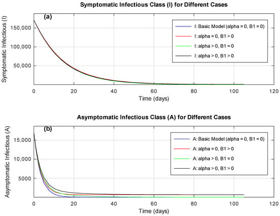
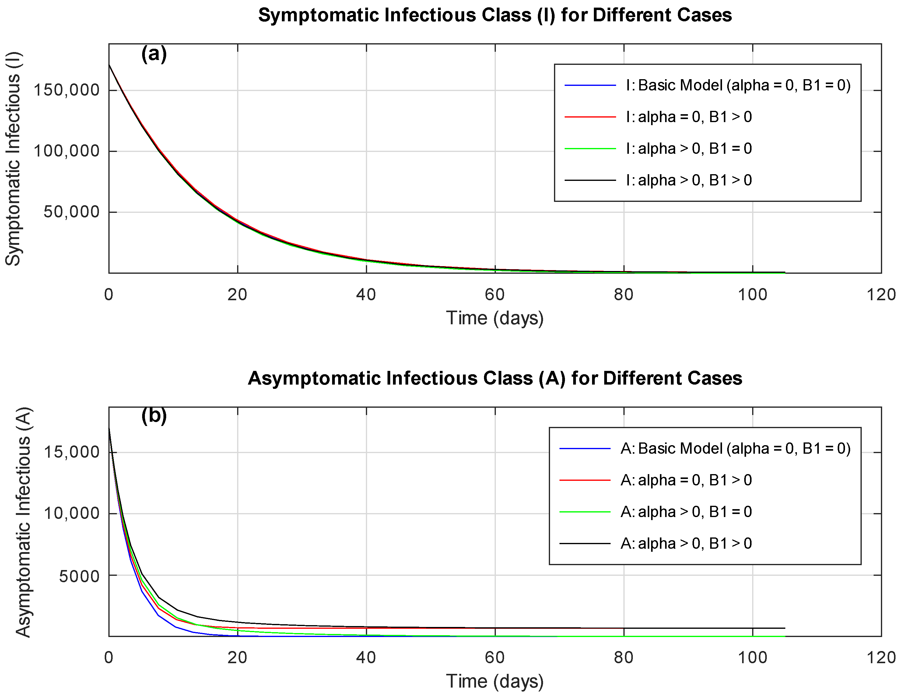
Figure 2 displays the development of symptomatic (I) and asymptomatic (A) infectious individuals over time across four different scenarios: the original model and three modified versions.

Figure 2. Time evolution of symptomatic (I) and asymptomatic (A) infectious classes for different model scenarios, spanning 105 days starting from 20 July 2020. Subfigure (a) shows symptomatic individuals, while subfigure (b) shows asymptomatic individuals. Symptomatic refers to individuals showing clinical symptoms, while asymptomatic refers to those infected but not exhibiting symptoms.

Figure 2a shows the number of symptomatic individuals (I) over time. From Day 0 to Day 30, all scenarios show a notable rise, with the steepest increase in Case 4 (black curve), where both $\alpha$ and $B_1$ are elevated, increasing the transmission rate. Case 1 (blue curve), the baseline scenario, exhibits the slowest growth and lowest peak. From Day 30 to Day 60, Case 4 maintains the highest peak, while Case 1 remains moderate. After Day 60, symptomatic cases decline across all scenarios, with Case 1 dropping off more sharply.

Figure 2b illustrates the trajectory of asymptomatic individuals (A). Although the shape of the curves is similar to those in Figure 2a, the number of asymptomatic infections is consistently lower. Again, Case 4 shows the highest peak and fastest rise, while Case 1 remains the lowest. These trends indicate that increasing both $\alpha$ and $B_1$ results in greater transmission among both symptomatic and asymptomatic groups.

It is important to note that the simulated ratio of asymptomatic to symptomatic infections ($A/I$) in our model is approximately 0.1, which reflects the context of South Africa during the first wave of the pandemic (20 July to 2 November 2020) [37]. At the time, the national testing strategy was largely symptom-based, prioritizing individuals showing clinical signs, known contacts, or those presenting to healthcare facilities [44]. Consequently, asymptomatic cases were likely underreported in real-world data. This limitation is mirrored in our model outputs. In contrast, countries such as Slovakia that implemented mass population screening were able to detect a greater number of asymptomatic infections, yielding an $A/I$ ratio closer to 1.0 [45]. The observed $A/I$ ratio in our model is therefore context-dependent and shaped by the testing strategies in place. However, the model is designed to be flexible and may be recalibrated for different epidemiological conditions or data environments.

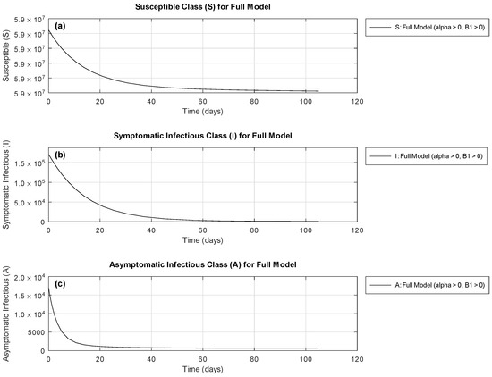
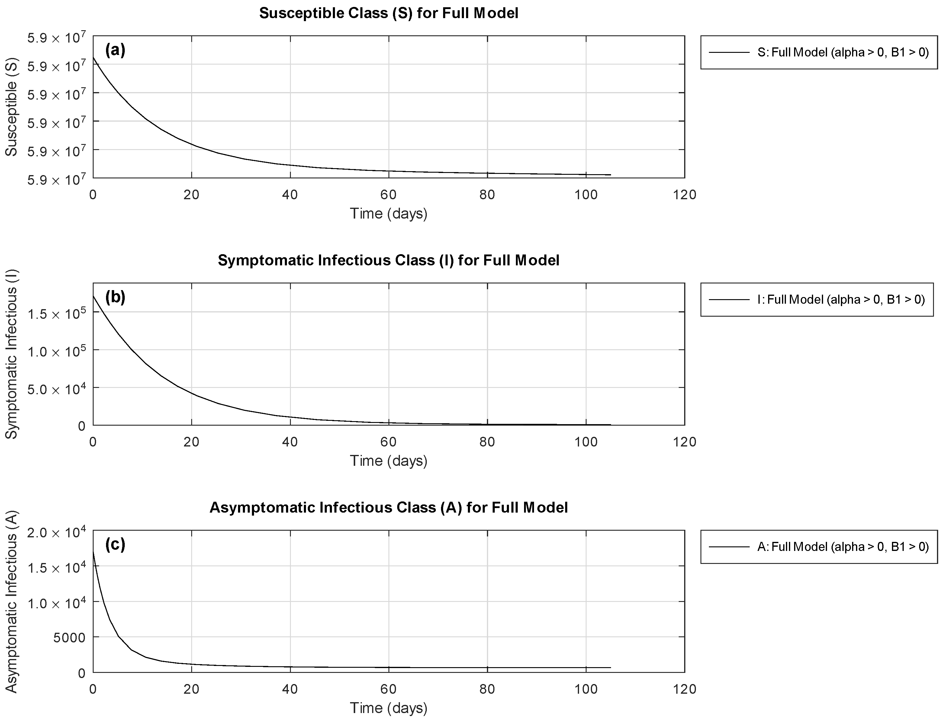
Figure 3 depicts the evolution of three categories; susceptible (S), symptomatic infectious (I), and asymptomatic infectious (A), over time for the complete model (Case 4), where both $\alpha >0$ and $B_1>0$ are active transmission parameters. The figure is organized into three subplots: (a) shows the decline in the susceptible class, (b) shows the symptomatic infections, and (c) displays the asymptomatic infections.

Figure 3. Evolution of susceptible (S), symptomatic infectious (I), and asymptomatic infectious (A) classes over 105 days starting from 20 July 2020 for Case 4 (with default values of $\alpha$ and $B_1$). Subfigure (a) shows the decline of susceptible individuals, subfigure (b) tracks the symptomatic infections, and subfigure (c) illustrates the asymptomatic infections.

In subplot (a), the susceptible population S declines steadily from Day 0 to Day 60, corresponding to the rate at which individuals move into infectious states. The decline begins to plateau afterward, suggesting reduced transmission due to a shrinking susceptible pool.

In subplot (b), the symptomatic infectious class I increases rapidly from Day 0 to around Day 45, where it peaks before beginning to decline. This reflects a surge in symptomatic cases driven by elevated $\alpha$ and $B_1$, followed by a natural resolution of infections as recovery or isolation occurs.

In subplot (c), the asymptomatic class A shows a similar trend, though with a lower magnitude and a more gradual increase. The delayed and lower peak indicates that asymptomatic spread remains present but less dominant, in line with the assumptions of the model.

Overall, the figure illustrates that higher values of $\alpha$ and $B_1$ contribute to faster spread and a higher infection burden, followed by stabilization as the epidemic evolves.

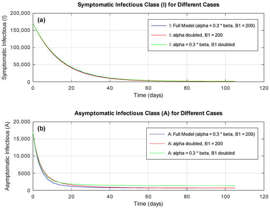
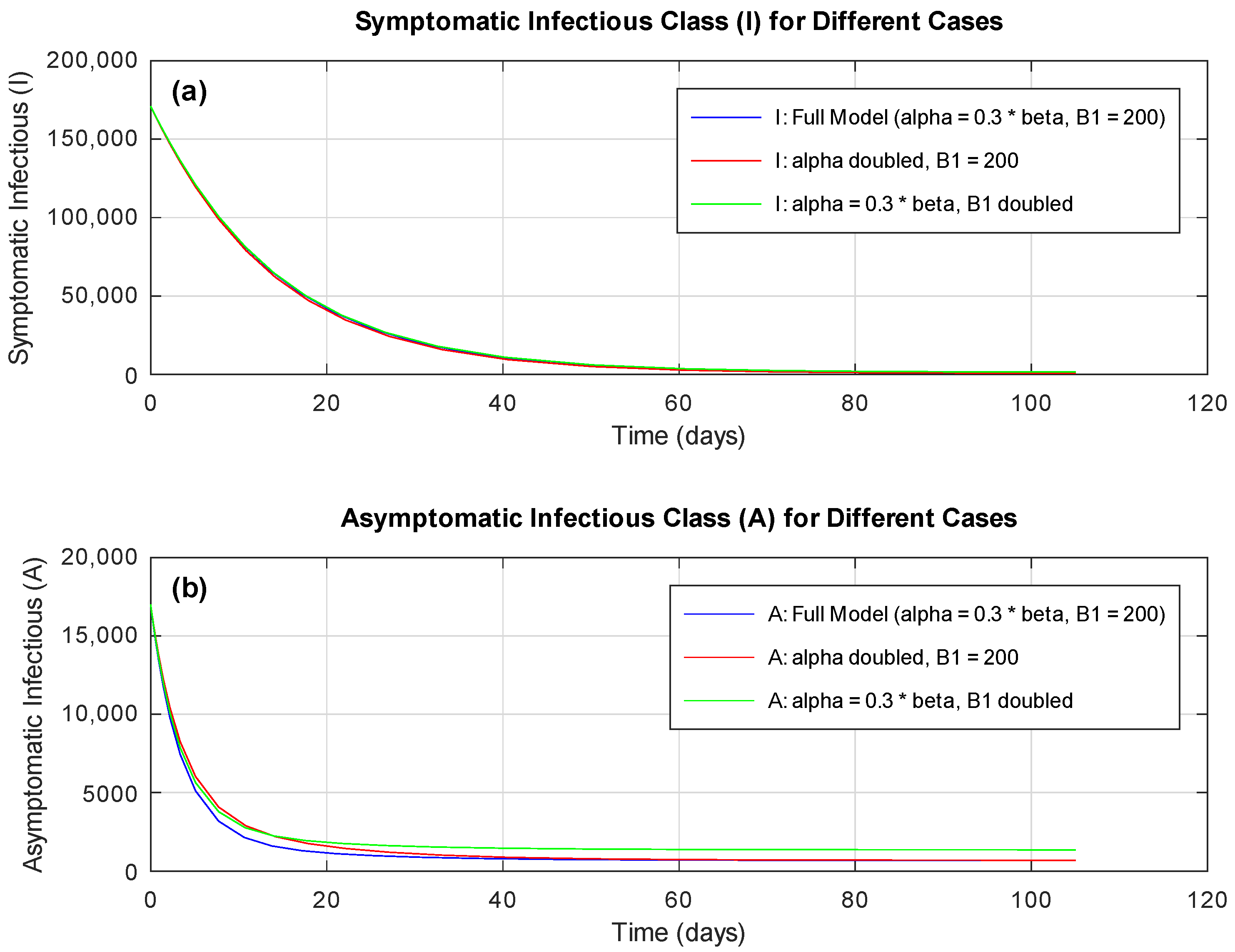
Figure 4 illustrates the dynamics of symptomatic (I) and asymptomatic (A) infectious classes over a period of 105 days under three distinct scenarios:

Figure 4. Changes in infection rates over time for three distinct combinations of $\alpha$ and $B_1$, spanning 105 days starting from 20 July 2020. Subplot (a): Symptomatic infectious individuals (I); (b): asymptomatic infectious individuals (A).

• Case 1: the full model ($\alpha =0.3\beta$, $B_1=200$, blue curve);
• Case 2: a model with doubled $\alpha$ ($\alpha =0.6\beta$, $B_1=200$, red curve);
• Case 3: a model with doubled $B_1$ ($\alpha =0.3\beta$, $B_1=400$, green curve).

In subplot (a), which tracks symptomatic infections (I), all three cases show an initial rise from Day 0 to Day 30. Case 2 exhibits the most rapid increase due to the higher $\alpha$, indicating increased transmission from asymptomatic individuals. Case 3 also shows a steeper climb than Case 1, driven by the elevated value of $B_1$, which enhances the contact or exposure rate. Case 1 demonstrates a slower and more moderate growth.

From Day 30 to Day 60, the symptomatic curves begin to diverge more clearly. Case 2 continues to rise, reaching the highest peak, while Case 3 levels off earlier but remains above Case 1. After Day 60, symptomatic infections begin to decline in all scenarios, with Case 1 showing the sharpest reduction, indicating a more gradual spread and faster resolution under baseline parameter values.

Subplot (b) shows the corresponding trends for asymptomatic infections (A). The qualitative patterns mirror those of the symptomatic class: Case 2 reaches the highest asymptomatic prevalence, followed by Case 3, then Case 1. The differences in magnitude are smaller, but the temporal dynamics are consistent. This suggests that increases in either $\alpha$ or $B_1$ elevate both symptomatic and asymptomatic transmission, though their impact on I appears more pronounced.

All in all, this figure highlights how variations in $\alpha$ and $B_1$ affect both the intensity and timing of the epidemic curve, with higher values leading to faster and more severe outbreaks.

9. Conclusions and Future Work

This study presents a comprehensive COVID-19 compartmental model that incorporates infective immigrants, asymptomatic transmission and environmental pathogen reservoirs, offering a more nuanced perspective on the disease’s dynamics than models focused solely on direct symptomatic spread. Rigorous theoretical analyses, including the existence and uniqueness of the endemic equilibrium (Theorems 2 and 3), confirmed via Descartes’ rule of signs, and the global stability of the disease-free equilibrium (Theorem 5), provide strong mathematical grounding for the model’s behavior across a range of epidemiological conditions.

Simulation results highlight the critical influence of key parameters, including the environmental transmission coefficient and the asymptomatic infectious rate, on shaping epidemic trajectories. While the asymptomatic-to-symptomatic ratio ($A/I$) used in this model reflects the testing context in South Africa during the first wave, where symptom-based testing led to likely underreporting of asymptomatic cases, this assumption was chosen deliberately to match available data. The model is flexible and can be recalibrated for alternative scenarios or settings with broader surveillance strategies.

These findings align with prior studies while extending them by quantifying the impact of environmental viral persistence and asymptomatic carriers, factors often underrepresented in earlier models. Public health interventions that focus solely on symptomatic individuals risk overlooking silent transmission drivers, thus, the model reinforces the importance of more comprehensive control strategies.

Nonetheless, the current model includes simplifying assumptions such as homogeneous mixing and static parameter values, which limit its ability to reflect population heterogeneity, adaptive behaviors, or changing conditions over time. Future work should focus on enhancing realism through the inclusion of time-varying parameters, vaccination dynamics, age-structured compartments, and heterogeneous contact networks. Incorporating these complexities would improve the model’s predictive utility and its applicability to real-time decision-making during future outbreaks.

By bridging rigorous mathematical analysis with epidemiological relevance, this work contributes to the understanding of COVID-19 transmission dynamics and underscores the importance of including hidden and environmental modes of transmission in pandemic modeling frameworks.

References

- Zhang, Y.-Y.; Li, B.-R.; Ning, B.-T. The comparative immunological characteristics of SARS-CoV, MERS-CoV, and SARS-CoV-2 coronavirus infections. Front. Immunol. 2020, 11, 2033. [Google Scholar] [CrossRef] [Scilit]
- Zhou, P.; Yang, X.L.; Wang, X.G.; Hu, B.; Zhang, L.; Zhang, W.; Si, H.R.; Zhu, Y.; Li, B.; Huang, C.L.; et al. A pneumonia outbreak associated with a new coronavirus of probable bat origin. Nature 2020, 579, 270–273. [Google Scholar] [CrossRef] [Scilit] [PubMed]
- Guan, W.-J.; Ni, Z.-Y.; Hu, Y.; Liang, W.-H.; Ou, C.-Q.; He, J.-X.; Liu, L.; Shan, H.; Lei, C.-l.; Hui, D.S.; et al. Clinical characteristics of coronavirus disease 2019 in China. N. Engl. J. Med. 2020, 382, 1708–1720. [Google Scholar] [CrossRef] [Scilit] [PubMed]
- Huang, C.; Wang, Y.; Li, X.; Ren, L.; Zhao, J.; Hu, Y.; Zhang, L.; Fan, G.; Xu, J.; Gu, X.; et al. Clinical features of patients infected with 2019 novel coronavirus in Wuhan, China. Lancet 2020, 395, 497–506. [Google Scholar] [CrossRef] [Scilit] [PubMed]
- Wiersinga, W.J.; Rhodes, A.; Cheng, A.C.; Peacock, S.J.; Prescott, H.C. Pathophysiology, transmission, diagnosis, and treatment of coronavirus disease 2019 (COVID-19): A review. JAMA 2020, 324, 782–793. [Google Scholar] [CrossRef] [Scilit]
- Nematswerani, N.; Steenkamp, L.; Haneef, S.; Naidoo, R.; Fonn, S. Understanding the impact of the COVID-19 pandemic on healthcare services for adults during three waves of COVID-19 infections: A South African private sector experience. S. Afr. Med. J. -Suid-Afr. Tydskr. Vir Geneeskd. 2023, 113, 1156–1164. [Google Scholar] [CrossRef] [Scilit]
- de Villiers, C.; Cerbone, D.; van Zijl, W. The South African government’s response to COVID-19. J. Public Budg. Account. Financ. Manag. 2020, 32, 797–811. [Google Scholar] [CrossRef] [Scilit]
- Perez, G.I.P.; Abadi, A.T.B. Ongoing challenges faced in the global control of COVID-19 pandemic. Arch. Med. Res. 2020, 51, 574–576. [Google Scholar] [CrossRef] [Scilit]
- McAleer, M. Prevention Is Better Than the Cure: Risk Management of COVID-19. J. Risk Financ. Manag. 2020, 13, 46. [Google Scholar] [CrossRef] [Scilit]
- Ahmed, S.F.; Quadeer, A.A.; McKay, M.R. Preliminary identification of potential vaccine targets for the COVID-19 coronavirus (SARS-CoV-2) based on SARS-CoV immunological studies. Viruses 2020, 12, 254. [Google Scholar] [CrossRef] [Scilit]
- McLean, G.; Kamil, J.; Lee, B.; Moore, P.; Schulz, T.F.; Muik, A.; Sahin, U.; Türeci, Ö.; Pather, S. The impact of evolving SARS-CoV-2 mutations and variants on COVID-19 vaccines. mBio 2022, 13, e02979-21. [Google Scholar] [CrossRef] [Scilit] [PubMed]
- Zhao, Z.; Bashiri, S.; Ziora, Z.M.; Toth, I.; Skwarczynski, M. COVID-19 variants and vaccine development. Viruses 2024, 16, 757. [Google Scholar] [CrossRef] [Scilit] [PubMed]
- Vellingiri, B.; Jayaramayya, K.; Iyer, M.; Narayanasamy, A.; Govindasamy, V.; Giridharan, B.; Ganesan, S.; Venugopal, A.; Venkatesan, D.; Ganesan, H.; et al. COVID-19: A promising cure for the global panic. Sci. Total Environ. 2020, 725, 138277. [Google Scholar] [CrossRef] [Scilit] [PubMed]
- Chi, W.Y.; Li, Y.D.; Huang, H.C.; Chan, T.E.H.; Chow, S.Y.; Su, J.H.; Ferrall, L.; Hung, C.F.; Wu, T.C. COVID-19 vaccine update: Vaccine effectiveness, SARS-CoV-2 variants, boosters, adverse effects, and immune correlates of protection. J. Biomed. Sci. 2022, 29, 82. [Google Scholar] [CrossRef] [Scilit]
- Luo, W.R.; Wu, X.M.; Wang, W.; Yu, J.L.; Chen, Q.Q.; Zhou, X.; Huang, X.; Pan, H.F.; Liu, Z.R.; Gao, Y.; et al. Novel coronavirus mutations: Vaccine development and challenges. Microb. Pathog. 2022, 173, 105828. [Google Scholar] [CrossRef] [Scilit]
- Slomski, A. Repurposed drugs failed to prevent severe COVID-19. JAMA 2022, 328, 1171. [Google Scholar] [CrossRef] [Scilit]
- Martinez, M.A. Efficacy of repurposed antiviral drugs: Lessons from COVID-19. Drug Discov. Today 2022, 27, 1954–1960. [Google Scholar] [CrossRef] [Scilit]
- Ford, N.; Vitoria, M.; Rangaraj, A.; Norris, S.L.; Calmy, A.; Doherty, M. Systematic review of the efficacy and safety of antiretroviral drugs against SARS, MERS or COVID-19: Initial assessment. J. Int. Aids Soc. 2020, 23, e25489. [Google Scholar] [CrossRef] [Scilit]
- Shah, B.; Modi, P.; Sagar, S.R. In silico studies on therapeutic agents for COVID-19: Drug repurposing approach. Life Sci. 2020, 252, 117652. [Google Scholar] [CrossRef] [Scilit]
- Chen, N.; Zhou, M.; Dong, X.; Qu, J.; Gong, F.; Han, Y.; Qiu, Y.; Wang, J.; Liu, Y.; Wei, Y.; et al. Epidemiological and clinical characteristics of 99 cases of 2019 novel coronavirus pneumonia in Wuhan, China: A descriptive study. Lancet 2020, 395, 507–513. [Google Scholar] [CrossRef] [Scilit]
- Andrews, N.; Stowe, J.; Kirsebom, F.; Toffa, S.; Rickeard, T.; Gallagher, E.; Gower, C.; Kall, M.; Groves, N.; O’Connell, A.M.; et al. COVID-19 vaccine effectiveness against the Omicron (B. 1.1. 529) variant. N. Engl. J. Med. 2022, 386, 1532–1546. [Google Scholar] [CrossRef] [Scilit]
- Zeng, B.; Gao, L.; Zhou, Q.; Yu, K.; Sun, F. Effectiveness of COVID-19 vaccines against SARS-CoV-2 variants of concern: A systematic review and meta-analysis. BMC Med. 2022, 20, 200. [Google Scholar] [CrossRef] [Scilit]
- Townsend, J.P.; Hassler, H.B.; Wang, Z.; Miura, S.; Singh, J.; Kumar, S.; Ruddle, N.H.; Galvani, A.P.; Dornburg, A. The durability of immunity against reinfection by SARS-CoV-2: A comparative evolutionary study. Lancet Microbe 2021, 2, e666–e675. [Google Scholar] [CrossRef] [Scilit]
- Stein, C.; Nassereldine, H.; Sorensen, R.J.; Amlag, J.O.; Bisignano, C.; Byrne, S.; Castro, E.; Coberly, K.; Collins, J.K.; Dalos, J.; et al. Past SARS-CoV-2 infection protection against re-infection: A systematic review and meta-analysis. Lancet 2023, 401, 833–842. [Google Scholar] [CrossRef] [Scilit] [PubMed]
- Simon, V.A. Long-Term Data Reveals SARS-CoV-2 Infection and Vaccine-Induced Antibody Responses Are Long-Lasting. Mount Sinai Newsroom, New York, 26 February 2024. Available online: https://www.mountsinai.org/about/newsroom/2024/longterm-data-reveals-sarscov2-infection-and-vaccineinduced-antibody-responses-are-longlasting (accessed on 10 July 2025).
- Srivastava, K.; Carreño, J.M.; Gleason, C.; Monahan, B.; Singh, G.; Abbad, A.; Tcheou, J.; Raskin, A.; Kleiner, G.; van Bakel, H.; et al. SARS-CoV-2-infection-and vaccine-induced antibody responses are long lasting with an initial waning phase followed by a stabilization phase. Immunity 2024, 57, 587–599. [Google Scholar] [CrossRef] [Scilit] [PubMed]
- Dangi, T.; Sanchez, S.; Lew, M.H.; Awakoaiye, B.; Visvabharathy, L.; Richner, J.M.; Koralnik, I.J.; Penaloza-MacMaster, P. Pre-existing immunity modulates responses to mRNA boosters. Cell Rep. 2023, 42, 112167. [Google Scholar] [CrossRef] [Scilit] [PubMed]
- Mwalili, S.; Kimathi, M.; Ojiambo, V.; Gathungu, D.; Mbogo, R. SEIR model for COVID-19 dynamics incorporating the environment and social distancing. BMC Res. Notes 2020, 13, 352. [Google Scholar] [CrossRef] [Scilit]
- Akingbade, J.A.; Ayegbusi, F.D. A Deterministic Mathematical Model and Analysis of Transmission Dynamics of COVID-19 from Reservoir-to-Human. Trends Comput. Appl. Math. 2025, 26, e01796. [Google Scholar] [CrossRef] [Scilit]
- Khan, T.; Rihan, F.A.; Riaz, M.B.; Altanji, M.; Zaagan, A.A.; Ahmad, H. Stochastic epidemic model for the dynamics of novel coronavirus transmission. AIMS Math. 2024, 9, 12433–12457. [Google Scholar] [CrossRef] [Scilit]
- Assan, B.; Nyabadza, F. A COVID-19 epidemic model with periodicity in transmission and environmental dynamics. Front. Appl. Math. Stat. 2023, 9, 1142625. [Google Scholar] [CrossRef] [Scilit]
- Cesari, L. Optimization-Theory and Applications: Problems with Ordinary Differential Equations; Springer: New York, NY, USA, 2012; Volume 17, p. XIV-542. [Google Scholar] [CrossRef] [Scilit]
- Maku Vyambwera, S.; Witbooi, P. A Stochastic TB Model for a Crowded Environment. J. Appl. Math. 2018, 2018, 3420528. [Google Scholar] [CrossRef] [Scilit]
- Witbooi, P.J.; Africa, C.; Christoffels, A.; Ahmed, I.H.I. A population model for the 2017/18 listeriosis outbreak in South Africa. PLoS ONE 2020, 15, e0229901. [Google Scholar] [CrossRef] [Scilit] [PubMed]
- Worldometer. South African Population in 2020. Available online: https://www.worldometers.info/world-population/south-africa-population/ (accessed on 1 September 2022).
- Witbooi, P.J. An SEIR model with infected immigrants and recovered emigrants. Adv. Differ. Equ. 2021, 2021, 337. [Google Scholar] [CrossRef] [Scilit] [PubMed]
- World Health Organization. South African Population Timeline from 20 July 2020 Until 2 November 2020. Available online: https://covid19.who.int/region/afro/country/za (accessed on 31 August 2022).
- Witbooi, P.J.; Vyambwera, S.M.; Nsuami, M.U. Control and elimination in an SEIR model for the disease dynamics of COVID-19 with vaccination. AIMS Math. 2023, 8, 8144–8161. [Google Scholar] [CrossRef] [Scilit]
- Tilahun, G.; Demie, S.; Eyob, A. Stochastic model of measles transmission dynamics with double dose vaccination. Infect. Dis. Model. 2020, 5, 478–494. [Google Scholar] [CrossRef] [Scilit]
- Vyambwera, S.M.; Witbooi, P. A two-group model of TB in a crowded environment. Appl. Math. Inf. Sci. 2021, 15, 523–532. [Google Scholar] [CrossRef] [Scilit]
- Affi Osei, P. Sensitivity Analysis of the SEIR Epidemic Compartment Model. Int. J. Sci. Res. (IJSR) 2018, 7, 352–357. Available online: https://api.semanticscholar.org/CorpusID:202705453 (accessed on 17 April 2025).
- van den Driessche, P.; Watmough, J. Reproduction numbers and sub-threshold endemic equilibria for compartmental models of disease transmission. Math. Biosci. 2002, 180, 29–48. [Google Scholar] [CrossRef] [Scilit]
- Lyapunov, A.M. The general problem of the stability of motion. Int. J. Control 1992, 55, 531–534. [Google Scholar] [CrossRef] [Scilit]
- Baxter, C.; Abdool Karim, Q.; Abdool Karim, S.S. Identifying SARS-CoV-2 infections in South Africa: Balancing public health imperatives with saving lives. Biochem. Biophys. Res. Commun. 2021, 538, 221–225. [Google Scholar] [CrossRef] [Scilit]
- Reuters. Mass Coronavirus Testing in Slovakia. Second Round. 7 November 2020. Available online: https://www.voanews.com/covid-19-pandemic/slovakias-second-round-coronavirus-tests-draws-large-crowds (accessed on 20 June 2025).
Disclaimer/Publisher’s Note: The statements, opinions and data contained in all publications are solely those of the individual author(s) and contributor(s) and not of MDPI and/or the editor(s). MDPI and/or the editor(s) disclaim responsibility for any injury to people or property resulting from any ideas, methods, instructions or products referred to in the content. |
© 2026 by the authors. Licensee MDPI, Basel, Switzerland. This article is an open access article distributed under the terms and conditions of the Creative Commons Attribution (CC BY) license.