The Junction of PDEs, Financial Mathematics and Probability: Deriving Classical and Generalized Black-Scholes–Merton Formulas

Abstract

This paper explores the intersection of three foundational areas—partial differential equations, financial mathematics, and probability—by providing a rigorous framework for the classical Black-Scholes–Merton option pricing model and its generalized extensions. For the classical model, a change in variables is employed to transform the Black-Scholes partial differential equation into the linear heat equation. The resulting formulation enables the use of Fourier transform techniques and the fundamental solution (heat kernel) to derive the closed-form Black-Scholes–Merton formula. To extend the classical setting, the interest rate in the discount factor and the stock’s rate of return are modeled using a multifactor Vasicek process, leading to a more sophisticated and realistic option pricing framework. In addition, a complementary derivation based on probabilistic methods, using a change in measure, yields an alternative explicit pricing formula. Numerical experiments based on Monte Carlo simulation show excellent agreement with the closed-form solutions and illustrate notable gains in computational efficiency. The comparative analysis further demonstrates that stochastic interest rates systematically produce lower option prices than the classical constant-rate model, underscoring the importance of accurate interest-rate modeling in practical valuation.

1. Introduction

This paper investigates the well-known Black-Scholes partial differential equation, which characterizes the evolution of derivative prices under the Black-Scholes model [1]. Developed by Fischer Black and Myron Scholes in 1973, this model became the first widely adopted framework for option pricing and remains one of the most significant applications of Itô calculus in financial engineering. The equation determines the fair value of a European-style call option based on observable market quantities—such as the current asset price, maturity, and strike price—under a set of structural assumptions on asset price dynamics.

The model lies at the intersection of three fundamental areas: partial differential equations, financial mathematics, and probability theory. It belongs to the theory of PDEs because the option price satisfies a second-order parabolic differential equation; it is central to mathematical finance due to its role in describing option price dynamics and it relies on probability since its solution involves the lognormal distribution. Furthermore, through appropriate transformations, the Black-Scholes equation can be converted into the classical heat equation, revealing a deep analogy between option price evolution and heat diffusion.

The model assumes that asset prices follow a geometric Brownian motion with constant volatility and interest rates, and that markets are frictionless, with no transaction costs or taxes. Although real markets often deviate from these idealized assumptions, the Black-Scholes framework remains a cornerstone of modern finance, with numerous extensions developed to address its limitations. In its classical formulation, the option value depends on five principal inputs: the current asset price, strike price, time to maturity, risk-free interest rate, and volatility.

The derivation of the Black-Scholes PDE is based on constructing a risk-free portfolio consisting of a long position in the option and a short position in the underlying asset, applying Itô’s lemma to the option price, and eliminating stochastic terms using the principle of no arbitrage. This procedure models the asset price via geometric Brownian motion, analyzes the change in the hedging portfolio, and equates its return to that of a risk-free investment (see [1,2]).

Once the pricing PDE is established, the natural question concerns the methods available to solve it. Broadly, option pricing techniques fall into two major categories: analytical approaches (see [3,4,5,6,7]) and numerical methods (see [8,9]). These include closed-form analytical solutions, finite-difference schemes, Fourier methods, stochastic simulation techniques, and modern approaches such as machine learning and neural-network-based solvers (see [10]), each accompanied by its own mathematical formulation.

A central mathematical question concerns the existence and uniqueness of solutions to the Black-Scholes PDE. Following the original ideas of Black and Scholes, the option price may be formulated as a terminal-value problem for a parabolic partial differential equation. Thus, PDE theory provides a natural and rigorous framework for option pricing. We refer interested readers to [1] and the references therein for a comprehensive discussion.

Beyond the classical constant-interest-rate setting, this paper further extends the model by incorporating stochastic interest rates through a multifactor Vasicek process. In [11], the single-factor Hull–White model (a generalization of the Vasicek model) is highlighted for its widespread industry use, particularly in pricing basket options with nonzero correlation between the interest rate process and multiple asset factors. Motivated by the literature (see [12,13,14,15]), we advance this framework by adopting a multifactor structure to capture richer and more realistic interest rate dynamics.

In this generalized setting, deriving explicit formulas for call and put option prices relies on fundamental probabilistic tools, including change in measure and change in numéraire. Meanwhile, PDE techniques reappear naturally in the pricing of zero-coupon bonds, as the interest rate is no longer constant.

In summary, this paper examines the analytic structure of the Black-Scholes–Merton pricing formula and explores how methods from partial differential equations, mathematical finance, and probability interact in both the classical constant-rate model and its stochastic-rate extension. The structure of the paper is as follows. Section 2 presents the classical derivation of the Black-Scholes PDE. Section 3 discusses well-posedness and the construction of solutions. Section 4 develops the generalized Black-Scholes–Merton pricing formula under stochastic interest rates. Section 5 provides numerical results and related discussion.

2. Black-Scholes PDEs

In the Black-Scholes model, the stock price behaves as a geometric Brownian motion, so that the evolution of the value of the asset, denoted by $S_t$ (see [16,17]), in continuous time is given by the following stochastic differential equation

$$d{S}_t=\mu S_{t}dt+\sigma S_{t}d{W}_t$$

(1)

where $\mu$ is the drift rate, $\sigma$ is the volatility, and $W_t$ is a Wiener process. Let us recall that the Wiener process $W={\left(W_t\right)}_{t\ge 0}$ is a real-valued continuous stochastic process, also known as a standard Brownian motion. It is characterized by the following properties:

• $W_t=0$ almost surely.
• W has independent increments: for every $t>0,$ the future increments $W_{t+s}-W_t,s\ge 0,$ are independent of the past values $W_s,0\le s\le t.$
• W has Gaussian increments: $W_{t+s}-W_t$ is normally distributed with mean 0 and variance s; that is, $W_{t+s}-W_t\sim \mathcal{N}(0,s).$
• W has continuous paths: $W_t$ is continuous in t.

According to [18], stocks and options are combined to create a replication portfolio. The return on the portfolio, assuming risk neutrality, is equal to the risk-free rate. Applying Itô’s Lemma to the option value, V depending on $S_t$ and t, we obtain the following:

$$\begin{array}{c}\hfill dV={\displaystyle \frac{\partial V}{\partial t}}dt+{\displaystyle \frac{\partial V}{\partial S}}d{S}_t+{\displaystyle \frac{1}{2}}{\displaystyle \frac{{\partial }^{2}V}{\partial S^2}}{\left(d{S}_t\right)}^2,\end{array}$$

(2)

for all $t\in [0,T)$ and $S\ge 0$.

Substituting the Equation (1) for $d{S}_t$ into the Equation (2) and under the assumption of risk neutrality, the return on the portfolio is the risk-free rate. The Black-Scholes PDE or Black-Scholes–Merton PDE for the option value $V(t,S_t)$, is defined as follows:

$$\begin{array}{c}\hfill {\displaystyle \frac{\partial V}{\partial t}}+{\displaystyle \frac{1}{2}}{\sigma }^2{S}_t^2{\displaystyle \frac{{\partial }^{2}V}{\partial S^2}}+r{S}_t{\displaystyle \frac{\partial V}{\partial S}}-rV=0,\mathrm{for}\mathrm{all}t\in [0,T),S\ge 0,\end{array}$$

(3)

that is, the Black-Scholes equation is a PDE in t and $S_t$, and it holds for any derivative with arbitrary $f\left(S_T\right)$ at a fixed time $t=T$, and the derivative price function $V(t,S_t)$ needs to be twice differentiable with respect to $S_t$ and once differentiable with respect to t. The drift $\mu$ of the underlying price movement does not appear in the Black-Scholes equation and hence, the price of any derivative will be independent of the expected rate of return of the underlying. However, take note of the appearance of the underlying volatility $\sigma$ and the riskless rate of return r in the Black-Scholes equation. In this study, the parameters $\sigma$ and r are positive constant, which makes implementation straightforward and we investigate the case of European call and put options, whose payoff functions are $max(S_T-K,0)$ and $max(K-S_T,0)$, respectively, where K denotes the strike price and $S_T$ is the price of the underlying asset at the maturity date T. Let us denote the function value V by C and P for European call and put options, respectively.

The term ${\displaystyle \frac{\partial V}{\partial t}}$ in the Equation (3) is the rate of change in the option price with respect to time, known as “$\Theta$”, $\begin{array}{c}\hfill {\displaystyle \frac{\partial V}{\partial S}}\end{array}$ is the rate of change in the option value with respect to the underlying stock price, known as “$\Delta$”, and $\begin{array}{c}\hfill {\displaystyle \frac{{\partial }^{2}V}{\partial S^2}}\end{array}$ is the rate of change in the $\Delta$ option with respect to the underlying stock price, known as “$\Gamma$”. In the financial context, the Black-Scholes PDE is highlighted by the following decomposition of its right hand side

$$\begin{array}{c}\hfill \underset{\mathrm{portfolio} \mathrm{return}}{\underbrace{{\displaystyle \frac{\partial V}{\partial t}}+{\displaystyle \frac{1}{2}}{\sigma }^2{S}_t^2{\displaystyle \frac{{\partial }^{2}V}{\partial S^2}}}}-\underset{\mathrm{bank} \mathrm{investment}}{\underbrace{r\left(V-S_t{\displaystyle \frac{\partial V}{\partial S}}\right).}}\end{array}$$

We will denote $\mathcal{B}$ the differential operator

$$\begin{array}{c}\hfill \mathcal{B}V={\displaystyle \frac{1}{2}}{\sigma }^2{S}_t^2{\displaystyle \frac{{\partial }^{2}V}{\partial S^2}}+r{S}_t{\displaystyle \frac{\partial V}{\partial S}}-rV,\end{array}$$

so that the Black-Scholes Equation (3) is described concisely as

$${\displaystyle \frac{\partial V}{\partial t}}(t,S_t)+\mathcal{B}V(t,S_t)=0$$

To obtain the well-posedness of the Black-Scholes PDE, see [19], we need a final condition at $t=T$ and boundary conditions at $S_t=0$ and as $S_t\to +\infty$.

• Final conditions. We first examine the conditions that must be imposed at time $t=T$.
  For a call option, if at time T we have $S_T>K$, then we exercise the option with a profit of $S_T-K$. If $S_T\le K$, we do not exercise the option and obtain no profit. Therefore, the final payoff of the call option is

  $$C(T,S_T)=max(S_T-K,0)={(S_T-K)}^{+},S_T>0.$$
  For a put option, if at time T we have $S_T\ge K$, then we do not exercise the option, while if $S_T<K$, we exercise it. Thus, the final payoff of the put option is

  $$P(T,S_T)=max(K-S_T,0)={(K-S_T)}^{+},S_T>0.$$
• Boundary conditions. We now examine the conditions to be imposed at $S_t=0$ and as $S_t\to +\infty$.
  Call option. If $S_0=0$, then $S_t=0$ for any $t\ge 0$, and the option has no value. Hence,

  $$C(t,0)=0,t\ge 0.$$
  As $S_t\to +\infty$ at time t, the option becomes deep in the money and will end up in the money at maturity. The payoff of the call option is

  $$C(T,S_T)={(S_T-K)}^{+}\to S_T-K,\mathrm{as}{S}_T\to +\infty .$$
  Thus, the present value at time t approaches the risk-neutral expectation of $e^{-r(T-t)}(S_T-K)$, which is equivalent to

  $$C(t,S_t)-(S_t-K{e}^{-r(T-t)})\to 0\mathrm{as}{S}_t\to +\infty ,\mathrm{for}\mathrm{fixed}t.$$
  Put option. If $S_0=0$, then $S_t=0$ for $t\ge 0$, and the payoff of the put option is

  $$P(T,S_T)={(K-S_T)}^{+}=K.$$
  Therefore, the present value at time t is the discounted value of K:

  $$P(t,S_t)=K{e}^{-r(T-t)}.$$
  If $S_t\to +\infty$, then the payoff is always zero, so the option is never exercised. Consequently, the present value of the put option satisfies

  $$P(t,S_t)=0\mathrm{as}{S}_t\to +\infty ,\mathrm{for}\mathrm{fixed}t.$$

In PDE terms, the Black-Scholes PDE can be viewed as

$${\displaystyle \frac{\partial u}{\partial t}}=a{x}^2{\displaystyle \frac{{\partial }^{2}u}{\partial x^2}}+bx{\displaystyle \frac{\partial u}{\partial x}}+cu,t,x>0$$

(4)

with $a=-{\displaystyle \frac{{\sigma }^2}{2}}, b=-r,$ and $c=r$ and $u=u(t,x)$ is the option price depending on the current value of the underlying asset x and time t.

By the classical theory of partial differential equations, the linear parabolic Equation (4) can be reduced to a heat equation

$${\displaystyle \frac{\partial v}{\partial t}}={\displaystyle \frac{{\partial }^{2}v}{\partial x^2}}$$

(5)

under a suitable change in variables. The solution of the heat Equation (5) can be obtained for any initial condition using the Fourier transform methods [19,20,21].

The primary goal is to explore the interrelation of the dynamic of the stock price from the perspective of probability; that is, the mathematical property of $S_t$ that follows the lognormal distribution. The classical method in partial differential equations, namely the Fourier transform, can be used to solve the heat equation. Once the solution of the heat equation is obtained, then the option price can easily be recovered for the Black-Scholes PDE, which models the dynamics of option pricing in financial mathematics.

3. Well-Posedness

In this section, we first provide the probability properties of the stock price $S_t$. Then, we investigate the well-posedness of the solution of the Black-Scholes PDE in the case of European call and put options.

Theorem 1.

The solution of the Equation (1) is given by

$$S_t=S_0{e}^{\left(\mu -{\displaystyle \frac{{\sigma }^2}{2}}\right)t+\sigma W_t},t>0.$$

(6)

Proof. 

In this proof, we will use the technique that has been addressed in [17]. First, we rewrite the Equation (1) in integral form as follows:

$$S_t=S_0+\mu {\int }_0^t{S}_{s}ds+\sigma {\int }_0^t{S}_{s}d{W}_s.$$

Applying Itô Lemma to $f\left(S_t\right)=ln\left(S_t\right)$ with $f\left(x\right)=lnx$, we obtain

$$\begin{array}{cc}\hfill dln\left(S_t\right)& =\mu S_t{f}^{\prime }\left(S_t\right)dt+\sigma S_t{f}^{\prime }\left(S_t\right)d{W}_t+{\displaystyle \frac{1}{2}}{\sigma }^2{S}_t^2{f}^{\prime \prime }\left(S_t\right)dt\hfill \\ \hfill & =\mu dt+\sigma d{W}_t-{\displaystyle \frac{1}{2}}{\sigma }^{2}dt\hfill \\ \hfill & =\left(\mu -{\displaystyle \frac{{\sigma }^2}{2}}\right)dt+\sigma d{W}_t\hfill \end{array}$$

Therefore,

$$\begin{array}{cc}\hfill ln\left(S_t\right)-ln\left(S_0\right)& ={\int }_0^{t}dln\left(S_u\right)\hfill \\ \hfill & ={\int }_0^t\left(\mu -{\displaystyle \frac{{\sigma }^2}{2}}\right)du+{\int }_0^t\sigma d{W}_u\hfill \\ \hfill & =\left(\mu -{\displaystyle \frac{{\sigma }^2}{2}}\right)t+\sigma W_t,t>0\hfill \end{array}$$

and it follows that

$$S_t=S_0{e}^{\left(\mu -{\displaystyle \frac{{\sigma }^2}{2}}\right)t+\sigma W_t},t>0.$$

    □

From the representation of $S_t$ in (6), we observe that the geometric Brownian motion provides a realistic model for stock price dynamics. In particular, (6) ensures that if $S_0>0$, then $S_t>0$ for all $t\in [0,T]$, which is consistent with real-world financial markets where stock prices cannot become negative.

Define

$$H_t=\left(\mu -{\displaystyle \frac{{\sigma }^2}{2}}\right)t+\sigma W_t,$$

which is a Brownian motion with drift. In this context, $H_t$ represents the continuous rate of return of the stock over the time interval $[0,t]$. Moreover, $H_t$ corresponds to the logarithmic growth of the stock price, since

$$H_t=ln\left({\displaystyle \frac{S_t}{S_0}}\right).$$

Thus, the random variable $H_t$ is normally distributed with mean $\left(\mu -{\displaystyle \frac{{\sigma }^2}{2}}\right)t$ and variance ${\sigma }^{2}t$. Hence, its probability density function is given by

$$\begin{array}{c}\hfill f_{H_t}\left(y\right)={\displaystyle \frac{1}{\sqrt{2\pi {\sigma }^{2}t}}}exp\left\{-{\displaystyle \frac{{(y-(\mu -\frac{{\sigma }^2}{2})t)}^2}{2{\sigma }^{2}t}}\right\}.\end{array}$$

By leveraging the representation of $S_t$ in (6), the following proposition provides the explicit form of the probability density function of $S_t$ as well as its expectation and variance.

Proposition 1.

The density of $S_t$ is given by

$$f_{S_t}\left(s\right)={\displaystyle \frac{1}{s\sqrt{2\pi {\sigma }^{2}t}}}exp\left\{-{\displaystyle \frac{{\left(ln\left(\frac{s}{S_0}\right)-\left(\mu -\frac{{\sigma }^2}{2}\right)t\right)}^2}{2{\sigma }^{2}t}}\right\},$$

which is called the lognormal density. Furthermore, the expectation and variance of $S_t$ are given by

$$\begin{array}{cc}\hfill \mathbb{E}\left(S_t\right)& =S_0{e}^{\mu t},\hfill \\ \hfill \mathbb{V}\left(S_t\right)& ={\left(S_0{e}^{\mu t}\right)}^2\left(e^{{\sigma }^{2}t}-1\right).\hfill \end{array}$$

Proof. 

A detailed proof of this proposition is provided in [17,22]. □

Now, we consider the European call option with strike price K with the option value $C(t,S_t)$ and the boundary condition given by the payoff function $C(T,S_T)=max(S_T-K,0)$. The Black-Scholes PDE reads

$$\left\{\begin{array}{c}{\displaystyle \frac{\partial C}{\partial t}}+{\displaystyle \frac{1}{2}}{\sigma }^2{S}_t^2{\displaystyle \frac{{\partial }^{2}C}{\partial S^2}}+r{S}_t{\displaystyle \frac{\partial C}{\partial S}}-rC=0\hfill \\ C(T,S_T)=max(S_T-K,0)\hfill \\ C(t,0)=0\hfill \\ C(t,S_t)-(S_t-K{e}^{-r(T-t)})\to 0\mathrm{as}{S}_t\to +\infty ,\mathrm{for}\mathrm{fixed}t.\hfill \end{array}\right.$$

(7)

To ensure the existence and uniqueness of the solution to (7), in addition to assuming that $C(t,S_t)$ is twice continuously differentiable with respect to the stock price S and once continuously differentiable with respect to time t, we also impose a linear growth condition on $C(t,S_t)$. Specifically, we require that

$$|C(t,S_t)| \le N(1+S_t),$$

for all $t\in [0,T]$, where N is a positive constant. For more details on the concepts of existence and uniqueness for parabolic partial differential equations, see [21,23].

Problems involving partial differential equations usually arise in the form of initial value problems, where the boundary conditions specify the state of some system at time $t=0$, and we wish to determine the behavior of the system for $t>0.$ In contrast, the Black-Scholes PDE (together with the boundary conditions) gives as a final value problem the following: We want to determine $C(t,S_t)$ for $0\le t<T$ given the value $C(T,S_T)$ at the maturity date T. We point out that the coefficient of $\begin{array}{c}\hfill {\displaystyle \frac{{\partial }^{2}C}{\partial S^2}}\end{array}$ is positive so that the Equation (7) is a backward equation, and it is reasonable to introduce a chance of time variable $\tau =T-t$ to reverse the progression of time, such that we look forward for C rather than backwards (since we know the price at maturity T), so that we have an initial value problem, where C is known at time $\tau =0$ and we are interested in the behavior of C for $\tau >0$. Recall that the stock price follows the lognormal distribution; that motivates the change in the variable of the logarithm of the stock price as follows

$$x={\displaystyle \frac{1}{\sigma }}\left[ln\left(S_t\right)+\left(r-{\displaystyle \frac{{\sigma }^2}{2}}\right)\tau \right].$$

This removes the $S_t$ coefficient in front of $\begin{array}{c}\hfill {\displaystyle \frac{{\partial }^{2}C}{\partial S^2}}\end{array}$ term and eliminates the $\begin{array}{c}\hfill {\displaystyle \frac{\partial C}{\partial S}}\end{array}$ term entirely, and the transformation

$$u(\tau ,x)=C(t,S_t)e^{r\tau }$$

leads to the heat equation form. We have the following result that transform Black-Scholes PDE into a classical heat equation.

Theorem 2.

With the change-of-variables transformations

$$\tau =T-t,x={\displaystyle \frac{1}{\sigma }}\left[ln\left(S_t\right)+\left(r-{\displaystyle \frac{{\sigma }^2}{2}}\right)\tau \right],u(\tau ,x)=C(t,S_t)e^{r\tau },$$

(8)

the PDE (7) reduces into the heat equation

$$\left\{\begin{array}{c}{\displaystyle \frac{\partial u}{\partial \tau }}={\displaystyle \frac{1}{2}}{\displaystyle \frac{{\partial }^{2}u}{\partial x^2}}\hfill \\ u(0,x)=max\left(e^{\sigma x}-K,0\right),x\in \mathbb{R}.\hfill \end{array}\right.$$

(9)

Proof. 

As already stated, the option price $C(t,S_t)$ is twice continuously differentiable with respect to the stock price S and once continuously differentiable with respect to time. Hence, from (8), the transformed function u also possesses these properties. Moreover, under the assumption of linear growth of the option price, the transformed function u likewise inherits this property.

Since

$$t=T-\tau ,S_t=e^{\sigma x+\left({\displaystyle \frac{{\sigma }^2}{2}}-r\right)\tau }$$

we have

$${\displaystyle \frac{\partial t}{\partial \tau }}=-1,\begin{array}{c}\hfill {\displaystyle \frac{\partial S_t}{\partial \tau }}=\left({\displaystyle \frac{{\sigma }^2}{2}}-r\right)S_t\end{array},{\displaystyle \frac{\partial S_t}{\partial x}}=\sigma S_t.$$

Applying the chain rule, we have the first derivative of u with respect to time $\tau ,$

$$\begin{array}{cc}\hfill {\displaystyle \frac{\partial u}{\partial \tau }}& ={\displaystyle \frac{\partial C}{\partial \tau }}(t,S_t)e^{r\tau }+{\displaystyle \frac{\partial e^{r\tau }}{\partial \tau }}C(t,S_t)\hfill \\ \hfill & =r{e}^{r\tau }C(t,S_t)+e^{r\tau }\left({\displaystyle \frac{\partial C}{\partial t}}(t,S_t){\displaystyle \frac{\partial t}{\partial \tau }}+{\displaystyle \frac{\partial C}{\partial S}}(t,S_t){\displaystyle \frac{\partial S_t}{\partial \tau }}\right)\hfill \\ \hfill & =r{e}^{r\tau }C(t,S_t)+e^{r\tau }\left(-{\displaystyle \frac{\partial C}{\partial t}}(t,S_t)+\left({\displaystyle \frac{{\sigma }^2}{2}}-r\right)S_t{\displaystyle \frac{\partial C}{\partial S}}(t,S_t)\right)\hfill \\ \hfill & =r{e}^{r\tau }C(t,S_t)-e^{r\tau }{\displaystyle \frac{\partial C}{\partial t}}(t,S_t)+\left({\displaystyle \frac{{\sigma }^2}{2}}-r\right)e^{r\tau }{S}_t{\displaystyle \frac{\partial C}{\partial S}}(t,S_t)\hfill \\ \hfill & ={\displaystyle \frac{1}{2}}{\sigma }^2{S}_t^2{e}^{r\tau }{\displaystyle \frac{{\partial }^{2}C}{\partial S^2}}+{\displaystyle \frac{{\sigma }^2}{2}}{e}^{r\tau }{S}_t{\displaystyle \frac{\partial C}{\partial S}}(t,S_t),\hfill \end{array}$$

(10)

for $t\in [0,T)$ and $S\ge 0$. On the last step we used the Black-Scholes PDE. On the other hand, we have the first and second derivative of u with respect to $x,$

$${\displaystyle \frac{\partial u}{\partial x}}=\sigma S_t{e}^{r\tau }{\displaystyle \frac{\partial C}{\partial S}}(t,S_t)$$

and

$$\begin{array}{cc}\hfill {\displaystyle \frac{1}{2}}{\displaystyle \frac{{\partial }^{2}u}{\partial x^2}}& ={\displaystyle \frac{1}{2}}{\displaystyle \frac{\partial }{\partial x}}\left(e^{r\tau }\sigma S_t{\displaystyle \frac{\partial C}{\partial S}}(t,S_t)\right)\hfill \\ \hfill & ={\displaystyle \frac{1}{2}}{e}^{r\tau }\sigma \left({\displaystyle \frac{\partial S_t}{\partial x}}{\displaystyle \frac{\partial C}{\partial S}}(t,S_t)+S_t{\displaystyle \frac{\partial }{\partial x}}\left({\displaystyle \frac{\partial C}{\partial S}}(t,S_t)\right)\right)\hfill \\ \hfill & ={\displaystyle \frac{1}{2}}\sigma e^{r\tau }\left(\sigma S_t{\displaystyle \frac{\partial C}{\partial S}}(t,S_t)+S_t^2{\displaystyle \frac{{\partial }^{2}C}{\partial S^2}}(t,S_t)\right)\hfill \\ \hfill & ={\displaystyle \frac{{\sigma }^2}{2}}{e}^{r\tau }{S}_t{\displaystyle \frac{\partial C}{\partial S}}(t,S_t)+{\displaystyle \frac{1}{2}}{\sigma }^2{S}_t^2{e}^{r\tau }{\displaystyle \frac{{\partial }^{2}C}{\partial S^2}},\hfill \end{array}$$

(11)

for $t\in [0,T)$ and $S\ge 0$.

We conclude by comparing (10) and (11), which shows that $u(\tau ,x)$ solves the heat Equation (9). When $S_t$ goes from 0 to $+\infty$, x varies from $-\infty$ to $+\infty$. When $t=T$ we have $\tau =0$. Then the initial condition of (9) is

$$u(0,x)=C(T,S_T)=max\left(e^{\sigma x}-K,0\right).$$

The other two boundary conditions become

$$u(\tau ,x)\to 0\mathrm{as}x\to -\infty ,u(\tau ,x)\to e^{r\tau }\left(e^{\sigma x+\left({\displaystyle \frac{{\sigma }^2}{2}}-r\right)\tau }-K\right)\mathrm{as}x\to +\infty .$$

    □

Theorem 2 allows us to solve the Black-Scholes PDE (7) to obtain the Black-Scholes formula systematically for the European call and put options based on the solution of the heat equation defined in Equation (9) and by the relation

$$\tau =T-t,x={\displaystyle \frac{1}{\sigma }}\left[ln\left(S_t\right)+\left(r-{\displaystyle \frac{{\sigma }^2}{2}}\right)\tau \right],$$

That is,

$$C(t,S_t)=e^{-r(T-t)}u\left(T-t,{\displaystyle \frac{1}{\sigma }}\left[ln\left(S_t\right)+\left(r-{\displaystyle \frac{{\sigma }^2}{2}}\right)(T-t)\right]\right).$$

It is well established that the Cauchy problem associated with the heat Equation (9) admits a smooth solution (see [20,21,23]). This fundamental result ensures that the heat equation is well-posed in the classical sense. Consequently, because the Black-Scholes partial differential equation can be transformed into the heat equation through an appropriate change in variables, the well-posedness of the heat equation immediately guarantees the well-posedness of the Black-Scholes equation.

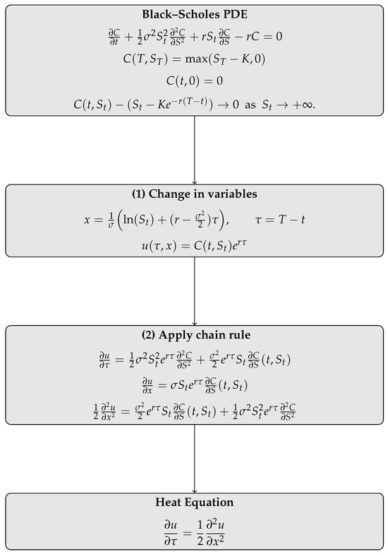
To facilitate comprehension and to make the transformation from the Black-Scholes PDE to the heat equation as transparent as possible, we present below Figure 1: a schematic diagram that illustrates the correspondence step by step. This visual representation is intended to guide the reader through the analytic connection between the two formulations.

Figure 1. A schematic diagram illustrating the transformation from the Black-Scholes PDE defined in (7) to the heat equation defined in (9).

Next, we focus on the heat equation defined in Equation (9) (see [21] for more detail about heat equation). In the classical PDE context, $u(\tau ,x)$ represents the temperature of an infinite metal rod at the point x at time $\tau$ and $u(0,x)$ denotes the initial temperature. We also assume that no heat enters or leaves the rod, so that the total amount of heat in the rod is constant (i.e., does not vary with time). With appropriate scaling, we may assume this constant is 1. We thus impose the condition

$${\int }_{-\infty }^{+\infty }u(\tau ,x)dx=1.$$

As time progresses, heat will dissipate from warmer regions to cooler regions, so that the temperature distribution gradually evens out. We will see how solutions of the heat equation can be built up systematically.

We begin the heat equation with a very special boundary condition: we consider the situation where at time 0 all the heat is concentrated at the point $x=0$. The boundary condition is thus

$$u(0,x)=\delta \left(x\right),$$

where $\delta$ represents the Dirac delta function, defined as follows:

$$\delta \left(x\right)=0,\mathrm{if}x\ne 0,{\int }_{-\infty }^{+\infty }\delta \left(x\right)dx=1.$$

Remark 1.

The Dirac delta function is not a function in the strict mathematical sense, as it cannot be determined by simply assigning a value to each x. Instead, it is a generalized function or distribution, which is determined by integrating over the entire real line and multiplying by an appropriate test function.

Here, we wish to determine the fundamental solution of the heat equation. We will use the mathematical tool called the Fourier transform to establish such a solution. To do this, if u is smooth which, along with all derivatives, decay rapidly at infinity, or, in general, if u is a tempered distribution (for a formal definition of tempered distribution, see [20]), one defines $\widehat{u}\left(\xi \right)$ the Fourier transform of u by

$$\mathcal{F}\left(u\right)\left(\xi \right):=\widehat{u}\left(\xi \right):={\int }_{-\infty }^{+\infty }u\left(x\right)e^{-ix\xi }dx,\mathrm{where}{i}^2=-1,$$

(12)

and the inverse Fourier transform by

$${\mathcal{F}}^{-1}\left(\widehat{u}\right)\left(x\right):=u\left(x\right)={\displaystyle \frac{1}{2\pi }}{\int }_{-\infty }^{+\infty }\widehat{u}\left(\xi \right)e^{ix\xi }d\xi .$$

It follows that the Fourier transform of the $\delta$ function is given by

$$\widehat{\delta }\left(\xi \right)={\int }_{-\infty }^{+\infty }\delta \left(x\right)e^{-ix\xi }dx=e^{-i·0·\xi }=1.$$

We highlight some important properties of the Fourier transform that are required in what follows.

Proposition 2.

The following properties hold for all $\xi \in \mathbb{R},$

1.

$$\widehat{(au+v)}\left(\xi \right)=a\widehat{u}\left(\xi \right)+\widehat{v}\left(\xi \right),a\in \mathbb{R}.$$

2.

$$\widehat{{\displaystyle \frac{du}{dx}}}\left(\xi \right)=i\xi \widehat{u}\left(\xi \right).$$

3.

$$\widehat{xu}\left(\xi \right)=i{\displaystyle \frac{d\widehat{u}}{d\xi }}\left(\xi \right).$$

Proof. 

The proof of this proposition can be found in [20]. □

The following result shows that the Fourier transform of a Gaussian is Gaussian, which is essential when we wish to determine the fundamental solution of the heat equation.

Proposition 3.

For $a>0,$

$$\widehat{\left(e^{-a{x}^2}\right)}\left(\xi \right)=\sqrt{{\displaystyle \frac{\pi }{a}}}{e}^{-{\displaystyle \frac{{\xi }^2}{4a}}}.$$

Proof. 

The proof of this proposition is followed directly by the formula of the Fourier transform defined in (12) together with its properties that are stated in Proposition 3. A detail of this proof can be found in [20,21]. □

Note that Proposition 3 yields

$${\mathcal{F}}^{-1}\left(e^{-{\displaystyle \frac{{\xi }^2}{4a}}}\right)\left(x\right)=\sqrt{{\displaystyle \frac{a}{\pi }}}{e}^{-a{x}^2}.$$

Similarly, assume that with respect to the x variable, u is smooth, which, along with all derivatives, decay rapidly at infinity, one defines $\widehat{u}(\tau ,\xi )$ the Fourier transform of $u(\tau ,x)$ in the x variable; that is,

$$\mathcal{F}\left(u(\tau ,.)\right)\left(\xi \right):=\widehat{u}(\tau ,\xi ):={\int }_{-\infty }^{+\infty }u(\tau ,x)e^{-ix\xi }dx,$$

together with its partial inverse Fourier transform

$${\mathcal{F}}^{-1}\left(\widehat{u}(\tau ,.)\right)\left(x\right):=u(\tau ,x)={\displaystyle \frac{1}{2\pi }}{\int }_{-\infty }^{+\infty }\widehat{u}(\tau ,x)e^{ix\xi }d\xi .$$

The following Fourier transform properties play a vital role in establishing the fundamental solution of the heat equation. These properties are as follows:

1.

The Fourier transform of the partial time derivatives of $u(\tau ,x)$ is the partial time derivative of $\widehat{u}(\tau ,\xi )$.

2.

The Fourier transform of the spatial derivatives of $u(\tau ,x)$ is the product of the factor $\left(i\xi \right)$ and $\widehat{u}(\tau ,\xi )$.

Proposition 4.

The following properties hold for all $\xi \in \mathbb{R},$

1.

$$\widehat{{\displaystyle \frac{\partial u}{\partial \tau }}}(\tau ,\xi )={\displaystyle \frac{\partial \widehat{u}}{\partial \tau }}(\tau ,\xi ).$$

2.

$$\widehat{{\displaystyle \frac{\partial u}{\partial x}}}(\tau ,\xi )=i\xi \widehat{u}(\tau ,\xi ).$$

3.

$$\widehat{{\displaystyle \frac{{\partial }^{2}u}{\partial x^2}}}(\tau ,\xi )=-{\xi }^2\widehat{u}(\tau ,\xi ).$$

Proof. 

The proof of this proposition can be found in [20]. □

Theorem 3.

The fundamental solution of the heat equation

$$\left\{\begin{array}{c}{\displaystyle \frac{\partial u}{\partial \tau }}={\displaystyle \frac{1}{2}}{\displaystyle \frac{{\partial }^{2}u}{\partial x^2}}\hfill \\ u(0,x)=\delta \left(x\right),\hfill \end{array}\right.$$

is given by the Gaussian probability density function

$$u_{\delta }(t,x):={\displaystyle \frac{1}{\sqrt{2\pi \tau }}}{e}^{-{\displaystyle \frac{x^2}{2\tau }}},x\in \mathbb{R},$$

with a variance $\tau >0.$

Proof. 

Let $\widehat{u}(\tau ,\xi )$ be the Fourier transform of $u(\tau ,x)$ in the x variable; that is,

$$\widehat{u}(\tau ,\xi )={\int }_{-\infty }^{+\infty }u(\tau ,x)e^{-ix\xi }dx.$$

We take the Fourier transform on (9) and using Proposition 4 to obtain

$$\begin{array}{cc}\hfill \widehat{{\displaystyle \frac{\partial u}{\partial \tau }}}(\tau ,\xi )& ={\displaystyle \frac{1}{2}}\widehat{{\displaystyle \frac{{\partial }^{2}u}{\partial x^2}}}(\tau ,\xi )\hfill \\ \hfill {\displaystyle \frac{\partial \widehat{u}}{\partial \tau }}(\tau ,\xi )& =-{\displaystyle \frac{1}{2}}{\xi }^2\widehat{u}(\tau ,\xi ).\hfill \end{array}$$

The solution of this ordinary differential equation for a fixed $\xi$ in $\mathbb{R}$ is

$$\widehat{u}(\tau ,\xi )=\widehat{u}(0,\xi )e^{-{\displaystyle \frac{1}{2}}\tau {\xi }^2}=\widehat{\delta }\left(\xi \right)e^{-{\displaystyle \frac{1}{2}}\tau {\xi }^2}=e^{-{\displaystyle \frac{1}{2}}\tau {\xi }^2}.$$

Therefore, the fundamental solution $u_{\delta }$ is given by the inverse Fourier transform and Proposition 3 as follows,

$$u_{\delta }(\tau ,x)={\mathcal{F}}^{-1}\left(e^{-{\displaystyle \frac{1}{2}}\tau {\xi }^2}\right)\left(x\right)={\displaystyle \frac{1}{\sqrt{2\pi \tau }}}{e}^{-{\displaystyle \frac{x^2}{2\tau }}}.$$

 □

The fundamental solution $u_{\delta }(\tau ,x)$ of the heat equation can be used to build a solution that satisfies any initial condition $u(0,x)=u_0\left(x\right).$ To do this, we need another important result in Fourier analysis, called “convolution theorem”, which turns the convolution of functions into the product of individual Fourier transforms. The convolution of f and g is written as $f\ast g$, denoting the operator with the symbol ”∗”, defined as follows:

$$(f\ast g)\left(x\right):={\int }_{-\infty }^{+\infty }f\left(y\right)g(x-y)dy,$$

(13)

provided the integral exists.

Proposition 5.

Assuming all integrals in the equation below exist, one has

$$\widehat{f\ast g}\left(\xi \right)=\widehat{f}\left(\xi \right)\widehat{g}\left(\xi \right).$$

Proof. 

The proof of the convolution theorem follows directly from the definition of convolution given in (13), together with the definition of the Fourier transform in (12). A detailed exposition of this argument can be found in [20]. □

Theorem 4.

The heat Equation (9) has a unique solution given by

$$\begin{array}{c}\hfill u(\tau ,x)={\int }_{-\infty }^{+\infty }u(0,z)e^{-{\displaystyle \frac{{(x-z)}^2}{2\tau }}}{\displaystyle \frac{dz}{\sqrt{2\pi \tau }}},x\in \mathbb{R},\tau >0.\end{array}$$

(14)

Proof. 

In this proof, we employ the result of Theorem 3 on the fundamental solution of the heat equation (the heat kernel), together with the convolution property stated in Proposition 5, in order to derive the general solution of the heat equation.

We follow the same line as in the proof of Theorem 3; we obtain the general solution of the heat Equation (9) of the form

$$\widehat{u}(\tau ,\xi )=\widehat{u}(0,\xi )e^{-{\displaystyle \frac{1}{2}}\tau {\xi }^2}.$$

By Proposition 3, we see that

$$e^{-{\displaystyle \frac{1}{2}}\tau {\xi }^2}={\displaystyle \frac{1}{\sqrt{2\pi \tau }}}\widehat{\left(e^{-{\displaystyle \frac{x^2}{2\tau }}}\right)}\left(\xi \right)={\widehat{u}}_{\delta }(\tau ,\xi ).$$

This implies that $\widehat{u}$ can be written as

$$\begin{array}{c}\hfill \widehat{u}(\tau ,\xi )=\widehat{u}(0,\xi ){\widehat{u}}_{\delta }(\tau ,\xi )=\widehat{u(0,.)\ast u_{\delta }(\tau ,.)}\left(\xi \right).\end{array}$$

It follows by taking the inverse Fourier transform and from the definition of convolution that

$$\begin{array}{cc}\hfill u(\tau ,x)& =(u(0,.)\ast u_{\delta }(\tau ,.))\left(x\right)\hfill \\ & ={\int }_{-\infty }^{+\infty }u(0,z)u_{\delta }(\tau ,x-z)dz\hfill \\ \hfill & ={\int }_{-\infty }^{+\infty }u(0,z)e^{-{\displaystyle \frac{{(x-z)}^2}{2\tau }}}{\displaystyle \frac{dz}{\sqrt{2\pi \tau }}}.\hfill \end{array}$$

This completes the proof. □

Finally, we are ready to establish the Black-Scholes formula for the European call option from the solution of the Black-Scholes PDE (7) as follows.

Theorem 5.

The solution of the PDE (7) is given by the Black-Scholes formula for call options

$$\begin{array}{c}\hfill C(t,S_t)=S_t\Phi \left(d_1\right)-K{e}^{-r(T-t)}\Phi \left(d_2\right),\end{array}$$

(15)

where $\Phi (.)$ is the cumulative distribution function of a standard normal distribution with mean zero and standard deviation of one. Here,

$$d_1={\displaystyle \frac{ln\left(\frac{S_t}{K}\right)+\left(r+\frac{1}{2}{\sigma }^2\right)(T-t)}{\sigma \sqrt{T-t}}},$$

and

$$d_2={\displaystyle \frac{ln\left(\frac{S_t}{K}\right)+\left(r-\frac{1}{2}{\sigma }^2\right)(T-t)}{\sigma \sqrt{T-t}}}=d_1-\sigma \sqrt{T-t},$$

for $0\le t<T.$

Proof. 

With the change in variables in Theorem 2,

$$\tau =T-t,x={\displaystyle \frac{1}{\sigma }}\left[ln\left(S_t\right)+\left(r-{\displaystyle \frac{{\sigma }^2}{2}}\right)\tau \right],$$

we obtain

$$C(t,S_t)=e^{-r(T-t)}u\left(T-t,{\displaystyle \frac{1}{\sigma }}\left[ln\left(S_t\right)+\left(r-{\displaystyle \frac{{\sigma }^2}{2}}\right)(T-t)\right]\right),$$

and

$$u(0,x)=max(e^{\sigma x}-K,0).$$

By Theorem 4, we obtain

$$\begin{array}{cc}\hfill C(t,S_t)& =e^{-r(T-t)}{\int }_{-\infty }^{+\infty }u\left(0,{\displaystyle \frac{1}{\sigma }}\left[ln\left(S_t\right)+\left(r-{\displaystyle \frac{{\sigma }^2}{2}}\right)(T-t)\right]+z\right)e^{-{\displaystyle \frac{z^2}{2(T-t)}}}{\displaystyle \frac{dz}{\sqrt{2\pi (T-t)}}}\hfill \\ \hfill & =e^{-r(T-t)}{\int }_{-\infty }^{+\infty }max\left(e^{ln\left(S_t\right)+\left(r-{\displaystyle \frac{{\sigma }^2}{2}}\right)(T-t)+\sigma z}-K,0\right)\times e^{-{\displaystyle \frac{z^2}{2(T-t)}}}{\displaystyle \frac{dz}{\sqrt{2\pi (T-t)}}}\hfill \\ \hfill & =e^{-r(T-t)}{\int }_{-\infty }^{+\infty }max\left(S_t{e}^{\left(r-{\displaystyle \frac{{\sigma }^2}{2}}\right)(T-t)+\sigma z}-K,0\right)e^{-{\displaystyle \frac{z^2}{2(T-t)}}}{\displaystyle \frac{dz}{\sqrt{2\pi (T-t)}}}.\hfill \end{array}$$

The integrand

$$\begin{array}{c}\hfill max\left(S_t{e}^{\left(r-{\displaystyle \frac{{\sigma }^2}{2}}\right)(T-t)+\sigma z}-K,0\right)e^{-{\displaystyle \frac{z^2}{2(T-t)}}}\end{array}$$

is positive if and only if

$$\begin{array}{c}\hfill z>{\displaystyle \frac{ln\left(\frac{K}{S_t}\right)-\left(r-\frac{{\sigma }^2}{2}\right)(T-t)}{\sigma }}\end{array}$$

which implies

$$\begin{array}{cc}\hfill C(t,S_t)& =e^{-r(T-t)}{\int }_{{\displaystyle \frac{ln\left(\frac{K}{S_t}\right)-\left(r-\frac{{\sigma }^2}{2}\right)(T-t)}{\sigma }}}^{+\infty }\left(S_t{e}^{\left(r-{\displaystyle \frac{{\sigma }^2}{2}}\right)(T-t)+\sigma z}-K\right)e^{-{\displaystyle \frac{z^2}{2(T-t)}}}{\displaystyle \frac{dz}{\sqrt{2\pi (T-t)}}}\hfill \\ \hfill & =S_t{\int }_{-d_2\sqrt{T-t}}^{+\infty }{e}^{-{\displaystyle \frac{{(z-\sigma (T-t))}^2}{2(T-t)}}}{\displaystyle \frac{dz}{\sqrt{2\pi (T-t)}}}\hfill \\ \hfill & -K{e}^{-r(T-t)}{\int }_{-d_2\sqrt{T-t}}^{+\infty }{e}^{-{\displaystyle \frac{z^2}{2(T-t)}}}{\displaystyle \frac{dz}{\sqrt{2\pi (T-t)}}}.\hfill \end{array}$$

(16)

By applying the change in variable on the integral (16), then we obtain

$$\begin{array}{cc}\hfill C(t,S_t)& =S_t{\int }_{-d_2\sqrt{T-t}-\sigma (T-t)}^{+\infty }{e}^{-{\displaystyle \frac{z^2}{2(T-t)}}}{\displaystyle \frac{dz}{\sqrt{2\pi (T-t)}}}\hfill \\ \hfill & -K{e}^{-r(T-t)}{\int }_{-d_2\sqrt{T-t}}^{+\infty }{e}^{-{\displaystyle \frac{z^2}{2(T-t)}}}{\displaystyle \frac{dz}{\sqrt{2\pi (T-t)}}}\hfill \\ \hfill & =S_t\left(1-\Phi (-d_1)\right)-K{e}^{-r(T-t)}\left(1-\Phi (-d_2)\right)\hfill \\ \hfill & =S_t\Phi \left(d_1\right)-K{e}^{-r(T-t)}\Phi \left(d_2\right).\hfill \end{array}$$

 □

Remark 2.

We now have an explicit solution to the Black-Scholes PDE, which provides the price of a European call option at any time t before the maturity date T. The formula expresses the option price in terms of the original financial variables, and involves the cumulative standard normal distribution Φ.

We check that the formula does indeed satisfy the boundaries condition for the European call option. We observe the limit of $C(t,S_t)$ as $t\to T$. If $S_t>K,$ then $ln(S_t/K)>0$ and both $d_1$ and $d_2$ tend to $+\infty$ as $t\to T$. This implies that $\Phi \left(d_1\right)$ and $\Phi \left(d_2\right)$ tend to 1 as $t\to T$. Hence, $C(t,S_t)\to S_T-K$. On the other hand, if $S_t<K,$ then $d_1$ and $d_2$ tend to $-\infty$ as $t\to T$, so that $C(t,S_t)\to 0$ as $t\to T$. Combining the two cases, we have $C(t,S_t)\to max(S_T-K,0)$ as $t\to T$. For the other two boundary conditions: as $S_t\to 0$ for fixed $t<T$, we have $d_1,d_2\to -\infty ,$ and $C(t,S_t)\to 0$ and as $S_t\to +\infty$, we have $C(t,S_t)\to S_t-K{e}^{-r(T-t)}.$

Similarly, in the case of the European put option with strike price K with the option value $P(t,S_t)$ and the boundary condition given by the payoff function $P(T,S_T)=max(K-S_T,0)$. The Black-Scholes PDE reads

$$\left\{\begin{array}{c}{\displaystyle \frac{\partial P}{\partial t}}+{\displaystyle \frac{1}{2}}{\sigma }^2{S}_t^2{\displaystyle \frac{{\partial }^{2}P}{\partial S^2}}+r{S}_t{\displaystyle \frac{\partial P}{\partial S}}-rP=0\hfill \\ P(T,S_T)=max(K-S_T,0).\hfill \end{array}\right.$$

(17)

Theorem 6.

The solution of the PDE (17) is given by the Black-Scholes formula for put options

$$P(t,S_t)=K{e}^{-r(T-t)}\Phi (-d_2)-S_t\Phi (-d_1),$$

(18)

with

$$d_1={\displaystyle \frac{ln\left(\frac{S_t}{K}\right)+\left(r+\frac{1}{2}{\sigma }^2\right)(T-t)}{\sigma \sqrt{T-t}}}$$

and

$$d_2={\displaystyle \frac{ln\left(\frac{S_t}{K}\right)+\left(r-\frac{1}{2}{\sigma }^2\right)(T-t)}{\sigma \sqrt{T-t}}}$$

for $0\le t<T.$

Proof. 

The proof follows directly from the principle of call–put parity, a foundational result in option pricing theory. This relationship, which establishes a precise equivalence between the values of European call and put options, has been extensively documented in classical references, including [17]. Accordingly, the argument presented here is an immediate consequence of this well-established parity condition.

$$\begin{array}{c}\hfill C(t,S_t)-P(t,S_t)=S_t-K{e}^{-r(T-t)},0\le t<T\end{array}.$$

(19)

Substituting (15) of Theorem 5 into (19), we observe that

$$\begin{array}{cc}\hfill P(t,S_t)& =C(t,S_t)-S_t+K{e}^{-r(T-t)}\hfill \\ \hfill & =K{e}^{-r(T-t)}(1-\Phi \left(d_2\right))-S_t(1-\Phi \left(d_1\right))\hfill \\ \hfill & =K{e}^{-r(T-t)}\Phi (-d_2)-S_t\Phi (-d_1),\hfill \end{array}$$

which is our desired formula. This completes the proof. □

Remark 3.

The Black-Scholes formula for the European put option can be found by applying the fundamental solution of the heat equation, with the same computation as the European call option.

Remark 4.

For the Black-Scholes model for a European call and a put option on stock paying a continuous dividend at rate δ. The Black-Scholes PDE is given by

$$\begin{array}{c}\hfill {\displaystyle \frac{\partial V}{\partial t}}+{\displaystyle \frac{1}{2}}{\sigma }^2{S}_t^2{\displaystyle \frac{{\partial }^{2}V}{\partial S^2}}+(r-\delta )S_t{\displaystyle \frac{\partial V}{\partial S}}-(r-\delta )V=0,t\in [0,T),S\ge 0,\end{array}$$

(20)

together with initial and boundary conditions depend on where it is call or put options.

The PDE (20) is exactly the same initial boundary value problem we have previously solved except r has been replaced by $r-\delta .$ It follows that the analytic solution of the PDE (20) can be established via the fundamental solution of the corresponding heat equation. Their solutions are given by the formulas

$$\begin{array}{cc}\hfill V^{\mathit{call}}(t,S_t)& =e^{-\delta (T-t)}{S}_t\Phi \left(d\right)-K{e}^{-r(T-t)}\Phi (d-\sigma \sqrt{T-t})\hfill \\ \hfill V^{\mathit{put}}(t,S_t)& =K{e}^{-r(T-t)}\Phi (\sigma \sqrt{T-t}-d)-e^{-\delta (T-t)}{S}_t\Phi (-d),\hfill \end{array}$$

where

$$d={\displaystyle \frac{ln\left(\frac{S_t}{K}\right)+\left(r-\delta +\frac{{\sigma }^2}{2}\right)(T-t)}{\sigma \sqrt{T-t}}}.$$

4. Generalized Black-Scholes–Merton Option Pricing Formula

In this part, we consider a generalized Black-Scholes–Merton option pricing framework in which the stock price process ${\left(S_t\right)}_{t\ge 0}$ satisfies the stochastic differential equation

$$d{S}_t=r_t{S}_{t}dt+{\sigma }^s{S}_{t}d{W}_t^s,t\in [0,T],T>0,$$

(21)

where ${\sigma }^s$ denotes the volatility and ${\left(W_t^s\right)}_{t\ge 0}$ is a Wiener process satisfying properties 1–4 on the probability space $(\Omega ,\mathcal{F},\mathbb{Q})$ with respect to the filtration ${\left({\mathcal{F}}_t\right)}_{t\ge 0}$. The drift term $r_t$ represents the short rate, defined by the following:

$$r_t=\sum _{j=1}^n{x}_t^{\left(j\right)},$$

(22)

where $n\ge 2$ and each factor process ${\left(x_t^{\left(j\right)}\right)}_{t\ge 0}$ is generated by the Vasicek SDE

$$d{x}_t^{\left(j\right)}=a^{\left(j\right)}\left(b^{\left(j\right)}-x_t^{\left(j\right)}\right)dt+{\sigma }^{\left(j\right)}d{W}_t^{\left(j\right)},x_0^{\left(j\right)}>0,$$

(23)

for $t\in [0,T]$, $T>0$, and $j=1,\dots ,n$. The parameters $a^{\left(j\right)},b^{\left(j\right)},{\sigma }^{\left(j\right)}$ are positive constants representing, respectively, the speed of mean reversion, the long-term mean level, and the instantaneous volatility.

Here, ${\left(W_t^{\left(j\right)}\right)}_{t\ge 0}$ denotes a Wiener process defined on the same risk-neutral probability space as ${\left(W_t^s\right)}_{t\ge 0}$ and adapted to the filtration ${\left({\mathcal{F}}_t\right)}_{t\ge 0}$. For $j=1,\dots ,n$, the Brownian motions ${\left(W_t^{\left(j\right)}\right)}_{t\ge 0}$ are mutually independent, satisfying

$$d{W}_t^{\left(i\right)}d{W}_t^{\left(j\right)}=0\mathrm{for}i\ne j,d{W}_t^{\left(j\right)}d{W}_t^{\left(j\right)}=dt.$$

Furthermore, each factor Brownian motion is correlated with the stock-price Brownian motion via

$$d{W}_t^{\left(j\right)}d{W}_t^s={\rho }_{j}dt,j=1,\dots ,n,$$

where ${\rho }_j$ denotes the correlation coefficient.

A key motivation for modeling the short rate $r_t$ using a multifactor Vasicek model is that, in practice, one-factor interest rate models are often insufficient to capture the full dynamics and fluctuations observed in real markets (see [12,13,14]). The Vasicek framework is widely used due to its mean-reversion property, as reflected in the drift term of (23). An additional advantage of the Vasicek model is its analytical tractability: the process $x_t^{\left(j\right)}$ admits a Gaussian transition density, which is generally unavailable for many alternative interest rate models (see [17,24]).

However, a well-known drawback of the Vasicek model is its allowance for negative interest rates, which may be inconsistent with certain market conditions.

Similar to Section 2, the payoff of a European call option at the maturity time T is defined as

$${\mathrm{Payoff}}_T=max(S_T-K,0)={(S_T-K)}^{+}.$$

(24)

The fair price of the call option is given by

$$C(t,x_t,S_t)={\mathbb{E}}^{\mathbb{Q}}\left[exp\left\{-{\int }_t^T\sum _{j=1}^n{x}_s^{\left(j\right)}ds\right\}{(S_T-K)}^{+}|{\mathcal{F}}_t\right],$$

(25)

for $t\in [0,T]$, where $x_t=(x_t^{\left(1\right)},\dots ,x_t^{\left(n\right)})\in {\mathbb{R}}_{+}$. Here, the option value is written as $C(t,x_t,S_t)$ to emphasize that it depends not only on the current stock price but also on the current levels of the interest-rate factors.

Since both the interest-rate processes and the stock price satisfy the Markov property, Equation (25) can be rewritten as

$$C(t,x,S_t)={\mathbb{E}}^{\mathbb{Q}}\left[exp\left\{-{\int }_t^T\sum _{j=1}^n{x}_s^{\left(j\right)}ds\right\}{(S_T-K)}^{+}|x_t=x,S_t\right],$$

(26)

for $t\in [0,T]$, $x=(x^{\left(1\right)},\dots ,x^{\left(n\right)})\in {\mathbb{R}}_{+}$, and $S_t>0$.

Since in this case the interest rate appearing in both the discount factor and the drift term of (21) is itself a stochastic process, and since its correlation with $S_T$ may be nonzero, computing the right-hand side of (26) becomes highly nontrivial.

Unlike Section 2, we will not rely on the PDE approach to derive the expression for $C(t,x,S_t)$. Instead, we employ the forward evolution method to eliminate the correlation between the interest rate and the stock price in the discount factor of (26) (see [11,17,25]).

To apply the forward evolution method, we first derive the present value of a zero-coupon bond under the multifactor Vasicek interest-rate model specified in (22) and (23).

A zero-coupon bond is a financial instrument that pays only its face value at maturity and generates no intermediate cash flows. Let $T>0$ denote the maturity date. Under the risk-neutral probability measure $\mathbb{Q}$, its price at time t with payoff $1 at T is given by

$$\overline{P}(t,x_t;T)={\mathbb{E}}^{\mathbb{Q}}\left[exp\left\{-{\int }_t^T{r}_{s}ds\right\}|{\mathcal{F}}_t\right]={\mathbb{E}}^{\mathbb{Q}}\left[exp\left\{-{\int }_t^T\sum _{j=1}^n{x}_s^{\left(j\right)}ds\right\}|{\mathcal{F}}_t\right],$$

(27)

for $t\in [0,T]$, where $x_t=(x_t^{\left(1\right)},\dots ,x_t^{\left(n\right)})\in {\mathbb{R}}_{+}$.

By the Markov property of the interest-rate factors, Equation (27) can be rewritten in the reduced form

$$\overline{P}(t,x;T)={\mathbb{E}}^{\mathbb{Q}}\left[exp\left\{-{\int }_t^T\sum _{j=1}^n{x}_s^{\left(j\right)}ds\right\}|x_t=x\right],$$

(28)

for $t\in [0,T]$ and $x=(x^{\left(1\right)},\dots ,x^{\left(n\right)})\in {\mathbb{R}}_{+}$.

By using the Feynman–Kac theorem, see [17], pages 268–272 for the Feynman–Kac theorem, the real-valued function $\overline{P}(t,x;T)$ with the dummy variables t and x can be derived by solving the following Cauchy problem:

$$\left\{\begin{array}{c}{\displaystyle \frac{\partial \overline{P}}{\partial t}}+{\displaystyle \frac{1}{2}}{\displaystyle \sum _{j=1}^n}{\left({\sigma }^{\left(j\right)}\right)}^2{\displaystyle \frac{{\partial }^2\overline{P}}{{(\partial x^{\left(j\right)})}^2}}+{\displaystyle \sum _{j=1}^n}(a^{\left(j\right)}{b}^{\left(j\right)}-a^{\left(j\right)}{x}^{\left(j\right)}){\displaystyle \frac{\partial \overline{P}}{\partial x^{\left(j\right)}}}-{\displaystyle \sum _{j=1}^n}{x}^{\left(j\right)}\overline{P}=0,\hfill \\ \overline{P}(T,x;T)=1.\hfill \end{array}\right.$$

(29)

In order to solve the Cauchy problem (29), we propose the following ansatz for the solution:

$$\overline{P}(t,x;T)=exp\left\{A(t;T)-\sum _{j=1}^n{B}_j(t;T)x^{\left(j\right)}\right\}.$$

(30)

The proposed solution (30) can be obtained because each process ${\left(x_t^{\left(j\right)}\right)}_{t\ge 0}$ is an affine process (see [26,27]).

Substituting (30) into (29), the Cauchy problem reduces to the following system of ordinary differential equations:

$$\left\{\begin{array}{cc}{\displaystyle \frac{d{B}_j}{dt}}\hfill & =a^{\left(j\right)}{B}_j-1,\hfill \\ {\displaystyle \frac{dA}{dt}}\hfill & ={\displaystyle \sum _{j=1}^n}{a}^{\left(j\right)}{b}^{\left(j\right)}{B}_j-{\displaystyle \frac{1}{2}}{\displaystyle \sum _{j=1}^n}{\left({\sigma }^{\left(j\right)}\right)}^2{B}_j^2,\hfill \end{array}\right.$$

(31)

subject to the terminal condition,

$$A(T;T)=B_j(T;T)=0,$$

(32)

for $t\in [0,T]$ and $j=1,\dots ,n$.

The real-valued functions $A(t;T)$ and $B_j(t;T)$ can be derived from (31) and (32) as follows:

$$\left\{\begin{array}{cc}{B}_j(t;T)\hfill & ={\displaystyle \frac{1-exp\{-a^{\left(j\right)}(T-t)\}}{a^{\left(j\right)}}},\hfill \\ A(t;T)\hfill & ={\displaystyle \sum _{j=1}^n}\left(b^{\left(j\right)}-{\displaystyle \frac{1}{2}}{\displaystyle \frac{{\left({\sigma }^{\left(j\right)}\right)}^2}{{\left(a^{\left(j\right)}\right)}^2}}\right)(B_j(t;T)-(T-t))-{\displaystyle \sum _{j=1}^n}{\displaystyle \frac{{\left({\sigma }^{\left(j\right)}\right)}^2}{4a^{\left(j\right)}}}{B}_j{(t;T)}^2,\hfill \end{array}\right.$$

(33)

for $t\in [0,T]$.

Remark 5.

If the parameters $a^{\left(j\right)}$, $b^{\left(j\right)}$, and ${\sigma }^{\left(j\right)}$, for $j=1,\dots ,n$, are time-dependent functions, say $a^{\left(j\right)}\left(t\right)$, $b^{\left(j\right)}\left(t\right)$, and ${\sigma }^{\left(j\right)}\left(t\right)$, then (23) is called a Hull–White model, which has been widely used in industrial settings. In this case, the zero-coupon bond price remains in the form of (30), but the real-valued functions $A(t;T)$ and $B_j(t;T)$ are given by the following:

$$\left\{\begin{array}{cc}{B}_j(t;T)\hfill & ={\int }_t^T{e}^{-{\int }_t^s{a}^{\left(j\right)}\left(u\right)du}ds,\hfill \\ A(t;T)\hfill & ={\displaystyle \sum _{j=1}^n}{\int }_t^T(a^{\left(j\right)}\left(s\right)b^{\left(j\right)}\left(s\right)B_j(s;T)-{\displaystyle \frac{1}{2}}{\left({\sigma }^{\left(j\right)}\left(s\right)\right)}^2{B}_j(s;T))ds,\hfill \end{array}\right.$$

(34)

for $t\in [0,T]$ and $j=1,\dots ,n$.

From the Equation (34), we observe that in most cases with time-dependent parameters, the explicit formulas of $A(t;T)$ and $B_j(t;T)$ are difficult to obtain. To overcome this issue, numerical integration can be applied to compute the value of the zero-coupon bond price.

To derive the explicit formula for the call option value $C(t,x,S_t)$ defined in (26), we do not employ the PDE approach. Instead, we rely on a probabilistic method. The main tool used in this derivation is a change of probability measure.

First, from the expression of the forward price of the stock given by

$${\mathrm{For}}_S(t;T)={\displaystyle \frac{S_t}{\overline{P}(t,x;T)}},$$

(35)

we will show that it is a martingale under the T-forward probability measure, a property that will play a crucial role in the proof of Theorem 7 below.

Proposition 6.

Under the T-forward measure with the relation

$${\displaystyle \frac{d{\tilde{\mathbb{P}}}^T}{d\mathbb{Q}}}{|}_{{\mathcal{F}}_t}={\displaystyle \frac{1}{\overline{P}(t,x;T)}}exp\left\{-{\int }_t^T\sum _{j=1}^n{x}_s^{\left(j\right)}ds\right\},$$

the forward price ${\mathit{For}}_S(t;T)$ defined in (35), is a martingale process and satisfies

$$d{\mathit{For}}_S(t;T)=\widehat{\sigma }\left(t\right){\mathit{For}}_S(t;T)d{\tilde{W}}_t^T,$$

(36)

where

$$\widehat{\sigma }\left(t\right)=\sqrt{{\left({\sigma }^s\right)}^2+2{\sigma }^s{\displaystyle \sum _{j=1}^n}{\rho }_j{\sigma }^{\left(j\right)}{B}_j(t;T)+{\displaystyle \sum _{j=1}^n}{\left({\sigma }^{\left(j\right)}\right)}^2{B}_j^2(t;T)}$$

(37)

and ${\left({\tilde{W}}_t^T\right)}_{t\ge 0}$ is a Brownian motion used to drive under the T-forward measure ${\tilde{\mathbb{P}}}^T$.

Before we go to prove the Proposition 6, we need to use some results in the following lemma.

Lemma 1.

Let $N_t$ be a strictly positive price process for a non-dividend-paying asset, either primary or derivative in the multidimensional market model. Then there exists a vector volatility process

$$\nu \left(t\right)=({\nu }_1\left(t\right),\cdots ,{\nu }_n\left(t\right))$$

such that

$$dN\left(t\right)=r_{t}N\left(t\right)dt+N\left(t\right)\nu \left(t\right)·d{W}_t,$$

(38)

where $W_t=(W_t^{\left(1\right)},\cdots ,W_t^{\left(n\right)})$.

This equation is equivalent to each of the equations

$$\begin{array}{cc}\hfill d\left(exp\left\{-{\int }_0^t{r}_{s}ds\right\}N\left(t\right)\right)& =exp\left\{-{\int }_0^t{r}_{s}ds\right\}N\left(t\right)\nu \left(t\right)·d{W}_t\hfill \end{array}$$

(39)

$$\begin{array}{cc}\hfill exp\left\{-{\int }_0^t{r}_{s}ds\right\}N\left(t\right)& =N\left(0\right)exp\left\{{\int }_0^t\nu \left(u\right)·d{W}_t-{\displaystyle \frac{1}{2}}{\int }_0^t{\parallel \nu \left(u\right)\parallel }^{2}du\right\}\hfill \end{array}$$

(40)

$$\begin{array}{cc}\hfill N\left(t\right)& =N\left(0\right)exp\left\{{\int }_0^t\nu \left(u\right)·d{W}_t+{\int }_0^t(r_u-{\displaystyle \frac{1}{2}}{\parallel \nu \left(u\right)\parallel }^2)du\right\}.\hfill \end{array}$$

(41)

Proof. 

The proof of this lemma is on pages 377–378 of [17]. □

Proof of Proposition 6.

In the risk-neutral probability space $(\Omega ,\mathcal{F},\mathbb{Q})$, by using the results in Lemma 1, we obtain

$$d\left(exp\left\{-{\int }_0^t{r}_{s}ds\right\}{S}_t\right)={\sigma }^{s}exp\left\{-{\int }_0^t{r}_{s}ds\right\}d{W}_t^s,$$

(42)

and

$$d\left(exp\left\{-{\int }_0^t{r}_{s}ds\right\}\overline{P}(t,x;T)\right)=exp\left\{-{\int }_0^t{r}_{s}ds\right\}\overline{P}(t,x;T)\left(\sigma B\left(t\right)\right)·d{W}_t,$$

(43)

where $\sigma B\left(t\right)=({\sigma }^{\left(1\right)}{B}_1(t;T),\cdots ,{\sigma }^{\left(n\right)}{B}_n(t;T))$.

Then we observe that $S_t$ and $\overline{P}(t,x;T)$ can be written as

$$S_t=S_{0}exp\left\{{\sigma }^s{W}_u^s+{\int }_0^t(r_u-{\displaystyle \frac{1}{2}}{\left({\sigma }^s\right)}^2)du\right\},$$

(44)

and

$$\overline{P}(t,x_t;T)=\overline{P}(0,x_0;T)exp\left\{{\int }_0^t\sigma B·d{W}_u+{\int }_0^t(r_u-{\displaystyle \frac{1}{2}}{\parallel \sigma B\parallel }^2)du\right\}.$$

(45)

By using (44) and (45), the forward price of stocks defined in (35), can be rewritten as

$${\mathrm{For}}_S(t;T)={\displaystyle \frac{S_0}{\overline{P}(0,x_0;T)}}exp\left\{{\sigma }^s{W}_t^s-{\int }_0^t\sigma B\left(u\right)·d{W}_u+{\displaystyle \frac{1}{2}}{\int }_0^t{(\parallel \sigma B\left(u\right)\parallel }^2-{\left({\sigma }^s\right)}^2)du\right\}.$$

(46)

From (46), define

$$X\left(t\right)={\sigma }^s{W}_t^s-{\int }_0^t\sigma B\left(u\right)·d{W}_u+{\displaystyle \frac{1}{2}}{\int }_0^t{(\parallel \sigma B\left(u\right)\parallel }^2-{\left({\sigma }^s\right)}^2)du$$

(47)

which implies

$$\begin{array}{cc}\hfill dX\left(t\right)& ={\sigma }^{s}d{W}_t^s-\sigma B\left(t\right)·d{W}_t+{\displaystyle \frac{1}{2}}{(\parallel \sigma B\left(t\right)\parallel }^2-{\left({\sigma }^s\right)}^2)dt\hfill \\ \hfill & ={\sigma }^{s}d{W}_t^s-\sum _{j=1}^n{\sigma }^{\left(j\right)}{B}_j(t;T)d{W}_t^{\left(j\right)}+{\displaystyle \frac{1}{2}}\left(\sum _{j=1}^n{\left({\sigma }^{\left(j\right)}\right)}^2{B}_j^2(t;T)-{\left({\sigma }^s\right)}^2\right)dt,\hfill \end{array}$$

(48)

and

$$\begin{array}{cc}\hfill dX\left(t\right)dX\left(t\right)& ={\left({\sigma }^s\right)}^{2}d{W}_t^{s}d{W}_t^s-2{\sigma }^s\sum _{j=1}^n{\sigma }^{\left(j\right)}{B}_j(t;T)d{W}_t^{\left(j\right)}d{W}_t^s+{\left(\sum _{j=1}^n{\sigma }^{\left(j\right)}{B}_j(t;T)d{W}_t^{\left(j\right)}\right)}^2\hfill \\ \hfill & =\left({\left({\sigma }^s\right)}^2-2{\sigma }^s\sum _{j=1}^n{\rho }_j{\sigma }^{\left(j\right)}{B}_j(t;T)+\sum _{j=1}^n{\left({\sigma }^{\left(j\right)}\right)}^2{B}_j^2(t;T)\right)dt.\hfill \end{array}$$

(49)

Let $f\left(x\right)={\displaystyle \frac{S_0}{\overline{P}(0,x_0;T)}}{e}^x$, then we obtain ${\mathrm{For}}_S(t;T)=f\left(X\left(t\right)\right)$. By using Itô’s formula, we observe that

$$\begin{array}{cc}\hfill d{\mathrm{For}}_S(t;T)& =df\left(X\right(t\left)\right)\hfill \\ \hfill & =f^{\prime }\left(X\left(t\right)\right)dX\left(t\right)+{\displaystyle \frac{1}{2}}{f}^{\prime \prime }\left(X\left(t\right)\right)dX\left(t\right)dX\left(t\right)\hfill \\ \hfill & ={\mathrm{For}}_S(t;T)\left({\sigma }^{s}d{W}_t^s-\sum _{j=1}^n{\sigma }^{\left(j\right)}{B}_j(t;T)d{W}_t^{\left(j\right)}+{\displaystyle \frac{1}{2}}\left(\sum _{j=1}^n{\left({\sigma }^{\left(j\right)}\right)}^2{B}_j^2(t;T)-{\left({\sigma }^s\right)}^2\right)dt\right)\hfill \\ \hfill & +{\displaystyle \frac{1}{2}}{\mathrm{For}}_S(t;T)\left({\left({\sigma }^s\right)}^2-2{\sigma }^s\sum _{j=1}^n{\rho }_j{\sigma }^{\left(j\right)}{B}_j(t;T)+\sum _{j=1}^n{\left({\sigma }^{\left(j\right)}\right)}^2{B}_j^2(t;T)\right)dt\hfill \\ \hfill & ={\mathrm{For}}_S(t;T)({\sigma }^{s}d{W}_t^s-\sum _{j=1}^n{\sigma }^{\left(j\right)}{B}_j(t;T)d{W}_t^{\left(j\right)}\hfill \\ \hfill & +\sum _{j=1}^n({\left({\sigma }^{\left(j\right)}\right)}^2{B}_j(t;T)-{\sigma }^s{\rho }_j{\sigma }^{\left(j\right)}{B}_j(t;T))dt)\hfill \end{array}$$

By factoring out $\widehat{\sigma }\left(t\right)$ as defined in (37), we observe that

$$\begin{array}{cc}\hfill d{\mathrm{For}}_S(t;T)& ={\mathrm{For}}_S(t;T)\widehat{\sigma }\left(t\right)\left({\displaystyle \frac{{\sum }_{j=1}^n({\left({\sigma }^s\right)}^2{B}_j^2(t;T)-{\sigma }^s{\rho }_j{\sigma }^{\left(j\right)}{B}_j(t;T))}{\widehat{\sigma }\left(t\right)}}dt+d{\tilde{W}}_t\right)\hfill \\ \hfill & ={\mathrm{For}}_S(t;T)\widehat{\sigma }\left(t\right)d{\tilde{W}}_t^T.\hfill \end{array}$$

(50)

The notation ${\left({\tilde{W}}_t\right)}_{t\ge 0}$ denotes a standard Brownian motion under the risk-neutral measure $\mathbb{Q}$, and ${\left({\tilde{W}}_t^T\right)}_{t\ge 0}$ denotes a standard Brownian motion under the T-forward measure ${\tilde{\mathbb{P}}}^T$. This completes the proof. □

Theorem 7.

Let $S_t$ be a stock price whose dynamics are governed by the stochastic differential equation defined in Equation (21), with the corresponding interest rate process specified in (22) and (23). The price of a European call option at time $t\in [0,T)$, defined in (26) and associated with the payoff in (24), can be computed as follows:

$$C(t,x,S_t)=S_t\Phi \left(d_{+}\left(t\right)\right)-K\overline{P}(t,x;T)\Phi \left(d_{-}\left(t\right)\right),$$

(51)

where the adapted processes $d_{\pm }\left(t\right)$ are given by

$$d_{\pm }\left(t\right)={\displaystyle \frac{1}{\sqrt{V(T-t)}}}\left(ln{\displaystyle \frac{{\mathit{For}}_S(t;T)}{K}}\pm {\displaystyle \frac{1}{2}}V(T-t)\right),$$

(52)

and

$$\begin{array}{cc}\hfill V(T-t)& ={\left({\sigma }^s\right)}^2(T-t)+2{\sigma }^s\sum _{j=1}^n{\displaystyle \frac{{\rho }_j{\sigma }^{\left(j\right)}}{a^{\left(j\right)}}}\left((T-t)-{\displaystyle \frac{1-exp\{-a^{\left(j\right)}(T-t)\}}{a^{\left(j\right)}}}\right)\hfill \\ \hfill & +\sum _{j=1}^n{\displaystyle \frac{{\left({\sigma }^{\left(j\right)}\right)}^2}{{\left(a^{\left(j\right)}\right)}^2}}\left((T-t)-{\displaystyle \frac{2(1-exp\{-a^{\left(j\right)}(T-t)\})}{a^{\left(j\right)}}}\right).\hfill \end{array}$$

(53)

Proof. 

By following the same approach as in the proof of Theorem 9.4.2 in [17], we introduce an additional change of measure. Unlike the T-forward probability measure, this time we take the asset price $S_t$ as the numéraire. The relationship between the new probability measure and the risk-neutral measure is given by

$${\displaystyle \frac{d\tilde{\mathbb{P}}}{d\mathbb{Q}}}{|}_{{\mathcal{F}}_t}={\displaystyle \frac{S_T}{S_t}}exp\left\{-{\int }_t^T\sum _{j=1}^n{x}_u^{\left(j\right)}du\right\}.$$

The price of the zero-coupon bond $\overline{P}(t,x;T)$ under this numéraire is given by

$${\displaystyle \frac{\overline{P}(t,x;T)}{S_t}}={\displaystyle \frac{1}{{\mathrm{For}}_S(t;T)}},$$

(54)

for $0\le t\le T$ and $S_t>0$.

Noticeably, according to Theorem 9.2.2 in [17], ${\displaystyle \frac{1}{{\mathrm{For}}_S(t;T)}}$ is a martingale under the probability measure ${\tilde{\mathbb{P}}}^S$. However, we will derive the dynamics of this process by leveraging the dynamics of the forward price defined in (36).

Let $f\left(x\right)={\displaystyle \frac{1}{x}}$ then $f^{\prime }\left(x\right)=-{\displaystyle \frac{1}{x^2}}$ and $f″\left(x\right)={\displaystyle \frac{2}{x^3}}$. By using Itô’s formula, we obtain

$$\begin{array}{cc}\hfill d\left({\displaystyle \frac{1}{{\mathrm{For}}_S(t;T)}}\right)& =df\left({\mathrm{For}}_S(t;T)\right)\hfill \\ \hfill & =f^{\prime }\left({\mathrm{For}}_S(t;T)\right)d{\mathrm{For}}_S(t;T)+{\displaystyle \frac{1}{2}}{f}^{\prime \prime }\left({\mathrm{For}}_S(t;T)\right)d{\mathrm{For}}_S(t;T)d{\mathrm{For}}_S(t;T)\hfill \\ \hfill & =-{\displaystyle \frac{\widehat{\sigma }\left(t\right)}{{\mathrm{For}}_S(t;T)}}d{\tilde{W}}_t^T+{\displaystyle \frac{{\left(\widehat{\sigma }\left(t\right)\right)}^2}{{\mathrm{For}}_S(t;T)}}dt\hfill \\ \hfill & =-{\displaystyle \frac{\widehat{\sigma }\left(t\right)}{{\mathrm{For}}_S(t;T)}}(-\widehat{\sigma }\left(t\right)dt+d{\tilde{W}}_t^T).\hfill \end{array}$$

(55)

Using the dynamic of ${\displaystyle \frac{1}{{\mathrm{For}}_S(t;T)}}$ defined in (55) together with Theorem 9.2.2 of [17], we can conclude that

$$d{\tilde{W}}_t^S=-\widehat{\sigma }\left(t\right)dt+d{\tilde{W}}_t^T,$$

(56)

where ${\left({\tilde{W}}_t^S\right)}_{t\ge 0}$ is a Brownian motion under the probability measure ${\tilde{\mathbb{P}}}^S$. Furthermore, we also obtain

$${\displaystyle \frac{1}{{\mathrm{For}}_S(t;T)}}={\displaystyle \frac{\overline{P}(0,x_0;T)}{S_0}}exp\left\{-{\int }_0^t\widehat{\sigma }\left(u\right)d{\tilde{W}}_u^S-{\displaystyle \frac{1}{2}}{\int }_0^t{\left(\widehat{\sigma }\left(u\right)\right)}^{2}du\right\}.$$

(57)

Let

$$I\left(t\right)=-{\int }_0^t\widehat{\sigma }\left(u\right)d{\tilde{W}}_u^S.$$

By using Itô’s isometry, we observe that $I\left(t\right)$ is distributed as normal distribution with mean 0 and variance denoted by

$$\begin{array}{c}\hfill {\int }_0^t{\left(\widehat{\sigma }\left(u\right)\right)}^{2}du={\int }_0^t\left({\left({\sigma }^s\right)}^2+2{\sigma }^s\sum _{j=1}^n{\rho }_j{\sigma }^{\left(j\right)}{B}_j(u;T)+\sum _{j=1}^n{\left({\sigma }^{\left(j\right)}\right)}^2{B}_j^2(u;T)\right)du.\end{array}$$

(58)

Substituting the expression of $\widehat{\sigma }\left(u\right)$ defined in (37) into (58) and computing the integral, we obtain

$$\begin{array}{cc}\hfill {\int }_0^t{\left(\widehat{\sigma }\left(u\right)\right)}^{2}du& ={\left({\sigma }^s\right)}^{2}t+2{\sigma }^s\sum _{j=1}^n{\displaystyle \frac{{\rho }_j{\sigma }^{\left(j\right)}}{a^{\left(j\right)}}}\left(t-{\displaystyle \frac{1}{a^{\left(j\right)}}}{e}^{-a^{\left(j\right)}T}(e^{a^{\left(j\right)}t}-1)\right)\hfill \end{array}$$

(59)

$$\begin{array}{cc}\hfill & +\sum _{j=1}^n{\displaystyle \frac{{\left({\sigma }^{\left(j\right)}\right)}^2}{{\left(a^{\left(j\right)}\right)}^2}}\left(t-{\displaystyle \frac{2}{a^{\left(j\right)}}}{e}^{-a^{\left(j\right)}T}(e^{a^{\left(j\right)}t}-1)+{\displaystyle \frac{1}{2a^{\left(j\right)}}}{e}^{-2a^{\left(j\right)}T}(e^{2a^{\left(j\right)}t}-1)\right).\hfill \end{array}$$

(60)

Hence, we can conclude that for each t, ${\displaystyle \frac{1}{{\mathrm{For}}_S(t;T)}}$ is distributed as log-normal distribution.

The present value of the European call option on stock at time $t\in [0,T)$, is defined by

$$C(t,x,S_t)={\mathbb{E}}^{\mathbb{Q}}\left[exp\left\{-{\int }_t^T\sum _{j=1}^n{x}_s^{\left(j\right)}ds\right\}{(S_T-K)}^{+}|x_t=x,S_t\right].$$

(61)

By using the method of change measure, we observe that (61) can be rewritten as

$$\begin{array}{cc}\hfill C(t,x,S_t)& ={\mathbb{E}}^{\mathbb{Q}}\left[exp\left\{-{\int }_t^T\sum _{j=1}^n{x}_s^{\left(j\right)}ds\right\}{S}_T{\mathbf{1}}_{\{S_T>K\}}|x_t=x,S_t\right]\hfill \\ \hfill & -K{\mathbb{E}}^{\mathbb{Q}}\left[exp\left\{-{\int }_t^T\sum _{j=1}^n{x}_s^{\left(j\right)}ds\right\}{\mathbf{1}}_{\{S_T>K\}}|x_t=x,S_t\right]\hfill \\ \hfill & =S_t{\mathbb{E}}^{\mathbb{Q}}\left[exp\left\{-{\int }_t^T\sum _{j=1}^n{x}_s^{\left(j\right)}ds\right\}{\displaystyle \frac{S_T}{S_t}}{\mathbf{1}}_{\{S_T>K\}}|x_t=x,S_t\right]\hfill \\ \hfill & -KP(t,x;T){\mathbb{E}}^{\mathbb{Q}}\left[{\displaystyle \frac{1}{P(t,x;T)}}exp\left\{-{\int }_t^T\sum _{j=1}^n{x}_s^{\left(j\right)}ds\right\}{\mathbf{1}}_{\{S_T>K\}}|x_t=x,S_t\right]\hfill \\ \hfill & =S_t{\tilde{\mathbb{P}}}^S(S_T>K)-KP(t,x;T){\tilde{\mathbb{P}}}^T(S_T>K)\hfill \\ \hfill & =S_t{\tilde{\mathbb{P}}}^S({\mathrm{For}}_S(T;T)>K)-K\overline{P}(t,x;T){\tilde{\mathbb{P}}}^T({\mathrm{For}}_S(T;T)>K)\hfill \\ \hfill & =S_t{\tilde{\mathbb{P}}}^S\left({\displaystyle \frac{1}{{\mathrm{For}}_S(T;T)}}<{\displaystyle \frac{1}{K}}\right)-K\overline{P}(t,x;T){\tilde{\mathbb{P}}}^T({\mathrm{For}}_S(T;T)>K).\hfill \end{array}$$

(62)

The notation ${\mathbf{1}}_{\mathcal{A}}$ denotes an indicator function that given by the following:

$${\mathbf{1}}_{\mathcal{A}}\left(x\right)=\left\{\begin{array}{cc}1,\hfill & \mathrm{if}x\in \mathcal{A},\hfill \\ 0,\hfill & \mathrm{if}x\notin \mathcal{A}.\hfill \end{array}\right.$$

The probability in the first term of (62) can be computed as follows

$$\begin{array}{cc}\hfill {\tilde{\mathbb{P}}}^S\left({\displaystyle \frac{1}{{\mathrm{For}}_S(T;T)}}<{\displaystyle \frac{1}{K}}\right)& ={\tilde{\mathbb{P}}}^S\left({\displaystyle \frac{\overline{P}(t,x;T)}{S_t}}exp\left\{-{\int }_t^T\widehat{\sigma }\left(u\right)d{\tilde{W}}_u^S-{\displaystyle \frac{1}{2}}{\int }_t^T{\left(\widehat{\sigma }\left(u\right)\right)}^{2}du\right\}<{\displaystyle \frac{1}{K}}\right)\hfill \\ \hfill & ={\tilde{\mathbb{P}}}^S\left(-{\int }_t^T\widehat{\sigma }\left(u\right)d{\tilde{W}}_u^S<ln\left({\displaystyle \frac{S_t}{K\overline{P}(t,x;T)}}\right)+{\displaystyle \frac{1}{2}}{\int }_t^T{\left(\widehat{\sigma }\left(u\right)\right)}^{2}du\right)\hfill \end{array}$$

(63)

Set

$$\begin{array}{cc}\hfill {\widehat{K}}_{\pm }(T-t)& :=ln\left({\displaystyle \frac{S_t}{K\overline{P}(t,x;T)}}\right)+{\displaystyle \frac{1}{2}}{\int }_t^T{\left(\widehat{\sigma }\left(u\right)\right)}^{2}du\hfill \\ \hfill & =ln\left({\displaystyle \frac{S_t}{K\overline{P}(t,x;T)}}\right)+{\displaystyle \frac{1}{2}}V(T-t),\hfill \end{array}$$

where

$$\begin{array}{cc}\hfill V(T-t)& ={\int }_t^T{\left(\widehat{\sigma }\left(u\right)\right)}^{2}du\hfill \\ \hfill & ={\left({\sigma }^s\right)}^2(T-t)+2{\sigma }^s\sum _{j=1}^n{\displaystyle \frac{{\rho }_j{\sigma }^{\left(j\right)}}{a^{\left(j\right)}}}\left((T-t)-{\displaystyle \frac{1-exp\{-a^{\left(j\right)}(T-t)\}}{a^{\left(j\right)}}}\right)\hfill \\ \hfill & +\sum _{j=1}^n{\displaystyle \frac{{\left({\sigma }^{\left(j\right)}\right)}^2}{{\left(a^{\left(j\right)}\right)}^2}}\left((T-t)-{\displaystyle \frac{2(1-exp\{-a^{\left(j\right)}(T-t)\})}{a^{\left(j\right)}}}\right),\hfill \end{array}$$

which implies

$$d_{\pm }\left(t\right)={\displaystyle \frac{1}{\sqrt{V(T-t)}}}{\widehat{K}}_{\pm }(T-t)$$

then (63) can be written as

$$\begin{array}{cc}\hfill {\tilde{\mathbb{P}}}^S\left({\displaystyle \frac{1}{{\mathrm{For}}_S(T;T)}}<{\displaystyle \frac{1}{K}}\right)& ={\tilde{\mathbb{P}}}^S\left({\displaystyle \frac{-{\int }_t^T\widehat{\sigma }\left(u\right)d{\tilde{W}}_u^S}{\sqrt{V(T-t)}}}<{\displaystyle \frac{1}{\sqrt{V(T-t)}}}{\widehat{K}}_{+}(T-t)\right)\hfill \\ \hfill & =\Phi \left(d_{+}\left(t\right)\right)\hfill \end{array}$$

(64)

Before we work on the second term of (62), we need an alternative representation of the forward price ${\mathrm{For}}_S(T;T)$ generated by (36). The forward price ${\mathrm{For}}_S(T;T)$ can be written as

$${\mathrm{For}}_S(T;T)={\displaystyle \frac{S_t}{\overline{P}(t,x;T)}}exp\left\{{\int }_t^T\widehat{\sigma }\left(u\right)d{\tilde{W}}_u^T-{\displaystyle \frac{1}{2}}{\int }_t^T{\left(\widehat{\sigma }\left(u\right)\right)}^{2}du\right\}.$$

(65)

The second term of (62) can be computed as

$$\begin{array}{cc}\hfill {\tilde{\mathbb{P}}}^T({\mathrm{For}}_S(T;T)>K)& ={\tilde{\mathbb{P}}}^T\left({\displaystyle \frac{S_t}{\overline{P}(t,x;T)}}exp\left\{{\int }_t^T\widehat{\sigma }\left(u\right)d{\tilde{W}}_u^T-{\displaystyle \frac{1}{2}}{\int }_t^T{\left(\widehat{\sigma }\left(u\right)\right)}^{2}du\right\}>K\right)\hfill \\ \hfill & ={\tilde{\mathbb{P}}}^T\left(-{\int }_t^T\widehat{\sigma }\left(u\right)d{\tilde{W}}_u^T<ln\left({\displaystyle \frac{S_t}{K\overline{P}(t,x;T)}}\right)-{\displaystyle \frac{1}{2}}{\int }_t^T{\left(\widehat{\sigma }\left(u\right)\right)}^{2}du\right)\hfill \\ \hfill & ={\tilde{\mathbb{P}}}^T\left({\displaystyle \frac{-{\int }_t^T\widehat{\sigma }\left(u\right)d{\tilde{W}}_u^T}{\sqrt{V(T-t)}}}<{\displaystyle \frac{1}{\sqrt{V(T-t)}}}{\widehat{K}}_{-}(T-t)\right)\hfill \\ \hfill & =\Phi \left(d_{-}\left(t\right)\right).\hfill \end{array}$$

(66)

Substituting (64) and (66) into (62), we obtain our desired formula for $t\in [0,T)$. This completes the proof. □

Theorem 8.

Let $S_t$ be a stock price whose dynamics are described by the SDE (21), with the corresponding interest rate process given by (22) and (23). The price of the European put option at time $t\in [0,T)$, defined analogously to (26) and corresponding to the payoff in (24), can be computed by the following:

$$P(t,x,S_t)=K\overline{P}(t,x;T)\Phi (-d_{-}\left(t\right))-S_t\Phi (-d_{+}\left(t\right)),$$

(67)

where the adapted processes $d_{\pm }\left(t\right)$ are given in (52) and (53).

Proof. 

The put-call parity for the generalized Black-Scholes–Merton model is defined by

$$C(t,x,S_t)-P(t,x,S_t)=S_t-K\overline{P}(t,x;T).$$

(68)

Substituting the Formula (51) into (68) and rearranging it, then we obtain our desired formula. □

Remark 6.

The explicit Formulas (51) and (67) provide the values of European call and put options, respectively, in the case where the interest rate follows the multifactor Vasicek model defined in (22) and (23). These formulas may not be applicable when the interest rate is generated by other stochastic processes. Notably, if the stochastic interest rate leads to a constant volatility of the forward price defined in (36), then the Equation (51) reduces to the pricing formula for a European call option given in Theorem 9.4.2 of [17]. Furthermore, if the interest rate is constant, $r_t=r$ for $t\in [0,T]$, then the present value of a zero-coupon bond is $\overline{P}(t,x;T)=e^{-r(T-t)}$, which implies that the Formulas (51) and (67) reduce to (15) and (18), respectively.

Although we have derived an explicit formula for the generalized Black-Scholes–Merton option price using a probabilistic approach, it is worth reflecting on the deeper connection among partial differential equations (PDEs), financial mathematics, and probability theory. As is evident from (51), the computation of the option price requires knowledge of the zero-coupon bond price, which in turn is obtained by solving a Cauchy problem involving either a PDE or an associated system of ordinary differential equations (ODEs). This illustrates the essential role played by PDE methods in option pricing. The present section, therefore, highlights another dimension of the interplay and mutual contribution of these three fields.

5. Numerical Results and Discussions

In this section, we illustrate a numerical experiment based on the explicit formula for the present value of the European call option given in (51) under the generalized Black-Scholes–Merton framework, where the interest rate follows a multifactor Vasicek model. The objectives of this numerical study are twofold. First, we compare the option prices obtained from our closed-form expression with those generated by a Monte Carlo benchmark, in order to validate the correctness, accuracy, and computational efficiency of the proposed formula. Second, because in (51) the interest rate appearing in both the discount factor and the drift of the geometric Brownian motion (GBM) are stochastic rather than constant (as in the classical model), we aim to highlight the effects of the interest-rate dynamics, the initial asset price, and the time to maturity on the option value.

In this numerical framework, the stock price $S_t$ evolves according to

$$d{S}_t=r_t{S}_{t}dt+{\sigma }^s{S}_{t}d{W}_t^s,S_0>0,$$

(69)

for $t\in [0,T]$, where $T>0$. The short rate $r_t$ appearing in the drift term is given by

$$r_t=\sum _{j=1}^n{x}_t^{\left(j\right)},$$

(70)

where $n\ge 2$ and each $x_t^{\left(j\right)}$ is an independent Vasicek factor driven by

$$d{x}_t^{\left(j\right)}=a^{\left(j\right)}\left(b^{\left(j\right)}-x_t^{\left(j\right)}\right)dt+{\sigma }^{\left(j\right)}d{W}_t^{\left(j\right)},x_0^{\left(j\right)}>0,$$

(71)

for $t\in [0,T]$ and $j=1,\dots ,n$.

For the sake of simplicity, in this experiment we consider the case in which the Brownian motion driving the stock price is uncorrelated with the Brownian motions driving each Vasicek factor; that is, we assume ${\rho }_j=0$ for all $j=1,\dots ,n$.

The parameters used in (69)–(71) are specified as follows:

$$\begin{array}{cc}\hfill n& =3,{\sigma }^s=0.2,S_0=100,K=101.5,\hfill \\ \hfill a& =(1.2,0.6,0.7),b=(0.03,0.02,0.01),\hfill \\ \hfill {\sigma }_r& =(0.01,0.15,0.05),x_0=(0.1,0.15,0.05).\hfill \end{array}$$

(72)

To ensure that our closed-form formula performs well for a variety of maturities, we fix the maturity date at $T=1$ and evaluate the option price at several time points,

$$t\in \{0,0.25,0.5,0.95\},$$

(73)

which represent different lengths of remaining time to maturity. Specifically, $t=0$ corresponds to the full one-year horizon, $t=0.25$ to three-quarters of a year remaining, $t=0.5$ to a half-year horizon, and $t=0.95$ to a very short time to maturity.

For the Monte Carlo (MC) simulations, we employ the Euler–Maruyama method to simulate both the multifactor Vasicek interest-rate process and the geometric Brownian motion for the stock price. All numerical computations and graphical visualizations are carried out in Mathematica 13.2 on a standard notebook equipped with an Intel^® Core™ i5-8265U CPU @ 1.60 GHz, 8 GB RAM, running Windows 11 Pro (64-bit).

In Figure 2, the prices of the European call option computed using the explicit Formula (51) for various initial times t match perfectly with the results obtained from Monte Carlo (MC) simulations based on 50,000 sample paths. Table 1 reports the computational time and accuracy of the analytical formulas for both the classical and generalized Black-Scholes models, in comparison with the corresponding results obtained from Monte Carlo simulations. It is worth noting that generating these 50,000 MC sample paths requires approximately 205 s, whereas evaluating our explicit formula takes only 0.01 s. This demonstrates both the correctness and the efficiency of our formula, yielding a reduction of computational time by a factor of about 20,500 without any loss of accuracy.

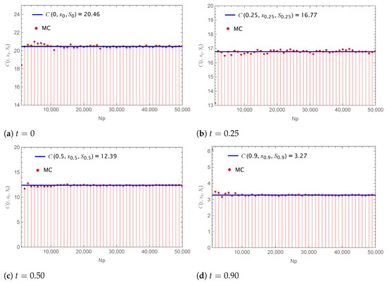
Figure 2. Comparison of the present values of the European call option computed using the explicit Formula (51) with those obtained from Monte Carlo simulations, under the generalized Black-Scholes model, for various initial times $t\in \{0,0.25,0.50,0.95\}$.

Table 1. Comparison of computational time and accuracy in evaluating the call option price at $t=0.5$ using the analytical formulas of the classical and generalized Black-Scholes formulas, together with Monte Carlo simulations.

${\mathit{N}}_{\mathit{p}}$	Error (%)	${\mathit{T}}_{\mathbf{MC}}$ (sec)	${\mathit{T}}_{\mathit{c}}$ (sec)	Reduction (Folds)
Classical Black-Scholes formula at $t=0.5$
$1\times {10}^2$	$0.024$	$0.11$	$0.005$	22
$1\times {10}^3$	$0.019$	$0.98$	$0.005$	196
$1\times {10}^4$	$0.002$	$9.81$	$0.005$	1962
$5\times {10}^4$	$0.002$	$49.44$	$0.005$	9888
Generalized Black-Shole formula at $t=0.5$
$1\times {10}^2$	$0.065$	$0.42$	$0.009$	47
$1\times {10}^3$	$0.011$	$4.25$	$0.009$	472
$1\times {10}^4$	$0.013$	$43.23$	$0.009$	4803
$5\times {10}^4$	$0.007$	$204.70$	$0.009$	$22,744$

Another interesting aspect concerns the difference between the classical and the generalized Black-Scholes option prices. In this experiment, we compute the option value $C(t,S_t)$ under the classical Black-Scholes model using Formula (15), with the same parameter values given in (72) for the GBM process (69), except that the interest rate is taken to be a positive constant

$$r=\sum _{j=1}^3{x}_0^{\left(j\right)}.$$

(74)

Since, in the classical Black-Scholes model, the interest rate appears both in the drift of the GBM (interpreted as the stock’s instantaneous rate of return) and in the discount factor is constant, our goal is to examine how the stochastic evolution of the interest rate affects the option price across different lengths of time to maturity.

Starting from the same initial interest-rate level, Figure 3 shows that the option price under the multifactor Vasicek interest-rate model is consistently lower than the corresponding price under a constant interest rate. Because real-world interest rates—and consequently the rate of return in the stock price dynamics—are not constant, we may conclude that the generalized Black-Scholes model provides a more realistic valuation framework than the classical version.

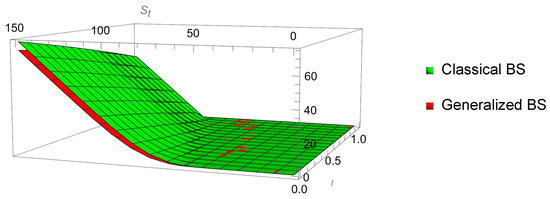
Figure 3. Comparisons of the present values of the European call option under the classical and generalized Black-Scholes models, corresponding to each time to maturity and initial stock price.

6. Conclusions

This study highlights two distinct forms of intersection among three fundamental disciplines—partial differential equations, financial mathematics, and probability—by developing a rigorous analytical framework for the classical Black-Scholes–Merton option pricing model and its generalized extensions. Starting from the stochastic differential representation of the asset dynamics, the pricing problem was reformulated as a well-posed parabolic Cauchy problem equivalent to the classical heat equation. The existence, uniqueness, and stability of classical solutions were established, and explicit pricing formulas were derived via Fourier analysis and Gaussian convolution, providing a solid mathematical justification for European option valuation.

The generalized formulation preserves analytical tractability while allowing a broad class of admissible payoff structures and model extensions. Numerical experiments based on a multifactor Vasicek interest-rate model demonstrated excellent agreement between the closed-form pricing formula and Monte Carlo simulations, together with substantial computational efficiency gains. A comparative analysis further showed that stochastic interest rates yield systematically lower option prices than the classical constant-rate model, highlighting the practical importance of interest-rate dynamics in realistic valuation settings.

Overall, the proposed framework combines mathematical rigor, numerical accuracy, and computational efficiency, offering a robust foundation for further developments in stochastic volatility models, hybrid asset–interest rate dynamics, and high-dimensional derivative pricing.

Possible extension of the current work is to apply this technique to the Black-Scholes PDE for pricing of barrier option, the delta option in Black-Scholes model, or conformable Black-Scholes equation with time-varying parameters [28].

References

- Black, F.; Scholes, M. The pricing of options and corporate liabilities. J. Political Econ. 1973, 81, 637–654. [Google Scholar] [CrossRef]
- Merton, R.C. Theory of Rational Option Pricing; RAND Corporation: Santa Monica, CA, USA, 1971. [Google Scholar]
- Bohner, M.; Zheng, Y. On analytical solutions of the Black-Scholes equation. Appl. Math. Lett. 2009, 22, 309–313. [Google Scholar] [CrossRef]
- Kwan, C.C. Solving the Black-Scholes Partial Differential Equation via the Solution Method for a One-Dimensional Heat Equation: A Pedagogic Approach with a Spreadsheet-Based Illustration. Spreadsheets Educ. 2019, 12, 1–26. [Google Scholar]
- Liu, Y.; Wang, D.S. Symmetry analysis of the option pricing model with dividend yield from financial markets. Appl. Math. Lett. 2011, 24, 481–486. [Google Scholar] [CrossRef][Green Version]
- Saratha, S.; Sai Sundara Krishnan, G.; Bagyalakshmi, M.; Lim, C.P. Solving Black-Scholes equations using fractional generalized homotopy analysis method. Comput. Appl. Math. 2020, 39, 262. [Google Scholar] [CrossRef]
- Jódar, L.; Sevilla-Peris, P.; Cortes, J.; Sala, R. A new direct method for solving the Black-Scholes equation. Appl. Math. Lett. 2005, 18, 29–32. [Google Scholar] [CrossRef]
- Wilmott, P.; Dewynne, J.; Howison, S. Option Pricing: Mathematical Models and Computation; Oxford Financial Press: Oxford, UK, 1993. [Google Scholar]
- Alonso, N.I. Methods for Solving the Black-Scholes Equation; SSRN: Rochester, NY, USA, 2024. [Google Scholar]
- de Souza Santos, D.; Ferreira, T.A. Neural network learning of Black-Scholes equation for option pricing. Neural Comput. Appl. 2025, 37, 2357–2368. [Google Scholar] [CrossRef]
- Yu, B.; Zhu, H.; Wu, P. The closed-form approximation to price basket options under stochastic interest rate. Financ. Res. Lett. 2022, 46, 102434. [Google Scholar] [CrossRef]
- Cox, J.C.; Ingersoll, J.E.; Ross, S.A. A Theory of the Term Structure of Interest Rates. Econometrica 1985, 53, 385–407. [Google Scholar] [CrossRef]
- Chen, R.R.; Scott, L. Pricing interest rate options in a two-factor Cox–Ingersoll–Ross model of the term structure. Rev. Financ. Stud. 1992, 5, 613–636. [Google Scholar] [CrossRef]
- Chen, R.R.; Scott, L. Interest rate options in multifactor cox-ingersoll-ross models of the term structure. J. Deriv. 1995, 3, 53–72. [Google Scholar] [CrossRef]
- Thamrongrat, N.; Chhum, C.; Rujivan, S.; Djehiche, B. An Analytical Formula for the Transition Density of a Conic Combination of Independent Squared Bessel Processes with Time-Dependent Dimensions and Financial Applications. Mathematics 2025, 13, 2106. [Google Scholar] [CrossRef]
- Marek, C.; Tomasz, Z. Mathematics for Finance—An Introduction to Financial Engineering; Springer: Berlin/Heidelberg, Germany, 2016. [Google Scholar]
- Shreve, S.E. Stochastic Calculus for Finance II: Continuous-Time Models; Springer: Berlin/Heidelberg, Germany, 2004; Volume 11. [Google Scholar]
- Hull, J.C.; Basu, S. Options, Futures, and Other Derivatives; Pearson Education India: Delhi, India, 2016. [Google Scholar]
- Salsa, S. Partial Differential Equations in Action; Springer: Berlin/Heidelberg, Germany, 2016. [Google Scholar]
- Stein, E.M.; Shakarchi, R. Fourier Analysis: An Introduction; Princeton University Press: Princeton, NJ, USA, 2011; Volume 1. [Google Scholar]
- Evans, L.C. Partial Differential Equations; American Mathematical Society: Providence, RI, USA, 2022; Volume 19. [Google Scholar]
- Buchanan, J.R. An Undergraduate Introduction to Financial Mathematics; World Scientific: Singapore, 2012. [Google Scholar]
- Friedman, A. Stochastic differential equations and applications. In Stochastic Differential Equations; Springer: Berlin/Heidelberg, Germany, 1975; pp. 75–148. [Google Scholar]
- Brigo, D.; Mercurio, F. Interest Rate Models—Theory and Practice: With Smile, Inflation and Credit; Springer: Berlin/Heidelberg, Germany, 2006. [Google Scholar]
- Privault, N. An Elementary Introduction to Stochastic Interest Rate Modeling; World Scientific: Singapore, 2012; Volume 16. [Google Scholar]
- Björk, T. Arbitrage Theory in Continuous Time; Oxford University Press: Oxford, UK, 2009. [Google Scholar]
- Filipović, D.; Mayerhofer, E. Affine diffusion processes: Theory and. Adv. Financ. Model. 2009, 8, 125. [Google Scholar]
- Morales-Bañuelos, P.; Muriel, N.; Fernández-Anaya, G. A modified Black-Scholes–Merton model for option pricing. Mathematics 2022, 10, 1492. [Google Scholar] [CrossRef]
Disclaimer/Publisher’s Note: The statements, opinions and data contained in all publications are solely those of the individual author(s) and contributor(s) and not of MDPI and/or the editor(s). MDPI and/or the editor(s) disclaim responsibility for any injury to people or property resulting from any ideas, methods, instructions or products referred to in the content. |
© 2026 by the authors. Licensee MDPI, Basel, Switzerland. This article is an open access article distributed under the terms and conditions of the Creative Commons Attribution (CC BY) license.