Dual Physics-Informed Neural Networks Based on Traveling- Wave Decomposition for Boundary Reflection Solutions of Wave Equations

Abstract

We propose a dual physics-informed neural network (Dual-PINN) for wave equations by incorporating the characteristic structure of the one-dimensional d’Alembert solution. Two neural branches are associated with the characteristic coordinates $x-ct$ and $x+ct$ to represent counter-propagating wave components, and their outputs are jointly constrained by the governing equation and auxiliary conditions. Homogeneous Dirichlet boundaries can be imposed exactly through a trial function. For one-dimensional problems, an approximation result shows that the dual-branch representation can approximate solutions of the form $u(x,t)=F(x-ct)+G(x+ct)$ arbitrarily well under standard universal-approximation assumptions, without implying convergence of the non-convex training procedure. Numerical examples involving periodic propagation, boundary reflection, and a two-dimensional wave problem show that the proposed representation captures the tested wave dynamics effectively. The two-dimensional case is treated as an empirical extension, suggesting the potential of characteristic-informed neural representations for wave-equation modeling.

1. Introduction

Wave propagation is a fundamental process in acoustics, elastodynamics, electromagnetics, seismology, and many other areas of science and engineering. Accurate numerical prediction of propagating waves remains challenging because wave fields may exhibit oscillatory structures, reflection and refraction, interference between multiple components, and long-time phase accumulation. These difficulties become particularly pronounced in high-frequency, multidimensional, and heterogeneous-media problems. Conventional discretization-based methods, including finite-difference, finite-element, and spectral-type schemes, remain powerful tools for wave simulations. However, accurate long-time or high-frequency simulations often require sufficiently fine spatial and temporal resolutions to control dispersion and stability errors, which can substantially increase the computational cost, especially for multidimensional problems [1,2,3,4,5,6,7,8,9,10,11,12].

Physics-informed neural networks (PINNs) provide a mesh-free framework for solving forward and inverse problems of partial differential equations (PDEs) by incorporating the governing equations together with available initial, boundary, or observational data into the training objective [13,14]. Unlike purely data-driven surrogate models, PINNs can exploit physical constraints and therefore reduce their dependence on labeled solution data. Nevertheless, the approximation capability of a neural network does not necessarily translate into an easily trainable physics-informed model. Previous studies have shown that PINNs may suffer from imbalanced gradients among different loss components, poorly conditioned optimization landscapes, and disparate convergence behaviors associated with different physical constraints [15,16,17,18]. Adaptive activation functions [19,20] and related optimization strategies have therefore been developed to improve trainability and representation accuracy. Such difficulties are particularly relevant to wave equations, where oscillatory, propagating, and multiscale structures impose additional requirements on both neural representation and optimization.

A number of studies have improved PINNs for wave propagation from the perspectives of optimization, activation design, and constraint enforcement. Moseley et al. [9] applied PINNs to two-dimensional acoustic-wave propagation in homogeneous, layered, and geologically complex velocity models, demonstrating the feasibility of physics-informed learning for propagating wave fields. Rasht-Behesht et al. [10] further investigated acoustic-wave forward modeling and full-waveform inversion. For the one-dimensional wave equation, Nosrati and Emami Niri [21] analyzed the influence of the multi-term PINN loss and modified its calculation to improve training, whereas Alkhadhr and Almekkawy [22] introduced adaptive attention to the loss weights for acoustic-wave modeling. Maczuga and Paszyński [23] systematically examined the effects of activation functions and different treatments of initial and boundary conditions on PINN convergence. In addition, Alkhadhr and Almekkawy [24] compared soft and hard enforcement of initial and boundary conditions for wave-equation modeling. These studies demonstrate that loss balancing, activation design, and constraint enforcement can substantially influence the performance of wave PINNs. However, the wave field is still generally represented as a single neural mapping of the original space–time coordinates.

Another important direction is to incorporate analytical or structural information from the underlying wave problem into the learning process. Lin et al. [25] introduced conservation laws into a two-stage PINN for localized-wave solutions of integrable nonlinear equations, illustrating the benefit of embedding additional mathematical structure into physics-informed learning. For high-frequency wave-field representation, Song and Wang [26] employed Fourier-feature embeddings to alleviate the spectral bias of PINNs in multifrequency seismic-wave simulations. Wu et al. [27] developed IS-PINN for inhomogeneous wave equations by incorporating separation of variables, the superposition principle, and Duhamel’s principle into the solution framework. Liu et al. [28] combined linear wave theory with PINNs for phase-resolved wave prediction, while Qi and Sarris [29] coupled neural-network spatial differentiation with an unconditionally stable time-stepping strategy for electromagnetic wave simulations. Multi-network formulations have also been investigated from other perspectives. For example, XPINNs employ multiple subnetworks associated with different space–time subdomains [30]. Hard enforcement of boundary conditions through specially constructed trial functions has also been investigated in the broader PINN literature [31]. Van der Meer et al. optimized global weights across loss terms, while McClenny and Braga-Neto introduced adaptive weighting at individual training points, both mitigating loss imbalance during PINN training and improving solution accuracy [32,33].

Despite these developments, existing approaches mainly improve loss weighting, optimization, feature representation, boundary enforcement, temporal integration, or decomposition of the computational domain. For the one-dimensional homogeneous linear wave equation, however, the d’Alembert solution reveals a more specific directional structure,

$$u(x,t)=F(x-ct)+G(x+ct),$$

(1)

where $F(x-ct)$ and $G(x+ct)$ represent two counter-propagating characteristic components. This structure is fundamentally different from decomposing the computational domain or enriching the original space–time input. When the characteristic directions are not explicitly represented, a conventional PINN must learn the propagation directions, phase evolution, and interaction of incident and reflected components simultaneously through a single mapping from $(x,t)$ to $u(x,t)$. This issue is particularly relevant to boundary-reflection problems, in which counter-propagating components coexist and interact over time.

Motivated by this analytical structure, we develop a Dual Physics-Informed Neural Network (Dual-PINN) in which two neural branches are explicitly associated with the characteristic coordinates $x-ct$ and $x+ct$. Their outputs are combined to construct the wave-field approximation and are jointly constrained by the governing equation and the prescribed initial and boundary conditions. The contribution of the present work is therefore not the use of multiple neural networks itself, but the direct architectural correspondence between the two neural branches and the two characteristic propagation directions of the one-dimensional linear wave equation. For homogeneous Dirichlet reflection problems, a problem-specific trial function is additionally introduced to enforce the boundary conditions exactly. The approximation property of the characteristic dual-branch representation is analyzed in the one-dimensional setting, and the proposed framework is evaluated on a periodic-wave benchmark and a boundary-reflection problem. A two-dimensional wave problem is further considered as an empirical extension to examine the applicability of the dual-network framework beyond the exact one-dimensional d’Alembert representation.

2. Problem Formulation

Let $\mathrm{\Omega }\subset {\mathbb{R}}^d$ be a bounded spatial domain, where d denotes the spatial dimension. We consider the following linear wave problem:

$$\left\{\begin{array}{cc}{u}_{tt}(\mathbf{x},t)-c^2\mathrm{\Delta }u(\mathbf{x},t)=f(\mathbf{x},t),\hfill & (\mathbf{x},t)\in \mathrm{\Omega }\times (0,t_f],\hfill \\ u(\mathbf{x},0)=\varphi \left(\mathbf{x}\right),\hfill & \mathbf{x}\in \mathrm{\Omega },\hfill \\ u_t(\mathbf{x},0)=\psi \left(\mathbf{x}\right),\hfill & \mathbf{x}\in \mathrm{\Omega },\hfill \\ u(\mathbf{x},t)=g(\mathbf{x},t),\hfill & (\mathbf{x},t)\in \partial \mathrm{\Omega }\times (0,t_f].\hfill \end{array}\right.$$

(2)

Here, $u(\mathbf{x},t)$ denotes the wave field, $c>0$ is the wave propagation speed, $f(\mathbf{x},t)$ is a prescribed source term, $\varphi \left(\mathbf{x}\right)$ and $\psi \left(\mathbf{x}\right)$ denote the prescribed initial displacement and initial velocity, respectively, and $g(\mathbf{x},t)$ specifies the Dirichlet boundary data.

For convenience, define the linear differential operator

$${\mathcal{L}}_c\left[u\right](\mathbf{x},t):=u_{tt}(\mathbf{x},t)-c^2\mathrm{\Delta }u(\mathbf{x},t).$$

(3)

Because ${\mathcal{L}}_c$ is linear, the corresponding wave problem satisfies the superposition principle. Specifically, if $u_1$ and $u_2$ are solutions associated with the data $(f_1,{\varphi }_1,{\psi }_1,g_1)$ and $(f_2,{\varphi }_2,{\psi }_2,g_2)$, respectively, then, for any constants $\alpha$ and $\beta$, the function $\alpha u_1+\beta u_2$ is associated with the combined data

$$(\alpha f_1+\beta f_2,\alpha {\varphi }_1+\beta {\varphi }_2,\alpha {\psi }_1+\beta {\psi }_2,\alpha g_1+\beta g_2).$$

To motivate the traveling-wave representation used in this work, we first consider the homogeneous one-dimensional wave equation on the real line:

$$\left\{\begin{array}{cc}{u}_{tt}(x,t)=c^2{u}_{xx}(x,t),\hfill & (x,t)\in \mathbb{R}\times (0,t_f],\hfill \\ u(x,0)=\varphi \left(x\right),\hfill & x\in \mathbb{R},\hfill \\ u_t(x,0)=\psi \left(x\right),\hfill & x\in \mathbb{R}.\hfill \end{array}\right.$$

(4)

Introducing the characteristic coordinates

$$\xi =x-ct,\eta =x+ct,$$

(5)

the solution can be represented as the superposition of two counter-propagating traveling-wave components,

$$u(x,t)=F\left(\xi \right)+G\left(\eta \right)=F(x-ct)+G(x+ct),$$

(6)

where $F(x-ct)$ represents a right-going wave and $G(x+ct)$ represents a left-going wave, both propagating with speed c.

For the prescribed initial conditions in Equation (4), the corresponding d’Alembert formula is

$$u(x,t)={\displaystyle \frac{1}{2}}\left[\varphi (x-ct)+\varphi (x+ct)\right]+{\displaystyle \frac{1}{2c}}{\int }_{x-ct}^{x+ct}\psi \left(s\right)ds.$$

(7)

Equivalently, for an arbitrary reference point $x_0$, the two characteristic components can be written as

$$F\left(\xi \right)={\displaystyle \frac{1}{2}}\varphi \left(\xi \right)-{\displaystyle \frac{1}{2c}}{\int }_{x_0}^{\xi }\psi \left(s\right)ds,$$

(8)

and

$$G\left(\eta \right)={\displaystyle \frac{1}{2}}\varphi \left(\eta \right)+{\displaystyle \frac{1}{2c}}{\int }_{x_0}^{\eta }\psi \left(s\right)ds.$$

(9)

It should be emphasized that the classical d’Alembert representation above is stated for the wave equation on the real line. On a bounded interval, the boundary conditions impose additional compatibility relations between the two characteristic components.

For example, consider $\mathrm{\Omega }=(0,L)$ with homogeneous Dirichlet boundary conditions,

$$u(0,t)=u(L,t)=0.$$

(10)

If

$$u(x,t)=F(x-ct)+G(x+ct),$$

(11)

then the boundary conditions require

$$F(-ct)+G\left(ct\right)=0,$$

(12)

and

$$F(L-ct)+G(L+ct)=0.$$

(13)

Therefore, the right-going and left-going components are not independent on a bounded interval; they are coupled through the prescribed boundary conditions and the associated reflection process.

In the proposed Dual-PINN, this coupling is incorporated through the physics-informed constraints imposed on the combined output of the two neural branches. Thus, the characteristic decomposition is used to define the directional structure of the neural representation rather than to assume that the two traveling-wave components remain unconstrained on a bounded domain.

Neural Network Representation for the Wave Equation

To approximate the solution of the wave problem in Equation (2). Let

$${\mathcal{N}}_{\mathrm{\Theta }}:{\mathbb{R}}^{D_i}\to \mathbb{R}$$

denote a fully connected feed-forward neural network, where $\mathrm{\Theta }$ denotes the collection of trainable parameters.

For a standard space–time representation, the input vector is denoted by $\mathbf{z}\in {\mathbb{R}}^{D_i}$. For the scalar wave problems considered in this work, the network output is one-dimensional, i.e., $D_o=1$.

For a conventional space–time PINN, the input can be written as

$$\mathbf{z}=(\mathbf{x},t),$$

whereas the characteristic branches introduced in Section 3 use problem-specific transformed inputs.

Let the network contain $L_h$ hidden layers, with $N_k$ neurons in the kth hidden layer. The weight matrix and bias vector associated with the kth layer are denoted by ${\mathbf{W}}^{\left(k\right)}$ and ${\mathbf{b}}^{\left(k\right)}$, respectively. We define the input layer as

$${\mathbf{h}}^{\left(0\right)}=\mathbf{z}.$$

(14)

Following [19,20], locally adaptive activation functions are employed in the hidden layers. Let $\sigma (·)$ denote the activation function, $n>0$ be a prescribed scaling factor, and $a_k$ be the trainable activation-slope parameter associated with the kth hidden layer. The hidden-layer transformation is defined as

$${\mathbf{h}}^{\left(k\right)}=\sigma \left(n{a}_k\left[{\mathbf{W}}^{\left(k\right)}{\mathbf{h}}^{(k-1)}+{\mathbf{b}}^{\left(k\right)}\right]\right),k=1,\dots ,L_h.$$

(15)

Here, $a_k$ is optimized together with the network weights and biases, allowing the effective slope of the activation function to adapt during training. Such locally adaptive activation functions have been shown to improve the trainability of deep and physics-informed neural networks [19,20]. Let $N_0=D_i$. For $k=1,\dots ,L_h$,

$${\mathbf{W}}^{\left(k\right)}\in {\mathbb{R}}^{N_k\times N_{k-1}},{\mathbf{b}}^{\left(k\right)}\in {\mathbb{R}}^{N_k}.$$

The output layer is taken to be linear and is written as

$${\mathcal{N}}_{\mathrm{\Theta }}\left(\mathbf{z}\right)={\mathbf{W}}^{(L_h+1)}{\mathbf{h}}^{\left(L_h\right)}+{\mathbf{b}}^{(L_h+1)}.$$

(16)

Accordingly, the complete set of trainable parameters is

$$\mathrm{\Theta }={\left\{{\mathbf{W}}^{\left(k\right)},{\mathbf{b}}^{\left(k\right)}\right\}}_{k=1}^{L_h+1}\cup {\left\{a_k\right\}}_{k=1}^{L_h}.$$

(17)

In the numerical experiments, the scaling factor is fixed at $n=5$. The initialization of the adaptive slope parameters $a_k$ is kept identical for all hidden layers and is specified together with the remaining training settings in the numerical section.

3. Dual Physics-Informed Neural Networks Based on Traveling-Wave Decomposition

The standard PINN framework approximates the solution of a governing partial differential equation using a neural network and incorporates the governing equation, initial conditions, boundary conditions, and, when available, labeled observations into a unified loss function. For wave problems, however, a single space–time mapping does not explicitly exploit the directional structure revealed by the characteristic representation of the one-dimensional wave equation.

As shown in Section 2, the solution of the one-dimensional homogeneous linear wave equation can be represented as

$$u(x,t)=F(x-ct)+G(x+ct),$$

(18)

where $F(x-ct)$ and $G(x+ct)$ represent right-going and left-going traveling-wave components, respectively. This analytical structure motivates the proposed dual-branch neural representation.

3.1. Characteristic Dual-Branch Representation

Introducing the characteristic coordinates

$$\xi =x-ct,\eta =x+ct,$$

(19)

we employ two independent feed-forward neural networks to approximate the two counter-propagating components:

$${\widehat{u}}_{+}(x,t)={\mathcal{N}}_{+}(\xi ;{\theta }_{+})={\mathcal{N}}_{+}(x-ct;{\theta }_{+}),$$

(20)

and

$${\widehat{u}}_{-}(x,t)={\mathcal{N}}_{-}(\eta ;{\theta }_{-})={\mathcal{N}}_{-}(x+ct;{\theta }_{-}),$$

(21)

where ${\theta }_{+}$ and ${\theta }_{-}$ denote the trainable parameters of the right-going and left-going branches, respectively.

The Dual-PINN approximation is then defined as

$$\widehat{u}(x,t;\mathrm{\Theta })={\widehat{u}}_{+}(x,t)+{\widehat{u}}_{-}(x,t)={\mathcal{N}}_{+}(x-ct;{\theta }_{+})+{\mathcal{N}}_{-}(x+ct;{\theta }_{-}),$$

(22)

where ${\theta }_{+}$ and ${\theta }_{-}$ denote the parameter sets of the two branches and

$$\mathrm{\Theta }={\theta }_{+}\cup {\theta }_{-}.$$

Although the two branches have separate parameter sets, they are optimized jointly through the constraints imposed on their combined output. In particular, the initial and boundary conditions couple the two characteristic components and thereby determine their interaction in bounded-domain reflection problems.

An important property of Equation (22) is that each branch satisfies the one-dimensional homogeneous wave operator identically. Indeed,

$${\partial }_{tt}{\mathcal{N}}_{+}(x-ct)-c^2{\partial }_{xx}{\mathcal{N}}_{+}(x-ct)=0,$$

(23)

and similarly,

$${\partial }_{tt}{\mathcal{N}}_{-}(x+ct)-c^2{\partial }_{xx}{\mathcal{N}}_{-}(x+ct)=0.$$

(24)

Consequently,

$${\widehat{u}}_{tt}-c^2{\widehat{u}}_{xx}=0$$

(25)

for the raw characteristic representation in Equation (22). Thus, for the homogeneous one-dimensional problem, the governing equation is encoded directly into the functional form of the two branches, while the initial and boundary conditions determine the admissible combination of the two components.

For homogeneous Dirichlet problems, a problem-specific trial factor $B\left(x\right)$ may additionally be introduced:

$$\widehat{u}(x,t;\mathrm{\Theta })=B\left(x\right)\left[{\mathcal{N}}_{+}(x-ct;{\theta }_{+})+{\mathcal{N}}_{-}(x+ct;{\theta }_{-})\right],$$

(26)

where $B\left(x\right)=0$ on the spatial boundary. Because multiplication by $B\left(x\right)$ modifies the exact d’Alembert form, the resulting trial solution does not satisfy the wave operator identically; in this case, the PDE residual is retained as a training constraint.

The characteristic interpretation above is specific to the one-dimensional linear wave equation with constant wave speed. The two-dimensional formulation considered later is treated as an empirical dual-network extension and is not interpreted as a direct d’Alembert decomposition.

3.2. Physics-Informed Loss Function

For the general wave problem defined in Equation (2), let

$${\mathcal{S}}_r={\left\{({\mathbf{x}}_i^r,t_i^r)\right\}}_{i=1}^{N_r}\subset \mathrm{\Omega }\times (0,t_f]$$

(27)

denote the set of interior collocation points,

$${\mathcal{S}}_0={\left\{{\mathbf{x}}_i^0\right\}}_{i=1}^{N_0}\subset \mathrm{\Omega }$$

(28)

the set of initial-condition points, and

$${\mathcal{S}}_b={\left\{({\mathbf{x}}_i^b,t_i^b)\right\}}_{i=1}^{N_b}\subset \partial \mathrm{\Omega }\times (0,t_f]$$

(29)

the set of boundary points. Here, $N_r$, $N_0$, $N_b$, and $N_d$ denote the numbers of interior residual points, initial-condition points, boundary-condition points, and labeled data points, respectively.

For the neural approximation $\widehat{u}(\mathbf{x},t;\mathrm{\Theta })$, the PDE residual is defined as

$$\mathcal{R}(\mathbf{x},t;\mathrm{\Theta })={\partial }_{tt}\widehat{u}(\mathbf{x},t;\mathrm{\Theta })-c^2\mathrm{\Delta }\widehat{u}(\mathbf{x},t;\mathrm{\Theta })-f(\mathbf{x},t).$$

(30)

The corresponding residual loss is

$${\mathcal{L}}_r={\displaystyle \frac{1}{N_r}}{\displaystyle \sum _{i=1}^{N_r}}{\left|\mathcal{R}({\mathbf{x}}_i^r,t_i^r;\mathrm{\Theta })\right|}^2.$$

(31)

The initial-condition loss accounts for both the prescribed displacement and velocity and is defined as

$$\begin{array}{cc}\hfill {\mathcal{L}}_0=& {\displaystyle \frac{1}{N_0}}{\displaystyle \sum _{i=1}^{N_0}}{\left|\widehat{u}({\mathbf{x}}_i^0,0;\mathrm{\Theta })-\varphi \left({\mathbf{x}}_i^0\right)\right|}^2\hfill \\ \hfill & +{\displaystyle \frac{1}{N_0}}{\displaystyle \sum _{i=1}^{N_0}}{\left|{\partial }_t\widehat{u}({\mathbf{x}}_i^0,0;\mathrm{\Theta })-\psi \left({\mathbf{x}}_i^0\right)\right|}^2,\hfill \end{array}$$

(32)

Both terms are normalized by the same number of samples so that no unintended imbalance is introduced between the displacement and velocity constraints.

For the Dirichlet boundary condition defined in Equation (2), the boundary loss is

$${\mathcal{L}}_b={\displaystyle \frac{1}{N_b}}{\displaystyle \sum _{i=1}^{N_b}}{\left|\widehat{u}({\mathbf{x}}_i^b,t_i^b;\mathrm{\Theta })-g({\mathbf{x}}_i^b,t_i^b)\right|}^2.$$

(33)

When labeled observations are available, we denote the corresponding data set by

$${\mathcal{S}}_d={\left\{({\mathbf{x}}_i^d,t_i^d,y_i^d)\right\}}_{i=1}^{N_d},$$

(34)

and define the data loss as

$${\mathcal{L}}_d={\displaystyle \frac{1}{N_d}}{\displaystyle \sum _{i=1}^{N_d}}{\left|\widehat{u}({\mathbf{x}}_i^d,t_i^d;\mathrm{\Theta })-y_i^d\right|}^2.$$

(35)

The total physics-informed loss is therefore written consistently as

$$\mathcal{L}\left(\mathrm{\Theta }\right)={\omega }_r{\mathcal{L}}_r+{\omega }_0{\mathcal{L}}_0+{\omega }_b{\mathcal{L}}_b+{\omega }_d{\mathcal{L}}_d,$$

(36)

where ${\omega }_r$, ${\omega }_0$, ${\omega }_b$, and ${\omega }_d$ are nonnegative weights associated with the PDE residual, initial conditions, boundary conditions, and labeled data, respectively. When no labeled data are used, the last term is omitted (or equivalently ${\omega }_d=0$).

For examples in which the Dirichlet boundary condition is imposed exactly through a specifically constructed trial function, the corresponding boundary-loss term can be omitted. Such hard enforcement is described separately for the relevant numerical examples.

3.3. Optimization

The trainable parameters of the Dual-PINN are determined by minimizing the total loss:

$${\mathrm{\Theta }}^{\ast }=\arg \underset{\mathrm{\Theta }}{\min }\mathcal{L}\left(\mathrm{\Theta }\right).$$

(37)

The spatial and temporal derivatives appearing in Equation (30) are evaluated by automatic differentiation.

It is important to distinguish the well-posedness of the underlying wave equation from the optimization of the neural network. Well-posedness concerns the existence, uniqueness, and continuous dependence of the PDE solution on the prescribed data, but does not guarantee convergence to a global minimizer of the non-convex optimization problem in Equation (37). Therefore, no optimizer-specific global-convergence claim is made here. The optimization algorithms and their corresponding settings used in the numerical experiments, including Adam and L-BFGS where applicable, are reported explicitly in the numerical section.

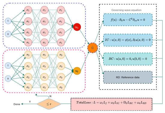
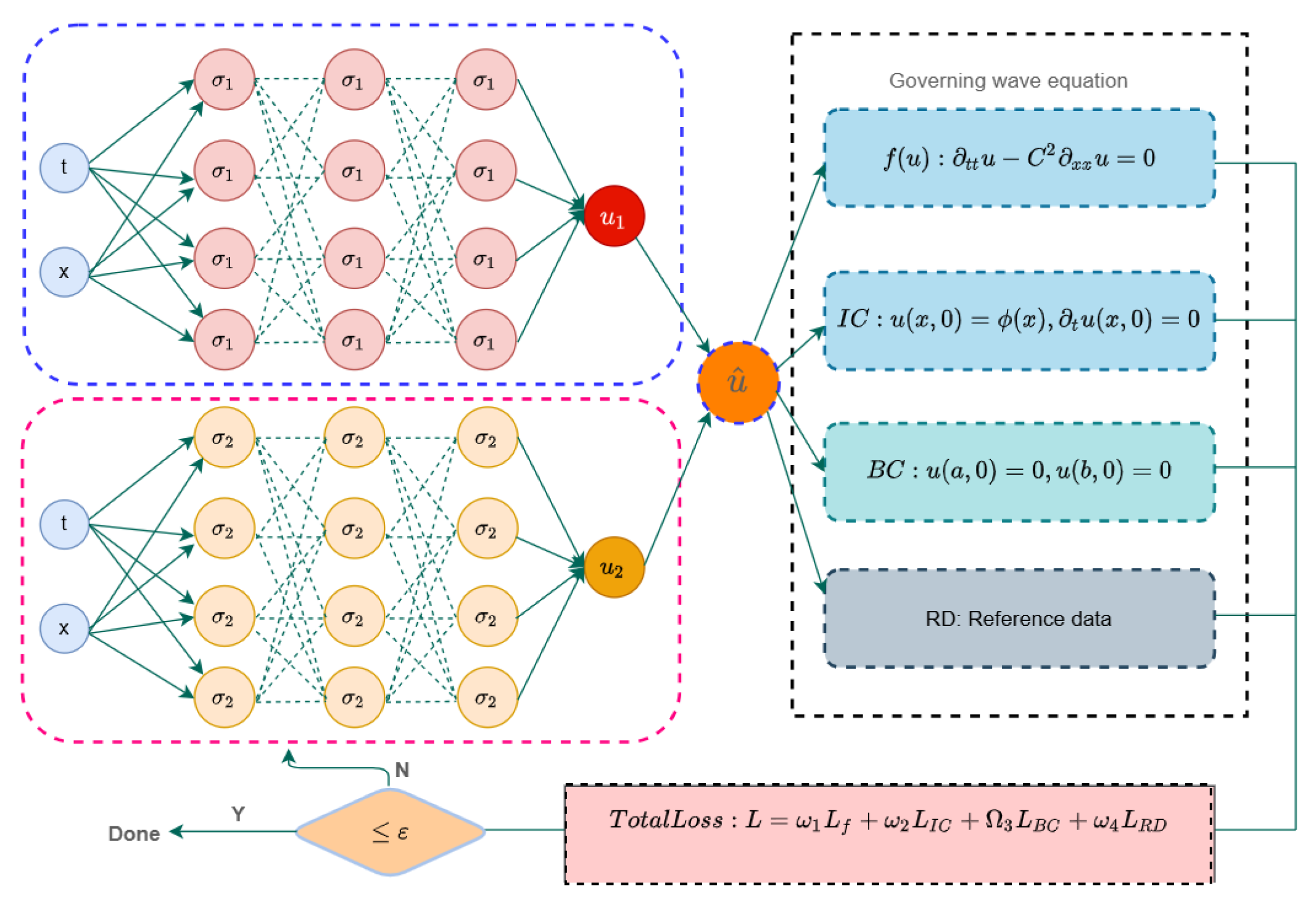
We construct a dual-network architecture, as illustrated in Figure 1, to approximate the solution of the wave equation. The two neural branches are designed to represent the two counter-propagating components associated with the characteristic coordinates $x-ct$ and $x+ct$, respectively.

Figure 1. Schematic of the proposed Dual-PINN for the one-dimensional wave equation. The two neural branches take the characteristic coordinates $\xi =x-ct$ and $\eta =x+ct$ as inputs to represent the right-going and left-going wave components, respectively. Their outputs are combined to form the prediction $\widehat{u}(x,t)$, which is jointly constrained by the governing equation and the initial and boundary conditions.

4. Approximation Properties of the One-Dimensional Characteristic Dual-Branch Representation

The purpose of this section is to analyze the representational approximation capability of the characteristic dual-branch architecture introduced in Section 3. The analysis addresses whether suitable neural-network parameters exist such that the two characteristic components can be approximated to arbitrary accuracy. It should be distinguished from both the minimization of the discrete physics-informed loss and the convergence of the numerical optimization procedure used during training.

4.1. Scope and Assumptions

Consider the one-dimensional homogeneous linear wave equation

$$u_{tt}(x,t)=c^2{u}_{xx}(x,t),(x,t)\in Q,$$

(38)

where

$$Q=\mathrm{\Omega }\times [0,t_f],\mathrm{\Omega }=(x_L,x_R),$$

(39)

and $c>0$ is the constant wave propagation speed.

As discussed in Section 2, suppose that the exact solution admits the characteristic representation

$$u(x,t)=F(x-ct)+G(x+ct),$$

(40)

where F and G denote the right-going and left-going characteristic components, respectively.

For $(x,t)\in Q$, the corresponding characteristic variables satisfy

$$x-ct\in I_{+},x+ct\in I_{-},$$

where

$$I_{+}=[x_L-c{t}_f,x_R],I_{-}=[x_L,x_R+c{t}_f].$$

(41)

We assume that

$$F\in C\left(I_{+}\right),G\in C\left(I_{-}\right).$$

(42)

The characteristic representation in Equation (40) is specific to the one-dimensional linear wave equation under the corresponding assumptions. Therefore, the theoretical result below is restricted to the one-dimensional setting and is not intended as a representation theorem for general two-dimensional wave equations.

4.2. Approximation Property

Consistent with the Dual-PINN formulation in Section 3, we consider the neural representation

$$\widehat{u}(x,t;\mathrm{\Theta })={\mathcal{N}}_{+}(x-ct;{\theta }_{+})+{\mathcal{N}}_{-}(x+ct;{\theta }_{-}),$$

(43)

where ${\mathcal{N}}_{+}$ and ${\mathcal{N}}_{-}$ are two independent feed-forward neural networks and

$$\mathrm{\Theta }=\{{\theta }_{+},{\theta }_{-}\}.$$

(44)

Proposition 1

(Approximation Property of the Characteristic Dual-Branch Representation). Assume that the exact solution u satisfies Equation (40), with $F\in C\left(I_{+}\right)$ and $G\in C\left(I_{-}\right)$. For any $\epsilon >0$, there exist two feed-forward neural networks ${\mathcal{N}}_{+}$ and ${\mathcal{N}}_{-}$, with activation functions satisfying the standard conditions of the universal approximation theorem, such that

$${∥u-\widehat{u}∥}_{L^{\infty }\left(Q\right)}<\epsilon .$$

(45)

Proof. 

Since F is continuous on the compact interval $I_{+}$, the universal approximation theorem implies that, for any $\epsilon >0$, there exists a feed-forward neural network ${\mathcal{N}}_{+}$ satisfying

$$\underset{\xi \in I_{+}}{\sup }\left|F\left(\xi \right)-{\mathcal{N}}_{+}(\xi ;{\theta }_{+})\right|<{\displaystyle \frac{\epsilon }{2}}.$$

(46)

Similarly, because $G\in C\left(I_{-}\right)$, there exists a feed-forward neural network ${\mathcal{N}}_{-}$ such that

$$\underset{\eta \in I_{-}}{\sup }\left|G\left(\eta \right)-{\mathcal{N}}_{-}(\eta ;{\theta }_{-})\right|<{\displaystyle \frac{\epsilon }{2}}.$$

(47)

For any $(x,t)\in Q$, Equations (40) and (43) give

$$\begin{array}{cc}\hfill \left|u(x,t)-\widehat{u}(x,t;\mathrm{\Theta })\right|& =|F(x-ct)-{\mathcal{N}}_{+}(x-ct;{\theta }_{+})\hfill \\ \hfill & +G(x+ct)-{\mathcal{N}}_{-}(x+ct;{\theta }_{-})|\hfill \\ \hfill & \le \left|F(x-ct)-{\mathcal{N}}_{+}(x-ct;{\theta }_{+})\right|\hfill \\ \hfill & +\left|G(x+ct)-{\mathcal{N}}_{-}(x+ct;{\theta }_{-})\right|\hfill \\ \hfill & <\epsilon .\hfill \end{array}$$

(48)

Taking the supremum over Q proves Equation (45). □

Since Q has finite measure, Equation (45) also implies

$${∥u-\widehat{u}∥}_{L^2\left(Q\right)}\le {\left|Q\right|}^{1/2}{∥u-\widehat{u}∥}_{L^{\infty }\left(Q\right)}.$$

(49)

Thus, the dual-branch representation can also achieve arbitrarily small $L^2$ approximation error under the same assumptions.

4.3. Interpretation and Limitations

Proposition 1 establishes an approximation property of the characteristic dual-branch representation. It shows that, when the exact solution admits the decomposition $u(x,t)=F(x-ct)+G(x+ct)$, the two neural branches can approximate the corresponding characteristic components independently and their outputs can be combined to approximate the full solution.

This result concerns representational capability only. It does not imply that gradient-based optimization will necessarily identify the corresponding network parameters, and it does not establish convergence of the non-convex training procedure.

Proposition 1 also does not establish that the Dual-PINN has a higher approximation order than a conventional PINN. The potential practical benefit of the characteristic decomposition is instead evaluated empirically in Section 5 through matched comparisons of prediction accuracy and training behavior.

Finally, the exact characteristic decomposition used in Proposition 1 is specific to the one-dimensional linear wave equation. The two-dimensional case considered in the numerical experiments is treated as an empirical extension of the dual-network framework and is not covered by the above proposition.

5. Experiments and Result Analysis

We consider three numerical examples to evaluate the performance of the proposed Dual-PINN. The relative $L_2$ error and maximum absolute error are defined as

$$E_{\mathrm{rel},2}={\displaystyle \frac{{\left({\sum }_{j=1}^{N_t}{|{\widehat{u}}_j-u_j^{\mathrm{ref}}|}^2\right)}^{1/2}}{{\left({\sum }_{j=1}^{N_t}{\left|u_j^{\mathrm{ref}}\right|}^2\right)}^{1/2}}},E_{\infty }=\underset{1\le j\le N_t}{\max }|{\widehat{u}}_j-u_j^{\mathrm{ref}}|,$$

(50)

respectively.

For a fair comparison, the PINN and Dual-PINN are constructed using the same total number of hidden neurons. The conventional PINN consists of a single network with four hidden layers and 20 neurons per layer, whereas the Dual-PINN contains two independent branches, each consisting of two hidden layers with 20 neurons per layer. Therefore, both architectures contain a total of 80 hidden neurons. The detailed network hyperparameter and hardware configurations of the standard PINN and the proposed Dual-PINN for 1D wave equation benchmark are summarized in Table 1.

Table 1. Network configurations used for the one-dimensional comparison between the PINN and Dual-PINN.

Configuration	PINN	Dual-PINN
Number of networks	1	2
Hidden layers	4	2 per branch
Neurons per hidden layer	20	20 per branch
Total hidden neurons	80	80
Trainable parameters	1341	962
Activation function	sine
Optimizer	L-BFGS
Learning Rate	0.005
Maximum iterations	1000 (1D); 3000 (2D)
Hardware information	Intel i7-13700H, NVIDIA RTX4060, 32 GB RAM

All other training settings are kept identical for the two methods. Both models use the sine activation function and are optimized using L-BFGS. Furthermore, the same collocation points, initial and boundary samples, loss weights, numerical precision, stopping criterion, and computational hardware are used. Thus, the comparison is designed to isolate the effect of the proposed dual-branch decomposition rather than differences in training configuration.

5.1. Example 1: Periodic One-Dimensional Wave Equation

We first consider

$$u_{tt}-4u_{xx}=0,(x,t)\in [0,1]\times [0,1],$$

(51)

subject to homogeneous Dirichlet boundary conditions. The analytical solution is

$$u(x,t)=\sin \left(\pi x\right)\cos \left(2\pi t\right)+{\displaystyle \frac{1}{2}}\sin \left(4\pi x\right)\cos \left(8\pi t\right),$$

(52)

from which the initial conditions are obtained. A total of 3000 interior collocation points and 500 initial points are used.

5.2. Sensitivity to Network Architecture

We investigate the sensitivity of the Dual-PINN to network depth and width using Example 1.

Table 2 shows a non-monotonic dependence of the prediction accuracy on network depth and width. Increasing the network size does not consistently reduce the error, while the computational cost increases steadily. Among the tested configurations, the $2\times 20$ architecture achieves the smallest relative $L_2$ error of $1.19\times {10}^{-3}$, with a training time of $49.9\mathrm{s}$. It is therefore adopted for the subsequent one-dimensional experiments as a favorable accuracy–cost compromise.

Table 2. Sensitivity of the Dual-PINN to network depth and width for Example 1.

${\mathit{L}}_{\mathit{h}}$	${\mathit{N}}_{\mathit{h}}$	${\mathit{E}}_{\mathbf{rel},2}$	${\mathit{E}}_{\mathit{\infty }}$	Time (s)
2	10	5.08 × 10−3	1.56 × 10−2	38.6
2	20	1.19 × 10−3	2.36 × 10−3	49.9
2	40	1.28 × 10−3	2.92 × 10−3	59.9
3	10	2.96 × 10−3	7.27 × 10−3	56.8
3	20	1.71 × 10−3	4.36 × 10−3	75.1
3	40	1.40 × 10−3	4.07 × 10−3	92.8
4	10	2.90 × 10−3	7.17 × 10−3	71.6
4	20	1.45 × 10−3	4.46 × 10−3	96.3
4	40	1.62 × 10−3	3.51 × 10−3	122.5

For the matched comparison between the conventional PINN and Dual-PINN in Example 1, the experiments are repeated using five independent random initializations, and the corresponding results are reported as mean ± standard deviation. Unless otherwise stated, the remaining numerical examples are reported from individual runs and are intended to illustrate the numerical behavior of the proposed formulation rather than to provide a statistical robustness assessment across all test problems.

Table 3 shows that the Dual-PINN consistently achieves lower errors than the conventional PINN over five independent runs. In particular, the final loss decreases from $1.1\times {10}^{-3}$ to $3.3\times {10}^{-6}$, while the relative $L_2$ error and maximum error are reduced from $4.5\times {10}^{-2}$ and $5.9\times {10}^{-1}$ to $1.7\times {10}^{-3}$ and $8.8\times {10}^{-3}$, respectively. Meanwhile, the average training time is slightly lower for the Dual-PINN, indicating that the improved accuracy is achieved without additional computational cost.

Table 3. Comparison of PINN and Dual-PINN over five independent runs for Example 1. Results are reported as mean ± standard deviation.

Method	Final Loss	${\mathit{E}}_{\mathbf{rel},2}$	${\mathit{E}}_{\mathit{\infty }}$	Training Time (s)
PINN	$1.1\times {10}^{-3}\pm 4.3\times {10}^{-4}$	$4.5\times {10}^{-2}\pm 8.2\times {10}^{-3}$	$5.9\times {10}^{-1}\pm 3.3\times {10}^{-2}$	$96.5\pm 5.8$
Dual-PINN	$3.3\times {10}^{-6}\pm 3.4\times {10}^{-7}$	$1.7\times {10}^{-3}\pm 7.6\times {10}^{-4}$	$8.8\times {10}^{-3}\pm 1.2\times {10}^{-4}$	$88.8\pm 5.5$

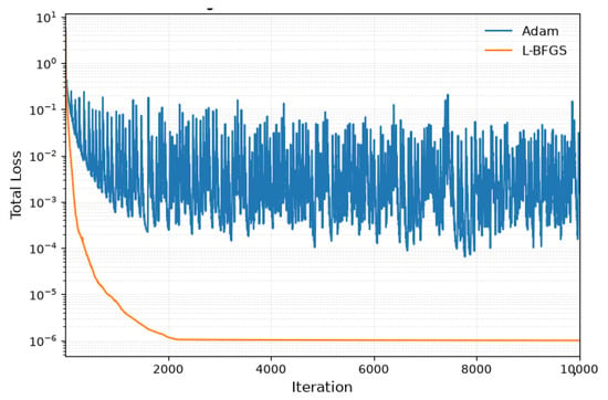
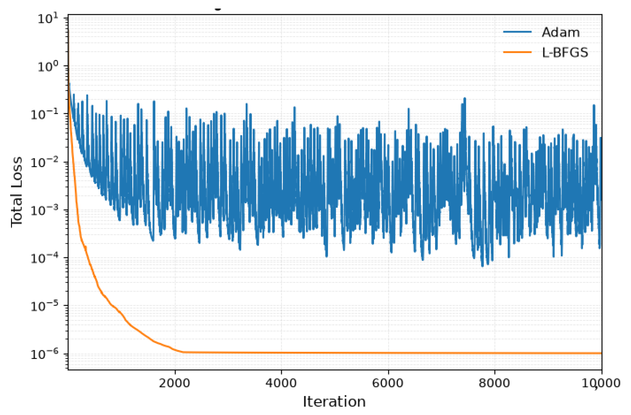
Figure 2 compares the loss convergence of the Dual-PINN trained with Adam and L-BFGS. Adam reduces the loss rapidly at the early stage but exhibits persistent oscillations during subsequent iterations, with the loss remaining within approximately ${10}^{-4}$–${10}^{-2}$. In contrast, L-BFGS shows a smoother convergence behavior and decreases the loss to approximately ${10}^{-5}$ after about 1000 iterations. These results indicate that L-BFGS provides more stable late-stage convergence and a lower final training loss for the present problem.

Figure 2. Loss convergence of Dual-PINN with Adam and L-BFGS.

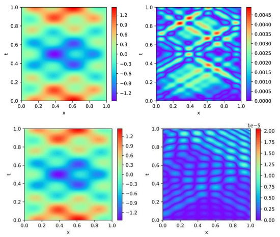
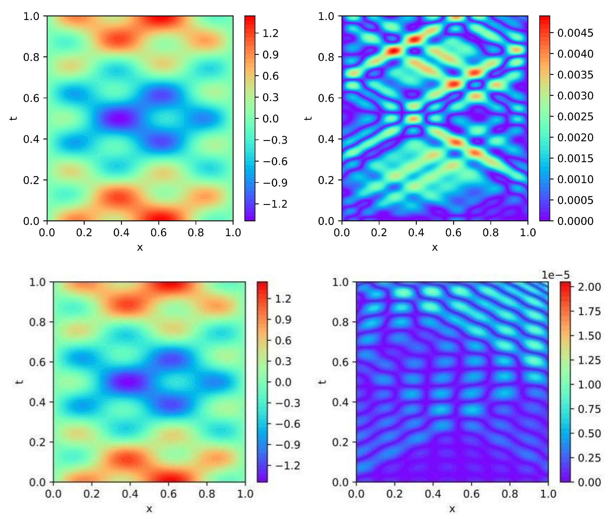
Figure 3 presents the numerical solutions and associated error plots for the proposed dual-PINN’s framework under two optimizers: Adam and L-BFGS.

Figure 3. Predicted solutions and pointwise absolute errors for Example 1 using the Dual-PINN trained with Adam (top) and L-BFGS (bottom). The reference solution is the prescribed analytical solution.

5.3. Example 2: One-Dimensional Boundary-Reflection Problem

We next consider the one-dimensional wave equation

$$u_{tt}(x,t)-c^2{u}_{xx}(x,t)=0,(x,t)\in (0,2)\times (0,t_f],$$

(53)

with

$$u(x,0)=0.5\exp [-100{(x-1)}^2],u_t(x,0)=0,$$

(54)

and homogeneous Dirichlet boundary conditions

$$u(0,t)=u(2,t)=0.$$

(55)

The wave speed is given by

$$c=\sqrt{{\displaystyle \frac{T}{\mu }}},$$

(56)

where T denotes the tension of the string and $\mu$ denotes its linear mass density, i.e., the mass per unit length, $c^2=0.02$.

To satisfy the homogeneous Dirichlet conditions exactly, the prediction is written as

$$\widehat{u}(x,t)=x(2-x)\left[{\mathcal{N}}_{+}(x-ct;{\theta }_{+})+{\mathcal{N}}_{-}(x+ct;{\theta }_{-})\right].$$

(57)

The Dual-PINN contains two branches, each with two hidden layers and 20 neurons per layer. A total of 5000 interior collocation points and 500 initial points are used. The weights for different loss terms are empirically set as ${\omega }_r=0.1,{\omega }_0=1,{\omega }_b=1,{\omega }_d=0$.

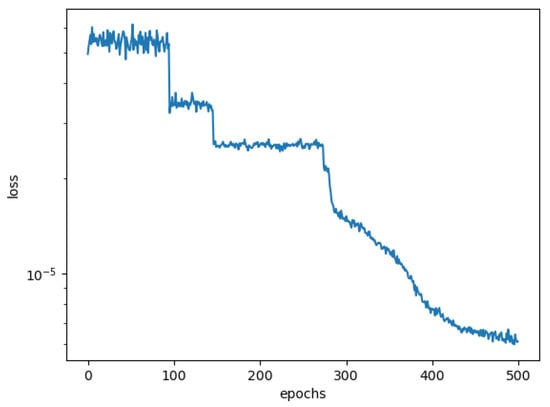
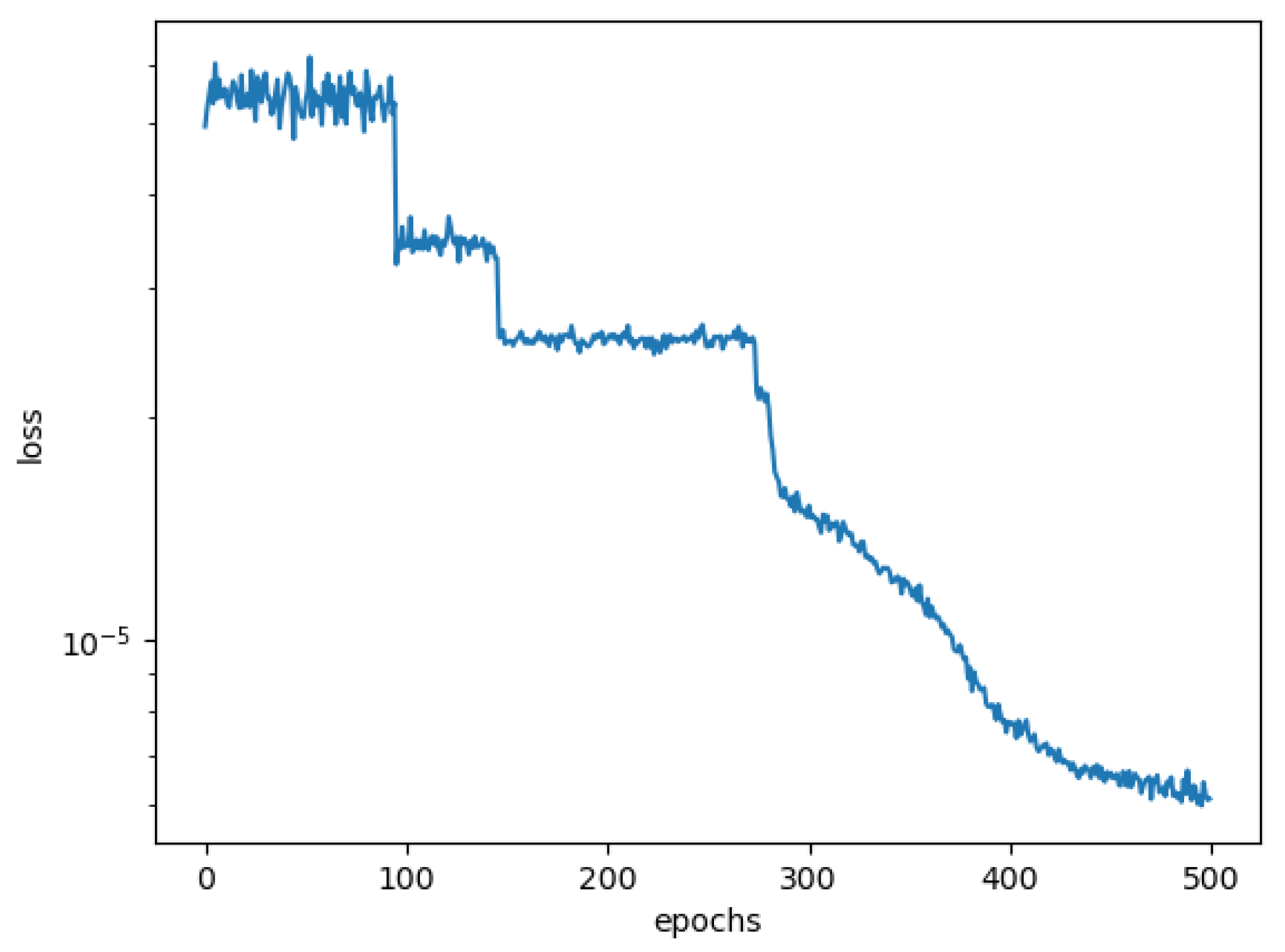
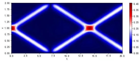
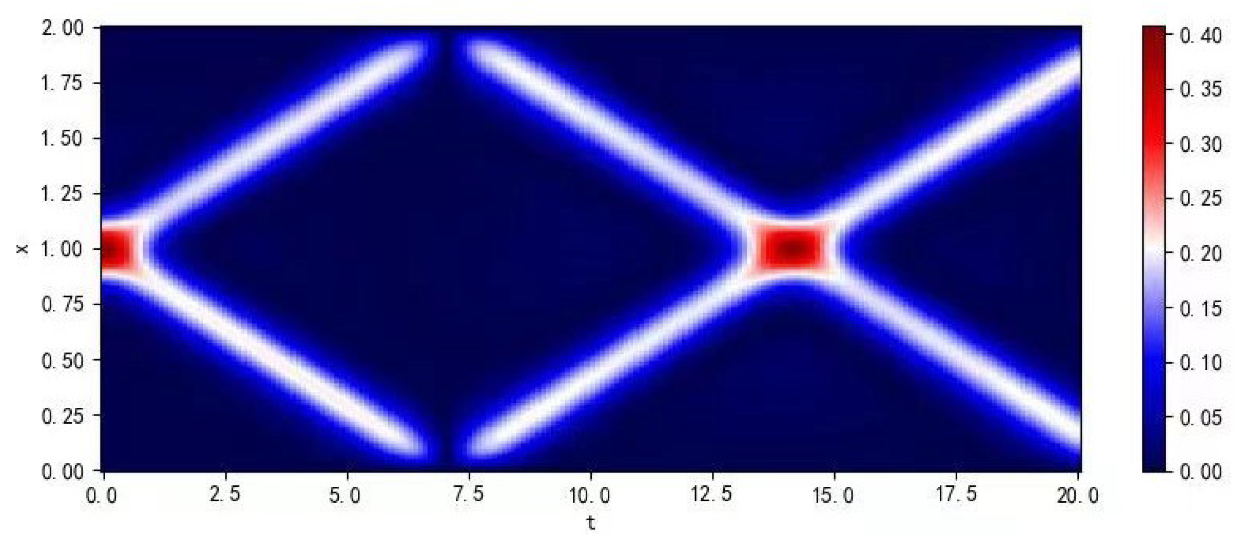
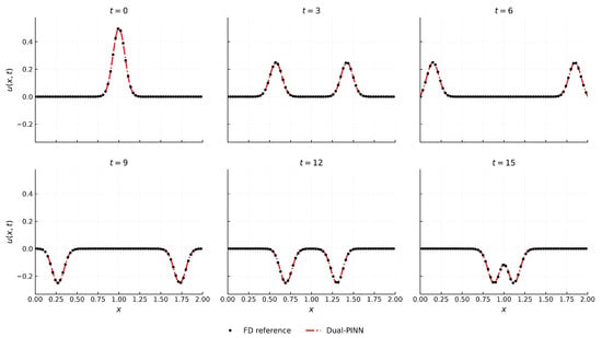
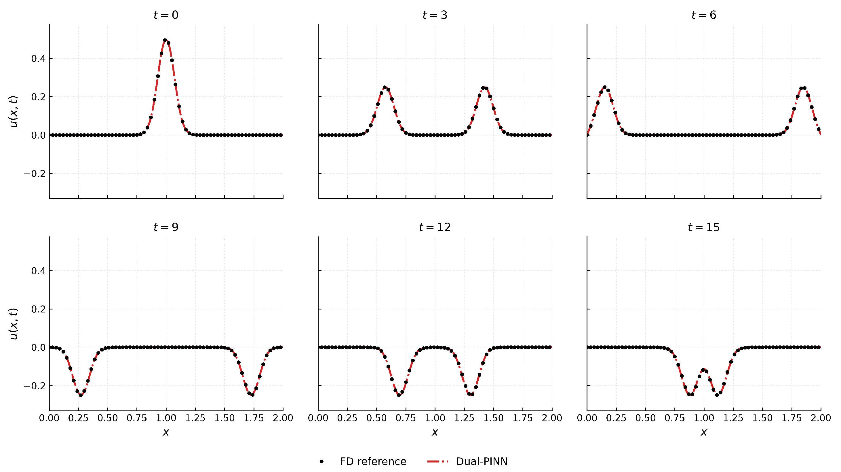
Figure 4 shows the evolution of the training loss, while Figure 5 presents the predicted spatiotemporal solution of the one-dimensional wave problem. Figure 6 compares the Dual-PINN prediction with the finite-difference reference solution at different time instants. The predicted solution agrees well with the reference during both incident-wave propagation and subsequent boundary reflection, indicating that the Dual-PINN captures the principal propagation and reflection structures in this test case.

Figure 4. The evolution of loss function during iteration.

Figure 5. The solutions of one-dimensional wave equation obtained by our dual-PINNs.

Figure 6. Spatiotemporal evolution of the solution $u(x,t)$ comparing the Finite Difference (FD) reference solution (black dots) and the Dual-Physics Informed Neural Network (Dual-PINN) prediction (red dash-dotted line). The snapshots display the wave propagation and interaction at time steps $t=0,3,6,9,12,$ and 15.

5.4. Example 3: Two-Dimensional Wave Problem

Finally, we consider the two-dimensional wave equation

$$u_{tt}=c^2\left(u_{xx}+u_{yy}\right),(x,y)\in (0,2)\times (0,2),$$

(58)

with the initial conditions

$$u(x,y,0)=0.5\exp \left(-100[{(x-1)}^2+{(y-1)}^2]\right),u_t(x,y,0)=0,$$

(59)

and homogeneous Dirichlet boundary conditions on $\partial \mathrm{\Omega }$, $c^2=0.02$.

For this numerical extension, the homogeneous boundary conditions are enforced through the trial representation

$$\widehat{u}(x,y,t)=x(2-x)y(2-y){\mathcal{D}}_{\mathrm{\Theta }}(x,y,t),$$

(60)

where ${\mathcal{D}}_{\mathrm{\Theta }}$ denotes the dual-network representation used for the two-dimensional experiment. As clarified in Section 3 and Section 4, this 2D formulation is treated as a numerical extension and is not covered by the exact one-dimensional d’Alembert decomposition.

For a consistent comparison, the conventional PINN employs a single network with three hidden layers of 80 neurons each, whereas the Dual-PINN consists of two parallel branches, each containing three hidden layers of 40 neurons, resulting in the same total number of hidden neurons for both methods.

To better represent the approximately radial propagation of the initially localized Gaussian pulse, we introduce

$$r=\sqrt{{(x-1)}^2+{(y-1)}^2},$$

and augment the two branches with $r-ct$ and $r+ct$, respectively. These quantities are used solely as physics-motivated auxiliary features in the two-dimensional experiment rather than as exact characteristic coordinates.

Accordingly, the inputs to the two branches are defined as

$$(x_n,y_n,t_n,{(r-ct)}_n)$$

and

$$(x_n,y_n,t_n,{(r+ct)}_n),$$

respectively, where the subscript n denotes normalized variables.

A total of $N_i=20,000$ interior points, $N_0=1000$ initial-condition points, and $N_b=1200$ boundary points are used. The sampling combines global, locally refined, temporally stratified, and reflection-focused points, with additional late-time refinement near the boundaries. L-BFGS training follows a three-stage temporal curriculum with 500, 750, and 1750 iterations on $t\in [0,4]$, $[0,7]$, and $[0,10]$, respectively, totaling 3000 iterations. Finite-difference snapshots at $t=0,2,4,6,$ and 8 are further incorporated through the data-loss term ${\mathcal{L}}_d$ in Equation (35), while $t=10$ is reserved for out-of-sample temporal evaluation. The same data and training settings are used for the PINN and Dual-PINN.

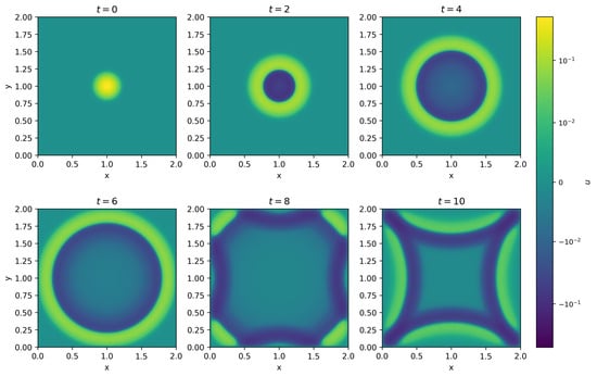
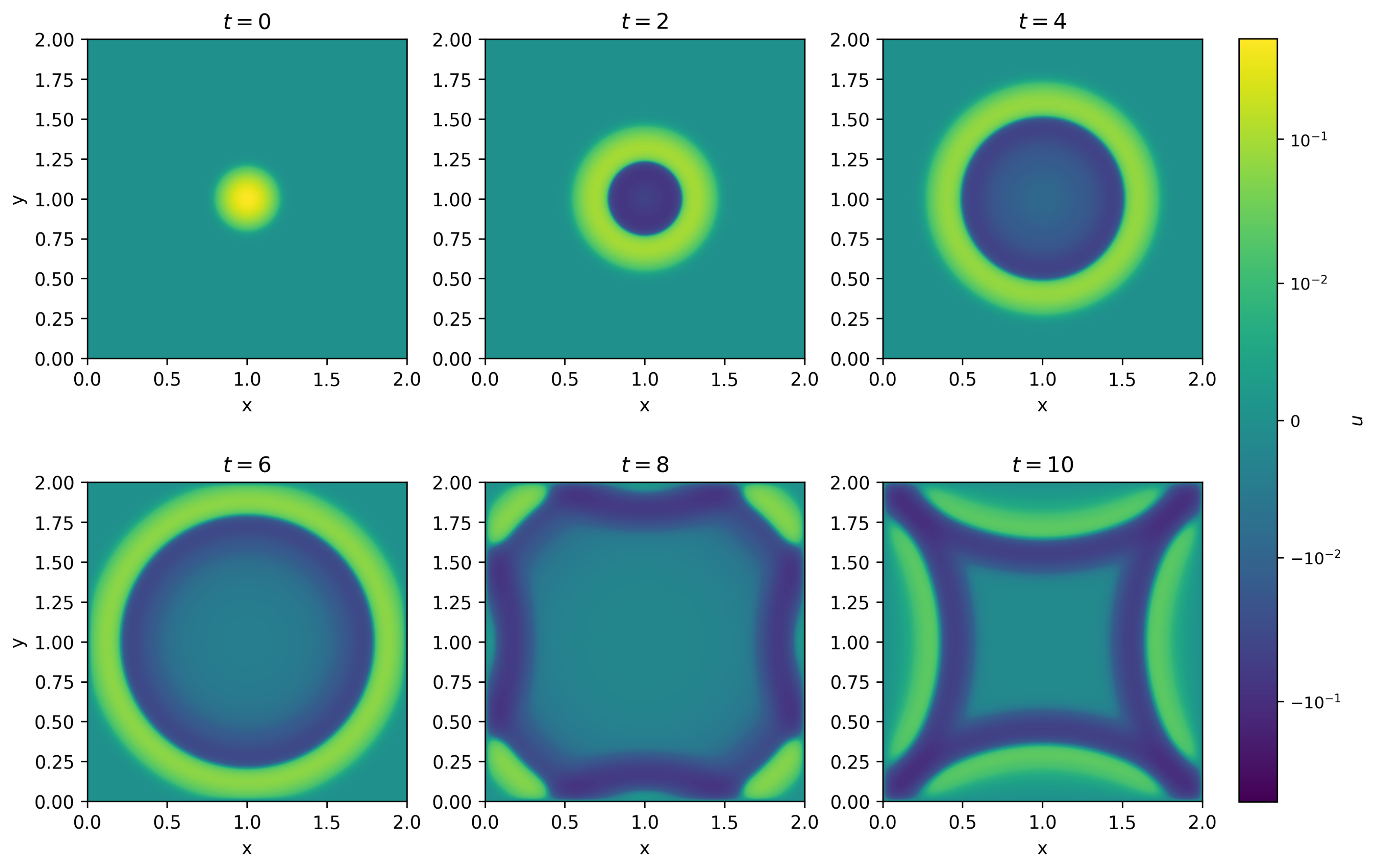
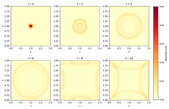
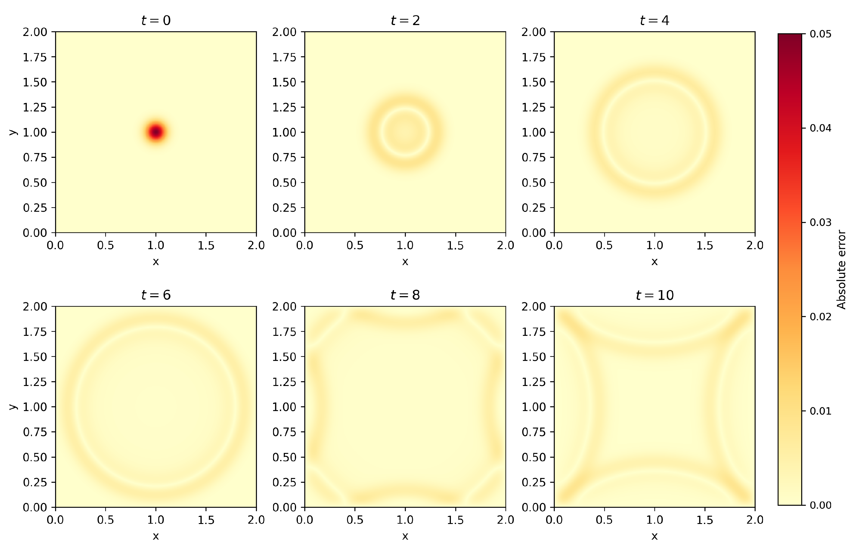
Figure 7 and Figure 8 show the predicted wave fields and the corresponding pointwise absolute errors at six representative times. The Dual-PINN accurately captures the outward propagation of the initial pulse and the subsequent boundary-interaction patterns. The errors are primarily localized near the moving wavefronts and reflected structures, while the remaining regions retain relatively small discrepancies. This behavior demonstrates that the proposed representation can preserve the principal two-dimensional wave dynamics over the considered time interval.

Figure 7. Dual-PINN predictions for the two-dimensional wave equation at $t=0,2,4,6,8,$ and 10.

Figure 8. Pointwise absolute errors of the Dual-PINN predictions for the two-dimensional wave equation at $t=0,2,4,6,8,$ and 10, computed with respect to the finite-difference reference solution.

Table 4 further quantifies the prediction accuracy in Example 3. The relative $L_2$ error of PINN increases from $5.5\times {10}^{-2}$ at $t=2$ to $3.8\times {10}^{-1}$ at $t=10$, whereas Dual-PINN maintains considerably smaller errors over the entire interval, with $E_{\mathrm{rel},2}=6.1\times {10}^{-2}$ at $t=10$. Moreover, Dual-PINN uses only 7042 trainable parameters compared with $13,361$ for PINN. This comparison indicates that the dual-branch representation improves the accuracy–complexity trade-off for the present two-dimensional wave problem, particularly during the later-time wave-reflection stage.

Table 4. Quantitative comparison of PINN and Dual-PINN for the two-dimensional wave problem at representative time instants.

Method	Metric	$\mathit{t}=2$	$\mathit{t}=4$	$\mathit{t}=6$	$\mathit{t}=8$	$\mathit{t}=10$	Params.	Training Time
PINN	Rel. $L_2$	$5.5\times {10}^{-2}$	$8.5\times {10}^{-2}$	$1.3\times {10}^{-1}$	$2.3\times {10}^{-1}$	$3.8\times {10}^{-1}$	13,361	2526.6
	Max.	$6.9\times {10}^{-2}$	$7.5\times {10}^{-2}$	$1.9\times {10}^{-1}$	$2.5\times {10}^{-1}$	$5.6\times {10}^{-1}$
Dual-PINN	Rel. $L_2$	$4.2\times {10}^{-3}$	$8.3\times {10}^{-3}$	$2.1\times {10}^{-2}$	$2.8\times {10}^{-2}$	$6.1\times {10}^{-2}$	7042	1427.9
	Max.	$6.6\times {10}^{-3}$	$9.0\times {10}^{-3}$	$3.6\times {10}^{-2}$	$5.2\times {10}^{-2}$	$7.6\times {10}^{-2}$

6. Conclusions

This work develops a Dual Physics-Informed Neural Network (Dual-PINN) for wave-equation problems with particular emphasis on boundary reflection. For the one-dimensional linear wave equation, the proposed architecture uses two neural branches associated with the characteristic coordinates $x-ct$ and $x+ct$ to represent counter-propagating wave components. Their outputs are combined and jointly constrained by the governing equation and the prescribed initial and boundary conditions. For the homogeneous Dirichlet reflection problems, the boundary conditions are further enforced through a problem-specific trial function. This structured representation provides a direct way to incorporate the traveling-wave decomposition into the neural approximation.

The numerical experiments show that the method can reproduce the tested periodic-wave and boundary-reflection solutions with controlled errors. The network-sensitivity study shows that the configuration with two hidden layers and 20 neurons per layer achieves a relative $L_2$ error of $1.19\times {10}^{-3}$ and a maximum error of $2.36\times {10}^{-3}$, with a training time of $49.9$ s. This configuration therefore provides a favorable balance between prediction accuracy and computational cost for Example 1.

The present formulation also has several limitations. The theoretical result applies only to the one-dimensional characteristic representation, whereas the two-dimensional formulation should be interpreted as an empirical numerical extension rather than a consequence of Proposition 1. In addition, the performance of the method remains dependent on network architecture, sampling, loss weighting, and optimization. Future work will therefore focus on constructing multidimensional directional decompositions, extending the branch representation to heterogeneous media with spatially varying wave speeds, and developing adaptive branch-coupling and sampling strategies for more challenging long-time wave-propagation problems.

References

- Dablain, M.A. The application of high-order differencing to the scalar wave equation. Geophysics 1986, 51, 54–66. [Google Scholar] [CrossRef] [Scilit]
- Liu, Y.; Sen, M.K. A new time-pace domain high-order finite-difference method for the acoustic wave equation. J. Comput. Phys. 2009, 228, 8779–8806. [Google Scholar] [CrossRef] [Scilit]
- Grote, M.J.; Schneebeli, A.; Schtzau, D. Discontinuous Galerkin finite element method for the wave equation. Siam J. Numer. Anal. 2006, 44, 2408–2431. [Google Scholar] [CrossRef] [Scilit]
- Guo, B.Y. Spectral Methods and Their Applications; World Scientific: Singapore, 1998. [Google Scholar]
- Ainsworth, M.; Monk, P.; Muniz, W. Dispersive and dissipative properties of discontinuous Galerkin finite element methods for the second-order wave equation. J. Sci. Comput. 2006, 27, 5–40. [Google Scholar] [CrossRef] [Scilit]
- Wang, S. An improved high order finite difference method for non-conforming grid interfaces for the wave equation. J. Sci. Comput. 2018, 77, 775–792. [Google Scholar] [CrossRef] [Scilit]
- Colombi, A.; Nissen-Meyer, T.; Boschi, L.; Giardini, D. Seismic waveform sensitivity to global boundary topography. Geophys. J. Int. 2012, 191, 832–848. [Google Scholar] [CrossRef] [Scilit]
- Tesoniero, A.; Leng, K.; Long, D.M.; Nissen-Meyer, T. Full wave sensitivity of SK (K) S phases to arbitrary anisotropy in the upper and lower mantle. Geophys. J. Int. 2020, 222, 412–435. [Google Scholar] [CrossRef] [Scilit]
- Moseley, B.; Markham, A.; Nissen-Meyer, T. Solving the wave equation with physics-informed deep learning. arXiv 2020, arXiv:2006.11894. [Google Scholar] [CrossRef] [Scilit]
- Rashtehesht, M.; Huber, C.; Shukla, K.; Karniadakis, G.E. Physics-informed neural networks (PINNs) for wave propagation and full waveform inversions. J. Geophys. Res. Solid Earth 2022, 127, e2021JB023120. [Google Scholar] [CrossRef] [Scilit]
- Srinivasa, K.; Mulimani, M.; Adel, W. A numerical approach for solving nonlinear fractional Klein–Gordon equation with applications in quantum mechanics. J. Nonlinear Complex Data Sci. 2024, 25, 173–195. [Google Scholar] [CrossRef] [Scilit]
- Nguyen, H.; Tsai, R. Numerical wave propagation aided by deep learning. J. Comput. Phys. 2023, 475, 111828. [Google Scholar] [CrossRef] [Scilit]
- Raissi, M.; Perdikaris, P.; Karniadakis, G.E. Physics-informed neural networks: A deep learning framework for solving forward and inverse problems involving nonlinear partial differential equations. J. Comput. Phys. 2019, 378, 686–707. [Google Scholar] [CrossRef] [Scilit]
- Cai, S.; Mao, Z.; Wang, Z.; Yin, M.; Karniadakis, G.E. Physics-informed neural networks (PINNs) for fluid mechanics: A review. Acta Mech. Sin. 2021, 37, 1727–1738. [Google Scholar] [CrossRef] [Scilit]
- Wang, S.; Teng, Y.; Perdikaris, P. Understanding and mitigating gradient flow pathologies in physics-informed neural networks. Siam J. Sci. Comput. 2021, 43, A3055–A3081. [Google Scholar] [CrossRef] [Scilit]
- Wang, S.; Yu, X.; Perdikaris, P. When and why PINNs fail to train: A neural tangent kernel perspective. J. Comput. Phys. 2022, 449, 110768. [Google Scholar] [CrossRef] [Scilit]
- Krishnapriyan, A.S.; Gholami, A.; Zhe, S.; Kirby, R.M.; Mahoney, M.W. Characterizing possible failure modes in physics-informed neural networks. Adv. Neural Inf. Process. Syst. 2021, 34, 26548–26560. [Google Scholar]
- Song, J.; Zhong, M.; Karniadakis, G.E.; Yan, Z. Two-stage initial-value iterative physics-informed neural networks for simulating solitary waves of nonlinear wave equations. J. Comput. Phys. 2024, 505, 112917. [Google Scholar] [CrossRef] [Scilit]
- Jagtap, A.D.; Kawaguchi, K.; Em Karniadakis, G. Locally adaptive activation functions with slope recovery for deep and physics-informed neural networks. Proc. R. Soc. A 2020, 476, 20200334. [Google Scholar] [CrossRef] [Scilit]
- Jagtap, A.D.; Kawaguchi, K.; Karniadakis, G.E. Adaptive activation functions accelerate convergence in deep and physics-informed neural networks. J. Comput. Phys. 2020, 404, 109136. [Google Scholar] [CrossRef] [Scilit]
- Nosrati, H.; Emami Niri, M. Manipulating the loss calculation to enhance the training process of physics-informed neural networks to solve the 1D wave equation. Eng. Comput. 2024, 40, 1741–1769. [Google Scholar] [CrossRef] [Scilit]
- Alkhadhr, S.; Almekkawy, M. Modeling the Wave Equation Using Physics-Informed Neural Networks Enhanced With Attention to Loss Weights. In Proceedings of the ICASSP 2023—2023 IEEE International Conference on Acoustics, Speech and Signal Processing, Rhodes Island, Greece, 4–10 June 2023; pp. 4438–4442. [Google Scholar]
- Maczuga, P.; Paszyiski, M. Influence of activation functions on the convergence of physics-informed neural networks for 1D wave equation. In International Conference on Computational Science; Springer Nature: Cham, Switzerland, 2023; pp. 74–88. [Google Scholar]
- Alkhadhr, S.; Almekkawy, M. Wave equation modeling via physics-informed neural networks: Models of soft and hard constraints for initial and boundary conditions. Sensors 2023, 23, 2792. [Google Scholar] [CrossRef] [Scilit]
- Lin, S.; Chen, Y. A two-stage physics-informed neural network method based on conserved quantities and applications in localized wave solutions. J. Comput. Phys. 2022, 457, 111053. [Google Scholar] [CrossRef] [Scilit]
- Song, C.; Wang, Y. Simulating seismic multifrequency wavefields with the Fourier feature physics-informed neural network. Geophys. J. Int. 2023, 232, 1503–1514. [Google Scholar] [CrossRef] [Scilit]
- Wu, T.; Zhao, C.; Liu, X. IS-PINN: Integrating mathematical principles to solve inhomogeneous wave equations via physics-informed neural networks. Comput. Math. Appl. 2025, 193, 177–204. [Google Scholar] [CrossRef] [Scilit]
- Liu, Y.; Zhang, X.; Dong, Q.; Chen, G.; Li, X. Phase-resolved wave prediction with linear wave theory and physics-informed neural networks. Appl. Energy 2024, 355, 121602. [Google Scholar] [CrossRef] [Scilit]
- Qi, S.; Sarris, C.D. Hybrid physics-informed neural network for the wave equation with unconditionally stable time-stepping. IEEE Antennas Wirel. Propag. Lett. 2024, 23, 1356–1360. [Google Scholar] [CrossRef] [Scilit]
- Jagtap, A.D.; Karniadakis, G.E. Extended physics-informed neural networks (XPINNs): A generalized space-time domain decomposition based deep learning framework for nonlinear partial differential equations. Commun. Comput. Phys. 2020, 28, 2002–2041. [Google Scholar] [CrossRef] [Scilit]
- Sukumar, N.; Srivastava, A. Exact imposition of boundary conditions with distance functions in physics-informed deep neural networks. Comput. Methods Appl. Mech. Eng. 2022, 389, 114333. [Google Scholar] [CrossRef] [Scilit]
- Van Der Meer, R.; Oosterlee, C.W.; Borovykh, A. Optimally weighted loss functions for solving pdes with neural networks. J. Comput. Appl. Math. 2022, 405, 113887. [Google Scholar] [CrossRef] [Scilit]
- McClenny, L.D.; Braga-Neto, U.M. Self-adaptive physics-informed neural networks. J. Comput. Phys. 2023, 474, 111722. [Google Scholar] [CrossRef] [Scilit]
Disclaimer/Publisher’s Note: The statements, opinions and data contained in all publications are solely those of the individual author(s) and contributor(s) and not of MDPI and/or the editor(s). MDPI and/or the editor(s) disclaim responsibility for any injury to people or property resulting from any ideas, methods, instructions or products referred to in the content. |
© 2026 by the authors. Licensee MDPI, Basel, Switzerland. This article is an open access article distributed under the terms and conditions of the Creative Commons Attribution (CC BY) license.