A Novel Full NT-Step Infeasible Interior-Point Algorithm for Semi-Definite Linear Complementarity Problems: Convergence and Numerical Performance

Abstract

This paper presents an improved infeasible interior-point algorithm tailored for semi-definite linear complementarity problems (SDLCPs). The proposed approach leverages full Nesterov–Todd search directions while eliminating centering steps, significantly simplifying the algorithmic structure and reducing computational overhead. A rigorous theoretical analysis confirms that the method is well defined, globally convergent, and achieves an iteration complexity that matches the best-known bounds for infeasible interior-point methods in this domain. Complementing the theoretical results, extensive numerical experiments highlight the algorithm’s superior practical performance, consistently achieving faster convergence with fewer iterations compared to existing methods. These findings demonstrate the algorithm’s potential as an efficient and robust solution technique for SDLCPs, with promising applicability to large-scale and complex problem instances.

1. Introduction

Let ${\mathbb{S}}^n$ be the set of all $n\times n$ real symmetric matrices, and let ${\mathbb{S}}_{+}^n$ be the set of all positive semi-definite matrices in ${\mathbb{S}}^n$. Given a linear operator $\mathcal{L}:{\mathbb{S}}^n\to {\mathbb{S}}^n$ and a matrix $Q\in {\mathbb{S}}^n$, the semi-definite linear complementarity problem (SDLCP) is to find matrices $X,Y\in {\mathbb{S}}^n$ such that:

$$X,Y\in {\mathbb{S}}_{+}^n,Y=\mathcal{L}\left(X\right)+Q,X•Y=0,$$

(1)

where $X•Y=\mathrm{Tr}\left(XY\right)$ is the trace inner product. The operator $\mathcal{L}$ is assumed to be symmetric and positive semi-definite.

The Semi-definite Linear Complementarity Problem represents a broad class of optimization problems that encompasses several well-known formulations, including the standard Linear Complementarity Problem (LCP), semi-definite programming (SDP), and systems of matrix inequalities. Owing to its generality, SDLCP finds applications in diverse areas such as control theory and the analysis of systems characterized by linear or bilinear inequalities. Moreover, the framework of SDLCP also extends to encompass variants such as the geometric version of the problem, thereby enhancing its relevance across multiple domains (see [1,2]).

Over the years, numerous methods have been proposed to address SDLCP, with interior-point methods (IPMs) emerging as some of the most effective approaches. Initially developed for solving linear optimization problems, IPMs have demonstrated remarkable success in handling more complex problem classes, including quadratic optimization, semi-definite optimization, and SDLCP itself (see [3,4,5,6,7,8,9,10]).

Consequently, several symmetrized search directions have been proposed in the literature to enhance the performance of interior-point algorithms [11,12,13,14]. Among these, the Alizadeh–Haeberly–Overton (AHO), Helmberg–Kojima–Monteiro (HKM), and Nesterov–Todd (NT) directions are the most prominent. Notably, the HKM and NT directions have been widely adopted in state-of-the-art semi-definite programming solvers, such as SeDuMi and SDPT3, reflecting their practical effectiveness.

Extensive research has investigated the performance and convergence properties of primal–dual path-following interior-point algorithms employing the HKM direction, establishing its significance in the field. Furthermore, infeasible interior-point methods (IPMs) have been developed to overcome the limitations of requiring feasible initial points. These methods can start from any positive point, simultaneously progressing toward feasibility and optimality. The efficiency of IPMs, however, is highly sensitive to the choice of the starting point. Lustig [15] was the first to introduce infeasible interior-point methods (IPMs) for linear optimization. Later, Zhang [16] developed the first primal–dual IPM for semi-definite optimization (SDO) with a proven polynomial iteration complexity (see references [17,18]).

This paper presents an infeasible interior-point method (IIPM) for semi-definite linear complementarity problems (SDLCPs) based on a full Nesterov–Todd (NT) step without centering. Although this approach has already been studied in semi-definite programming (SDP), extending it to SDLCP requires a separate convergence analysis that takes into account the structure of the problem and its complementarity conditions. The main contribution of this work is to adapt the approach to SDLCP and establish its convergence properties. We also derive an iteration complexity bound of $\mathcal{O}\left(n\log {\epsilon }^{-1}\right)$ and present numerical experiments to evaluate the performance of the proposed algorithm.

The paper is organized as follows:

• Section 2 provides the necessary definitions and background.
• Section 3 introduces the Newton search directions for SDLCP.
• Section 4 details the proposed infeasible interior-point algorithm for SDLCP.
• Section 5 presents the convergence analysis of the algorithm.
• Section 6 reports the numerical results validating the theoretical findings.
• Section 7 concludes the study with final remarks and potential future research directions.

Notation: The notation $X\succ 0$ means that X is positive-definite. The smallest and largest eigenvalues of a matrix V are denoted by ${\lambda }_{\min }\left(V\right)$ and ${\lambda }_{\max }\left(V\right)$. The Frobenius norm is written as ${\parallel X\parallel }_F$:

$${\parallel X\parallel }_F:=\sqrt{\mathrm{Tr}\left(X{X}^T\right)}{,\parallel X\parallel }_2:=\underset{i}{\max }\left|{\lambda }_i\left(X\right)\right|.$$

The identity matrix is denoted by I. The set of all $m\times n$ real matrices is represented by ${\mathbb{R}}^{m\times n}$, while ${\mathbb{S}}^n$ denotes the set of all $n\times n$ real symmetric matrices. Furthermore, ${\mathbb{S}}_{++}^n$ and ${\mathbb{S}}_{+}^n$ represent the sets of symmetric positive-definite and positive-semi-definite matrices, respectively. For any matrix $A\in {\mathbb{S}}^n$, the determinant and trace are defined as:

$$\det \left(A\right):={\displaystyle \prod _{i=1}^n}{\lambda }_i\left(A\right),\mathbf{Tr}\left(A\right):={\displaystyle \sum _{i=1}^n}{\lambda }_i\left(A\right).$$

where ${\lambda }_i\left(A\right)$ are the eigenvalues of A. If $A\in {\mathbb{S}}_{++}^n$ is symmetric and positive-definite, its matrix square root is denoted by $A^{1/2}$. Finally, two matrices A and B are said to be similar, denoted $A\sim B$, if there exists an invertible matrix Q such that: $A=QB{Q}^{-1}$.

2. Preliminary Notations and Tools

This section establishes the fundamental definitions and key lemmas that form the mathematical foundation for the proposed algorithm. These preliminaries are essential for developing the theoretical results presented in the later sections. The notation and framework adopted here largely follow the treatments provided in [19,20].

2.1. Some Results on Matrices and Matrix Functions

Lemma 1

(See [19]). Let $X,Y\in {\mathbb{S}}_{+}^n$. Then the following conditions are equivalent:

1.

$X•Y=0$;

2.

$XY=0$;

3.

${\displaystyle \frac{XY+YX}{2}}=0$.

The Kronecker product between two matrices A and B is denoted by $A\otimes B$ and forms a structured block matrix. For a matrix $A\in {\mathbb{R}}^{n\times n}$, we define the vectorization operator $\mathrm{vec}$, which converts A into a column vector of dimension $n^2$, as follows:

$$\mathrm{vec}\left(A\right)={(a_{11},a_{21},\dots ,a_{n1},a_{12},\dots ,a_{n2},\dots ,a_{nn})}^{\top }.$$

We also introduce the symmetric vectorization operator $\mathrm{svec}$, which maps a symmetric matrix $A\in {\mathbb{S}}^n$ to a vector in ${\mathbb{R}}^{{\displaystyle \frac{n(n+1)}{2}}}$ by accounting for symmetry:

Definition 1.

Let $A\in {\mathbb{S}}^n$. Then the operator $\mathrm{svec}\left(A\right)$ is defined as:

$$\mathrm{svec}\left(A\right)={(a_{11},\sqrt{2}{a}_{21},\dots ,\sqrt{2}{a}_{n1},a_{22},\sqrt{2}{a}_{32},\dots ,\sqrt{2}{a}_{n2},\dots ,a_{nn})}^{\top }.$$

Its inverse is denoted by $\mathrm{smat}$ and satisfies:

$$\mathrm{smat}\left(\mathrm{svec}\right(A\left)\right)=A.$$

Definition 2.

Let $V\in {\mathbb{S}}_{+}^n$ and

$$V=Q^{T}diag({\lambda }_1\left(V\right),{\lambda }_2\left(V\right),\dots ,{\lambda }_n\left(V\right))Q,$$

where Q is any orthonormal matrix $(Q^T=Q^{-1})$ that diagonalizes V. The matrix valued function $\psi \left(V\right)$ is defined by

$$\psi \left(V\right)=Q^{T}diag(\psi \left({\lambda }_1\left(V\right)\right),\psi \left({\lambda }_2\left(V\right)\right),\dots ,\psi \left({\lambda }_n\left(V\right)\right))Q.$$

(2)

It should be noted that the matrix Q is not unique, but $\psi \left(V\right)$ is well defined whenever $\psi \left(t\right)$ is well defined on the eigenvalues of V.

Furthermore, replacing $\psi \left({\lambda }_l\left(V\right)\right)$ in (2) by ${\psi }^{\prime }\left({\lambda }_l\left(V\right)\right)$, we can conclude that the matrix functions $\psi \left(V\right)$

$${\psi }^{\prime }\left(V\right)=Q^{T}diag({\psi }^{\prime }\left({\lambda }_1\left(V\right)\right),{\psi }^{\prime }\left({\lambda }_2\left(V\right)\right),\dots ,{\psi }^{\prime }\left({\lambda }_n\left(V\right)\right))Q,$$

(3)

are defined as well.

Definition 3.

A matrix $X\left(t\right)$ is said to be a matrix of functions if each entry of $X\left(t\right)$ is a function of t, that is, $X\left(t\right)=\left[X_{ij}\left(t\right)\right]$. The concepts of continuity, differentiability and integrability naturally extend to matrix-valued functions of a scalar by interpreting them component-wise. Thus we can say that

$${\displaystyle \frac{d}{dt}}X\left(t\right)={\displaystyle \frac{d}{dt}}\left[X_{ij}\left(t\right)\right]=X^{\prime }\left(t\right).$$

Suppose that the matrix-valued functions $H\left(t\right)$ and $G\left(t\right)$ are differentiable with respect to t. Then we have

$$\begin{array}{ccc}\hfill {\displaystyle \frac{d}{dt}}\left(\mathit{Tr}\left(G\left(t\right)\right)\right)& =& \mathit{Tr}\left({\displaystyle \frac{d}{dt}}G\left(t\right)\right)=\mathit{Tr}\left(G^{\prime }\left(t\right)\right)\hfill \\ \hfill {\displaystyle \frac{d}{dt}}\left(G\left(t\right)H\left(t\right)\right)& =& G^{\prime }\left(t\right)H\left(t\right)+G\left(t\right)H^{\prime }\left(t\right).\hfill \end{array}$$

For any function $\psi \left(t\right)$, let us denote by $▵\psi \left(t\right)$ the divided difference of $\psi \left(t\right)$:

$$▵\psi (t_1,t_2)={\displaystyle \frac{\psi \left(t_1\right)-\psi \left(t_2\right)}{t_1-t_2}},\forall t_1\ne t_2;$$

if $t_1=t_2$ then we simply write $▵\psi (t_1,t_2)={\psi }^{\prime }\left(t\right)$.

Lemma 2.

Suppose that $H\left(t\right)$ is a matrix of functions such that the matrix $H\left(t\right)$ is positive-definite with eigenvalues ${\lambda }_1\left(t\right)\ge {\lambda }_2\left(t\right)\ge \cdots ,{\lambda }_n\left(t\right)>0$. If $H\left(t\right)$ is twice differentiable with respect to $t\in (l_t,u_t)$ and $\psi \left(t\right)$ is twice continuously differentiable function in a domain that contains all the eigenvalues of $H\left(t\right)$ then

$$\begin{array}{ccc}\hfill {\displaystyle \frac{d}{dt}}\mathit{Tr}(\psi \left(H\left(t\right)\right)& =& \mathit{Tr}({\psi }^{\prime }\left(H\left(t\right)H^{\prime }\left(t\right)\right),\hfill \\ \hfill {\displaystyle \frac{d^2}{d{t}^2}}\mathit{Tr}(\psi \left(H\left(t\right)\right)& \le & \omega {∥H^{\prime }\left(t\right)∥}^2+\mathit{Tr}({\psi }^{\prime }\left(H\left(t\right)H^{\prime \prime }\left(t\right)\right),\hfill \end{array}$$

where

$$\omega =\max \left\{\left|\Delta {\psi }^{\prime }({\lambda }_j\left(t\right),{\lambda }_k\left(t\right))\right|:t\in (l_t,u_t),j,k=1,2,\dots ,n\right\}$$

is a number depending on $H^{\prime }\left(t\right)$ and $\psi \left(t\right)$ with

$$\Delta {\psi }^{\prime }(t_1,t_2)={\displaystyle \frac{{\psi }^{\prime }\left(t_1\right)-{\psi }^{\prime }\left(t_2\right)}{t_1-t_2}},\forall t_1,t_2\in \left[l_t,u_t\right].$$

2.2. Central Path of Perturbed Problems

We now define the feasible region of the problem. Let $\mathcal{L}\left(X\right)$ be symmetric and positive semi-definite, and $Q\in {\mathbb{S}}^n$. The feasible set and its strictly feasible subset are given by:

$$\begin{array}{cc}\hfill {\mathcal{F}}_P& =\left\{(X,Y)|X\in {\mathbb{S}}_{+}^n,Y\in {\mathbb{S}}_{+}^n,Y=\mathcal{L}\left(X\right)+Q\right\},\hfill \\ \hfill {\mathcal{F}}_P^0& =\left\{(X,Y)\in {\mathcal{F}}_P|X\in {\mathbb{S}}_{++}^n,Y\in {\mathbb{S}}_{++}^n\right\}.\hfill \end{array}$$

The sets of optimal solutions for the primal–dual problem, assuming the optimal value $p^{\star }$ is attained, are defined as:

$$\begin{array}{cc}\hfill {\mathcal{S}}_P^{\mathrm{opt}}& =\left\{Y\in {\mathbb{S}}_{+}^n|\exists X\in {\mathbb{S}}_{+}^n:Y=\mathcal{L}\left(X\right)+Q,f\left(Y\right)=p^{\star }\right\},\hfill \end{array}$$

We make the following assumptions throughout the development of the algorithm:

• The set ${\mathcal{F}}_P^0$ is non-empty,
• The linear operator $\mathcal{L}:{\mathbb{S}}^n\to {\mathbb{S}}^n$ is monotone and self-adjoint. That is, for all $X,Y\in {\mathbb{S}}^n$,

$$X•\mathcal{L}\left(X\right)\ge 0\mathrm{and}X•\mathcal{L}\left(Y\right)=\mathcal{L}\left(X\right)•Y.$$

The existence of a solution to the SDLCP (1) is considered under the assumptions stated above. Since $X,Y\in {\mathbb{S}}_{+}^n$, the condition $⟨X,Y⟩=0$ is equivalent to $XY=0$. Therefore, finding a solution of (1) is equivalent to solving the following system:

$$\left\{\begin{array}{c}Y-\mathcal{L}\left(X\right)-Q=0,\hfill \\ XY=0,X,Y⪰0.\hfill \end{array}\right.$$

(4)

The basic idea of primal–dual IPMs is to replace the second equation in (4) by the parameterized equation $XY=\mu I$, $\mu >0$. Hence, we consider the following system:

$$\left\{\begin{array}{c}Y-\mathcal{L}\left(X\right)-Q=0,\hfill \\ XY=\mu I,X,Y⪰0.\hfill \end{array}\right.$$

(5)

Under the assumptions ensuring strict feasibility, system (5) has a unique solution for each $\mu >0$. This solution, denoted by $\left(X\right(\mu ),Y(\mu \left)\right)$, is called the $\mu$-center of the perturbed SDLCP. The set of all such $\mu$-centers forms a curve known as the central path, which serves as a guide toward a solution of the original SDLCP as $\mu$ approaches zero.

For the infeasible interior-point method, we consider the following perturbed primal–dual system for $\mu >0$ and $\nu \in (0,1]$:

$$\left\{\begin{array}{c}Y-\mathcal{L}\left(X\right)-Q=\nu {\mathcal{R}}_p^0,\hfill \\ XY=\mu I,X,Y⪰0,\hfill \end{array}\right.$$

(6)

where $X^0\succ 0$ and $Y^0\succ 0$ are the initial matrices, and the initial feasibility residual is defined by

$${\mathcal{R}}_p^0:=Y^0-\mathcal{L}\left(X^0\right)-Q.$$

(7)

At iteration k, the feasibility residual is defined as

$${\mathcal{R}}_p^k:=Y^k-\mathcal{L}\left(X^k\right)-Q,$$

(8)

and the iterates are required to satisfy

$${\mathcal{R}}_p^k={\nu }_k{\mathcal{R}}_p^0,{\nu }_{k+1}=(1-\theta ){\nu }_k.$$

(9)

3. The Newton Search Directions for SDLCP

Consider a pair $(X,Y)$ of strictly positive iterates associated with the perturbed primal–dual problem (6). In contrast to feasible algorithms, the infeasible primal–dual path-following method aims to approach feasibility and optimality simultaneously. At each iteration, we construct an updated pair $(X^{+},Y^{+})$ by computing the search directions $(\Delta X,\Delta Y)$ from the following Newton system:

$$\left\{\begin{array}{c}\Delta Y-\mathcal{L}(\Delta X)=-\theta {\nu }_k{\mathcal{R}}_p^0,\hfill \\ \Delta XY+X\Delta Y=\mu I-XY.\hfill \end{array}\right.$$

(10)

Equivalently, since Y is invertible, this system can be written as

$$\left\{\begin{array}{c}\Delta Y-\mathcal{L}(\Delta X)=-\theta {\nu }_k{\mathcal{R}}_p^0,\hfill \\ \Delta X+X\Delta Y{Y}^{-1}=\mu Y^{-1}-X.\hfill \end{array}\right.$$

(11)

Clearly, $\Delta X$ is not symmetric due to the matrix $X\Delta Y{Y}^{-1}$. Therefore, a way to symmetrizing the second equation in (11) is to introduce an invertible matrix P and to replace it by the equation $\Delta X+P\Delta Y{P}^T=\mu Y^{-1}-X$, such that the resulting new system has a unique symmetric solution. Thus, we obtain

$$\left\{\begin{array}{c}\Delta Y-\mathcal{L}(\Delta X)=-\theta {\nu }_k{\mathcal{R}}_p^0,\hfill \\ \Delta X+P\Delta Y{P}^T=\mu Y^{-1}-X.\hfill \end{array}\right.$$

(12)

Among several symmetrization schemes, we use the NT-direction where the matrix P is defined as

$$P=X^{1/2}{\left(X^{1/2}Y{X}^{1/2}\right)}^{-1/2}{X}^{1/2}=Y^{-1/2}{\left(Y^{1/2}X{Y}^{1/2}\right)}^{1/2}{Y}^{-1/2}.$$

Let $D=P^{1/2}$. The symmetric matrix D can be used to re-scale X and Y to the same symmetric matrix V, defined by

$$V:={\displaystyle \frac{1}{\sqrt{\mu }}}{D}^{-1}X{D}^{-1}={\displaystyle \frac{1}{\sqrt{\mu }}}DYD.$$

(13)

Due to (13), it is easy to see that $V^2={\displaystyle \frac{1}{\mu }}{D}^{-1}XYD$, i.e., $V^2\sim {\displaystyle \frac{1}{\mu }}XY$. Moreover, let us further define

$$D_X={\displaystyle \frac{1}{\sqrt{\mu }}}{D}^{-1}\Delta X{D}^{-1},D_Y={\displaystyle \frac{1}{\sqrt{\mu }}}D\Delta YD.$$

(14)

From (13) and (14), the system (12) can be rewritten as follows:

$$\left\{\begin{array}{c}\overline{\mathcal{L}}\left(D_X\right)-D_Y=-{\displaystyle \frac{\theta {\nu }_k}{\sqrt{\mu }}}D{\mathcal{R}}_p^{0}D\hfill \\ D_X+D_Y=P_V,\hfill \end{array}\right.$$

(15)

where

$$\overline{\mathcal{L}}\left(D_X\right)=D\mathcal{L}\left(D{D}_{X}D\right)D\mathrm{and}{P}_V=V^{-1}-V.$$

We now prove that the scaled operator is self-adjoint and monotone on ${\mathbb{S}}^n$. Let $Z,W\in {\mathbb{S}}^n$. By the definition of the scaled operator, we have

$$\begin{array}{cc}\hfill ⟨W,\overline{\mathcal{L}}\left(Z\right)⟩& =⟨DWD,\mathcal{L}\left(DZD\right)⟩\hfill \\ & =⟨\mathcal{L}\left(DWD\right),DZD⟩\hfill \\ & =⟨Z,\overline{\mathcal{L}}\left(W\right)⟩,\hfill \end{array}$$

where we use the self-adjointness of $\mathcal{L}$. Hence, $\overline{\mathcal{L}}$ is self-adjoint. Moreover, for every $Z\in {\mathbb{S}}^n$,

$$\begin{array}{cc}\hfill ⟨Z,\overline{\mathcal{L}}\left(Z\right)⟩& =⟨DZD,\mathcal{L}\left(DZD\right)⟩\hfill \\ & \ge 0,\hfill \end{array}$$

by the monotonicity of $\mathcal{L}$. Therefore, $\overline{\mathcal{L}}$ is monotone on ${\mathbb{S}}^n$.

We now show that $I+\overline{\mathcal{L}}$ is invertible on ${\mathbb{S}}^n$. For any $Z\in {\mathbb{S}}^n$,

$$\begin{array}{cc}\hfill ⟨Z,(I+\overline{\mathcal{L}})\left(Z\right)⟩& ={\parallel Z\parallel }_F^2+⟨Z,\overline{\mathcal{L}}\left(Z\right)⟩\hfill \\ & \ge {\parallel Z\parallel }_F^2.\hfill \end{array}$$

Hence, $(I+\overline{\mathcal{L}})\left(Z\right)=0$ implies $Z=0$. Thus, $I+\overline{\mathcal{L}}$ is injective and, since ${\mathbb{S}}^n$ is finite-dimensional, it is invertible.

To establish the unique solvability of system (15), we eliminate $D_Y$ using the second equation, $D_Y=P_V-D_X$. Substituting this expression into the first equation gives

$$(I+\overline{\mathcal{L}})\left(D_X\right)=P_V-{\displaystyle \frac{\theta {\nu }_k}{\sqrt{\mu }}}D{\mathcal{R}}_p^{0}D.$$

Since $I+\overline{\mathcal{L}}$ is invertible, this equation has a unique solution $D_X$. Consequently, $D_Y=P_V-D_X$ is also uniquely determined. Finally, the original search directions can be recovered from the scaled directions by

$$\Delta X=\sqrt{\mu }D{D}_{X}D,\Delta Y=\sqrt{\mu }{D}^{-1}{D}_Y{D}^{-1}.$$

Since D, $D_X$, and $D_Y$ are symmetric, both $\Delta X$ and $\Delta Y$ are symmetric. Therefore, system (15) has a unique solution, which determines unique symmetric search directions $\Delta X$ and $\Delta Y$.

At each iteration of the infeasible interior-point algorithm, we measure the distance between the current iterate $(X,Y)$ and the $\mu$-center using the proximity measure

$$\delta (X,Y;\mu ):=\delta \left(V\right):={\parallel I-V\parallel }_F.$$

(16)

We consider the classical logarithmic kernel function

$$\psi \left(t\right):={\displaystyle \frac{1}{2}}(t^2-1)-\log t,t>0.$$

Its derivative is

$${\psi }^{\prime }\left(t\right)=t-{\displaystyle \frac{1}{t}}.$$

Therefore, the second equation in system (15) can be expressed as

$$D_X+D_Y=-{\psi }^{\prime }\left(V\right).$$

Thus, the system can be rewritten as

$$\left\{\begin{array}{c}\overline{\mathcal{L}}\left(D_X\right)-D_Y=-{\displaystyle \frac{\theta {\nu }_k}{\sqrt{\mu }}}D{\mathcal{R}}_p^{0}D\hfill \\ D_X+D_Y=-{\psi }^{\prime }\left(V\right),\hfill \end{array}\right.$$

(17)

A distinctive feature of our algorithm, compared with classical interior-point methods for semi-definite optimization, is the way the search directions are constructed. We use the kernel function

$$\varphi \left(t\right):={\displaystyle \frac{1}{2}}{(t-1)}^2$$

instead of the classical logarithmic kernel function. This gives the following lemma.

Lemma 3.

Let $\varphi \left(t\right):={\displaystyle \frac{1}{2}}{(t-1)}^2$, and let V be the symmetric positive-definite matrix defined in (13). Then

$${\varphi }^{\prime }\left(V\right)=V-I.$$

Proof. 

Since ${\varphi }^{\prime }\left(t\right)=t-1$, the spectral definition of a matrix function yields

$$\begin{array}{cc}\hfill {\varphi }^{\prime }\left(V\right)& =Q_V^{-1}\mathrm{diag}\left({\varphi }^{\prime }\left({\lambda }_1\left(V\right)\right),\dots ,{\varphi }^{\prime }\left({\lambda }_n\left(V\right)\right)\right)Q_V\hfill \\ & =Q_V^{-1}\mathrm{diag}\left({\lambda }_1\left(V\right)-1,\dots ,{\lambda }_n\left(V\right)-1\right)Q_V\hfill \\ & =V-I.\hfill \end{array}$$

This completes the proof.    □

Using the lemma and replacing $-{\psi }^{\prime }\left(V\right)$ in system (17) with $-{\varphi }^{\prime }\left(V\right)$, we obtain

$$\left\{\begin{array}{c}\overline{\mathcal{L}}\left(D_X\right)-D_Y=-{\displaystyle \frac{\theta {\nu }_k}{\sqrt{\mu }}}D{\mathcal{R}}_p^{0}D,\hfill \\ D_X+D_Y=I-V.\hfill \end{array}\right.$$

(18)

By the definition of the proximity measure, $\delta \left(V\right)=0$ if and only if $V=I$. This is equivalent to the condition $XY=\mu I$, meaning that the current iterate lies on the $\mu$-center. After taking a full NT-step, the new iterates are given by

$$\begin{array}{cc}\hfill X^{+}& :=X+\Delta X=\sqrt{\mu }D(V+D_X)D,\hfill \\ \hfill Y^{+}& :=Y+\Delta Y=\sqrt{\mu }{D}^{-1}(V+D_Y)D^{-1}.\hfill \end{array}$$

(19)

By construction, the new iterate $(X^{+},Y^{+})$ satisfies the affine equations of the updated perturbed problems. It remains to show that $X^{+}$ and $Y^{+}$ are positive-definite and that the proximity condition

$$\delta (X^{+},Y^{+};{\mu }^{+})\le \tau$$

is preserved.

4. Infeasible Interior-Point Algorithm for SDLCP

We propose an infeasible primal–dual interior-point algorithm for solving the Semi-definite Linear Complementarity Problem. The method follows a path-following strategy and is based on the primal–dual framework commonly used in semi-definite programming.

The algorithm starts from positive-definite matrices $\left(X^0\right)$ and $\left(Y^0\right)$, which need not satisfy the feasibility equation. If the initialization $(X^0=Y^0=\zeta I)$ is used, set $({\mu }_0={\zeta }^2)$ and $({\nu }_0=1)$. The choice of $\left(\zeta \right)$ must ensure that the initial point satisfies the required neighborhood condition $(\delta \le 1/6)$, the cost of achieving this condition must be included in the total iteration count.

At each iteration, the barrier parameter is reduced to ${\mu }^{+}=\mu (1-\theta )$ where $\theta \in (0,1)$, Newton directions are computed and a step is taken toward the central path, and a new iterate $(X^{+},Y^{+})$ is then computed such that the modified feasibility conditions (with $\nu$ replaced by ${\nu }^{+}=\nu (1-\theta )$) are satisfied and the proximity measure remains bounded: $\delta (X^{+},Y^{+};{\mu }^{+})\le \tau$.

This process is repeated iteratively, until an $\epsilon$-optimal solution to the semi-definite linear complementarity problem is reached, and the following convergence criterion is met:

$$\max \left(\parallel {\mathcal{R}}_p{\parallel }_F,n\mu \right)\le \epsilon ,$$

where:

• ${\mathcal{R}}_p=Y-\mathcal{L}\left(X\right)-Q$,
• $\mu ={\displaystyle \frac{X•Y}{n}}$ is the barrier parameter,
• and $\epsilon >0$ is a prescribed tolerance.

The complementarity error is defined by

$$e_c:=\mathrm{Tr}\left(XY\right)=X•Y=n\mu .$$

The feasibility error is defined by

$$e_f:=\parallel {\mathcal{R}}_p{\parallel }_F={\parallel Y-\mathcal{L}\left(X\right)-Q\parallel }_F.$$

Thus, the stopping criterion

$$\max \{e_f,e_c\}\le \epsilon$$

ensures that both the feasibility and complementarity errors are at most $\epsilon$. Moreover, since $\delta \left(V\right)={\parallel I-V\parallel }_F\le \tau$, the triangle inequality gives

$${\parallel V\parallel }_F\le {\parallel I\parallel }_F+{\parallel V-I\parallel }_F\le \sqrt{n}+\tau .$$

Consequently,

$$e_c=\mathrm{Tr}\left(XY\right)=\mu {\parallel V\parallel }_F^2\le \mu {(\sqrt{n}+\tau )}^2.$$

Therefore, a sufficient condition for $e_c\le \epsilon$ is

$$\mu \le {\displaystyle \frac{\epsilon }{{(\sqrt{n}+\tau )}^2}}.$$

The Algorithm is summarized in Algorithm 1.

Algorithm 1 Infeasible Interior-Point Algorithm for SDLCP

Step 0 (Initialization): an accuracy parameter $ϵ>0$;

an initial point $(X^0,Y^0)=(\zeta I,\zeta I)$ and ${\mu }_0>0$;

A threshold parameter $\tau ={\displaystyle \frac{1}{6}}$;

a fixed barrier update parameter $\theta ={\displaystyle \frac{1}{12n}}$;

The initial point must also satisfy the neighborhood condition

$$\delta (X^0,Y^0;{\mu }_0)\le \tau .$$

If this condition is not satisfied, a suitable initialization procedure must be applied before

the convergence analysis is invoked.

Step 1 (Test of convergence): while $\max \left(\parallel {\mathcal{R}}_p{\parallel }_F,n\mu \right)>\epsilon$ do

Step 2 (Compute the direction):

Compute $(\Delta X,\Delta Y)$ by solving the Newton system (15), using the scaling transformations

defined in (13)–(14).

Step 3 (Update iterate and barrier parameter):

Set

$$X^{k+1}=X^k+\Delta X,Y^{k+1}=Y^k+\Delta Y.$$

Step 4 (Update the barrier parameters):

Set

$${\mu }_{k+1}=(1-\theta ){\mu }_k,{\nu }_{k+1}=(1-\theta ){\nu }_k.$$

Step 5 (Check the new iterate):

Evaluate

$$\delta (X^{k+1},Y^{k+1};{\mu }_{k+1})\le \tau .$$

Set $k\leftarrow k+1$ and return to Step 1.

5. Analysis of the Algorithm

In this section, we analyze the proposed algorithm and show that it works well even without using centering steps. The algorithm is well defined and can find an $\epsilon$-optimal solution to the semi-definite linear complementarity problem in polynomial time.

To support this result, we first introduce some important technical lemmas. These lemmas are needed for the convergence proof of the algorithm. For full proofs and more details, the reader can refer to [21].

We begin by presenting some technical lemmas that are useful in the convergence analysis of the algorithm.

Lemma 4.

Let $\left(X\right(\alpha ),Y(\alpha \left)\right)=(X,Y)+\alpha (\Delta X,\Delta Y)$, where $X\succ 0$ and $Y\succ 0$. If for some $\alpha \in [0,\overline{\alpha }]$ we have $\det \left(X\right(\alpha \left)Y\right(\alpha \left)\right)>0$ then $X\left(\overline{\alpha }\right)\succ 0$ and $Y\left(\overline{\alpha }\right)\succ 0$.

Lemma 5.

Let $A\in {\mathbb{R}}^{n\times n}$ be a skew-symmetric matrix and $B\in {\mathbb{R}}^{n\times n}$ be positive-definite. Then:

$$\det (A+B)>0.$$

Furthermore, if the eigenvalues of $A+B$ are real then:

$$0<{\lambda }_{\min }\left(B\right)\le {\lambda }_{\min }(A+B)\le {\lambda }_{\max }(A+B)\le {\lambda }_{\max }\left(B\right),$$

which implies that $A+B$ is positive-definite.

The next lemma provides eigenvalue bounds for the variance matrix V, which is used in the analysis.

Lemma 6.

Let $\delta :=\delta \left(V\right)$ be defined as in Equation (16). Then, for all eigenvalues ${\lambda }_i\left(V\right)$ of the matrix V we have the bounds:

$$q\left(\delta \right)\le {\lambda }_i\left(V\right)\le \rho \left(\delta \right),$$

(20)

where:

$$q\left(\delta \right):=1-\delta ,\rho \left(\delta \right):=1+\delta .$$

5.1. Feasibility of the Iterates

In this subsection, we establish the well definedness of the proposed algorithm. Specifically, we aim to verify that the updated matrices $X^{+}$ and $Y^{+}$ remain positive-definite, and that the proximity measure $\delta (X^{+},Y^{+};{\mu }^{+})$ remains bounded by a given threshold $\tau$. These conditions ensure that the new iterate $(X^{+},Y^{+})$ stays within a neighborhood of the central path corresponding to the updated barrier parameter ${\mu }^{+}$. The next lemma presents sufficient conditions to guarantee the positivity of $X^{+}$ and $Y^{+}$, thus confirming the feasibility and well definedness of the algorithmic step.

Lemma 7.

Let $X\succ 0$ and $Y\succ 0$. Then the new iterate $(X^{+},Y^{+})$ remains positive-definite if

$$V+D_{XY}\succ 0,$$

where $D_{XY}$ is a symmetric direction matrix related to the product of X and Y, and V is the variance matrix.

Proof. 

Let $\alpha \in [0,1]$, and define $X\left(\alpha \right):=X+\alpha \Delta X$ and $Y\left(\alpha \right):=Y+\alpha \Delta Y$. To prove the claim, and by invoking Lemma 4, it suffices to show that $\det \left(X\right(\alpha \left)Y\right(\alpha \left)\right)>0$ for $\alpha \in [0,1]$.

We start by expanding the product:

$$\begin{array}{cc}\hfill X\left(\alpha \right)Y\left(\alpha \right)& =(X+\alpha \Delta X)(Y+\alpha \Delta Y)\hfill \\ \hfill & =\mu D(V+\alpha D_X)(V+\alpha D_Y)D^{-1}\hfill \\ \hfill & =\mu D\left[V^2+\alpha (V{D}_Y+D_{X}V)+{\alpha }^2{D}_X{D}_Y\right]D^{-1}.\hfill \end{array}$$

(21)

Noting that:

$$V{D}_X+V{D}_Y=V-V^2,$$

(by multiplying the second equation in (15) by V from the left), we substitute into Equation (21):

$$\begin{array}{cc}\hfill X\left(\alpha \right)Y\left(\alpha \right)& =\mu D\left[V^2+\alpha (V-V^2)+\alpha (D_{X}V-V{D}_X)+{\alpha }^2{D}_X{D}_Y\right]D^{-1}\hfill \\ \hfill & =\mu D\left[(1-\alpha )V^2+\alpha V+\alpha (D_{X}V-V{D}_X)+{\alpha }^2{D}_X{D}_Y\right]D^{-1}.\hfill \end{array}$$

(22)

To proceed, we add and subtract ${\displaystyle \frac{{\alpha }^2}{2}}{D}_Y{D}_X$ to the RHS of (22):

$$\begin{array}{ccc}\hfill X\left(\alpha \right)Y\left(\alpha \right)& =& \mu D[(1-\alpha )V^2+\alpha V+\alpha (D_{X}V-V{D}_X)+{\alpha }^2{D}_X{D}_Y\hfill \\ & -& {\displaystyle \frac{{\alpha }^2}{2}}{D}_Y{D}_X+{\displaystyle \frac{{\alpha }^2}{2}}{D}_Y{D}_X]D^{-1}\hfill \\ & =& \mu D[(1-\alpha )V^2+\alpha (1-\alpha )V+{\alpha }^2(V+D_{XY})\hfill \\ & +& \alpha \left(\alpha M+(1-\alpha )(D_{X}V-V{D}_X)\right)]D^{-1},\hfill \end{array}$$

(23)

where M is a skew-symmetric matrix defined as:

$$M:=(D_{X}V-V{D}_X)+{\displaystyle \frac{1}{2}}(D_X{D}_Y-D_Y{D}_X).$$

(24)

We define:

$$\begin{array}{cc}\hfill M\left(\alpha \right)& =\alpha \left[\alpha M+(1-\alpha )(D_{X}V-V{D}_X)\right],\hfill \end{array}$$

(25)

$$\begin{array}{cc}\hfill N\left(\alpha \right)& =(1-\alpha )V^2+\alpha (1-\alpha )V+{\alpha }^2(V+D_{XY})\hfill \end{array}$$

(26)

Then, Equation (23) becomes:

$$X\left(\alpha \right)Y\left(\alpha \right)=\mu D\left[N\left(\alpha \right)+M\left(\alpha \right)\right]D^{-1}.$$

Or equivalently, we can write:

$${\displaystyle \frac{X\left(\alpha \right)Y\left(\alpha \right)}{\mu }}\sim N\left(\alpha \right)+M\left(\alpha \right).$$

(27)

Therefore, to prove that $\det \left(X\right(\alpha \left)Y\right(\alpha \left)\right)>0$, it is sufficient to show that the matrix $N\left(\alpha \right)+M\left(\alpha \right)$ is positive-definite for $\alpha \in [0,1]$. From Lemma 5, since $M\left(\alpha \right)$ is skew-symmetric and $N\left(\alpha \right)$ is symmetric for small $\alpha$, the sum $N\left(\alpha \right)+M\left(\alpha \right)$ will have positive determinant if $N\left(\alpha \right)$ is positive-definite.

Now, by the definition of $N\left(\alpha \right)$, we observe that it consists of positive-definite matrices: $V\succ 0$, $V^2\succ 0$, and $V+D_{X}Y\succ 0$ (by assumption).

Hence, for all $\alpha \in [0,1]$, $N\left(\alpha \right)\succ 0$, which implies $\det \left(N\right(\alpha )+M(\alpha \left)\right)>0$, and consequently $\det \left(X\right(\alpha \left)Y\right(\alpha \left)\right)>0$.

Furthermore, since $X\left(0\right)=X\succ 0$ and $Y\left(0\right)=Y\succ 0$, Lemma 4 implies that:

$$X\left(1\right)=X^{+}\succ 0\mathrm{and}Y\left(1\right)=Y^{+}\succ 0.$$

This completes the proof.    □

Corollary 1.

Let $\delta :=\delta \left(V\right)$. Then, the new iterate $(X^{+},Y^{+})$ remains positive-definite if

$$\parallel D_X{\parallel }_F^2+{\parallel D_Y\parallel }_F^2<2(1-\delta ),$$

(28)

where $D_X$ and $D_Y$ are the symmetric direction matrices used in the update.

Proof. 

Due to Lemma 7, the new iterate $(X^{+},Y^{+})$ is strictly feasible if

$$V+D_{XY}\succ 0,$$

or equivalently,

$${\lambda }_i(V+D_{XY})>0,\mathrm{for}i=1,2,\dots ,n.$$

Using the definition of $D_{XY}$, the properties of the Frobenius norm, and Lemma 5, we have

$${\lambda }_i(V+D_{XY})\ge {\lambda }_{\min }(V+D_{XY})\ge {\lambda }_{\min }\left(V\right)-{\parallel D_{XY}\parallel }_F.$$

By submultiplicativity of the Frobenius norm:

$${\lambda }_{\min }(V+D_{XY})\ge {\lambda }_{\min }\left(V\right)-\parallel D_X{\parallel }_F{\parallel Y\parallel }_F.$$

Then,

$${\lambda }_{\min }(V+D_{XY})\ge {\lambda }_{\min }\left(V\right)-{\displaystyle \frac{1}{2}}\left(\parallel D_X{\parallel }_F^2+{\parallel D_Y\parallel }_F^2\right).$$

Applying Lemma 6,

$${\lambda }_i(V+D_{XY})>1-\delta -{\displaystyle \frac{1}{2}}\left(\parallel D_X{\parallel }_F^2+{\parallel D_Y\parallel }_F^2\right).$$

Thus, ${\lambda }_i(V+D_{X}Y)>0$ if

$$1-\delta -{\displaystyle \frac{1}{2}}\left(\parallel D_X{\parallel }_F^2+{\parallel D_Y\parallel }_F^2\right)>0.$$

This proves the result.    □

Let $X^{+}$ and $Y^{+}$ be the updated primal–dual variables generated by our algorithm. By setting $\alpha =1$ in Equation (23), the product of the new iterates can be expressed as:

$$X^{+}{Y}^{+}=\mu D\left(V+D_{XY}+M\right)D^{-1},$$

which implies the following scaled relation:

$$X^{+}{Y}^{+}\sim \mu \left(V+D_{XY}+M\right),$$

where the matrix M is the skew-symmetric matrix defined earlier in Equation (24).

This relation is expressed using the current scaling matrix D and does not, by itself, establish an equality between the old-scaled matrix and the updated NT-scaled matrix $V^{+}$. Next, let $D^{+}$ be the NT scaling matrix associated with $X^{+}$ and $Y^{+}$; then we define a scaled version of the updated variance matrix $V^{+}$ as follows:

$$V^{+}:={\displaystyle \frac{1}{\sqrt{{\mu }^{+}}}}{\left(D^{+}\right)}^{-1}{X}^{+}{\left(D^{+}\right)}^{-1}={\displaystyle \frac{1}{\sqrt{{\mu }^{+}}}}{D}^{+}{Y}^{+}{D}^{+}={\left({\displaystyle \frac{1}{{\mu }^{+}}}{\left(D^{+}\right)}^{-1}{X}^{+}{Y}^{+}{D}^{+}\right)}^{1/2}.$$

(29)

Our goal is now to derive a lower bound for the smallest eigenvalue ${\lambda }_{\min }\left(V^{+}\right)$ of the matrix $V^{+}$.

Lemma 8.

Let $V^{+}$ be the matrix defined as in Equation (29), and suppose that $\delta =\delta \left(V\right)$. If the correction terms $D_X$ and $D_Y$ satisfy the condition:

$$\parallel D_X{\parallel }_F^2+{\parallel D_Y\parallel }_F^2<2(1-\delta )$$

then the following inequality holds:

$${\lambda }_{\min }\left({\left(V^{+}\right)}^2\right)\ge {\displaystyle \frac{1}{1-\theta }}\left(1-\delta -{\displaystyle \frac{1}{2}}\left(\parallel D_X{\parallel }_F^2+{\parallel D_Y\parallel }_F^2\right)\right).$$

Proof. 

The result follows from the eigenvalue perturbation analysis in Mansouri and Roos [22] (Lemma 4.7). In applying that result, the scaled matrices and the updated iterate are identified with the corresponding quantities defined in the present paper. Under the stated hypotheses, the resulting eigenvalue estimate yields the claimed lower bound for ${\lambda }_{\min }{\left(V^{+}\right)}^2$.    □

Lemma 9.

Assume that $\delta =\delta \left(V\right)$, and that the combined Frobenius norms of the update steps satisfy:

$$\parallel D_X{\parallel }_F^2+{\parallel D_Y\parallel }_F^2<2(1-\delta ).$$

Then, the updated proximity measure $\delta \left(V^{+}\right)$ satisfies the inequality:

$$\delta \left(V^{+}\right)\le {\displaystyle \frac{\delta +\frac{1}{2}(\parallel D_X{\parallel }_F^2+\parallel D_Y{\parallel }_F^2)+\theta \sqrt{n}}{(1-\theta )\sqrt{(1-\theta )\left(1-\delta -\frac{1}{2}(\parallel D_X{\parallel }_F^2+\parallel D_Y{\parallel }_F^2)\right)}}}.$$

To guarantee that $\delta \left(V^{+}\right)\le \tau$, it suffices to enforce:

$${\displaystyle \frac{\tau +\frac{1}{2}(\parallel D_X{\parallel }_F^2+\parallel D_Y{\parallel }_F^2)+\theta \sqrt{n}}{(1-\theta )\sqrt{(1-\theta )\left(1-\tau -\frac{1}{2}(\parallel D_X{\parallel }_F^2+\parallel D_Y{\parallel }_F^2)\right)}}}\le \tau .$$

Let

$$t:=\parallel D_X{\parallel }_F^2+{\parallel D_Y\parallel }_F^2.$$

Then, the inequality becomes:

$${\displaystyle \frac{\tau +\frac{1}{2}t+\theta \sqrt{n}}{(1-\theta )\sqrt{(1-\theta )\left(1-\tau -\frac{1}{2}t\right)}}}\le \tau .$$

Multiplying both sides by the denominator and squaring, we get:

$${\left(\tau +{\displaystyle \frac{1}{2}}t+\theta \sqrt{n}\right)}^2\le {\tau }^2{(1-\theta )}^3\left(1-\tau -{\displaystyle \frac{1}{2}}t\right).$$

Expanding both sides gives a quadratic inequality in t:

$$t^2+\alpha t+\gamma \le 0,$$

where $\alpha$ and $\gamma$ are functions of $\tau$, $\theta$, and n. Solving yields:

$$t\le \tau \sqrt{1-\theta }\left[\tau (1-\theta )(\tau -4)+4(1+\sqrt{n}\theta )\right]+\tau (2-\tau )(1-\theta )-2\tau -2\sqrt{n}\theta .$$

Thus, we conclude:

$$\parallel D_X{\parallel }_F^2+{\parallel D_Y\parallel }_F^2\le \tau \sqrt{1-\theta \left[\tau (1-\theta )(\tau -4)+4(1+\sqrt{n}\theta )\right]}+\tau (2-\tau )(1-\theta )-2\tau -2\sqrt{n}\theta .$$

(30)

To proceed with our analysis, we seek an upper bound for

$$\parallel D_X{\parallel }_F^2+{\parallel D_Y\parallel }_F^2.$$

To this end, we define the null space of the scaled operator $\overline{\mathcal{L}}$ as

$${\mathcal{L}}_0:=\{Z\in {\mathbb{S}}^n:\overline{\mathcal{L}}\left(Z\right)=0\}.$$

The affine space

$$\{Z\in {\mathbb{S}}^n:\overline{\mathcal{L}}\left(Z\right)=\overline{\mathcal{L}}\left(D_X\right)\}$$

is therefore equal to $D_X+{\mathcal{L}}_0$. Moreover, the scaled Newton system gives

$$D_Y\in {\displaystyle \frac{\theta {\nu }_k}{\sqrt{\mu }}}D{\mathcal{R}}_p^{0}D+\mathrm{Range}\left(\overline{\mathcal{L}}\right).$$

If $\overline{\mathcal{L}}$ is self-adjoint, then

$$\mathrm{Range}\left(\overline{\mathcal{L}}\right)={\mathcal{L}}_0^{\perp }.$$

Consequently, $D_Y$ belongs to the corresponding affine space involving ${\mathcal{L}}_0^{\perp }$. This decomposition provides a basis for deriving the desired upper bound for the scaled search directions. The affine spaces $D_X+{\mathcal{L}}_0$ and $D_Y+{\mathcal{L}}_0^{\perp }$ have a unique intersection point, which we denote by Q. The following lemma plays an important role in deriving an upper bound for the scaled search directions.

Lemma 10.

Let $w={\displaystyle \frac{1}{2}}\left(\parallel D_X{\parallel }_F^2+{\parallel D_Y\parallel }_F^2\right)$, and let $\mathcal{Q}$ be the unique point in the intersection of the affine space $\Delta X+{\mathcal{L}}_0$ and $\Delta Y+{\mathcal{L}}_0^{\perp }$, where:

$${\mathcal{L}}_0:=\left\{Z\in {\mathbb{S}}^n:\overline{\mathcal{L}}\left(Z\right)=0\right\},{\mathcal{L}}_0^{\perp }\mathit{is}\mathit{the}\mathit{orthogonal}\mathit{complement}\mathit{of}{\mathcal{L}}_0.$$

Then, the following inequality holds:

$$2w\le {\parallel \mathcal{Q}\parallel }_F^2+{\left({\parallel \mathcal{Q}\parallel }_F+\delta \right)}^2,$$

where $\delta =\delta \left(V\right)$ is as defined in (16).

Proof. 

The proof follows the same lines as that of Lemma 5.11 in [22], and is therefore omitted.    □

Assumption 1.

We assume that an optimal solution $(X^{\ast },Y^{\ast })$ satisfies

$$X^{\ast }+Y^{\ast }⪯\zeta I,$$

where $\zeta >0$ is a known upper bound. This bound is used in the trace estimate and the complexity analysis.

In practice, the value of $\zeta$ depends on the problem and must be estimated or established separately. Thus, the complexity result holds under the assumption that such a bound is available.

Lemma 11.

Let the initial point be defined as:

$$(X^0,Y^0):=(\zeta I,\zeta I);$$

then the following upper bound holds:

$${\parallel \mathcal{Q}\parallel }_F\le {\displaystyle \frac{\theta }{\zeta {\lambda }_{\min }\left(V\right)}}\mathrm{Tr}(X+Y).$$

(31)

From Lemma 10, we have:

$$\parallel D_X{\parallel }_F^2+\parallel D_Y{\parallel }_F^2\le {2\parallel \mathcal{Q}\parallel }_F^2+2\delta {\parallel \mathcal{Q}\parallel }_F+{\delta }^2.$$

(32)

Substituting inequality (31) into (32), we get:

$$\begin{array}{cc}\hfill \parallel D_X{\parallel }_F^2+{\parallel D_Y\parallel }_F^2& \le 2{\left({\displaystyle \frac{\theta }{\zeta {\lambda }_{\min }\left(V\right)}}\mathrm{Tr}(X+Y)\right)}^2+2\delta \left({\displaystyle \frac{\theta }{\zeta {\lambda }_{\min }\left(V\right)}}\mathrm{Tr}(X+Y)\right)+{\delta }^2\hfill \\ \hfill & ={\displaystyle \frac{2{\theta }^2}{{\zeta }^2{\lambda }_{\min }^2\left(V\right)}}{\left(\mathrm{Tr}(X+Y)\right)}^2+{\displaystyle \frac{2\theta \delta }{\zeta {\lambda }_{\min }\left(V\right)}}\mathrm{Tr}(X+Y)+{\delta }^2.\hfill \end{array}$$

(33)

In order to derive an explicit upper bound for the term $\parallel D_X{\parallel }_F^2+{\parallel D_Y\parallel }_F^2$, we require an upper bound on the trace term $\mathrm{Tr}(X+Y)$. This is achieved using the following result:

Lemma 12

(Lemma 5.16 in [22]). Let X and Y be feasible for our perturbed problem. Let the initial point be

$$(X^0,Y^0):=(\zeta I,\zeta I);$$

then

$$\mathrm{Tr}(X+Y)\le \left(1+\rho {\left(\delta \right)}^2\right)n\zeta ,$$

(34)

where $\rho \left(\delta \right)$ is defined in Lemma 6.

Using inequality (20) and substituting the bound (34) into the earlier derived bound:

$$\parallel D_X{\parallel }_F^2+{\parallel D_Y\parallel }_F^2\le 2{\theta }^2{\left({\displaystyle \frac{\mathrm{Tr}(X+Y)}{\zeta {\lambda }_{\min }\left(V\right)}}\right)}^2+2\theta \delta {\displaystyle \frac{\mathrm{Tr}(X+Y)}{\zeta {\lambda }_{\min }\left(V\right)}}+{\delta }^2,$$

we obtain:

$$\begin{array}{cc}\hfill \parallel D_X{\parallel }_F^2+{\parallel D_Y\parallel }_F^2& \le 2n^2{\theta }^2{\displaystyle \frac{{\left(1+\rho {\left(\delta \right)}^2\right)}^2}{q{\left(\delta \right)}^2}}\hfill \\ \hfill & +2n\theta \delta {\displaystyle \frac{\left(1+\rho {\left(\delta \right)}^2\right)}{q\left(\delta \right)}}+{\delta }^2\hfill \\ \hfill & \le 2n^2{\theta }^2{\displaystyle \frac{{\left(1+{(1+\delta )}^2\right)}^2}{q{\left(\delta \right)}^2}}\hfill \\ \hfill & +2n\theta \delta {\displaystyle \frac{\left(1+{(1+\delta )}^2\right)}{q\left(\delta \right)}}+{\delta }^2.\hfill \end{array}$$

(35)

To ensure that inequality (30) holds, and that the algorithm is well defined, we use inequality (35) under the assumption $\delta \le \tau$. Consider the following condition:

$$\begin{array}{cc}\hfill & {\displaystyle \frac{2n^2{\theta }^2}{{(1-\tau )}^2}}{\left(1+{(1+\tau )}^2\right)}^2+{\displaystyle \frac{2n\theta \tau }{1-\tau }}\left(1+{(1+\tau )}^2\right)+{\tau }^2\hfill \\ \hfill & \le \tau \sqrt{1-\theta \left[\tau (1-\theta )(\tau -4)+4(1+\sqrt{n}\theta )\right]}+\tau (2-\tau )(1-\theta )-2\tau -2\sqrt{n}\theta .\hfill \end{array}$$

(36)

The left-hand side is increasing in $\tau$. It can be verified that the above inequality holds when:

$$\tau ={\displaystyle \frac{1}{6}},\theta ={\displaystyle \frac{1}{12n}},\mathrm{and}n\ge 2.$$

(37)

Therefore, the iterates $(X,Y)$ remain positive and $\delta (X,Y;\mu )\le {\displaystyle \frac{1}{6}}$ throughout the algorithm, ensuring that it is well defined.

5.2. Iteration Bound

In the preceding analysis, we established the validity of Algorithm 1: starting from an iterate $(X,Y)$ that is positive-definite and satisfies the condition $\delta (X,Y;\mu )\le {\displaystyle \frac{1}{6}}$, the application of a full Newton step, under the choice of parameter $\theta$ as specified in Equation (37), generates a subsequent iterate $(X^{+},Y^{+})$ that remains within the feasible domain and continues to satisfy $\delta (X^{+},Y^{+};{\mu }^{+})\le {\displaystyle \frac{1}{6}}$. Furthermore, during each principal iteration, the primal residual is reduced by at least a factor of $1-\theta$. As a result, the number of outer iterations required to reach an $\epsilon$-accurate solution is bounded above by:

$${\displaystyle \frac{1}{\theta }}\log \left({\displaystyle \frac{\max \left\{X^0•Y^0,{\parallel {\mathcal{R}}_p^0\parallel }_F\right\}}{\epsilon }}\right).$$

Due to the parameter choice in Equation (37), the total number of main iterations required by the algorithm is bounded above by

$$12n\log \left({\displaystyle \frac{\max \left\{X_0•Y_0,{\parallel R_p^0\parallel }_F\right\}}{\epsilon }}\right).$$

Combining the neighborhood-preservation result with the residual-contraction estimate established above yields the iteration-complexity bound stated in the following theorem.

Theorem 1.

Suppose that the primal–dual problem admits an optimal solution $(X^{\ast },Y^{\ast })$ such that $X^{\ast }+Y^{\ast }⪯\zeta I$. Then, after at most

$$12n\log \left({\displaystyle \frac{\max \left\{X_0•Y_0,{\parallel R_p^0\parallel }_F\right\}}{\epsilon }}\right),$$

iterations, the proposed algorithm computes an ε-optimal solution to the semi-definite linear complementarity problem.

Proof. 

Let

$$M_0:=\max \left\{X^0•Y^0,{\parallel R_p^0\parallel }_F\right\}.$$

By repeated application of the residual contraction estimate, we obtain

$$\parallel R_p^k{\parallel }_F\le {(1-\theta )}^k{\parallel R_p^0\parallel }_F.$$

Moreover, since the barrier parameter is updated according to

$${\mu }_{k+1}=(1-\theta ){\mu }_k,$$

we have

$$n{\mu }_k=n{\mu }_0{(1-\theta )}^k.$$

Using the initialization identity

$$n{\mu }_0=X^0•Y^0,$$

we conclude that

$$\max \left\{\parallel R_p^k{\parallel }_F,n{\mu }_k\right\}\le {(1-\theta )}^k{M}_0.$$

Since $0<\theta <1$, we have

$$\log (1-\theta )\le -\theta ,$$

which implies

$${(1-\theta )}^k\le e^{-k\theta }.$$

Consequently,

$$\max \left\{\parallel R_p^k{\parallel }_F,n{\mu }_k\right\}\le M_0{e}^{-k\theta }.$$

Thus, the stopping criterion

$$\max \left\{\parallel R_p^k{\parallel }_F,n{\mu }_k\right\}\le ϵ$$

is satisfied whenever

$$M_0{e}^{-k\theta }\le ϵ,$$

or equivalently,

$$k\ge {\displaystyle \frac{1}{\theta }}\log \left({\displaystyle \frac{M_0}{ϵ}}\right).$$

Substituting $\theta =1/\left(12n\right)$, we obtain

$$N\le ⌈12n\log \left({\displaystyle \frac{M_0}{ϵ}}\right)⌉.$$

Therefore, the stated iteration bound follows.    □

6. Numerical Results

This section presents numerical experiments for Algorithm 1. The initial point $(X^0,Y^0)$ is chosen to satisfy the condition $(X^0,Y^0)\succ 0$. In the numerical implementation, the value $ϵ={10}^{-8}$ is used.

We initialize ${\mu }_0=1$. In order to expedite convergence, ${\mu }_0$ may be relaxed from time to time. In each inner step, “Iter” and “CPU” represent the number of iterations and the CPU time (in seconds), respectively, obtained by Algorithm 1, implemented in MATLAB R2025a Version 1.0.0.1.

6.1. Numerical Experiments

This subsection presents five numerical examples to examine the practical behavior of the proposed algorithm. The experiments investigate the number of iterations and the CPU time required to satisfy the prescribed stopping criterion. We also examine the influence of the barrier parameter and the algorithmic parameters on the numerical performance.

Problem 1.

Consider the symmetric semi-definite constrained least squares problem (SDLS) is defined as the following convex optimization problem:

$$\begin{array}{c}\min {\displaystyle \frac{1}{2}}{\parallel AX-B\parallel }_F^2,\\ s.t.X⪰0.\end{array}$$

Let $A,B\in {\mathbb{R}}^{m\times n}$ with $m\ge n$. As shown in [23], if rank $\left(A\right)=n$ then the SDLS problem admits a unique solution ${\mathit{X}}^{\ast }⪰0$. The optimality conditions of the SDLS can be reformulated as a monotone semi-definite linear complementarity problem, where $\mathcal{L}:{\mathbb{S}}^n⟶{\mathbb{S}}^n$ is a linear operator and $Q\in {\mathbb{S}}^n$ is a given symmetric matrix:

$$\mathcal{L}\left(X\right)={\displaystyle \frac{1}{2}}(A^{T}AX+X{A}^{T}A)andQ=-{\displaystyle \frac{1}{2}}(A^{T}B+B^{T}A).$$

$\mathcal{L}\left(X\right)$ denotes the Lyapunov linear transformation. For the case where $m=6$ and $n=5$, the SDLS data are given below:

$$A=\left[\begin{array}{ccccc}6& 1& 0& 0& 0\\ 0& 6& 1& 0& 0\\ 0& 0& 6& 1& 0\\ 0& 0& 0& 6& 1\\ 0& 0& 0& 0& 6\\ 0& 0& 0& 0& 1\end{array}\right],B=\left[\begin{array}{ccccc}1& 0& 0& 0& 0\\ -0.4& 1& 0& 0& 0\\ -0.4& -0.4& 1& 0& 0\\ -0.4& 0& -0.4& 1& 0\\ -0.4& 0& 0& -0.4& 1\\ -0.4& 0& 0& 0& -0.4\end{array}\right].$$

The optimal solution ${\mathit{X}}^{\ast }\in {\mathbb{S}}_{+}^5$ is given by:

$$X^{\ast }=\left[\begin{array}{ccccc}0.1743& -0.0456& -0.0281& -0.0330& -0.0408\\ -0.0458& 0.1770& -0.0458& 0.0047& 0.0027\\ -0.0281& -0.0457& 0.1774& -0.0482& 0.0020\\ -0.0331& 0.0047& -0.0482& 0.1773& -0.0454\\ -0.0408& 0.0027& 0.0019& -0.0453& 0.1545\end{array}\right].$$

The numerical results corresponding to this example, using an initial point $X^0$, are summarized below:

$$X^0=\mathrm{Diag}[1,\dots ,1].$$

Table 1 shows some values of $\mu$. Figure 1 shows the convergence performance for different $\theta$.

Table 1. Computational results for Problem 1.

$\mathit{\mu }$	0.5	0.05	0.005
	Iter   CPU	Iter   CPU	Iter   CPU
$\theta ={\displaystyle \frac{1}{12n}}$	$3540.5559$	$3530.5125$	$3530.4887$
$\theta ={\displaystyle \frac{1}{15n}}$	$3550.5596$	$3540.5161$	$3540.4990$

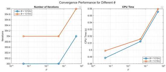
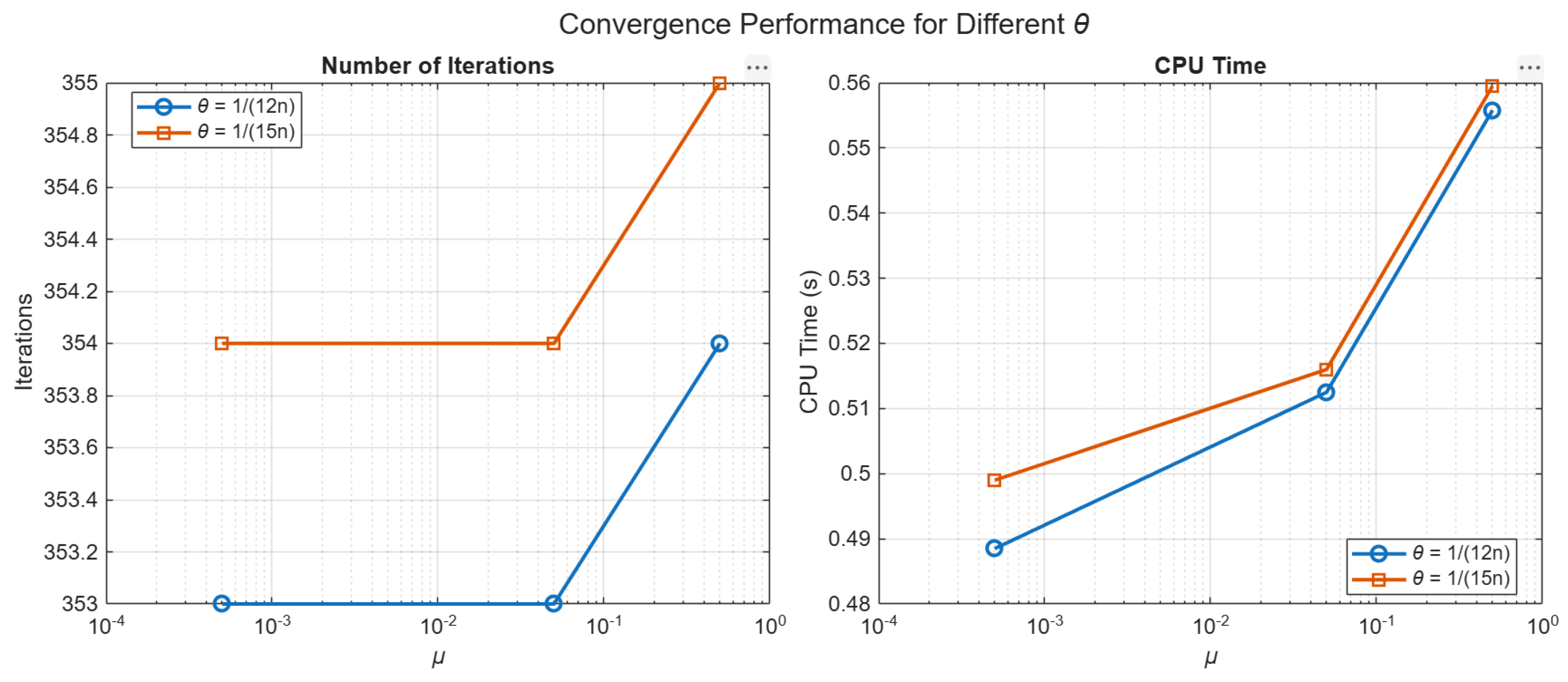
Figure 1. Iterations and CPU time vs. $\mu$ for $\theta ={\displaystyle \frac{1}{12n}}\mathrm{and}\theta ={\displaystyle \frac{1}{15n}}$ for Problem 1.

Problem 2.

For the monotone SDLCP, the Sylvester operator $\mathcal{L}:{\mathbb{S}}^n⟶{\mathbb{S}}^n$ and matrix $Q\in {\mathbb{S}}^n$ are described by:

$$\mathcal{L}\left(X\right)=AX{A}^T+BX{B}^T,$$

with

$$A=\left[\begin{array}{cccccc}1& 2& 0& \cdots & 0& 0\\ 2& 1& 2& \ddots & & ⋮\\ 0& 2& 1& \ddots & \ddots & 0\\ ⋮& \ddots & \ddots & \ddots & 2& 0\\ 0& & \ddots & 2& 1& 2\\ 0& \cdots & 0& 0& 2& 1\end{array}\right],B=\left[\begin{array}{cccccc}4& 0& 0& \cdots & 0& 0\\ 0& 4& 0& \ddots & & ⋮\\ 0& 0& 4& \ddots & \ddots & 0\\ ⋮& \ddots & \ddots & \ddots & 0& 0\\ 0& & \ddots & 0& 4& 0\\ 0& \cdots & 0& 0& 0& 4\end{array}\right]$$

and

$$Q=\left[\begin{array}{cccccc}{\displaystyle \frac{1}{2}}& 0& 0& \cdots & 0& 0\\ 0& {\displaystyle \frac{1}{2}}& 0& \ddots & & ⋮\\ 0& 0& {\displaystyle \frac{1}{2}}& \ddots & \ddots & 0\\ ⋮& \ddots & \ddots & \ddots & 0& 0\\ 0& & \ddots & 0& {\displaystyle \frac{1}{2}}& 0\\ 0& \cdots & 0& 0& 0& {\displaystyle \frac{1}{2}}\end{array}\right]$$

The optimal solution $X^{\ast }\in {\mathbb{S}}_{+}^5$ is given by:

$$X^{\ast }=1.0e-09\times \left[\begin{array}{ccccc}0.1192& -0.0000& -0.0000& -0.0000& -0.0000\\ -0.0000& 0.1192& -0.0000& -0.0000& -0.0000\\ -0.0000& -0.0000& 0.1192& -0.0000& -0.0000\\ -0.0000& -0.0000& -0.0000& 0.1192& -0.0000\\ -0.0000& -0.0000& -0.0000& -0.0000& 0.1192\end{array}\right].$$

The numerical results corresponding to this example, using a feasible initial point $X^0$, are summarized below:

$$X^0=\mathrm{Diag}[1,\dots ,1].$$

Table 2 shows some values of n.

Table 2. Computational results for Problem 2.

$\mathit{\mu }$	$0.5$	$0.05$	$0.005$
	Iter   CPU	Iter   CPU	Iter   CPU
$n=5$	$22483.0478$	$22433.0032$	$22422.9628$
$n=10$	$226019.2116$	$225519.1977$	$225419.1725$
$n=14$	$2259120.8628$	$225493.0687$	$225392.4859$

Problem 3.

For the monotone SDLCP, the symmetric Kronecker sum operator $\mathcal{L}:{\mathbb{S}}^n⟶{\mathbb{S}}^n$ and matrix $Q\in {\mathbb{S}}^n$ are described by:

$$\mathcal{L}\left(X\right)=AX+X{A}^T,$$

where $A\in {\mathbb{R}}^{n\times n}$ and $X\in {\mathbb{S}}^n$. This operator is commonly associated with Lyapunov-type matrix equations. Using the vectorization operator, it can equivalently be expressed as

$$\mathrm{vec}\left(\mathcal{L}\left(X\right)\right)=(I_n\otimes A+A\otimes I_n)\mathrm{vec}\left(X\right),$$

where ⊗ denotes the Kronecker product and $I_n$ is the $n\times n$ identity matrix. Thus, the operator is represented by the Kronecker sum $I_n\otimes A+A\otimes I_n$. In this example, the matrix A is specified below to define the operator used in the numerical experiment:

$$A=\left[\begin{array}{cccccc}3& 1& 0& \cdots & 0& 0\\ 1& 3& 1& \ddots & & ⋮\\ 0& 1& 3& \ddots & \ddots & 0\\ ⋮& \ddots & \ddots & \ddots & 2& 0\\ 0& & \ddots & 1& 3& 1\\ 0& \cdots & 0& 0& 1& 3\end{array}\right],B=\left[\begin{array}{cccccc}2& 0& 0& \cdots & 0& 0\\ 0& 2& 0& \ddots & & ⋮\\ 0& 0& 2& \ddots & \ddots & 0\\ ⋮& \ddots & \ddots & \ddots & 0& 0\\ 0& & \ddots & 0& 2& 0\\ 0& \cdots & 0& 0& 0& 2\end{array}\right]$$

and

$$Q=A^T\ast B=\left[\begin{array}{cccccc}6& 2& 0& \cdots & 0& 0\\ 2& 6& 2& \ddots & & ⋮\\ 0& 2& 6& \ddots & \ddots & 0\\ ⋮& \ddots & \ddots & \ddots & 0& 0\\ 0& & \ddots & 2& 6& 2\\ 0& \cdots & 0& 0& 2& 6\end{array}\right]$$

The optimal solution $X^{\ast }\in {\mathbb{S}}_{+}^5$ is given by

$$X^{\ast }={10}^{-9}\times \left[\begin{array}{ccccc}0.3861& -0.1522& 0.0580& -0.0218& 0.0073\\ -0.1531& 0.4411& -0.1742& 0.0653& -0.0218\\ 0.0582& -0.1743& 0.4479& -0.1743& 0.0582\\ -0.0218& 0.0653& -0.1742& 0.4411& -0.1531\\ 0.0073& -0.0218& 0.0580& -0.1522& 0.3861\end{array}\right].$$

The numerical results corresponding to this example, using a feasible initial point $X^0$, are summarized below:

$$X^0=\mathrm{Diag}[1,\dots ,1].$$

Table 3 shows some values of n.

Table 3. Computational results for Problem 3.

$\mathit{\mu }$	$0.5$	$0.05$	$0.005$
	Iter   CPU	Iter   CPU	Iter   CPU
$n=5$	$17401.9370$	$17361.8809$	$17351.8680$
$n=10$	$176219.3286$	$175715.7241$	$175715.0622$

To further assess solution accuracy, Table 4 reports the terminal feasibility and complementarity errors, the minimum eigenvalues of X and Y, and the final values of $\mu$.

Table 4. Terminal accuracy of the computed solutions.

	${\mathit{e}}_{\mathit{f}}={\parallel {\mathit{R}}_{\mathit{p}}\parallel }_{\mathit{F}}$	$\mathrm{Tr}\left(\mathit{XY}\right)$	${\mathit{\lambda }}_{\min }\left(\mathit{X}\right)$	${\mathit{\lambda }}_{\min }\left(\mathit{Y}\right)$	Final $\mathit{\mu }$
$Pb1$	$9.4763\times {10}^{-9}$	$2.7266\times {10}^{-9}$	0.0582	$1.4350\times {10}^{-9}$	$5.4531\times {10}^{-10}$
$Pb2$	$1.1540\times {10}^{-8}$	$2.9823\times {10}^{-10}$	$1.1929\times {10}^{-10}$	0.5	$5.9647\times {10}^{-11}$
$Pb3$	$1.1593\times {10}^{-9}$	$9.9983\times {10}^{-9}$	$2.0492\times {10}^{-10}$	2.5359	$1.9997\times {10}^{-9}$

Problem 4

(Example: Transformation from CQSDO to SDLCP [24]). We consider the following Convex Quadratic Semi-definite Optimization Problem (CQSDO):

$$\left\{\begin{array}{c}\min C•X+{\displaystyle \frac{1}{2}}X•Q\left(X\right)\hfill \\ \mathit{subject}\mathit{to}{A}_i•X=b_i,\mathrm{for}i=1,\dots ,m\hfill \\ X⪰0\hfill \end{array}\right.$$

where $X\in {\mathbb{S}}^3$, and the linear operator $Q\left(X\right)=HXH$ is defined using:

$$H=\left[\begin{array}{ccc}\sqrt{2}& 0& 0\\ 0& \sqrt{2}& 0\\ 0& 0& 0\end{array}\right],A_1=\left[\begin{array}{ccc}-1& 0& 0\\ 0& 1& 0\\ 0& 0& 0\end{array}\right],A_2=I_3=\left[\begin{array}{ccc}1& 0& 0\\ 0& 1& 0\\ 0& 0& 1\end{array}\right],$$

$$C=\left[\begin{array}{ccc}-2& 0& 0\\ 0& -4& 0\\ 0& 0& 0\end{array}\right],\mathrm{and}b=\left[\begin{array}{c}1\\ 2\end{array}\right].$$

We use the following initial points:

$$X_0=\left[\begin{array}{ccc}0.4& 0& 0\\ 0& 1.4& 0\\ 0& 0& 0.2\end{array}\right],Y_0=\left[\begin{array}{ccc}0.3& 0& 0\\ 0& 0.3& 0\\ 0& 0& 1.5\end{array}\right]$$

Transformation to SDLCP

Let us define:

$$Q\left(X\right)=HXH,\mathcal{A}\left(X\right)=\left(\begin{array}{c}⟨A_1,X⟩\\ ⟨A_2,X⟩\end{array}\right).$$

The optimality condition of the CQSDO problem gives a system:

$$\begin{array}{cc}\hfill HXH+C-{\mathcal{A}}^{\ast }\left(y\right)& =Y,\hfill \\ \hfill \mathcal{A}\left(X\right)& =b,\hfill \\ \hfill X& ⪰0,Y⪰0,XY=0.\hfill \end{array}$$

Let us denote the operator $L\left(X\right)=HXH$ and define:

$$F(X,y)=L\left(X\right)+C-{\mathcal{A}}^{\ast }\left(y\right).$$

Then, the problem is equivalent to the following Semi-definite Linear Complementarity Problem:

$$\mathit{Find}X,Y\in {\mathbb{S}}_{+}^3,\mathit{such}\mathit{that}$$

$$\begin{array}{cc}\hfill & Y=L\left(X\right)+C-{\mathcal{A}}^{\ast }\left(y\right),\hfill \\ \hfill & X⪰0,Y⪰0,X•Y=0.\hfill \end{array}$$

The optimal solution $X^{\ast }\in {\mathbb{S}}_{+}^3$ is given by:

$$X^{\ast }=\left[\begin{array}{ccc}0.5& 0& 0\\ 0& 1.5& 0\\ 0& 0& 0\end{array}\right],$$

The numerical results corresponding to this example, using a feasible initial point $X^0$, are summarized below:

$$X_0=\left[\begin{array}{ccc}1& 0& 0\\ 0& 1& 0\\ 0& 0& 1\end{array}\right],$$

Table 5 shows some values of $\mu$.

Table 5. Computational results for Problem 4.

$\mathit{\mu }$	$0.5$	$0.05$	$0.005$	$0.0005$
Iter	1921	1916	1916	1916
CPU	$0.6275$	$0.5645$	$0.5443$	$0.4669$

Problem 5

(Example: Transformation from SDO to SDLCP). Consider the Semi-definite Program:

$$\begin{array}{c}\hfill \left\{\begin{array}{cc}\underset{X\in {\mathbb{S}}^3}{\min }\hfill & ⟨C,X⟩\hfill \\ \mathrm{s}.\mathrm{t}.\hfill & ⟨A_i,X⟩=b_{i}i=1,\dots ,m,\hfill \\ \hfill & X⪰0,\hfill \end{array}\right.\end{array}$$

(38)

The associated KKT conditions are:

$$\left\{\begin{array}{c}\mathcal{A}\left(X\right)=b,\hfill \\ Y=C-{\mathcal{A}}^{\ast }\left(y\right),\hfill \\ X⪰0,Y⪰0,X•Y=0.\hfill \end{array}\right.$$

where:

$$A_1=\left[\begin{array}{ccccc}0& 1& 0& 0& 0\\ 1& 2& 0& 0& -1\\ 0& 0& 0& 0& 1\\ 0& 0& 0& -2& -1\\ 0& -1& 1& -1& -2\end{array}\right],A_2=\left[\begin{array}{ccccc}0& 0& -2& 2& 0\\ 0& 2& 1& 0& 2\\ -2& 1& -2& 0& 1\\ 2& 0& 0& 0& 0\\ 0& 2& 1& 0& 2\end{array}\right],A_3=\left[\begin{array}{ccccc}2& 2& -1& -1& 1\\ 2& 0& 2& 1& 1\\ -1& 2& 0& 1& 0\\ -1& 1& 1& -2& 0\\ 1& 1& 0& 0& -2\end{array}\right]$$

$$C=\left[\begin{array}{ccccc}3& 3& -3& 1& 1\\ 3& 5& 3& 1& 2\\ -3& 3& -1& 1& 2\\ 1& 1& 1& -3& -1\\ 1& 2& 2& -1& -1\end{array}\right],\mathit{and}b=\left[\begin{array}{c}1\\ 1\\ 1\end{array}\right]$$

Transformation to SDLCP

The system (38) defines a Semi-definite Linear Complementarity Problem:

$$\left\{\begin{array}{c}\mathit{Find}(X,Y)\in {\mathbb{S}}^n\times {\mathbb{S}}^n\hfill \\ \mathit{such}\mathit{that}X⪰0,Y⪰0,\hfill \\ Y=F(X,y),\hfill \\ ⟨A_i,X⟩=b_i,X•Y=0.\hfill \end{array}\right.$$

where:

$$F(X,y)=C-{\mathcal{A}}^{\ast }\left(y\right),{\mathcal{A}}^{\ast }\left(y\right)=y_1{A}_1+y_2{A}_2.$$

The optimal solution $X^{\ast }\in {\mathbb{S}}_{+}^5$ is given by:

$$X^{\ast }=\left[\begin{array}{ccccc}0.0573& 0.1497& 0.0181& 0.0113& 0.0140\\ 0.1497& 0.3909& 0.0473& 0.0296& 0.0366\\ 0.0181& 0.0473& 0.0057& 0.0036& 0.0044\\ 0.0113& 0.0296& 0.0036& 0.0022& 0.0028\\ 0.0140& 0.0366& 0.0044& 0.0028& 0.0034\end{array}\right],$$

The numerical results corresponding to this example, using a feasible initial point $X^0=I_5$, are summarized below (Table 6):

Table 6. Computational results for Problem 5.

$\mathit{\mu }$	$0.5$	$0.05$	$0.005$	$0.0005$
Iter	1442	1437	1437	1437
CPU	$1.9859$	$1.9031$	$1.8206$	$1.6993$

Remark 1.

The numerical results in Table 2, Table 3, Table 4, Table 5 and Table 6 show that the proposed algorithm maintains a relatively stable number of iterations as the barrier parameter μ decreases from $0.5$ to $0.005$. Meanwhile, the CPU time generally exhibits a slight decrease. These observations indicate that the algorithm demonstrates stable numerical behavior for the tested values of μ. For consistency, the comparison with the reference algorithm in Table 7 is conducted using $\mu =0.5$ for both methods.

Table 7. Comparison of the number of iterations and CPU time between the proposed algorithm and Algorithm 2 from [25] for five SDLCP test problems with ($\mu =0.5$).

Example	Iter	CPU Time (s)
Example 1	354 (Algorithm 1)	0.5559
	1744 (Algorithm 2)	0.5992
Example 2 ($n=5$)	2248 (Algorithm 1)	3.0478
	2263 (Algorithm 2)	3.2862
Example 3	1740 (Algorithm 1)	1.9370
	1757 (Algorithm 2)	2.6612
Example 4	1921 (Algorithm 1)	0.6275
	1932 (Algorithm 2)	0.8715
Example 5	1442 (Algorithm 1)	1.9859
	1452 (Algorithm 2)	2.3667

6.2. Comparison Study

Table 7 summarizes the computational performance comparison between the two algorithms, measured by the number of iterations and CPU time required to achieve convergence. The first method, Algorithm 2 from [25], when applied to the SDLCP, exhibited a higher iteration count and marginally longer computation times across all test instances. In contrast, our proposed Algorithm 1 which avoids centering steps and adopts a streamlined infeasible interior-point framework, achieved superior computational efficiency. It consistently converged using fewer iterations and less CPU time. These findings confirm that the proposed algorithm not only maintains the theoretical convergence guarantees but also delivers tangible practical advantages in terms of speed and robustness, making it a compelling choice for solving semi-definite linear complementarity problems (with $ϵ={10}^{-8}$ and ${\mu }_0=0.5$).

7. Conclusions and Future Works

In this paper, we introduced an enhanced version of the classical infeasible interior-point algorithm originally proposed by Mansouri et al. [22] for solving semi-definite linear complementarity problems. The key improvement of our method lies in the removal of centering steps from each main iteration, resulting in a simpler and more computationally efficient approach. We have rigorously shown that the proposed algorithm is well defined and globally convergent. Furthermore, we proved that its iteration complexity achieves the best-known theoretical bound for infeasible interior-point methods in the context of SDLCPs. Extensive numerical experiments demonstrated the superior performance of the proposed algorithm, particularly when employing the newly introduced parameter $\theta ={\displaystyle \frac{1}{12n}}$, which outperformed the parameter choice in [26]. The comparative analysis further revealed that our method consistently requires fewer iterations and less CPU time than the reference algorithm, underscoring its efficiency and practical applicability for solving SDLCPs. For future research, we aim to extend the evaluation of the algorithm to larger-scale and more diverse problem instances to further assess its scalability and real-world performance.

References

- Bai, Y.Q.; El Ghami, M.; Roos, C. A Comparative study of kernel functions for primal-dual interior point algorithms in linear optimization. SIAM J. Optim. 2004, 15, 101–128. [Google Scholar] [CrossRef] [Scilit]
- Zhang, M.W. A large-update interior-point algorithm for convex quadratic semi-definite optimization based on a new kernel function. Acta Math. Sin. 2012, 28, 2313–2328. [Google Scholar] [CrossRef] [Scilit]
- Achache, M. A new parameterized kernel function for LO yielding the best known iteration bound for a large-update interior point algorithm. Afr. Mat. 2015, 27, 591–601. [Google Scholar] [CrossRef] [Scilit]
- Chi, X.; Wang, G. A full-Newton step infeasible interior-point method for the special weighted linear complementarity problem. J. Optim. Theory Appl. 2021, 190, 108–129. [Google Scholar] [CrossRef] [Scilit]
- Achache, M.; Tabchouche, N. Complexity analysis and numerical implementation of large-update interior-point methods for SDLCP based on a new parametric barrier kernel function. Optimization 2018, 67, 1211–1230. [Google Scholar] [CrossRef] [Scilit]
- Achache, M.; Tabchouche, N. A full Nesterov-Todd step primal-dual path-following interior point algorithm for semidefinite linear complementarity problems. CRORR J. 2018, 9, 37–50. [Google Scholar] [CrossRef] [Scilit]
- Chen, F. Polynomial convergence of primal-dual algorithms for SDLCP based on the M-Z family of directions. Appl. Math. Sci. 2011, 5, 1903–1907. [Google Scholar]
- Darvay, Z. New interior point algorithms for linear optimization. Adv. Model. Optim. 2003, 5, 51–92. [Google Scholar]
- Liu, Z.; Sun, W.; Tian, F. A full-Newton step infeasible interior-poit algorithm for linear programming based on a Kernel function. Appl. Math. Optim. 2009, 60, 237–251. [Google Scholar] [CrossRef] [Scilit]
- Wang, C.; Zhu, D. A unified kernel function approach to primal-dual interior-point algorithms for convex quadratic SDO. Numer. Algorithms 2011, 57, 537–558. [Google Scholar] [CrossRef] [Scilit]
- Helmberg, C.; Rendl, F.; Vanderbei, R.J.; Wolkowicz, H. An interior-point method for semidefinite programming. SIAM J. Optim. 1996, 6, 342–361. [Google Scholar] [CrossRef] [Scilit]
- Kojima, M.; Shindoh, M.; Hara, S. Interior point methods for the monotone semidefinite linear complementarity in symmetric matrices. SIAM J. Optim. 1997, 7, 86–125. [Google Scholar] [CrossRef] [Scilit]
- Nesterov, Y.E.; Todd, M.J. Primal-dual interior-point methods for self-scaled cones. SIAM J. Optim. 1998, 8, 324–364. [Google Scholar] [CrossRef] [Scilit]
- Tseng, P. Search directions and convergence analysis of some infeasible path-following methods for the monotone semi-definite LCP. J. Optim. Methods Softw. 1998, 59, 245–268. [Google Scholar] [CrossRef] [Scilit]
- Lustig, I.J. Feasible issues in a primal-dual interior point method for linear programming. Math. Program. 1990, 49, 145–162. [Google Scholar] [CrossRef] [Scilit]
- Zhang, Y. On extending some primal-dual interior-point algorithms from linear programming to semidefinite programming. SIAM J. Optim. 1998, 8, 365–386. [Google Scholar] [CrossRef] [Scilit]
- Guerdouh, S.; Chikouche, W.; Kheirfam, B. A full-Newton step infeasible interior-point algorithm based on a kernel function with a new barrier term. J. Appl. Math. Comput. 2023, 69, 2935–2953. [Google Scholar] [CrossRef] [Scilit]
- Lee, J.K.; Ch, Y.Y.; Jin, J.H.; Cho, G.M. A New full-newton step infeasible interior-point method for P∗(κ)-linear Complementarity problem. Optim. Lett. 2024, 18, 943–964. [Google Scholar] [CrossRef] [Scilit]
- Horn, R.A.; Johnson, C.R. Topics in Matrix Analysis; Cambridge University Press: Cambridge, UK, 1991. [Google Scholar]
- Wang, G.Q.; Bai, Y.Q.; Roos, C. Primal-dual interior-point algorithms for semidefinite optimization based on a simple kernel function. J. Math. Model. Algorithms 2005, 4, 409–433. [Google Scholar] [CrossRef] [Scilit]
- De Klerk, E. Aspects of Semidefinite Programming: Interior Point Methods and Selected Applications; Kluwer Academic Publishers: Dordrecht, The Netherlands, 2002. [Google Scholar]
- Mansouri, H.; Roos, C. A new full-Newton step O(n) infeasible interior-point algorithm for semidefinite optimization. J. Numer. Algorithms 2009, 52, 225–255. [Google Scholar] [CrossRef] [Scilit][Green Version]
- Gowda, M.S.; Song, Y. On semidefinite linear complementarity problem. Math. Program. Ser. A 2000, 88, 575–587. [Google Scholar] [CrossRef] [Scilit]
- Zaoui, B.; Benterki, D.; Adnan, Y. An efficient primal-dual interior point algorithm for convex quadratic semidefinite optimization. J. Appl. Math. Comput. 2024, 70, 2129–2148. [Google Scholar] [CrossRef] [Scilit]
- Bendaas, Y.; Achache, M. A numerical study of an infeasible interior-point algorithm for convex quadratic semi-definite optimization. J. Numer. Anal. Approx. Theory 2024, 53, 199–217. [Google Scholar] [CrossRef] [Scilit]
- Pirhaji, M.; Mansouri, H.; Zangiabadi, M. A full NT-step infeasible interior-point algorithm for semidefinite optimization. RAIRO-Oper. Res. 2017, 51, 533–545. [Google Scholar] [CrossRef] [Scilit]
Disclaimer/Publisher’s Note: The statements, opinions and data contained in all publications are solely those of the individual author(s) and contributor(s) and not of MDPI and/or the editor(s). MDPI and/or the editor(s) disclaim responsibility for any injury to people or property resulting from any ideas, methods, instructions or products referred to in the content. |
© 2026 by the authors. Licensee MDPI, Basel, Switzerland. This article is an open access article distributed under the terms and conditions of the Creative Commons Attribution (CC BY) license.