


Abstract
Accurate and efficient fish detection in underwater environments is fundamental to the advancement of automated aquaculture monitoring and selective fishing systems. However, the deployment of existing object detection models in such environments remains challenging due to wavelength-dependent light absorption, suspended-particle scattering, low contrast, and biological occlusion caused by schooling behavior, all of which are further compounded by the substantial computational overhead of conventional architectures. To address these limitations, this paper proposes FishMonitorAI, a lightweight object detection model built upon the YOLO11n framework and specifically optimized for underwater fish detection. The proposed model incorporates three architectural enhancements: (i) C3k2-DS, a lightweight backbone block leveraging depthwise separable convolutions to reduce computational complexity while preserving feature representation capacity; (ii) C2f-DS, a lightweight neck module that enables efficient multi-scale feature aggregation; and (iii) DySample, a content-aware dynamic upsampling module that replaces fixed interpolation methods to recover fine-grained spatial details critical for small fish localization. Extensive experiments on the DeepFish dataset demonstrate that FishMonitorAI achieves an mAP@0.5 of 98.2% while requiring 5.9 GFLOPs and 2.462 million parameters, corresponding to reductions of approximately 6.3% in GFLOPs and 4.6% in parameter count relative to the YOLO11n baseline. Direct inference measurements on an NVIDIA GTX 1650 Ti further show an average latency of 40.078 ms per image at a batch size of 1 and an input resolution of 640 × 640 pixels. These results demonstrate a favorable balance between detection performance, model complexity, and inference latency on the evaluated GPU platform. However, because the DeepFish dataset was randomly partitioned rather than split by habitat, images from the same habitat may occur across the training, validation, and test subsets. Therefore, the reported results should be interpreted as performance under the current DeepFish split rather than as evidence of generalization to completely unseen underwater environments. Ablation studies and Grad-CAM visualizations further illustrate the complementary contributions of the proposed modules and elucidate their underlying operational mechanisms. The present study evaluates only single-class fish detection; therefore, downstream tasks such as species recognition, disease diagnosis, individual tracking, biomass estimation, and selective harvesting remain outside the scope of the current experiments. The lightweight design of FishMonitorAI makes it a promising candidate for resource-constrained aquaculture monitoring systems; however, deployment performance on representative embedded platforms remains to be validated.
1. Introduction
Traditional fishing operations remain heavily reliant on manual labor, exposing workers to hazardous conditions while suffering from inherent limitations such as low efficiency, weather dependence, and poor species selectivity, leading to unintended bycatch and severe ecosystem degradation [1,2,3]. The advent of automated fishing and aquaculture monitoring systems [4,5,6,7], integrated with autonomous surface vessels [8,9,10], underwater robotic platforms [11,12], and intelligent vision-based monitoring systems [13,14], has substantially mitigated these limitations by enabling continuous operation, reducing labor dependence, and facilitating selective harvesting [15].
Such systems are capable of accurately and reliably detecting underwater objects. However, the underwater imaging environment poses distinct optical challenges, including wavelength-dependent light absorption, scattering caused by suspended particles, reduced contrast, color distortion, and biological occlusion induced by schooling fish, rendering conventional detection algorithms largely inadequate for real-world requirements [16].
Deep learning-based detectors have achieved superior performance across numerous visual recognition benchmarks [17], and are broadly categorized into two main paradigms: two-stage detectors, like R-CNN [18], Fast R-CNN [19], Faster R-CNN [20], and Mask R-CNN [21], which deliver high accuracy at the expense of substantial computational cost, and one-stage detectors, including the YOLO family [22,23,24,25,26,27,28,29], SSD [30], RetinaNet [31], and DETR [32,33], which offer a favorable trade-off between accuracy and computational efficiency.
Nevertheless, the direct deployment of existing YOLO variants in underwater environments remains constrained by two principal weaknesses: (1) fixed upsampling interpolation operations (e.g., nearest-neighbor, bilinear) are content-agnostic and tend to degrade fine-grained spatial details that are critical for the detection of small fish [34]; and (2) standard convolutions incur considerable parameter and computational overhead, limiting their deployability on resource-constrained embedded platforms [35,36].
To address these challenges, this paper proposes FishMonitorAI, a lightweight object detection model built upon the YOLO11n framework and specifically optimized for fish detection in underwater environments, incorporating three architectural improvements: (1) C3k2-DS, which replaces the standard convolutions in the backbone with depthwise separable convolutions [35] to reduce model complexity while preserving feature extraction capability; (2) C2f-DS, which enhances the feature aggregation block in the neck by employing depthwise separable convolutions to enable more efficient multi-scale feature aggregation; and (3) DySample [34], which substitutes the fixed upsampling operation with a content-aware dynamic resampling module, substantially improving the localization of small fish under degraded imaging conditions. The proposed model is evaluated on the DeepFish dataset [37]. The principal contributions of this paper are summarized as follows:
- We proposed C3k2-DS, a lightweight backbone block that leverages depthwise separable convolutions to reduce model complexity without compromising feature representation capacity. Its reduced computational complexity makes it a potentially suitable component for resource-constrained aquaculture monitoring platforms, including autonomous surface vessels, underwater robotic systems, recirculating aquaculture systems, and cage aquaculture.
- We introduced C2f-DS, a lightweight multi-scale feature-fusion module that replaces the standard C3k2 fusion blocks in the YOLO11n neck. The module combines a C2f-derived aggregation structure with depthwise separable convolutions to reduce computational complexity while preserving effective feature reuse across multiple spatial scales. By enabling robust feature fusion across different spatial resolutions, this block addresses the high variability in fish appearance caused by factors such as species diversity, body orientation, and the complex structural backgrounds of underwater habitats, including seagrass beds, rocky substrates, and coral reefs.
- We integrated DySample as a content-aware upsampling block that substantially enhances the detection accuracy of small fish. This is particularly critical in aquaculture settings, where early-stage juveniles and small forage fish are key indicators of stock health and feeding efficiency. Moreover, fish schooling behavior often results in partial occlusion and overlapping individuals, and these challenges are further exacerbated by low light penetration, light attenuation, and suspended particulate matter in turbid water. The adaptive upsampling capability of DySample enables the model to recover fine-grained spatial details essential for distinguishing individual fish under these visually degraded conditions, thereby providing a lightweight fish-detection component that could potentially support downstream aquaculture applications such as selective harvesting, population estimation, and disease surveillance when combined with additional task-specific modules.
2. Related Works
2.1. YOLO Networks
YOLO (You Only Look Once) [22] approaches object detection as an end-to-end regression problem by dividing the input image into an S × S grid, where each cell is responsible for predicting bounding boxes and confidence scores for objects whose centers fall within it. Inspired by GoogLeNet, the original architecture consists of 24 convolutional layers combined with 2 fully connected layers. YOLOv2 [23] introduced key improvements including Batch Normalization, anchor boxes, direct location prediction, and multi-scale training, while the Darknet-19 backbone reduced computational cost to 5.58 billion operations—substantially lower than VGG-16 [38] and GoogLeNet. YOLOv3 [24] incorporated mechanisms from FPN [39] and ResNet [40], enabling multi-scale predictions at three resolution levels and significantly improving small object detection via the Darknet-53 backbone. YOLOv4 [25] optimized training on a single GPU by integrating CSP connections, CmBN normalization, Mosaic data augmentation, and the Mish activation function, with PANet [41] replacing FPN in the neck for more effective multi-scale feature aggregation. YOLOv5 [42], developed by Ultralytics, inherited the CSP-Darknet53 backbone and enhanced the neck by combining SPP with BottleNeckCSP within the PANet structure, striking a favorable balance between speed and accuracy. YOLOv8 [26] adopted an anchor-free design with a decoupled detection head separating classification, localization, and objectness prediction into three independent branches, improving precision while simplifying the detection pipeline for real-time applications. YOLOv9 [43] introduced Programmable Gradient Information (PGI) to maintain stable gradient flow throughout the network and the Generalized Efficient Layer Aggregation Network (GELAN) for flexible multi-scale feature aggregation, collectively addressing information loss in deep networks and improving detection of small objects. YOLOv10 [27] eliminated the Non-Maximum Suppression (NMS) post-processing step through a dual assignment strategy combining one-to-many and one-to-one label assignment, and further incorporated spatial-channel decoupled downsampling and rank-guided block design to reduce redundancy and optimize parameter utilization. YOLO11 [28,44] replaced the C2f module used in earlier Ultralytics architectures with the C3k2 block in its feature-extraction and feature-fusion stages, while retaining a decoupled Detect head for multi-scale prediction. It also integrates SPPF to enrich multi-scale contextual representation and employs the C2PSA module to refine spatial feature learning, thereby improving detection performance under occlusion and complex backgrounds. Finally, YOLOv12 [29] adopted an attention-centric architecture centered on the Area Attention (A2) module for dynamic receptive field adjustment, complemented by the Residual Efficient Layer Aggregation Network (R-ELAN) for stable gradient-driven feature fusion, alongside Flash Attention and adaptive MLP ratios to further accelerate inference while sustaining high detection accuracy.
2.2. YOLO for Fish Detection
In recent years, the problem of automated fish detection and recognition in underwater environments has attracted growing interest from the research community, with applications spanning marine ecological surveys, ocean geographic studies, and sustainable aquaculture monitoring. Compared to manual identification, which is time-consuming and operationally costly, computer vision-based automated approaches offer considerable potential for improving monitoring efficiency [45,46,47,48]. Nevertheless, the inherent characteristics of underwater environments, including weak and uneven illumination, complex backgrounds, high luminance variation, free movement of fish, and substantial morphological diversity across species, pose significant challenges to the detection accuracy of modern systems. Morphometric studies have further demonstrated that fish species exhibit measurable differences in body shape and proportions, which can contribute to species characterization and identification [49].
Al Muksit et al. [50] proposed YOLO-Fish, a deep learning-based fish detection framework comprising two variants. YOLO-Fish-1 improves upon YOLOv3 by adjusting upsampling step sizes to reduce the miss rate for small-scale individuals. YOLO-Fish-2 further extends this by incorporating an additional Spatial Pyramid Pooling module, enhancing detection capability under dynamic and complex environmental conditions. Both models were evaluated on two benchmark datasets: DeepFish—comprising approximately 15,000 bounding box annotations across 4505 images from 20 distinct habitats—and OzFish—containing approximately 43,000 annotations of multiple fish species over around 1800 images. Experimental results demonstrated that YOLO-Fish-1 and YOLO-Fish-2 achieved mean Average Precision (mAP) of 76.56% and 75.70%, respectively, under unconstrained real-world marine conditions, significantly outperforming the original YOLOv3 while maintaining a lighter model size compared to YOLOv4 at comparable performance levels.
Ouis and Akhloufi [51] presented a study on fish detection in underwater environments using sonar imagery from the Caltech Fish Counting (CFC) dataset. The study optimized and evaluated the performance of YOLOv7 and YOLOv8 on a training set of 162,680 images and a test set of 334,017 images. Results indicated that YOLOv7 achieved AP50 of 68.3% and AP75 of 62.15%, while YOLOv8 surpassed it with AP50 of 72.47% and AP75 of 66.21%, affirming the effectiveness of modern deep learning models under diverse underwater observation conditions and their generalization capacity on large-scale datasets.
Vijayalakshmi and Sasithradevi [52] proposed AquaYOLO, a fish detection architecture specifically optimized for aquaculture pond monitoring. The model’s backbone leverages CSP layers combined with enhanced convolutions to extract hierarchical features, while the neck enriches feature representation through upsampling, concatenation, and multi-scale fusion. The detection head operates at a 40 × 40 resolution and omits the final C2f layer to improve localization precision. The model was evaluated on the DePondFi dataset—encompassing approximately 50,000 bounding box annotations across 8150 images collected from aquaculture ponds in southern India—and achieved a precision of 0.889, recall of 0.848, and mAP@50 of 0.909, demonstrating strong practical applicability in low-cost aquaculture monitoring systems.
Jiang et al. [53] proposed Mobile-YOLO, a lightweight object detection architecture designed specifically for recognizing four aquatic species: sea cucumbers, sea urchins, scallops, and starfish. The model introduces a novel backbone, Mobile-Nano, to strengthen feature extraction while preserving a compact structure, coupled with a lightweight detection head LDtect to balance model compression with detection accuracy. In addition, DySample and HWD (Haar Wavelet Downsampling) modules are incorporated to optimize the upsampling and downsampling processes within the feature fusion structure. Compared to the baseline, Mobile-YOLO reduces parameters by 32.2%, FLOPs by 28.4%, and model size by 30.8%, while improving FPS by 95.2% and increasing mAP by 1.6%. When benchmarked against mainstream models including YOLOv5–12, SSD, EfficientDet, RetinaNet, and RT-DETR, Mobile-YOLO achieves leading performance in both accuracy and compactness, confirming its practical potential for real-time aquatic organism recognition systems.
Lei et al. [54] proposed an integrated aquaculture monitoring system combining a low-cost bionic robotic fish with the YOLO-PWSL underwater fish recognition model, developed in response to severe water pollution causing losses exceeding 4.6 × 10⁷ kg of aquatic products in China. The robotic fish is equipped with a propulsive caudal fin, an adaptive buoyancy control mechanism, and multiple water quality sensors, enabling real-time environmental parameter monitoring. YOLO-PWSL, developed on the YOLOv5s backbone, incorporates three architectural enhancements: the LGFB multi-level attention fusion module to improve perception under complex conditions, the Wise-ShapeIoU loss function to optimize bounding box localization accuracy, and the lightweight PConv convolution to reduce computational overhead. Experimental results show that the model achieves mAP@0.5 of 96.1%, while reducing parameters by 1.8 million and FLOPs by 3.1 GFLOPs compared to the baseline, with significantly improved miss detection rates, affirming its deployment potential in intelligent aquaculture monitoring systems.
Van Nghia et al. [55,56] proposed a diseased fish detection and counting system based on an enhanced YOLO11 architecture, targeting application in intelligent aquatic robots. The research is motivated by the critical operational reality in high-density aquaculture systems, where disease outbreaks can spread rapidly and cause severe economic losses if not detected in a timely manner. The model was trained and evaluated on a two-class dataset (diseased/healthy fish) with manual annotations, achieving mAP@0.5 of 98.2%, mAP@0.5:0.95 of 76.9%, precision of 96.4%, and recall of 95.2%. The system meets real-time processing requirements, enabling early identification of fish skin pathologies for prompt intervention, thereby mitigating the risk of widespread disease outbreaks and opening a promising research direction for next-generation intelligent aquaculture systems.
3. Materials and Methods
3.1. Overall Architecture of the FishMonitorAI Model
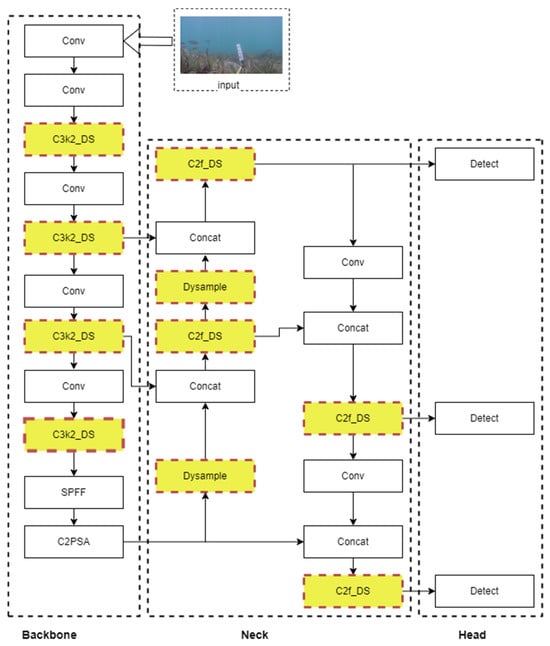
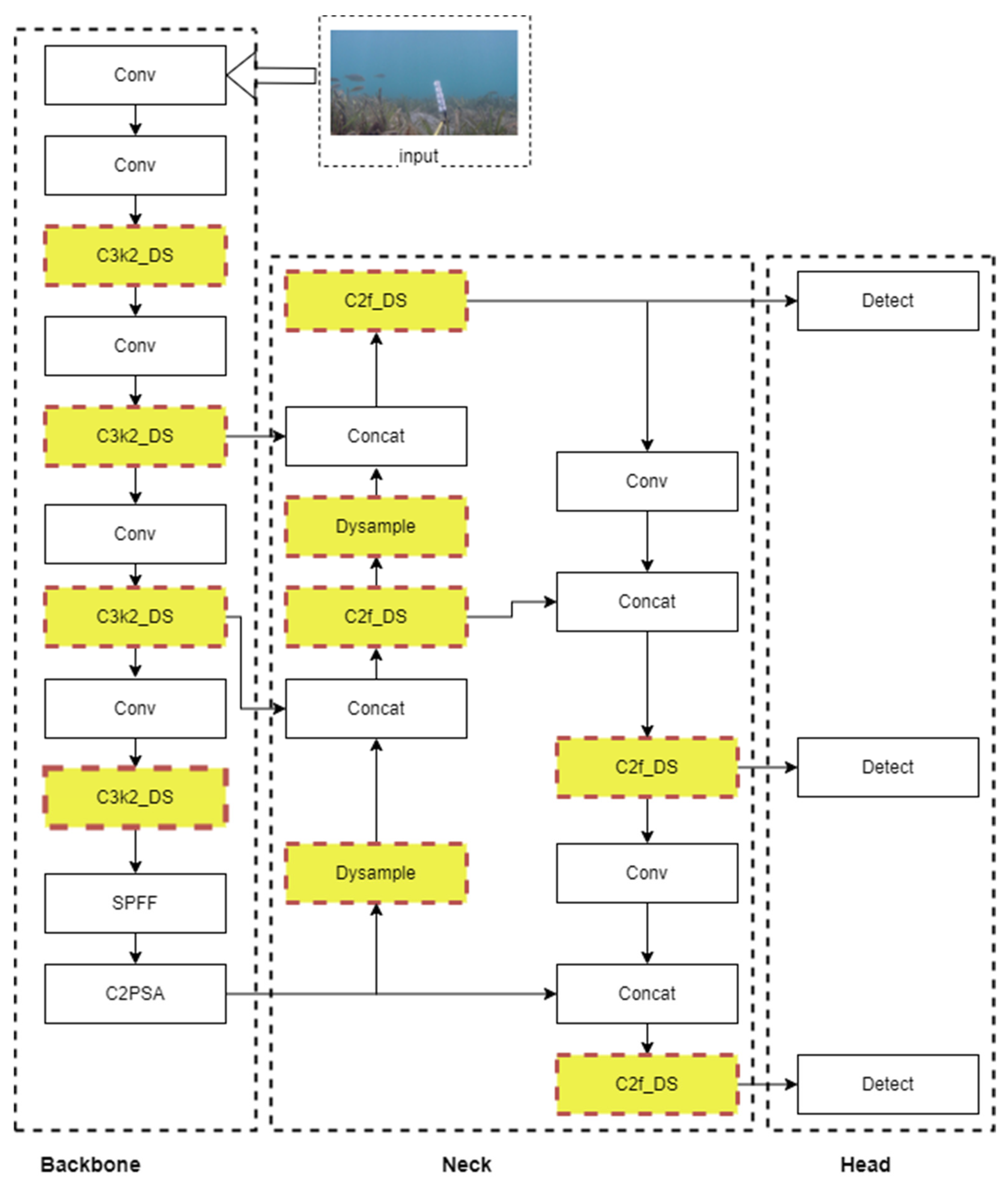
FishMonitorAI is proposed as a lightweight yet high-accuracy object detection model specifically designed for fish detection in complex aquatic environments, where targets are typically small, morphologically diverse, and subject to significant background noise and challenging illumination conditions. Built upon the YOLO11n baseline, the proposed architecture introduces three targeted modifications—C3k2-DS, C2f-DS, and DySample—systematically applied across the backbone and neck, while retaining the original Detect head. The overall network architecture is illustrated in Figure 1, where the modified modules are highlighted in yellow with red dashed borders.
Figure 1.
Overall architecture of FishMonitorAI. Modified modules are highlighted in yellow with red dashed borders. C3k2-DS is introduced in the backbone, while C2f-DS and DySample are incorporated into the neck; the Detect head remains unchanged.
The backbone of FishMonitorAI retains the overall hierarchical structure of YOLO11n. The selected standard C3k2 feature-extraction blocks are replaced with the proposed C3k2-DS modules, in which depthwise separable convolutions are introduced to reduce computational complexity while preserving feature representation capacity. The subsequent SPPF and C2PSA modules are retained from the original YOLO11n architecture. Each C3k2-DS block employs Depthwise Separable Convolutions in place of standard convolutions (Section 3.2).
The neck architecture adopts a top-down feature pyramid structure responsible for multi-scale feature fusion across different semantic levels. Two key modifications are introduced in this component. First, the standard nearest-neighbor upsampling layers are replaced with DySample, a content-aware dynamic upsampler that generates adaptive sampling coordinates from the input feature representations, enabling more faithful spatial detail recovery during feature map upscaling. Second, the standard C3k2 feature-fusion blocks in the YOLO11n neck are replaced with the proposed C2f-DS modules (Section 3.3). This modification therefore constitutes a C3k2-to-C2f-DS architectural substitution rather than a simple C2f-to-C2f-DS replacement. The neck produces three feature maps at different spatial resolutions, which are subsequently forwarded to the unchanged detection head.
In the head the original decoupled Detect module of YOLO11n is retained without structural modification. The three feature maps generated by the modified neck are directly fed into the Detect module for classification and bounding-box regression. This configuration enables the model to simultaneously perform accurate localization and classification across small, medium, and large fish instances within a single forward pass.
Through the combined integration of C3k2-DS in the backbone and C2f-DS and DySample in the neck, FishMonitorAI aims to improve the balance between model complexity and detection performance while retaining the original YOLO11n Detect head.
3.2. Description of New Block C3k2-DS
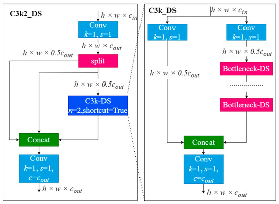
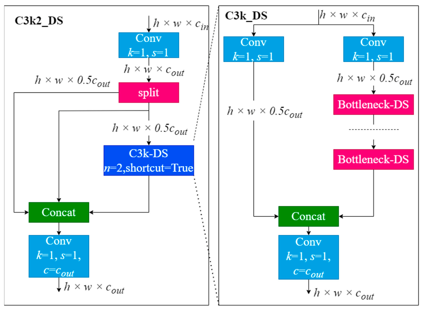
The C3k2-DS block is introduced as a lightweight modification of the standard C3k2 feature extraction module [26], in which all conventional convolutional operations are replaced with Depthwise Separable Convolutions (DSConv) [35]. The architectural design of C3k2-DS is illustrated in Figure 2.
Figure 2.
Architecture of the proposed C3k2-DS feature extraction block.
Formally, given an input tensor of dimensions , the C3k2-DS block sequentially executes four operations. First, a pointwise projection convolution reduces the input to . The resulting tensor is then partitioned along the channel axis into two equal branches of dimensions . The first branch serves as a direct skip connection [43], transmitting low-level spatial information unaltered to the aggregation stage. The second branch is processed through a C3k-DS sub-block with stacked Bottleneck-DS layers and residual shortcut connections enabled [43], enabling hierarchical extraction of multi-scale spatial features. The outputs of both branches are subsequently fused via channel-wise concatenation, and a final pointwise convolution projects the aggregated representation into the output tensor of dimensions .
The C3k-DS sub-block embedded within C3k2-DS constitutes a further lightweight adaptation of the standard C3k module [26]. Rather than employing a channel-splitting strategy as in C3k2-DS, C3k-DS processes the input tensor through two parallel branches, each performing an independent pointwise projection to reduce the channel dimensionality to . The left branch propagates directly to the concatenation stage as a skip connection, while the right branch traverses sequentially stacked Bottleneck-DS blocks [35,36] to perform deep hierarchical spatial feature extraction. The dual-branch outputs are merged via channel-wise concatenation, followed by a final pointwise convolution to yield the output tensor . Unlike C3k2-DS, C3k-DS omits the explicit channel-splitting operation and instead relies on parallel dual projections, providing more granular extraction of high-level semantic representations while preserving the computational advantages conferred by depthwise separable convolutions relative to the original C3k formulation.
By systematically replacing standard convolutions with their depthwise separable counterparts throughout both C3k2-DS and C3k-DS, the proposed modifications achieve meaningful reductions in model parameters and computational complexity [35,57] compared to their standard counterparts, while retaining sufficient feature expressiveness for accurate fish detection.
3.3. Description of New Block C2f-DS
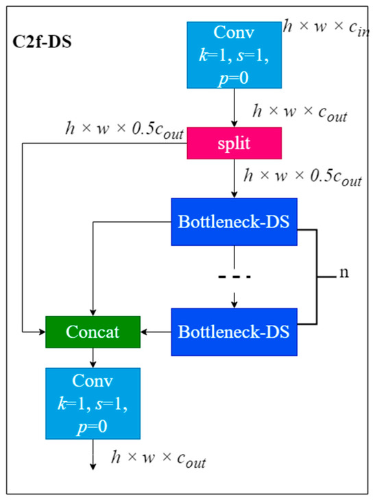
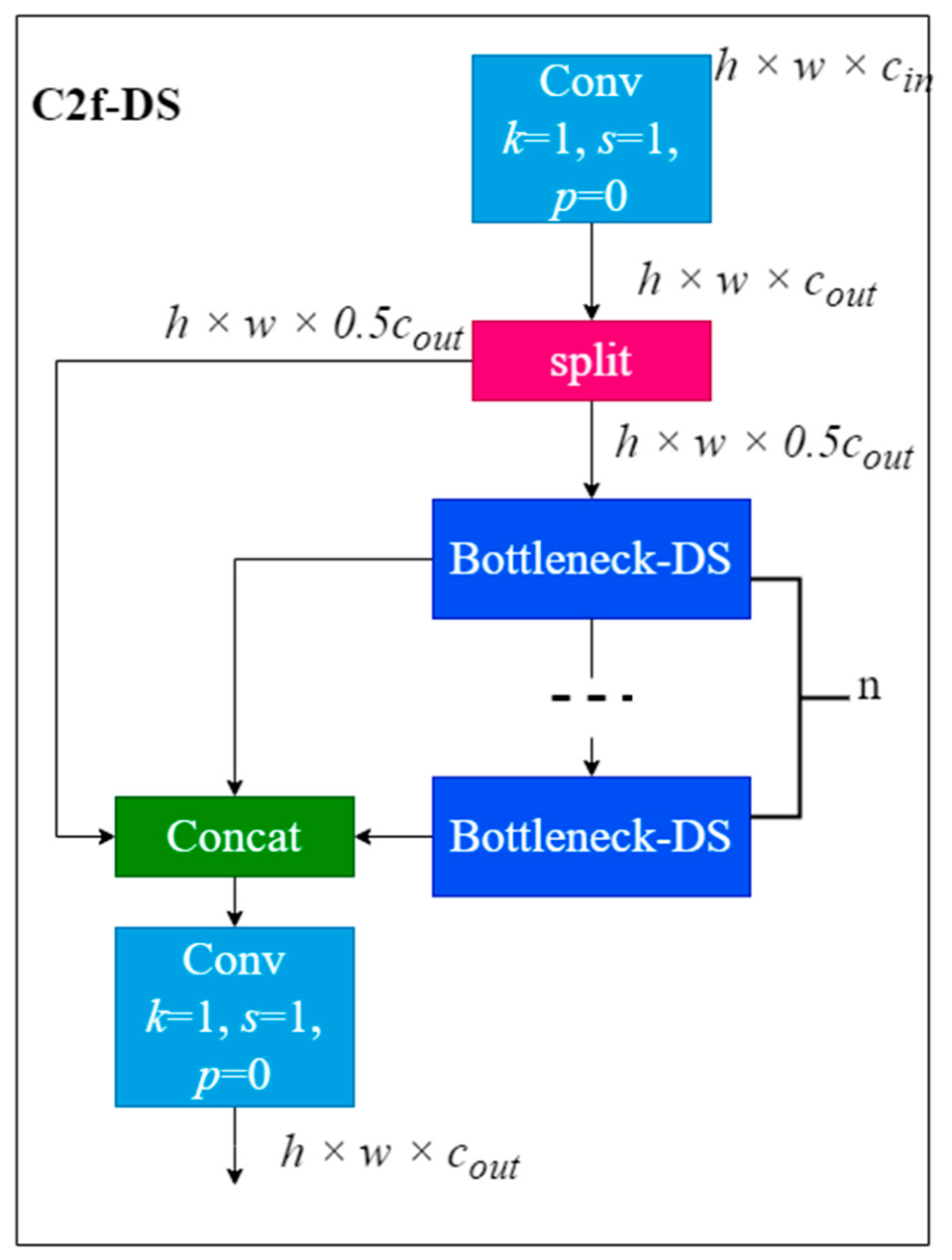
Analogous to C3k2-DS (Section 3.2), C2f-DS applies DSConv [35] within the Bottleneck sub-blocks, but is derived from the standard C2f module [26] rather than C3k2. The architectural design of C2f-DS is illustrated in Figure 3. It should be emphasized that the corresponding feature-fusion stages in the original YOLO11n architecture employ C3k2 blocks rather than C2f blocks. Therefore, the use of C2f-DS in FishMonitorAI constitutes a deliberate architectural substitution of C3k2 with a C2f-derived lightweight aggregation structure. This design combines dense reuse of intermediate features through channel-wise concatenation with reduced computational complexity achieved by depthwise separable convolutions. Consequently, the effect of C2f-DS should be attributed to both the modified feature-fusion structure and the use of depthwise separable convolution, rather than to depthwise separable convolution alone.
Figure 3.
Architecture of the proposed C2f-DS feature extraction block.
C2f-DS follows the same input-projection and channel-split scheme as C3k2-DS (Section 3.2, Figure 2). The second branch is passed sequentially through stacked Bottleneck-DS blocks, each employing depthwise separable convolutions to progressively extract hierarchical feature representations at increasing levels of abstraction. The outputs of all intermediate Bottleneck-DS blocks, together with the skip connection branch, are subsequently aggregated via channel-wise concatenation. A final pointwise convolution is then applied to fuse the concatenated representations and project them into the output tensor of dimensions .
The key distinction between C2f-DS and its predecessor C3k2-DS lies in the configurable depth parameter , which governs the number of stacked Bottleneck-DS blocks and enables flexible adaptation of the network’s representational capacity to the complexity of the target detection task. This design philosophy aligns with the principle of scalable lightweight architecture, allowing the model to balance between computational efficiency and feature expressiveness without structural redesign. Within FishMonitorAI, the computational effect of C2f-DS results from both the replacement of the original C3k2 fusion structure with a C2f-derived aggregation scheme and the use of depthwise separable convolutions inside its Bottleneck-DS blocks. This combination is intended to reduce computational complexity while retaining effective multi-scale feature aggregation.
3.4. Description of New Block DySample
In object detection networks, the upsampling module plays a critical role in restoring the spatial resolution of feature maps within the neck architecture. Conventional interpolation-based approaches, such as nearest-neighbor and bilinear interpolation, determine sampling kernels solely based on the geometric positions of pixels, entirely disregarding the semantic content embedded within the feature representations. This content-agnostic nature inevitably leads to spatial distortion and local information degradation during the upsampling process. Such limitations become particularly pronounced in small object detection scenarios, where preserving fine-grained spatial details is essential for accurate localization—a challenge that is further amplified in aquatic environments characterized by low illumination and high water turbidity.
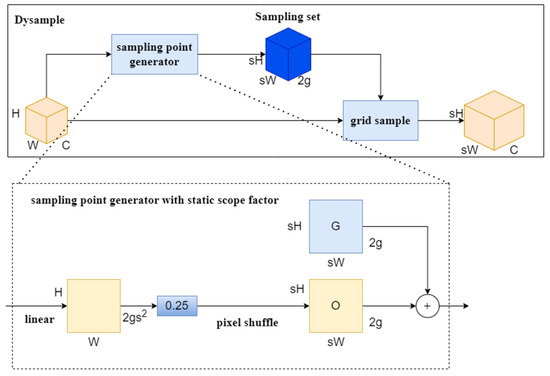
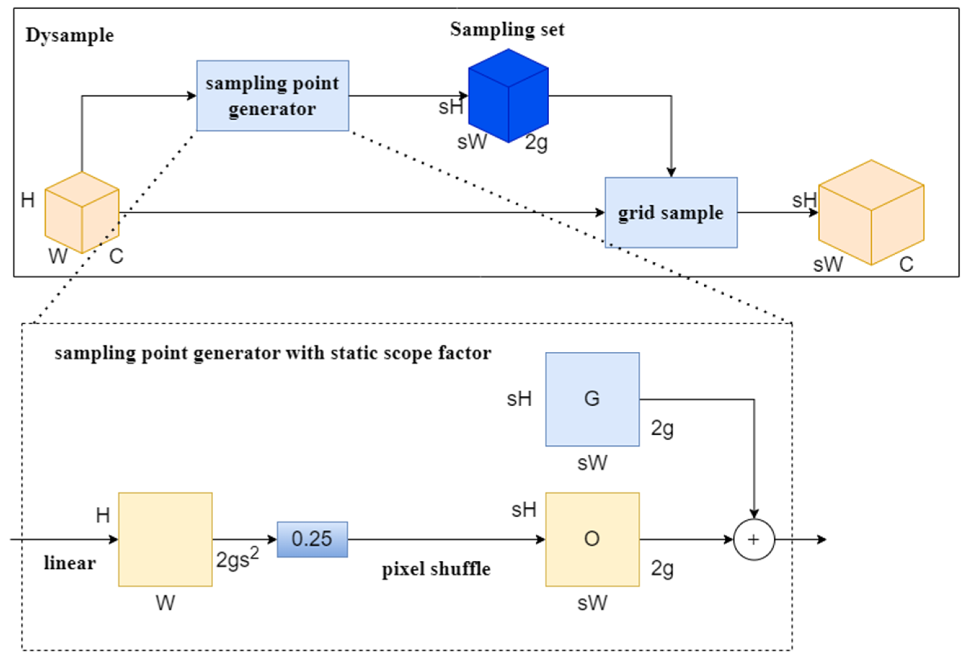
To overcome these limitations, this study incorporates DySample [34]—an ultra-lightweight dynamic upsampler with adaptive spatial reconstruction capability—into the neck architecture of the proposed model, replacing the default interpolation-based upsampling layer. Rather than relying on fixed sampling kernels, DySample dynamically generates content-guided sampling points by learning positional offsets directly from the input feature representations, enabling the production of high-resolution output feature maps with substantially improved spatial fidelity. The overall architecture of DySample is illustrated in Figure 4.
Figure 4.
Network architecture of DySample: sampling point generator with Static Scope Factor modes.
Architecturally, DySample operates through a dynamic point generation mechanism built upon two core components: a base sampling grid and a learned dynamic offset set derived from the input features. Formally, given an input feature map of dimensionality and an upsampling scale factor , the input features are first projected through a linear layer producing output channels:
The resulting offset tensor is subsequently restructured into dimensions via a pixel shuffle operation. The final sampling set is then constructed by superimposing the dynamic offset onto the base sampling grid :
The upsampled output feature map of size is ultimately obtained by resampling the original feature map at the coordinates defined by δ through a grid-based bilinear resampling operation:
This formulation enables the model to concentrate sampling efforts at semantically informative regions rather than uniformly distributing them across spatial positions, as is the case with conventional fixed-kernel methods.
From an efficiency standpoint, DySample distinguishes itself from preceding content-aware upsampling methods such as CARAFE [58] by entirely foregoing the use of kernel prediction sub-networks and dynamic convolution operations. Instead, the sampling offset generation relies exclusively on a lightweight linear projection followed by pixel rearrangement—two computationally inexpensive operations that introduce negligible parameter overhead. This streamlined design facilitates seamless integration into the YOLO11n neck without substantially increasing model complexity, while simultaneously delivering superior spatial feature reconstruction compared to traditional interpolation techniques. These properties are particularly beneficial for detecting small fish instances in complex underwater environments, where input image quality is frequently compromised by adverse visual conditions.
4. Experimental Results
4.1. Datasets
All experiments in this study were conducted using a publicly available object-detection version of the DeepFish dataset [37]. The original underwater images originate from the DeepFish dataset collected across 20 different aquatic habitats in tropical Australia. For the present experiments, we used a processed version in which fish instances had already been annotated with bounding boxes in YOLO-compatible format.
The authors of the present study did not create, modify, or manually refine these bounding-box annotations. The annotation files were obtained together with the processed dataset and were used directly in the experiments. The dataset used in this study contains 4505 images, divided into 3153 training images, 676 validation images, and 676 test images using a random train/validation/test split. Consequently, images originating from the same habitat may occur in different subsets, and the resulting evaluation should not be interpreted as a habitat-disjoint generalization test. This limitation is further discussed in Section 5. The detection task contains a single object class, namely fish. All images were resized to 640 × 640 pixels before being provided to the detection models, while the bounding-box coordinates were represented in the normalized YOLO format. The single-class nature of the dataset is well-aligned with the fish detection objective of this study and eliminates potential class imbalance effects that could otherwise confound performance evaluation.
From a statistical perspective, the dataset presents considerable detection difficulty due to the prevalence of small-sized fish instances, frequent occlusion by aquatic vegetation, and low target-to-background contrast in turbid water conditions. A significant number of annotated instances occupy a small part of the total image area, making DeepFish a challenging benchmark that effectively stress-tests the small object detection capability of the proposed model. These properties collectively justify the selection of DeepFish as the primary evaluation benchmark for FishMonitorAI, as it closely mirrors the operational conditions targeted by the proposed system.
4.2. Evaluation Metrics
To comprehensively evaluate the model’s performance, we employ a multi-dimensional set of metrics covering both detection accuracy and computational efficiency criteria. Regarding detection accuracy, the primary metric used is mean Average Precision at an IoU threshold of 0.5, denoted as mAP@0.5. This metric measures the model’s ability to accurately localize and correctly classify objects across the entire dataset. The IoU threshold of 0.5 was selected because it is the prevailing standard in small object detection tasks, where the small size of bounding boxes makes achieving higher IoU thresholds significantly more difficult. A detection is considered correct when the IoU between the predicted box and the ground truth box reaches at least 0.5. In addition to mAP, we report three supplementary metrics: Precision, Recall, and F1-Score. Specifically, Precision is calculated using the formula , reflecting the proportion of true detections among all positive detections, where a high value indicates that the model produces few false alarms. Recall is calculated using the formula , reflecting the proportion of actual objects that are correctly detected, where a high value indicates that the model misses few objects. F1-Score is calculated using the formula , which is the harmonic mean of Precision and Recall, providing a balanced evaluation between the two metrics, and is particularly meaningful in the context of a dataset containing only a single object class.
Regarding model complexity, two hardware-independent metrics are reported: the number of parameters and the number of floating-point operations, expressed in GFLOPs. The parameter count represents the number of trainable model parameters and provides an indication of model storage and memory requirements. GFLOPs quantify the computational operations required for a forward pass at an input resolution of 640 × 640 pixels and are used as a proxy for computational complexity. For all compared models, parameter counts and GFLOPs were calculated using the same profiling procedure and the same input resolution to ensure a consistent comparison. These metrics characterize theoretical model complexity and should not be interpreted as direct measurements of inference latency or real-time performance, which depend on the target hardware, runtime implementation, precision, and batch size. In addition to these hardware-independent complexity measures, inference latency was directly evaluated to characterize the execution performance of the compared models. The latency benchmark was conducted using the PyTorch 2.6.0 runtime on an NVIDIA GTX 1650 Ti GPU with a batch size of 1 and an input resolution of 640 × 640 pixels. The same numerical precision and inference protocol were used for all compared models. Warm-up iterations were excluded before timing, and the reported latency represents the average over repeated inference runs. Because inference latency is hardware- and runtime-dependent, the reported values characterize execution performance only under the specified experimental configuration and should not be directly generalized to other hardware platforms.
4.3. Implementation Details
All experiments in this study were conducted on the Ubuntu 24.04 LTS operating system using Python 3.12. To ensure a fair comparison and evaluation across all models, the training configuration was kept consistent throughout the experiments. Each model was trained for 300 epochs with an input resolution of 640 × 640 pixels and a batch size of 16. The Stochastic Gradient Descent (SGD) optimizer was employed with a momentum of 0.937 and a weight decay of 5 × 10⁻⁴ to mitigate overfitting. The initial learning rate was set to 0.01 and was adjusted according to a Cosine Annealing schedule throughout training, facilitating more stable convergence in the later stages. To enhance data diversity and improve the generalization capability of the model, several data augmentation techniques were applied during training, including Mosaic, MixUp, HSV color-space adjustment, random horizontal flipping, and random scaling. These augmentation strategies enable the model to learn more diverse feature representations, which is particularly beneficial for detecting small objects such as fish in complex aquatic environments. The complete training configuration and hyperparameter settings are summarized in Table 1.
Table 1.
Training Hyperparameter Configuration.
The same augmentation pipeline (Mosaic, MixUp, HSV color-space adjustment, random horizontal flipping, and random scaling), together with identical hyperparameters and training schedule (300 epochs, SGD optimizer, batch size of 16, Cosine Annealing schedule) as listed in Table 1, was applied uniformly to all compared architectures in Table 2 (YOLOv8n, YOLOv9t, YOLOv10n, YOLO11n, YOLOv12n, and FishMonitorAI), with no model-specific tuning of the augmentation policy or hyperparameters. All reported training results correspond to a single training run per configuration under the same experimental settings. Therefore, small differences between models should be interpreted cautiously, as run-to-run variability was not quantified in the present study. For the inference-time benchmark, all compared architectures were evaluated under identical conditions using a batch size of 1, an input resolution of 640 × 640 pixels, and the same PyTorch runtime and numerical precision. Warm-up iterations were excluded before latency measurement to minimize initialization overhead, and latency was averaged over repeated forward passes.
Table 2.
Comparison of detection performance, computational complexity, and inference latency across YOLO variants.
4.4. Comparative Results
To comprehensively evaluate the effectiveness of FishMonitorAI, we conducted a comparative analysis against several state-of-the-art object detection models, including YOLOv8n, YOLOv9t, YOLOv10n, YOLO11n, and YOLOv12n, on the DEEPFISH dataset. The detailed results are presented in Table 2.
FishMonitorAI achieves an mAP@0.5 of 98.2%, compared with 98.1% for YOLOv8n. However, because the reported values correspond to single training runs and the difference is only 0.1 percentage points, this margin should not be interpreted as statistically significant superiority. Instead, the results indicate that FishMonitorAI provides competitive detection performance while maintaining low computational complexity. FishMonitorAI also attains a Precision of 96.4%, Recall of 95.2%, and F1-score of 95.8%. Importantly, it does not achieve the highest mAP@0.5:0.95: its value of 76.9% is lower than YOLOv8n (77.6%) and YOLOv10n (77.0%). This suggests that the performance advantage observed at IoU = 0.5 does not fully carry over to stricter localization thresholds. One possible explanation is that the proposed architecture improves sensitivity to small, low-contrast, and partially occluded fish, thereby increasing successful detections at a moderate IoU threshold, while small bounding-box localization errors become more strongly penalized at higher IoU thresholds. In terms of computational complexity, FishMonitorAI requires 5.9 GFLOPs, the lowest GFLOP count among the compared models, while maintaining a compact parameter count of 2.462 million. Compared with the YOLO11n baseline, which requires 6.3 GFLOPs and contains 2.582 million parameters, FishMonitorAI reduces computational complexity by approximately 6.3% and the parameter count by approximately 4.6%. Overall, the proposed architecture demonstrates a favorable balance between detection performance and computational efficiency rather than absolute superiority across all evaluation metrics. Direct inference measurements further show that FishMonitorAI achieves the lowest latency among the compared models under the evaluated configuration. FishMonitorAI requires 40.078 ms per image, compared with 43.685 ms for the YOLO11n baseline, corresponding to an approximately 8.3% reduction in inference latency. The remaining models require 46.844 ms (YOLOv8n), 91.758 ms (YOLOv9t), 50.241 ms (YOLOv10n), and 62.912 ms (YOLOv12n). These results demonstrate that, under the evaluated PyTorch/GTX 1650 Ti configuration, the reduction in theoretical computational complexity is accompanied by a measurable reduction in wall-clock inference latency. Nevertheless, these latency values are hardware- and runtime-specific and should not be interpreted as evidence of equivalent performance on embedded platforms.
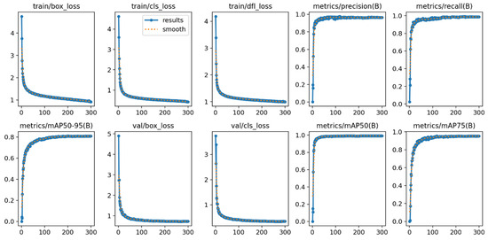
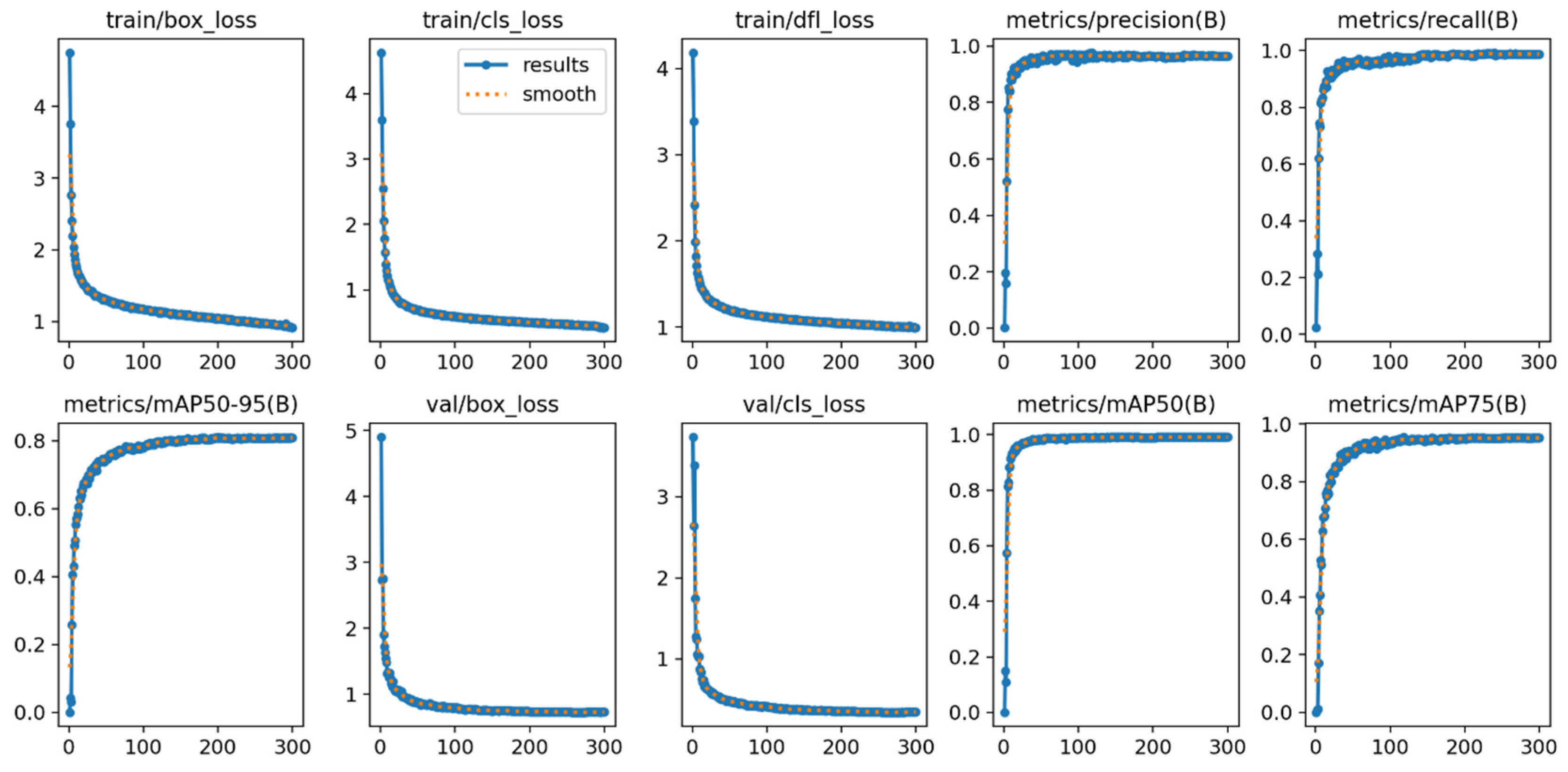
Figure 5 presents an overview of the training process, including three loss components on the training set (box_loss, cls_loss, and dfl_loss), the corresponding three loss components on the validation set, and the validation metrics Precision, Recall, mAP@0.5, mAP@0.75, and mAP@0.5:0.95. Figure 5 therefore reflects model performance on the validation subset during training, whereas the final comparative results reported in Table 2 were obtained on the held-out test subset after training. All models in Table 2 were evaluated on the same test split using the same evaluation protocol and identical confidence and NMS threshold settings.
Figure 5.
Training dynamics of the proposed model over 300 epochs, showing training and validation losses together with validation Precision, Recall, mAP@0.5, mAP@0.75, and mAP@0.5:0.95.
All three loss components decrease rapidly during the first 30 epochs and then continue to decline more gradually before stabilizing, indicating stable optimization without signs of divergence. The training and validation loss curves exhibit similar overall trends, suggesting that the model does not exhibit severe overfitting under the current data split. Precision and Recall increase rapidly during the early stages of training and remain consistently high after convergence. Figure 5 reports validation-set metrics recorded during training, whereas the final comparative results in Table 2 were computed on the held-out test subset after training. The validation curves should therefore not be interpreted as the final test-set performance. Upon convergence, the validation mAP@0.5 approaches approximately 0.99 and the validation mAP@0.5:0.95 reaches approximately 0.81. These values are higher than the corresponding test-set results of 98.2% and 76.9% reported in Table 2, reflecting the expected difference between validation-time monitoring and final evaluation on the held-out test subset. These results indicate stable convergence under the adopted training protocol. However, because the dataset was randomly divided rather than split by habitat, they should not be interpreted as evidence of generalization to completely unseen underwater environments.
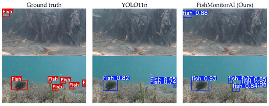
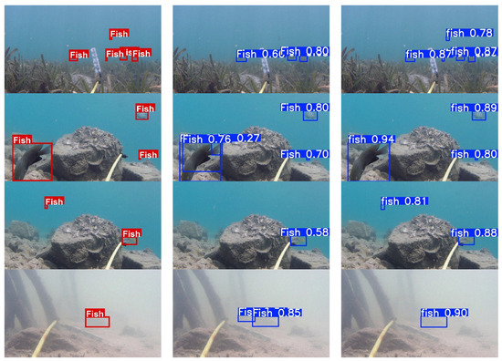
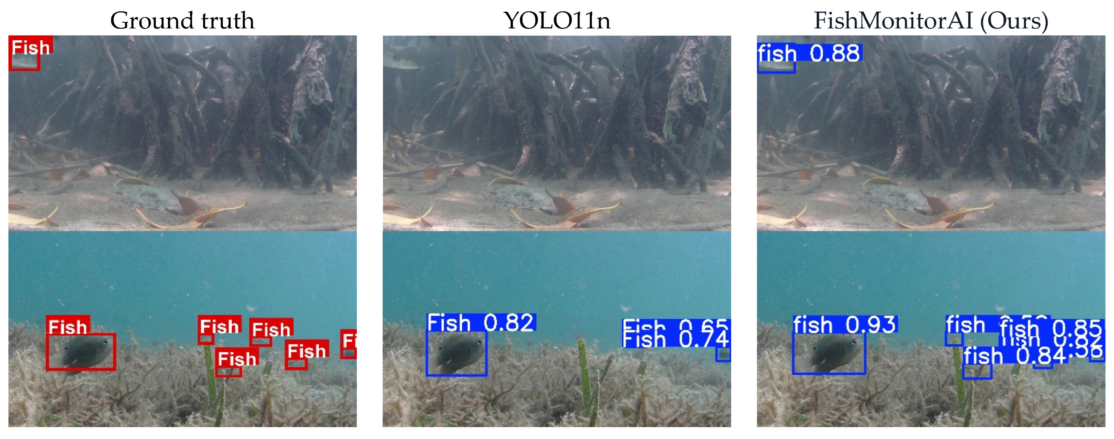
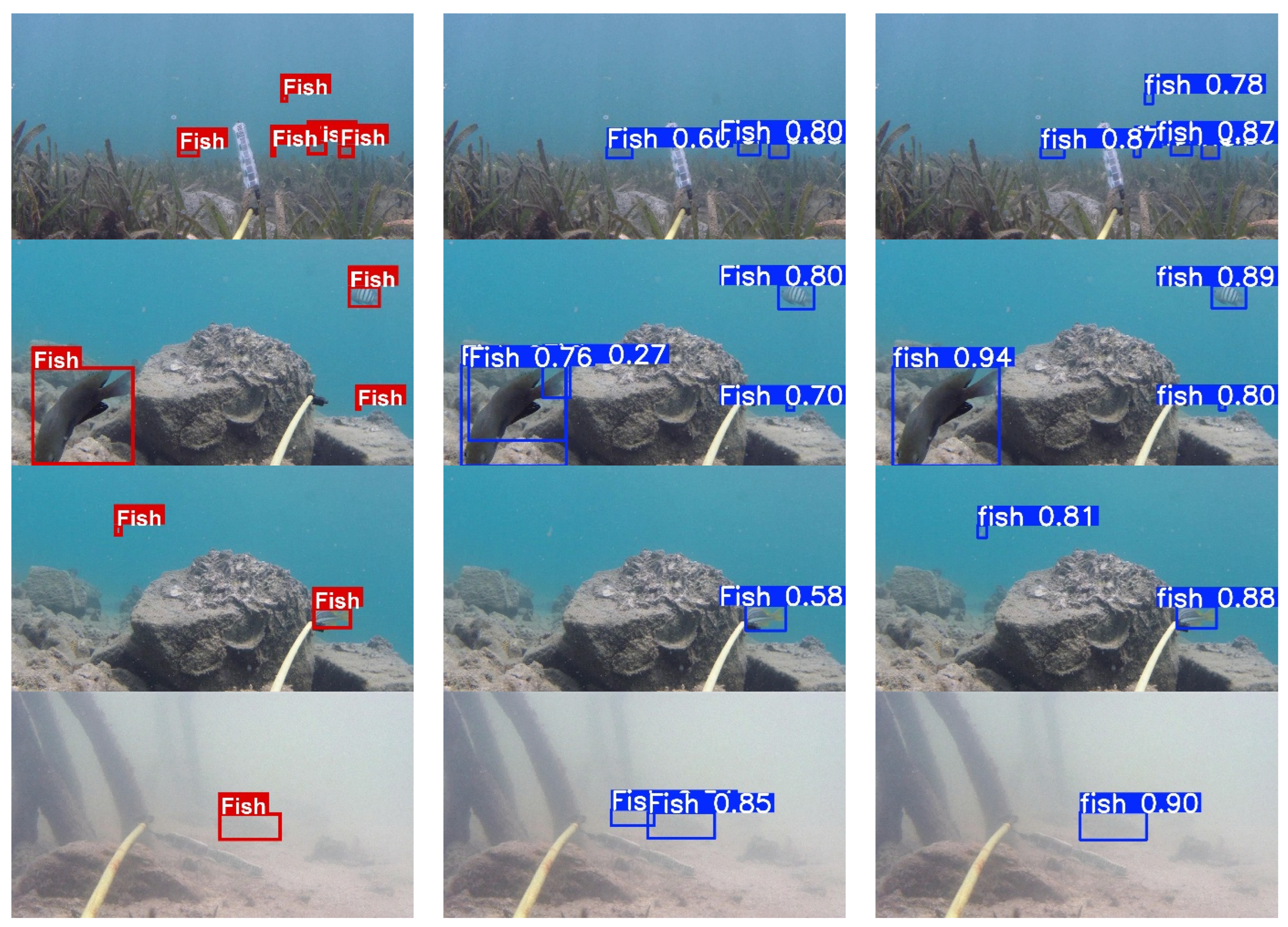
Figure 6 presents a qualitative comparison between the baseline YOLO11n model and the proposed FishMonitorAI model across several representative underwater scenes, with ground-truth annotations provided for reference. These scenes span a range of visual conditions, including cluttered backgrounds formed by dense root-like structures, seagrass beds, rocky substrates, and open water columns, thereby providing a reasonable basis for assessing detection robustness under realistic underwater imaging conditions.
Figure 6.
Qualitative comparison between YOLO11n and FishMonitorAI. Red boxes denote ground-truth annotations, while blue boxes denote model predictions.
Across scenes containing prominent, well-contrasted targets, both YOLO11n and FishMonitorAI perform comparably well, generating bounding boxes that closely align with the ground-truth annotations in terms of both localization and target coverage. This suggests that for relatively salient objects, the architectural improvements introduced in FishMonitorAI do not come at the cost of degraded performance, and the model retains detection accuracy on par with the baseline.
More notable differences between the two models emerge in scenes containing small-scale, low-contrast, or partially occluded targets. In such cases, YOLO11n tends to miss these objects entirely, failing to generate corresponding bounding boxes despite their presence in the ground truth. In contrast, FishMonitorAI exhibits clearly improved sensitivity under these conditions, successfully detecting targets that the baseline model overlooks. This behavior indicates that the enhancements incorporated into FishMonitorAI are particularly effective at strengthening feature representation for small and visually ambiguous objects, which are known to be among the most challenging cases in underwater object detection.
Furthermore, in scenes where no salient targets are present and the background is visually complex, both models correctly refrain from generating false positive detections, suggesting that the improvements introduced do not increase the model’s susceptibility to background-induced false alarms.
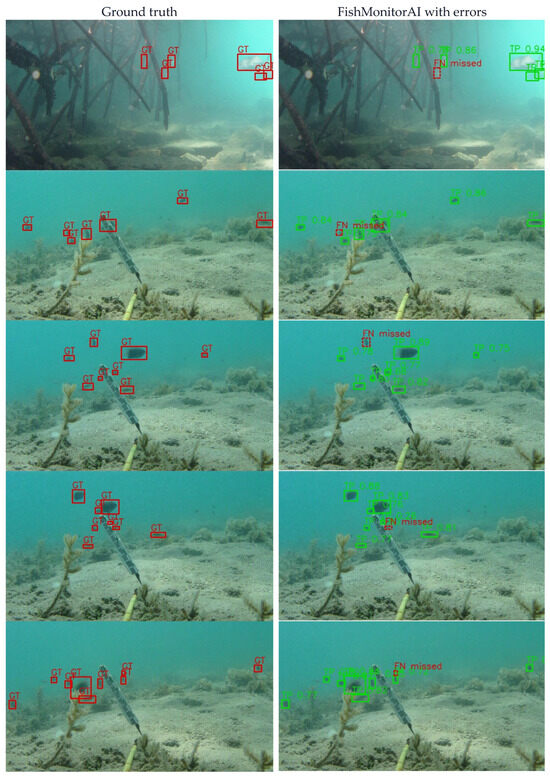
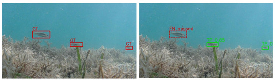
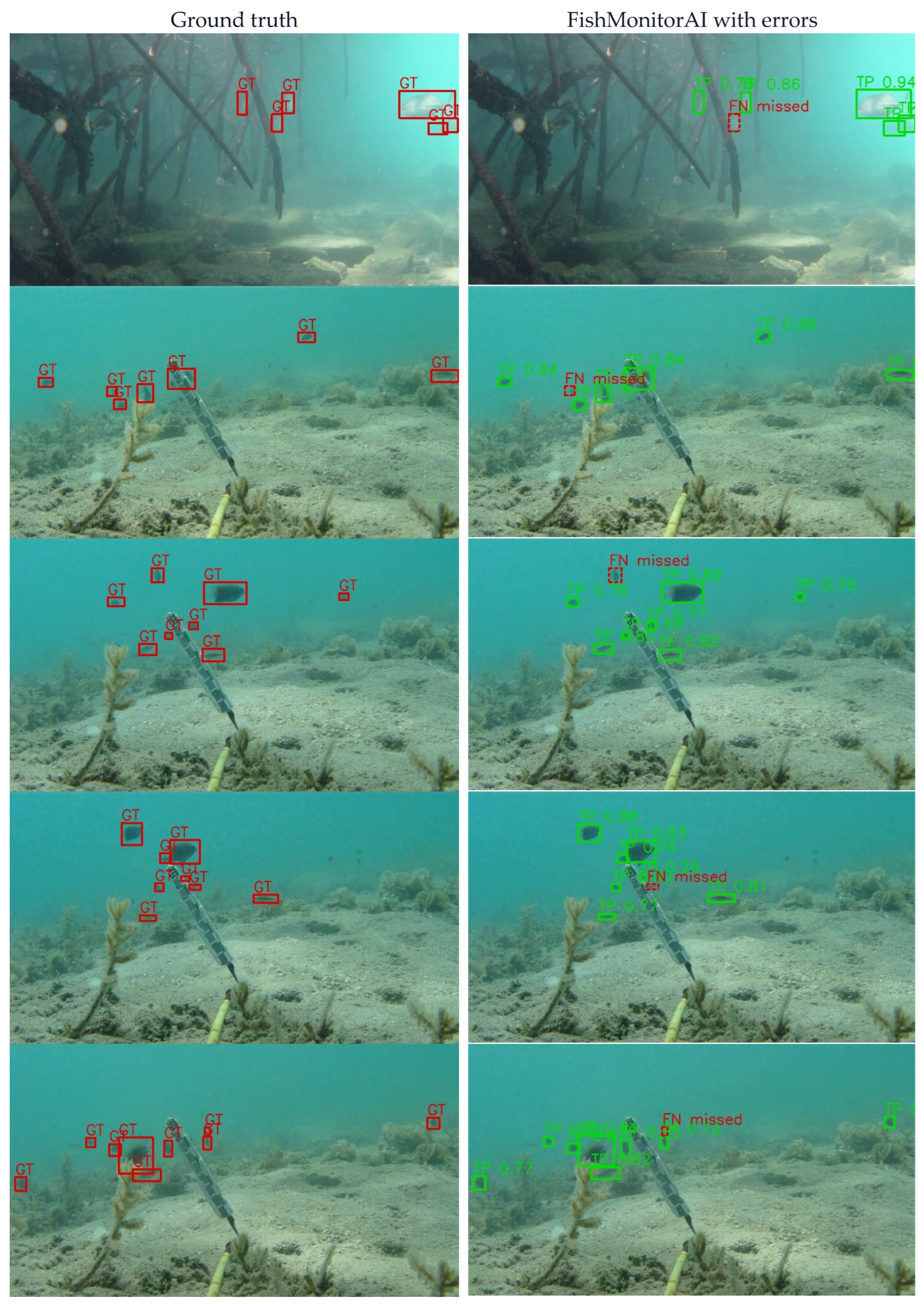
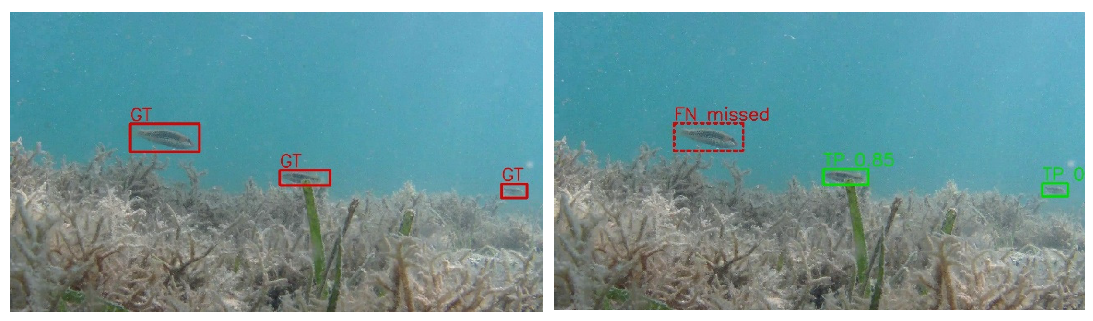
Figure 7 presents representative failure cases of FishMonitorAI across several underwater scenes with particularly challenging visual conditions. The left column shows the ground-truth (GT) annotations, while the right column presents the detection results, where true positives (TP) are shown in green and false negatives (FN) are marked as “FN missed” in red. As shown in the ground-truth annotations, these scenes contain multiple small-scale fish instances co-occurring with elongated foreign objects (e.g., survey equipment) and dense benthic vegetation, resulting in frequent partial occlusion and low target-to-background contrast. Although FishMonitorAI correctly localizes the majority of visible targets across these scenes, a small number of FN cases consistently occur, as indicated by the red “FN missed” annotations. These missed instances are predominantly associated with fish exhibiting extremely small spatial extent, weak boundary contrast, or partial occlusion by surrounding structures, whereas comparatively larger or higher-contrast targets are reliably detected as TPs. This consistent pattern suggests that the residual limitations of FishMonitorAI are primarily driven by object scale and local feature ambiguity rather than scene-level complexity alone. Future work may therefore explore high-resolution detection branches, temporal feature aggregation across video frames, or underwater image enhancement techniques (e.g., dehazing or contrast restoration) to further improve the recognition of visually degraded and extremely small fish targets.
Figure 7.
Representative failure cases of FishMonitorAI under extreme underwater conditions. Left: red boxes denote ground-truth (GT) annotations. Right: green boxes denote true-positive (TP) detections with confidence scores; red boxes labeled “FN missed” denote false-negative (FN) detections missed by the model.
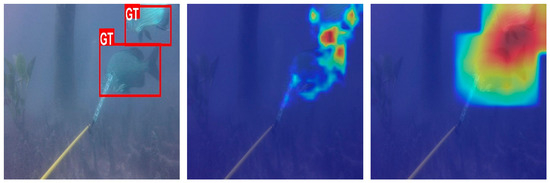
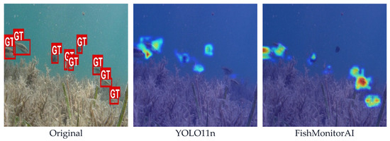
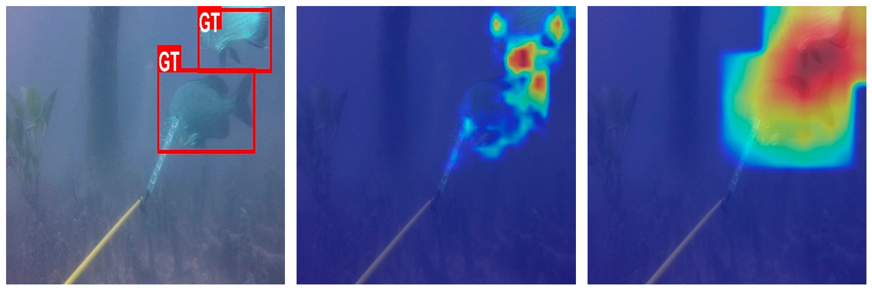
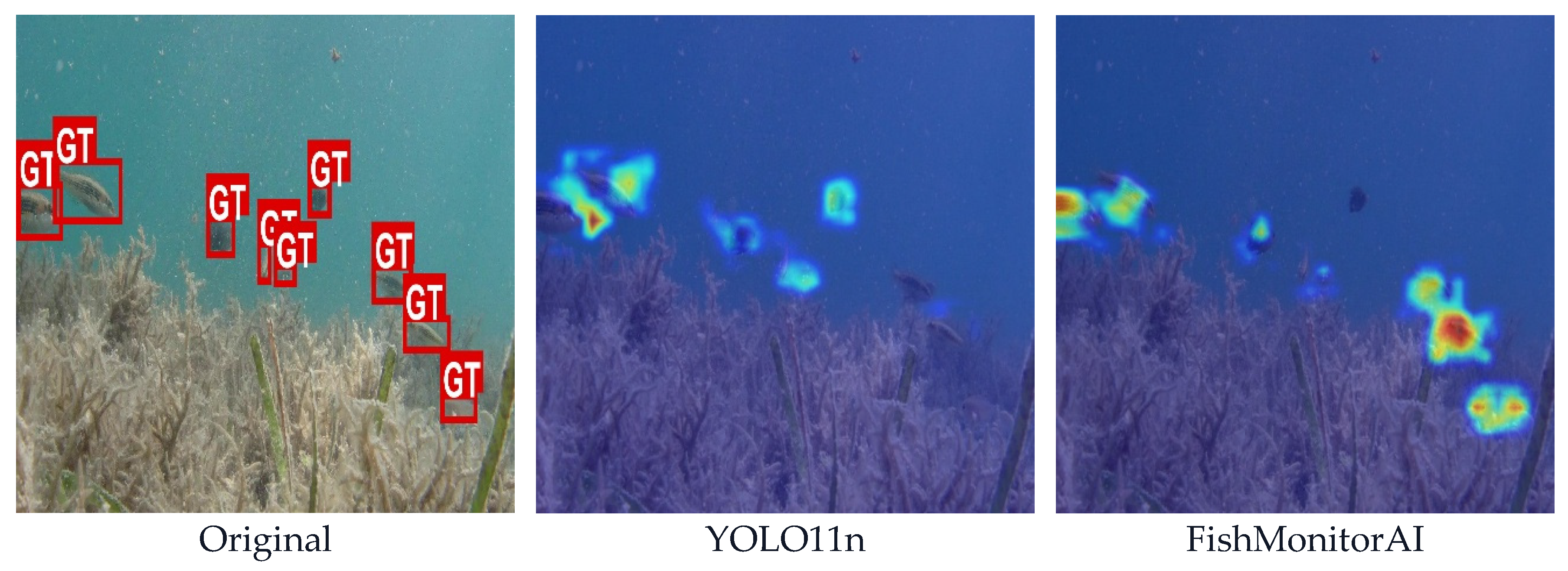
To elucidate the underlying mechanism behind the observed accuracy improvement, we employed the Grad-CAM technique to visualize the model’s regions of attention. As illustrated in Figure 8, the baseline YOLO11n model frequently produces activation regions that are dispersed across the background (background noise) or narrowly localized to only a small portion of the fish body. This limitation is particularly evident in scenes containing multiple small fish sparsely distributed, where the model exhibits only weak and scattered responses at the object locations.
Figure 8.
Heatmap visualization of model attention: YOLO11n (center) vs. FishMonitorAI (right).
In contrast, FishMonitorAI, which incorporates C3k2-DS, C2f-DS, and DySample, generates more concentrated, sharper, and more uniformly distributed activation regions across the entire object body, even under challenging environmental conditions such as high turbidity and low underwater illumination. This is clearly reflected in the deep red/orange activations that closely conform to the target object regions in both experimental scenarios. The adaptive spatial detail recovery capability of DySample enables the model to learn more discriminative features, thereby focusing accurately on salient object regions and substantially reducing false positives.
These Grad-CAM analysis results provide additional visual evidence that explains why FishMonitorAI achieves a higher mAP@0.5 while maintaining a more compact architecture compared with the baseline model.
4.5. Ablation Study
To systematically evaluate the independent and cumulative contributions of each proposed module, we conducted an ablation study by progressively integrating individual components into the baseline YOLO11n model. All experiments were performed under identical training configurations on the DEEPFISH dataset to ensure a fair comparison. The detailed results are presented in Table 3.
Table 3.
Ablation study on the contribution of each proposed component to detection performance and model efficiency.
The results indicate that C3k2-DS and C2f-DS primarily contribute to computational efficiency optimization. Specifically, C3k2-DS reduces the parameter count from 2.582 M to 2.538M (a 1.7% reduction) and GFLOPs from 6.3 to 6.2, whereas C2f-DS exhibits stronger compression capability, reducing the parameter count to 2.387 M (a 7.5% reduction) and GFLOPs to 6.0. When the two modules are combined, the model achieves the lowest GFLOPs among intermediate configurations (5.9 GFLOPs, 2.468 M parameters), demonstrating an effective synergistic effect in computational optimization. However, both modules incur a slight degradation in mAP@0.5 when operating independently, as the simplification of the backbone structure is not yet compensated for by the spatial recovery mechanism provided by the upsampling module.
In contrast, DySample yields the most substantial improvement in detection accuracy among the individual modules, raising mAP@0.5 from 97.1% to 97.8%, with Precision and Recall reaching 96.8% and 95.8%, respectively. This demonstrates that the adaptive upsampling mechanism of DySample enables the model to recover fine-grained spatial features more effectively than conventional interpolation methods. When DySample is integrated with either C3k2-DS or C2f-DS, mAP@0.5 further increases to 98.0% and 97.9%, respectively, while preserving the downward trend in parameter count, thereby confirming the complementary nature of these modules.
When all three modules are integrated simultaneously, FishMonitorAI achieves an optimal balance, attaining the highest mAP@0.5 of 98.2% (an improvement of 1.1 percentage points over the baseline), while simultaneously reducing the parameter count to 2.462M (a 4.6% reduction) and GFLOPs to 5.9 (a 6.3% reduction). These findings confirm that C3k2-DS and C2f-DS primarily improve computational efficiency in the backbone and neck, respectively, while DySample enhances detection sensitivity through adaptive upsampling in the neck. Together, these results indicate that C3k2-DS and C2f-DS primarily improve computational efficiency, while DySample contributes more directly to detection accuracy; their combination provides the most favorable overall balance among the evaluated configurations.
5. Discussion
FishMonitorAI achieves an mAP@0.5 of 98.2% on DeepFish and outperforms the YOLO11n baseline (97.1%) under the same experimental conditions. For broader contextual comparison, previously published methods such as YOLO-Fish (76.56%/75.70%) [50], AquaYOLO (90.9%) [52], Mobile-YOLO (+1.6% over baseline) [53], and YOLO-PWSL (96.1%) [54] are also considered; however, these reported results are not directly comparable because they were obtained using different datasets, classes, conditions, and baseline detectors. The gap over YOLO-PWSL likely reflects such differences rather than a proportionally larger contribution from the proposed modules: YOLO-PWSL is tested on field data with turbidity, occlusion, and shape distortion, while DeepFish is a curated single-class benchmark evaluated on a stronger baseline (YOLO11n vs. YOLOv5s). Although Mobile-YOLO [53] and FishMonitorAI both employ DySample and lightweight convolutional design, they follow different architectural strategies. Mobile-YOLO is derived from YOLOv8 and introduces a Mobile-Nano backbone, the LDtect lightweight detection head, DySample, and HWD-based downsampling. In contrast, FishMonitorAI is built upon YOLO11n and modifies its native C3k2-based structure by introducing C3k2-DS in the backbone, replacing the C3k2 feature-fusion blocks in the neck with C2f-DS, and integrating DySample while retaining the original Detect head. Therefore, the contribution of FishMonitorAI should be understood as a distinct YOLO11n-based lightweight architectural design rather than as the introduction of DySample or depthwise separable convolution themselves. The direct latency measurements further indicate that the reduced theoretical complexity of FishMonitorAI translates into lower inference latency on the evaluated GTX 1650 Ti platform. FishMonitorAI achieves 40.078 ms/image compared with 43.685 ms/image for YOLO11n under identical benchmark conditions. This observation is particularly relevant because reductions in GFLOPs, especially in architectures employing depthwise separable convolutions, do not necessarily guarantee lower wall-clock latency. Nevertheless, inference performance remains hardware- and runtime-dependent, and dedicated evaluation on representative embedded platforms is still required. Likewise, the closely matched training and validation loss curves in Figure 5 indicate stable convergence, but they do not by themselves exclude the possibility of overfitting. This is particularly relevant because the DeepFish images originate from only 20 habitats and the dataset was divided using a random train/validation/test split rather than a habitat-disjoint protocol. Consequently, visually similar images from the same habitat may occur in both the training and test subsets. The near-99% mAP@0.5 observed during validation may therefore partly reflect the relatively constrained single-class detection setting and shared habitat characteristics across the data splits rather than generalization to completely unseen underwater environments. Accordingly, the reported results should be interpreted as performance under the current DeepFish split rather than as evidence of habitat-independent generalization. A further limitation is that each model configuration was evaluated based on a single training run. Therefore, run-to-run variability was not quantified, and the small difference in mAP@0.5 between FishMonitorAI (98.2%) and YOLOv8n (98.1%) should not be interpreted as statistically significant superiority. The present results should instead be regarded as indicative of competitive performance under the adopted experimental protocol. In addition, although FishMonitorAI achieves the highest mAP@0.5, its mAP@0.5:0.95 of 76.9% is lower than that of YOLOv8n (77.6%) and YOLOv10n (77.0%). This suggests that the performance gain observed at IoU = 0.5 does not fully extend to stricter localization thresholds. One possible explanation is that the proposed architecture improves sensitivity to small, low-contrast, and partially occluded fish, while minor bounding-box localization errors are penalized more strongly at higher IoU thresholds, particularly for small objects. An additional limitation concerns the scope of the detection task. The present experiments evaluate FishMonitorAI only as a single-class detector in which all targets are labeled as “fish”. Consequently, the study does not directly assess species identification, disease diagnosis, individual tracking, biomass estimation, behavioral analysis, or selective fishing. These functions should therefore be regarded as potential downstream applications rather than demonstrated capabilities of the current model. Future work may extend FishMonitorAI with task-specific classification, tracking, or health-monitoring modules to evaluate these applications explicitly. We regard these issues as important limitations of the present study. Future work will therefore include repeated training with multiple random seeds and statistical analysis of run-to-run variability, together with habitat-wise data partitioning, leave-one-habitat-out evaluation, and cross-dataset validation on independent benchmarks such as OzFish and DePondFi to more rigorously assess the robustness and generalization capability of FishMonitorAI under unseen environmental conditions.
6. Conclusions
This paper presents a novel approach to fish detection in aquatic environments through the development of the FishMonitorAI model. Motivated by the limitations of existing methods in handling small objects under complex underwater conditions, FishMonitorAI introduces three targeted architectural modifications to YOLO11n: C3k2-DS blocks in the backbone, C2f-DS feature-fusion blocks in the neck, and DySample-based dynamic upsampling in the neck, while retaining the original Detect head.
Through experimental evaluation on DeepFish, FishMonitorAI demonstrates a favorable balance between detection accuracy, model complexity, and inference efficiency. The proposed model achieves an mAP@0.5 of 98.2% while requiring 5.9 GFLOPs and 2.462 M parameters. Direct inference measurements on the NVIDIA GTX 1650 Ti further show a latency of 40.078 ms/image, compared with 43.685 ms/image for the YOLO11n baseline under the same benchmark conditions. These results indicate that the proposed architectural modifications reduce theoretical computational complexity while also achieving lower measured inference latency on the evaluated GPU platform. The ablation study and Grad-CAM analyses further illustrate the respective and complementary contributions of the proposed modules. However, the present evaluation is based on a random train/validation/test split of DeepFish rather than a habitat-disjoint protocol. Therefore, the reported results should not be interpreted as evidence of generalization to completely unseen underwater environments. The present work evaluates only single-class fish detection; therefore, higher-level tasks such as species recognition, health assessment, tracking, biomass estimation, and selective harvesting remain future research directions. Future work will focus on habitat-wise and leave-one-habitat-out evaluation, as well as cross-dataset validation on independent underwater fish datasets, to more rigorously assess model robustness and generalization. The lightweight architecture of FishMonitorAI indicates potential suitability for deployment on resource-constrained platforms; however, the present latency measurements were obtained only on the evaluated GPU platform. Future work will therefore focus on embedded-device validation, including latency, memory-footprint, and, where feasible, power-consumption measurements, together with model compression techniques such as knowledge distillation and quantization.
Author Contributions
Conceptualization, methodology, formal analysis, investigation, resources, writing, visualization—V.L., M.A., M.U., A.S., A.F., A.V., and A.R. All authors have read and agreed to the published version of the manuscript.
Funding
This research was funded by the Russian Science Foundation, grant number 26-19-00326, https://rscf.ru/en/project/26-19-00326/ (accessed on 4 September 2026).
Institutional Review Board Statement
As this manuscript does not involve any research on animals or human subjects, ethical approval from an Institutional Review Board was not required.
Informed Consent Statement
Not applicable.
Data Availability Statement
The original contributions presented in this study are included in the article. Further inquiries can be directed to the corresponding author.
Conflicts of Interest
The authors declare no conflicts of interest.
Abbreviations
The following abbreviations are used in this manuscript:
| A2 | Area Attention |
| C2f-DS | C2f (CSP Bottleneck with 2 convolutions) with Depthwise Separable Convolutions |
| C2PSA | Cross Stage Partial with Spatial Attention |
| C3k2-DS | CSP Block with 3 convolutions and 2 kernel/bottleneck sizes, utilizing Depthwise Separable Convolutions |
| CARAFE | Content-Aware ReAssembly of FEatures |
| CFC | Caltech Fish Counting |
| CmBN | Cross mini-Batch Normalization |
| CSP | Cross Stage Partial |
| DETR | DEtection TRansformer |
| DSConv | Depthwise Separable Convolution |
| DySample | Dynamic Upsampling |
| FLOPs | Floating Point Operations |
| FN | False Negative |
| FP | False Positive |
| FPN | Feature Pyramid Network |
| FPS | Frames Per Second |
| GT | Ground Truth |
| GELAN | Generalized Efficient Layer Aggregation Network |
| GFLOPs | Giga Floating-Point Operations |
| Grad-CAM | Gradient-weighted Class Activation Mapping |
| HSV | Hue, Saturation, Value |
| HWD | Haar Wavelet Downsampling |
| IoU | Intersection over Union |
| LDtect | Lightweight Detection head |
| LTS | Long-Term Support |
| mAP | mean Average Precision |
| MLP | Multi-Layer Perceptron |
| NMS | Non-Maximum Suppression |
| PANet | Path Aggregation Network |
| PGI | Programmable Gradient Information |
| R-CNN | Region-based Convolutional Neural Network |
| R-ELAN | Residual Efficient Layer Aggregation Network |
| ResNet | Residual Network |
| RT-DETR | Real-Time DEtection TRansformer |
| SGD | Stochastic Gradient Descent |
| SPP | Spatial Pyramid Pooling |
| SPPF | Spatial Pyramid Pooling Fast |
| SSD | Single-Shot MultiBox Detector |
| TP | True Positive |
| VGG | Visual Geometry Group |
| YOLO | You Only Look Once |
References
- Wu, Y.; Duan, Y.; Wei, Y.; An, D.; Liu, J. Application of intelligent and unmanned equipment in aquaculture: A review. Comput. Electron. Agric. 2022, 199, 107201. [Google Scholar] [CrossRef] [Scilit]
- Tanaka, K.; Tomiyasu, M.; Kusaka, R.; Sugiyama, S.; Podolskiy, E.A.; Fujimori, Y. Artisanal longline fishing for Greenland halibut (Reinhardtius hippoglossoides) operated under sea ice using a metal plate kite in northwest Greenland. Fish. Res. 2025, 281, 107203. [Google Scholar] [CrossRef] [Scilit]
- Guzmán, M.A.E.; Barretto, J.W.; López, M.D.R.P.; Cruz, C.C. Sustainability of fishing cooperatives in the Gulf of Mexico: A case study. Fish. Res. 2024, 279, 107105. [Google Scholar] [CrossRef] [Scilit]
- Chen, J.-H.; Sung, W.-T.; Lin, G.-Y. Automated monitoring system for the fish farm aquaculture environment. In Proceedings of the IEEE International Conference on Systems, Man, and Cybernetics (SMC 2015), Kowloon Tong, Hong Kong, China, 9–12 October 2015; pp. 1161–1166. [Google Scholar]
- Amuthakkannan, R.; Vijayalakshmi, K.; Al Araimi, S.; Al Tobi, M.A. A review to do fishermen boat automation with artificial intelligence for sustainable fishing experience ensuring safety, security, navigation and sharing information for Omani fishermen. J. Mar. Sci. Eng. 2023, 11, 630. [Google Scholar] [CrossRef] [Scilit]
- Qiao, M.; Wang, D.; Tuck, G.N.; Little, L.R.; Punt, A.E.; Gerner, M. Deep learning methods applied to electronic monitoring data: Automated catch event detection for longline fishing. ICES J. Mar. Sci. 2021, 78, 25–35. [Google Scholar] [CrossRef] [Scilit]
- Karningsih, P.D.; Kusumawardani, R.; Syahroni, N.; Mulyadi, Y.; Saad, M.S.B.M. Automated fish feeding system for an offshore aquaculture unit. IOP Conf. Ser. Mater. Sci. Eng. 2021, 1072, 012073. [Google Scholar] [CrossRef] [Scilit]
- Xu, H.; Moreira, L.; Guedes Soares, C. Maritime autonomous vessels. J. Mar. Sci. Eng. 2023, 11, 168. [Google Scholar] [CrossRef] [Scilit]
- Piecho-Santos, A.M.P.; Hinostroza, M.A.; Rosa, T.; Soares, C.G. Autonomous observing systems in fishing vessels. Marit. Technol. Eng. 2021, 52, 805–808. [Google Scholar] [CrossRef] [Scilit]
- Zhao, L.; Wang, F.; Bai, Y. Route planning for autonomous vessels based on improved artificial fish swarm algorithm. Ships Offshore Struct. 2023, 18, 897–906. [Google Scholar] [CrossRef] [Scilit]
- Bogue, R. Underwater robots: A review of technologies and applications. Ind. Robot Int. J. 2015, 42, 186–191. [Google Scholar] [CrossRef] [Scilit]
- Yuh, J. Design and control of autonomous underwater robots: A survey. Auton. Robot. 2000, 8, 7–24. [Google Scholar] [CrossRef] [Scilit]
- Hsieh, C.L.; Chang, H.Y.; Chen, F.H.; Liou, J.H.; Chang, S.K.; Lin, T.T. A simple and effective digital imaging approach for tuna fish length measurement compatible with fishing operations. Comput. Electron. Agric. 2011, 75, 44–51. [Google Scholar] [CrossRef] [Scilit]
- Don Chua, W.F.; Lim, C.L.; Koh, Y.Y.; Kok, C.L. A novel IoT photovoltaic-powered water irrigation control and monitoring system for sustainable city farming. Electronics 2024, 13, 676. [Google Scholar] [CrossRef] [Scilit]
- Saqib, M.; Khokher, M.R.; Yuan, X.; Untiedt, C.; Devine, C. Fishing event detection and species classification using computer vision and artificial intelligence for electronic monitoring. Fish. Res. 2024, 280, 107141. [Google Scholar] [CrossRef] [Scilit]
- Yu, H.; Li, X.; Feng, Y.; Han, S. Multiple attentional path aggregation network for marine object detection. Appl. Intell. 2023, 53, 2434–2451. [Google Scholar] [CrossRef] [Scilit]
- Krizhevsky, A.; Sutskever, I.; Hinton, G.E. ImageNet classification with deep convolutional neural networks. In Proceedings of the 26th Annual Conference on Neural Information Processing Systems (NIPS 2012), Lake Tahoe, NV, USA, 3–6 December 2012; pp. 84–90. [Google Scholar]
- Girshick, R.; Donahue, J.; Darrell, T.; Malik, J. Rich feature hierarchies for accurate object detection and semantic segmentation. In Proceedings of the IEEE Conference on Computer Vision and Pattern Recognition (CVPR 2014), Columbus, OH, USA, 23–28 June 2014; pp. 580–587. [Google Scholar]
- Girshick, R. Fast R-CNN. In Proceedings of the IEEE International Conference on Computer Vision (ICCV 2015), Santiago, Chile, 7–13 December 2015; pp. 1440–1448. [Google Scholar]
- Ren, S.; He, K.; Girshick, R.; Sun, J. Faster R-CNN: Towards real-time object detection with region proposal networks. Adv. Neural Inf. Process. Syst. 2015, 28, 91–99. [Google Scholar] [CrossRef] [Scilit] [PubMed]
- He, K.; Gkioxari, G.; Dollár, P.; Girshick, R. Mask R-CNN. In Proceedings of the IEEE International Conference on Computer Vision (ICCV 2017), Venice, Italy, 22–29 October 2017; pp. 2961–2969. [Google Scholar]
- Redmon, J.; Divvala, S.; Girshick, R.; Farhadi, A. You only look once: Unified, real-time object detection. In Proceedings of the IEEE Conference on Computer Vision and Pattern Recognition (CVPR 2016), Las Vegas, NV, USA, 27–30 June 2016; pp. 779–788. [Google Scholar]
- Redmon, J.; Farhadi, A. YOLO9000: Better, faster, stronger. In Proceedings of the IEEE Conference on Computer Vision and Pattern Recognition (CVPR 2017), Honolulu, HI, USA, 21–26 July 2017; pp. 6517–6525. [Google Scholar]
- Redmon, J.; Farhadi, A. YOLOv3: An incremental improvement. arXiv 2018, arXiv:1804.02767. [Google Scholar]
- Bochkovskiy, A.; Wang, C.Y.; Liao, H. YOLOv4: Optimal speed and accuracy of object detection. arXiv 2020, arXiv:2004.10934. [Google Scholar]
- Jocher, G.; Chaurasia, A.; Qiu, J. Ultralytics YOLOv8. Available online: https://docs.ultralytics.com/models/yolov8 (accessed on 12 May 2026).
- Wang, A.; Chen, H.; Liu, L.; Chen, K.; Lin, Z.; Han, J.; Ding, G. YOLOv10: Real-time end-to-end object detection. arXiv 2024, arXiv:2405.14458. [Google Scholar]
- Jocher, G.; Qiu, J. Ultralytics YOLO11. Available online: https://docs.ultralytics.com/models/yolo11 (accessed on 12 May 2026).
- Tian, Y. YOLOv12: Attention-centric real-time object detectors. arXiv 2025, arXiv:2502.12524. [Google Scholar]
- Liu, W.; Anguelov, D.; Erhan, D.; Szegedy, C.; Reed, S.; Fu, C.Y.; Berg, A.C. SSD: Single shot multibox detector. In Proceedings of the European Conference on Computer Vision (ECCV 2016), Amsterdam, The Netherlands, 11–14 October 2016; pp. 21–37. [Google Scholar]
- Lin, T.Y.; Goyal, P.; Girshick, R.; He, K.; Dollár, P. Focal loss for dense object detection. In Proceedings of the IEEE International Conference on Computer Vision (ICCV 2017), Venice, Italy, 22–29 October 2017; pp. 2980–2988. [Google Scholar]
- Carion, N.; Massa, F.; Synnaeve, G.; Usunier, N.; Kirillov, A.; Zagoruyko, S. End-to-end object detection with transformers. In Proceedings of the European Conference on Computer Vision (ECCV 2020), Glasgow, UK, 23–28 August 2020; pp. 213–229. [Google Scholar]
- Vaswani, A.; Shazeer, N.; Parmar, N.; Uszkoreit, J.; Jones, L.; Gomez, A.N.; Kaiser, Ł.; Polosukhin, I. Attention is all you need. Adv. Neural Inf. Process. Syst. 2017, 30, 5998–6008. [Google Scholar] [CrossRef] [Scilit]
- Liu, W.; Lu, H.; Fu, H.; Cao, Z. Learning to upsample by learning to sample. In Proceedings of the IEEE/CVF International Conference on Computer Vision (ICCV 2023), Paris, France, 1–6 October 2023; pp. 6004–6014. [Google Scholar]
- Howard, A.G.; Zhu, M.; Chen, B.; Kalenichenko, D.; Wang, W.; Weyand, T.; Andreetto, M.; Adam, H. MobileNets: Efficient convolutional neural networks for mobile vision applications. arXiv 2017, arXiv:1704.04861. [Google Scholar]
- Sandler, M.; Howard, A.; Zhu, M.; Zhmoginov, A.; Chen, L.C. MobileNetV2: Inverted residuals and linear bottlenecks. In Proceedings of the IEEE Conference on Computer Vision and Pattern Recognition (CVPR 2018), Salt Lake City, UT, USA, 18–23 June 2018; pp. 4510–4520. [Google Scholar]
- Saleh, A.; Laradji, I.H.; Konovalov, D.A.; Bradley, M.; Vazquez, D.; Sheaves, M. A realistic fish-habitat dataset to evaluate algorithms for underwater visual analysis. Sci. Rep. 2020, 10, 14671. [Google Scholar] [CrossRef] [Scilit] [PubMed]
- Simonyan, K.; Zisserman, A. Very deep convolutional networks for large-scale image recognition. arXiv 2014, arXiv:1409.1556. [Google Scholar]
- Lin, T.Y.; Dollár, P.; Girshick, R.; He, K.; Hariharan, B.; Belongie, S. Feature pyramid networks for object detection. In Proceedings of the IEEE Conference on Computer Vision and Pattern Recognition (CVPR 2017), Honolulu, HI, USA, 21–26 July 2017; pp. 2961–2969. [Google Scholar]
- He, K.; Zhang, X.; Ren, S.; Sun, J. Deep residual learning for image recognition. In Proceedings of the IEEE Conference on Computer Vision and Pattern Recognition (CVPR 2016), Las Vegas, NV, USA, 27–30 June 2016; pp. 770–778. [Google Scholar]
- Liu, S.; Qi, L.; Qin, H.; Shi, J.; Jia, J. Path aggregation network for instance segmentation. In Proceedings of the IEEE Conference on Computer Vision and Pattern Recognition (CVPR 2018), Salt Lake City, UT, USA, 18–23 June 2018; pp. 7700–7709. [Google Scholar]
- Jocher, G. Yolov5. Available online: https://docs.ultralytics.com/models/yolov5 (accessed on 12 May 2026).
- Wang, C.Y.; Yeh, I.H.; Mark Liao, H.Y. YOLOv9: Learning what you want to learn using programmable gradient information. In Proceedings of the European Conference on Computer Vision (ECCV 2024), Milan, Italy, 29 September–4 October 2024; pp. 1–21. [Google Scholar]
- Sapkota, R.; Karkee, M. YOLO11 and vision transformers based 3D pose estimation of immature green fruits in commercial apple orchards for robotic thinning. arXiv 2024, arXiv:2410.19846. [Google Scholar]
- Karimanzira, D. Comprehensive Fish Feeding Management in Pond Aquaculture Based on Fish Feeding Behavior Analysis Using a Vision Language Model. Aquac. J. 2025, 5, 15. [Google Scholar] [CrossRef] [Scilit]
- Soifer, V.; Fursov, V.; Kharitonov, S. Kalman Filter for a Particular Class of Dynamic Object Images. Inform. Autom. 2024, 23, 953–968. [Google Scholar] [CrossRef] [Scilit]
- Tamut, H.; Ghosh, R.; Gosh, K.; Siddique, M.A.S. Enhancing Disease Detection in the Aquaculture Sector Using Convolutional Neural Networks Analysis. Aquac. J. 2025, 5, 6. [Google Scholar] [CrossRef] [Scilit]
- Sirota, A.; Akimov, A.; Otyrba, R. Image Warping and Its Application for Data Augmentation when Training Deep Neural Networks. Inform. Autom. 2024, 23, 407–435. [Google Scholar] [CrossRef] [Scilit]
- Barbosa, L.A.; Maciel, M.S.; Gomes, F.R.; Jawad, L.; Queiroz, C.; Viana, D.C. Evaluating morphometric variations in Tocantins River fish: Implications for conservation. Acta Sci. Anim. Sci. 2025, 47, e72269. [Google Scholar] [CrossRef] [Scilit]
- Al Muksit, A.; Hasan, F.; Emon, M.F.H.B.; Haque, M.R.; Anwary, A.R.; Shatabda, S. YOLO-Fish: A robust fish detection model to detect fish in realistic underwater environment. Ecol. Inform. 2022, 72, 101847. [Google Scholar] [CrossRef] [Scilit]
- Ouis, M.Y.; Akhloufi, M. YOLO-based fish detection in underwater environments. Environ. Sci. Proc. 2023, 29, 44. [Google Scholar] [CrossRef] [Scilit]
- Vijayalakshmi, M.; Sasithradevi, A. AquaYOLO: Advanced YOLO-based fish detection for optimized aquaculture pond monitoring. Sci. Rep. 2025, 15, 6151. [Google Scholar] [CrossRef] [Scilit] [PubMed]
- Jiang, H.; Zhao, J.; Ma, F.; Yang, Y.; Yi, R. Mobile-YOLO: A lightweight object detection algorithm for four categories of aquatic organisms. Fishes 2025, 10, 348. [Google Scholar] [CrossRef] [Scilit]
- Lei, L.; Tang, Y.; Zhang, W.; Tang, Q.; Hao, H. YOLO-PWSL-Enhanced Robotic Fish: An integrated object detection system for underwater monitoring. Appl. Sci. 2025, 15, 7052. [Google Scholar] [CrossRef] [Scilit]
- Van Nghia, L.; Van Tuyen, T.; Figurek, A.; Ronzhin, A. Fish disease detection using enhanced YOLOv11 for application in aquatic robots. In Proceedings of the 10th International Conference on Interactive Collaborative Robotics (ICR 2025), Hanoi, Vietnam, 10–13 November 2025; pp. 202–218. [Google Scholar]
- Milovanović, V.; Figurek, A.; Ogij, O.; Le, V.; Ronzhin, A.; Markou, M. AIoT-Based Aquaponics: A Responsible Decision-Support Framework for Smart Water Management and Sustainable Aquaculture. Environments 2026, 13, 427. [Google Scholar] [CrossRef] [Scilit]
- Ma, N.; Zhang, X.; Zheng, H.T.; Sun, J. ShuffleNet V2: Practical guidelines for efficient CNN architecture design. In Proceedings of the European Conference on Computer Vision (ECCV 2018), Munich, Germany, 8–14 September 2018; pp. 116–131. [Google Scholar]
- Wang, J.; Chen, K.; Xu, R.; Liu, Z.; Loy, C.C.; Lin, D. CARAFE: Content-aware reassembly of features. In Proceedings of the IEEE/CVF International Conference on Computer Vision (ICCV 2019), Seoul, South Korea, 27 October–2 November 2019; pp. 3007–3016. [Google Scholar]

Disclaimer/Publisher’s Note: The statements, opinions and data contained in all publications are solely those of the individual author(s) and contributor(s) and not of MDPI and/or the editor(s). MDPI and/or the editor(s) disclaim responsibility for any injury to people or property resulting from any ideas, methods, instructions or products referred to in the content. |
© 2026 by the authors. Licensee MDPI, Basel, Switzerland. This article is an open access article distributed under the terms and conditions of the Creative Commons Attribution (CC BY) license.