


Abstract
The Causal Quantum Spacetime Theory (CQST) treats spacetime as emergent from a discrete causal substrate, the quantum spacetime regenerating (QSR) lattice, assembling its geometric, holographic, quantum-foundational and phenomenological strands. The framework identifies the QSR lattice with Fuller’s Isotropic Vector Matrix and adopts holographic scaling together with the Bekenstein–Hawking one-quarter factor. The vacuum causal density, the squared ratio of the Planck length to the de Sitter radius fixed by Λ, is a constant of spacetime; its logarithmic relation to the fine-structure constant α is a one-parameter calibration predicting no drift. The reduced Planck constant is reinterpreted as the action of one causal tick. The empirical content lies in the photon sector: the discrete electromagnetic action on the face-centred cubic lattice is built over its twelve nearest-neighbour vectors and the propagator obtained within the Brillouin zone. The linear coefficient vanishes identically and helicity-odd birefringence is excluded by inversion. In the twelve-fold FCC formulation, the leading quadratic correction is subluminal in every direction, with isotropic part 1/20 in units of the squared nearest-neighbour separation and an octahedral modulation of 5/18. The quadratic sector lies far below current sensitivity; the first two predictions are exact falsification tests of the assumed lattice symmetries.
1. Introduction
Reconciling general relativity with quantum mechanics remains one of the central open problems of fundamental physics. The Causal Quantum Spacetime Theory (CQST) proposes that spacetime emerges as a statistical description of a discrete causal graph G, rather than a pre-existing continuum. Its elementary degrees of freedom are quantum spacetime regenerating (QSR) nodes, interpreted as minimal regenerating units of spacetime. Rather than representing points embedded in a manifold, QSR nodes generate large-scale geometry through connectivity, causal density and dynamical transport. Directed edges Uij encode elementary causal transfer processes, while metric properties arise only after coarse-graining. In this sense CQST belongs to the wider family of approaches that derive geometry from combinatorial or causal structure, including causal-set theory, loop quantum gravity and Causal Dynamical Triangulations (CDT), while placing particular emphasis on regeneration, torsion and vacuum fixed-point dynamics [1,2,3,4,5,6].
Why does the reduced Planck constant ℏ have the value and dimensions it does? In standard formulations ℏ is measured and inserted as an empirical constant; its consequences are enormous—stable atoms, quantized spectra, uncertainty relations, wave dynamics—yet its origin is not derived. CQST proposes that ℏ is the quantitative signature of discrete causal structure at the QSR scale [2,7,8]. This should be intended (in the context of the CQST framework) as a reinterpretation rather than a derivation: the identification fixes the meaning and dimensions of ℏ, not its numerical value, which still enters through the lattice parameters.
The aim of this paper is to present the geometric and quantum-foundational strands as one consistent framework. Where a relation is a fit rather than a prediction, this is stated explicitly; where a proposed identification is not supported by the dynamics or observations, its limitations are reported directly.
The paper is organised as follows. Section 2 states the formal apparatus of the framework: the effective Lagrangian and the emergent metric, the discrete tick dynamics, the identification of the QSR lattice with the Isotropic Vector Matrix (IVM), the definitions of the causal density and of the fine-structure constant, the operational definition of the causal tick, and the deformed dispersion relation that supplies the observational test. Section 3 collects the consequences that follow from this apparatus, from the vacuum fixed point and holographic scaling to the C0–α relation, the recovery of the standard quantum relations, and the confrontation of the dispersion prediction with gamma-ray-burst data. Section 4 discusses the logical structure of the framework, its speculative sectors, its limitations and the research priorities it generates. Section 5 concludes. Appendix A presents the representation-theoretic analysis of the twelve-channel bond space and its implications for lattice uniqueness.
2. Theoretical Framework
CQST is a theoretical framework rather than an experimental study; this section therefore states the postulates, definitions and mathematical structures from which every result reported in Section 3 is obtained, together with the observational quantities used to test them. No new data are generated in this work. The empirical inputs are the measured values of the Hubble constant and of the fine-structure constant, introduced in Section 2.7, and the published gamma-ray-burst and atmospheric-Cherenkov timing limits collected in Section 3.15.
2.1. The CQST Lagrangian and Emergent Geometry
In the continuum description, the QSR order parameter is represented by a real scalar field ρ, while torsion is treated as an auxiliary Einstein–Cartan degree of freedom. No curvature term is included, and no gravitational field equations are derived in this paper; the passage from the discrete dynamics to the Einstein equations is the principal missing element of the framework and is listed in Section 4.6. The corresponding effective Lagrangian is
where denotes the characteristic mass scale of the torsional sector. In Einstein–Cartan–Sciama–Kibble (ECSK) gravity the corresponding scale is naturally expected to be of order , although no derivation is attempted within CQST. The normalisation adopted in Equation (1) makes the coupling dimensionless, and the stability condition is . The torsion field is treated throughout as an auxiliary, non-propagating degree of freedom; therefore, the quadratic term proportional to should be interpreted as an algebraic mass term rather than as a kinetic term.
The vacuum structure of the scalar sector is determined by the Landau–Ginzburg potential
and torsion is defined by
where (x,y) denotes a connected correlator of the causal transport, normalised to unity at coincidence, , and decaying on the scale ℓQSR. The disconnected quantity Tr[U(x,y)U(y,x)] cannot be used: for unitary transport one has and therefore identically, implying that its mixed second derivative vanishes. With the definition above, σ2(x,y) plays the role of the squared geodesic interval and the coincidence limit y → x reproduces the metric in the standard Synge form. The construction is stated here as a schematic ansatz: no proof is offered that the microscopic correlator has the assumed short-distance behaviour.
The operator content of Equations (1) and (2) is constrained by four assumed symmetries: lattice translations, which become spacetime translations in the continuum; the octahedral point group , including spatial inversion; the causal orientation of the tick; and an internal acting as , which the even-power structure of presupposes. Within a truncation at mass dimension six, Table 1 classifies the effective operators according to their mass dimension and status, identifying those included in the present formulation and those excluded or omitted under the assumed CQST symmetries.
Table 1.
Classification of the effective operators consistent with the CQST symmetry assumptions.
The scalar–torsion coupling retained in Equation (1) is therefore the lowest-dimension interaction admissible given the assumed and parity symmetries. A systematic power-counting analysis of the neglected dimension-six operators has not been carried out.
For the symmetry-breaking potential , defining , stationary points satisfy . Real non-trivial stationary solutions therefore exist only if . The non-trivial vacuum is energetically preferred over the symmetric configuration when , while equality corresponds to degenerate vacua. The CQST vacuum fixed point is assumed to lie in this broken-symmetry regime. Stability of the torsional sector additionally requires , ensuring that the effective torsion mass-squared remains positive. The vacuum expectation value defines the equilibrium configuration around which the low-energy effective description is constructed. Small fluctuations about this vacuum are governed by the effective parameters appearing in Equations (1) and (2), while the positivity condition above excludes tachyonic instabilities in the torsional degree of freedom.
The point of this effective description is not to assume a background metric from the start, but to treat geometry as a secondary object generated by correlations of causal transport.
Greek indices () are reserved exclusively for spacetime tensor components. The coefficients of the Landau–Ginzburg potential are denoted by , while the metabolic relaxation rate appearing in Equation (10) is denoted by . This convention prevents any collision between coupling parameters and spacetime indices. To avoid ambiguity, the torsional sector is formulated in terms of the standard Einstein–Cartan torsion tensor , antisymmetric in the indices and , . The quadratic invariant entering Equation (1) is therefore understood as the fully contracted scalar , rather than as a contraction of an independent rank-two antisymmetric field. Furthermore, the symbol is reserved exclusively for energy-related quantities (, , ), while the set of graph links is denoted by . Accordingly, causal graphs are written as , where V is the set of QSR nodes (vertices) and L the set of directed causal links. Lastly, throughout this work, the symbol is reserved for the Landau–Ginzburg scalar order parameter of the continuum theory and is not used as a tensor index. The discrete node-density variable appearing in Equation (10) is denoted by and should not be identified with the scalar field .
Differential geometry therefore emerges only in the continuum limit of the discrete substrate. The field ρ describes how intensely the substrate regenerates causal structure, whereas torsion captures orientational and transport asymmetries that survive coarse-graining. The effective metric is a collective correlator, not a primitive kinematic ingredient [9,10]. Three points of status should be made explicit here. First, the Lagrangian of Equations (1)–(3) is not derived from the discrete dynamics of Section 2.3. It is an effective ansatz whose admissible operator content is constrained by the symmetries of the lattice and of the causal tick: the scalar kinetic term and the sextic potential are the lowest-order terms compatible with those symmetries and with a stable non-trivial vacuum of the fixed-point structure of Section 3.1, and the scalar–torsion coupling is the lowest-dimension interaction allowed. Operators of comparable dimension have been neglected without a systematic power-counting analysis, which remains outstanding. Second, following the torsion field equations of Einstein–Cartan–Sciama–Kibble theory [9,11], the torsional sector is treated as a non-propagating auxiliary field: its equations of motion are algebraic, it carries no independent kinetic term, and enters the effective Lagrangian only through a contact contribution. The consequence for photon propagation is drawn in Section 3.17. Third, the gravitational sector is absent altogether; see Section 4.6.
2.2. The Metabolic Vacuum: Interpretive Framework
The vacuum is represented in CQST as a metabolically active state rather than an empty background. The causal graph is continuously regenerated, and the familiar continuum description of spacetime corresponds to a statistical regime in which microscopic causal events cannot be individually resolved. The QSR node is then a local unit of causal production, conservation and transfer, and the continuum manifold is a derived approximation, much as hydrodynamics is derived from molecular dynamics.
2.3. Microscopic Dynamics: The Causal Tick Operator
The effective formulation above, in terms of the scalar field ρ, the torsional sector and the emergent metric, describes the continuum limit of the theory, but it does not yet constitute the fundamental dynamics. The microscopic level is instead given by a discrete sequence of causal configurations. This sequential formulation is conceptually related to causal-set growth dynamics, in which causal structures develop through successive elementary stages [12], although the CQST update law introduced below is different in both its variables and its dynamical content:
where n counts the causal ticks. Each configuration contains the QSR nodes Vn, the oriented causal links Ln, the local causal-node density and the transport operators. The use of discrete causal updates as the fundamental dynamical substrate places CQST within the broader class of causally based approaches to quantum gravity, including energetic causal-set frameworks, although the present theory adopts a regenerating lattice structure and causal-tick dynamics distinct from those constructions [13].
The fundamental law of CQST is then the equation,
where is the elementary causal-tick operator. In discrete Hamiltonian form,
so that
where τQSR denotes the duration of a single causal tick. Throughout the present formulation, τQSR is identified with the Planck time τP (see Section 2.8).
Here ℏ enters as the fixed cost of a single causal tick (Section 2.8); the update operator therefore acts with a constant quantum of action, in keeping with the constant-ℏ stance of the framework. The fundamental lattice Hamiltonian is proposed as
The term Ĥlink governs causal transport between nodes; Ĥcurv measures the discrete curvature on the plaquettes; Ĥtors describes the chiral asymmetry of the cycles; Ĥmet represents the local metabolic cost of the vacuum; and Ĥreg imposes regeneration and causal saturation with the constraint K ≤ 12.
The local update law for the causal density is
The first term preserves the previous state, Si is the regeneration, the metabolic relaxation, D is a dimensionless diffusion coefficient governing causal transport between neighbouring nodes, and denotes the set of nearest neighbours of node i. The diffusive term therefore describes causal exchange between node i and the nodes connected to it by causal links. Writing the update in matrix form and omitting the source term, the multiplier of a mode with graph-Laplacian eigenvalue is . Linear stability therefore requires for every eigenvalue. For the face-centred cubic graph, the Laplacian spectrum is bounded by , attained at the point of the Brillouin zone, giving the stability condition . Thus, declaring dimensionless is not sufficient; and are jointly constrained by the lattice spectrum. Saturation is imposed by
An elementary particle is then a periodic or quasi-periodic solution of the tick operator,
and the mass emerges from the frequency of the causal cycle,
In this form CQST finally possesses microscopic dynamics: the causal tick is the elementary operator, the discrete Hamiltonian generates its evolution, and the continuum Lagrangian of Section 2.1 is assumed to arise as the coarse-grained limit of lattice dynamics, an assumption whose present status is set out in Section 2.10. The mass relation m c2 = ℏω obtained here is also the microscopic origin of the cycle-frequency mass rule (Equation (13) is written in its most general form, with denoting the phase accumulated over a causal cycle of ticks. For periodic or quasi-periodic solutions, only the phase class modulo is physically meaningful, so the associated quasi-energy is defined up to integer multiples of . Equation (13) therefore presupposes a choice of branch, taken throughout this work to be the principal branch. The familiar expression is recovered for strictly periodic solutions with , while quasi-periodic configurations correspond to more general values of ).
2.4. Fuller’s Synergetics and the Isotropic Vector Matrix
A major geometric claim of CQST is that the maximally symmetric QSR lattice coincides with R. Buckminster Fuller’s Isotropic Vector Matrix (IVM), the discrete geometry developed in Synergetics [14,15]. In Fuller’s construction, spheres in closest packing define an isotropic matrix when their centres are connected by equal-length vectors meeting at 60-degree angles. Removing the spheres leaves the octahedron–tetrahedron complex, the octet truss. The spatial compartments of the IVM are therefore built entirely from tetrahedra and octahedra, and the vector equilibrium is the maximally symmetric ‘zero-phase’ configuration from which structure can emerge.
2.5. Correspondence Between the IVM and the QSR Lattice
Within CQST the maximally symmetric QSR lattice is identified with the IVM. The status of this identification must be stated precisely: it is a defining assumption on the vacuum configuration, not a consequence of the microscopic dynamics. No theorem establishes that the axioms of Section 2.3 select the IVM, and no uniqueness result excludes other regular structures—the hyperdiamond or D4 lattices among them—from satisfying the same conditions. The identifications below are therefore the content of the assumption, not derived correspondences. The same applies to the geometrical properties they introduce: three-dimensional closest packing, 60-degree coordination, tetrahedral–octahedral cell structure and maximal valence twelve are part of the defining assumptions of the framework. Spatial dimensionality is likewise assumed, being built into the choice of a three-dimensional lattice, and Lorentzian signature is assumed through the causal ordering of the tick. Isotropy is not exact but approximate: as Section 3.13 shows, a residual octahedral anisotropy survives in the photon propagator, providing a geometric fingerprint of the framework, although its amplitude lies far below current observational sensitivity (Section 3.16). The framework assumes the following correspondences between the IVM and the QSR lattice:
- Closest-packed equipotential spheres in the IVM correspond to QSR nodes at approximately uniform causal density C0;
- Equal-length geodesic vectors correspond to causal transport links Uij;
- The 60-degree angular coordination of the IVM corresponds to isotropic causal coordination in the graph G;
- The tetrahedral–octahedral cellular structure corresponds to the elementary plaquettes that support discrete torsion and curvature;
- Fuller’s vector equilibrium corresponds to the CQST vacuum fixed point Ω0;
- The kissing-number bound of twelve nearest neighbours corresponds to the maximal physically realisable valence of a QSR node.
2.6. The QSR Graph as an IVM Cell Complex
The maximally symmetric causal structure may be represented by a cell complex KIVM built on the graph . The graph encodes the QSR nodes and their causal transport links, while the higher-dimensional structure of the lattice is described by tetrahedral and octahedral cells associated with closest packing. We therefore write schematically
where denotes the set of tetrahedral and octahedral cells supported by the graph. The links form the boundaries of these cells and provide the elementary causal transport structure of the lattice. In the maximally symmetric configuration, the underlying graph satisfies
The twelve-fold coordination is attributed to the geometry of closest packing in three dimensions: if the lattice is realised through equal spheres in nearest-neighbour contact, no sphere can touch more than twelve others. Two qualifications must accompany this statement. First, the kissing-number bound of twelve holds in three dimensions, whereas in four dimensions the corresponding bound is twenty-four, attained by the D4 lattice. The three-dimensional value is used here because the QSR lattice is a spatial graph and the fourth dimension is generated by the causal tick rather than being a direction of the lattice. This resolves the arithmetic, but at a price which is stated openly in Section 3.18: a 3 + 1 split in which the spatial lattice is primitive introduces a preferred foliation, and hence a violation of boost invariance which the framework does not presently remove. The two questions cannot be answered independently, and Section 3.18 answers them together. Second, a preliminary analysis of two-component unitary walks on candidate lattices indicates that twelve-fold coordination may be incompatible with the unitarity conditions imposed on the tick operator, while eight-fold body-centred coordination may satisfy them (a detailed study is currently in preparation). It should be underlined that this is an unresolved tension within the framework. It is recorded here, and among the priorities of Section 4.6, rather than deferred: were it confirmed, the substrate would be body-centred rather than face-centred and the FCC calculation of Section 3.13 would have to be replaced by its BCC counterpart. The octahedral angular structure would survive, but its numerical coefficients would differ.
It is worth stating what a resolution of the uniqueness question would have to look like, since the absence of a theorem is more informative when the missing theorem is well posed. The question is representational rather than geometrical. Let V12 be the twelve-dimensional space spanned by the bonds of the local cell and let Aut(C) be its automorphism group. The relevant question is whether the twelve channels constitute a single orbit of that group, and how V12 decomposes into irreducible representations,
where A is the adjacency operator of the cell and L its discrete Laplacian. The twelve channels are the vertices of a cuboctahedron, with two channels adjacent when the corresponding vectors subtend an angle of sixty degrees. The resulting graph is four-regular and has twenty-four edges, which fixes the degree matrix as . Appendix A provides the explicit construction and carries out the decomposition of the twelve-dimensional bond space.
The decomposition is distinctive among the cubic lattices, in the sense that the face-centred cubic (FCC), body-centred cubic (BCC) and simple cubic (SC) bond spaces decompose into different irreducible representations of . This distinction does not, however, select coordination twelve: the competing lattices reproduce the same symmetry constraints on the leading isotropic and anisotropic sectors, differing only in the coefficient of the cubic harmonic. Coordination twelve therefore remains an input of the framework rather than a derived consequence. The problem nevertheless admits a definite answer, which purely geometric arguments do not, and Appendix A gives it: no representation-theoretic obstruction exists, and coordination twelve remains an assumption rather than a derived result.
The unitarity question therefore has direct consequences for the observational content of the framework. Results that follow from centrosymmetry and inversion, including the vanishing of the linear dispersion coefficient and the absence of helicity-odd birefringence, do not depend on whether the coordination is twelve-fold or eight-fold. By contrast, although the face-centred and body-centred lattices produce the same octahedral angular harmonic, its amplitude depends on the coordination. The specific angular fingerprint attributed to the IVM is therefore conditional on the admissibility of twelve-fold coordination. The quantitative consequences are derived in Section 3.13 and Section 3.16.
2.7. Causal Density C0 and the Fine-Structure Constant: Definitions
A central quantitative variable in CQST is the causal density C0, the causal-consumption density of the cosmological vacuum,
Equation (17) expresses C0 as the squared ratio of the Planck time to a cosmological timescale. Which cosmological rate should enter is not a matter of convention and is settled below. Evaluated with the Hubble rate of the present epoch, H0 ≈ 2.18 × 10⁻¹⁸ s−1, it gives
For order-of-magnitude purposes it is enough to note that C0∼10−122 whichever cosmological rate is used, with the two candidates differing by a factor of order unity. The fine-structure constant is, as usual,
A choice must be made here that carries more weight than its brevity suggests: which expansion rate enters the definition. The instantaneous rate H(z) is not a constant of the spacetime. It contains the matter density, which dilutes, and it therefore decreases monotonically towards an asymptotic value fixed by the cosmological constant alone. Defining the vacuum causal density through H(z) would make a property of the vacuum depend on the amount of matter that happens to be present at a given epoch, which is difficult to motivate for a quantity intended to characterise the vacuum itself; as Section 4.5.2 shows, it also fails observationally. We therefore define C0 through the cosmological constant,
where Λ is the cosmological constant and ΩΛ its present density parameter. The causal density is the squared ratio of a Planck scale to a cosmological horizon scale, and may equivalently be written
with RdS denoting the de Sitter horizon radius. The horizon that appears is the de Sitter radius, fixed by Λ, rather than the Hubble radius of the present epoch. The two differ by the factor ΩΛ(−1/2) ≃ 1.21, so that the Hubble radius of the present epoch is a good approximation to the de Sitter radius and the physical reading of C0—the fineness of the causal grain relative to the largest causally coherent scale—is untouched. Numerically,
Throughout this work, the numerical values and are adopted from the Planck Collaboration 2018 cosmological parameters analysis [16]. With these parameters, the asymptotic de Sitter expansion rate is , and the resulting value of follows directly from its definition above.
The numerical consequences of the choice are therefore negligible, since the coefficient b of Section 3.5 is fitted in either case; what the choice settles is whether C0 is a constant or a function of the epoch. CQST proposes that C0 and α express the same vacuum structure, with C0 as the natural dimensionless measure of that structure, and the definition adopted here is what allows the proposal to be stated as a relation between two constants rather than between a constant and an evolving quantity.
2.8. Operational Definition of the Causal Tick
An elementary activation of a causal edge Uij is a causal tick, characterised by an energy cost and a duration . The reduced Planck constant is defined operationally as the action associated with a single causal tick,
whose dimensions are those of action, [ℏ] = energy × time. Unless otherwise stated, the fundamental QSR scales are identified with the corresponding Planck scales, The notation emphasises their interpretation as microscopic lattice quantities, while emphasises their numerical identification with the Planck length and Planck time. No distinction between the two scales is assumed in the present formulation of CQST. Action therefore acquires a direct microscopic interpretation: one causal tick corresponds to one quantum of action . The relation is definitional rather than predictive, since neither nor is independently determined within the present framework. The causal tick is regarded as a discrete elementary event characterised by a duration and an associated action , so that Equation (23) reads . The familiar quantum relations and are recovered later in Section 3.8 for oscillatory modes composed of many causal ticks. They should therefore be interpreted as properties of periodic excitations of the lattice rather than as defining relations for an individual causal tick.
2.9. Deformed Dispersion Relation: The Observational Test
The most explicit phenomenological claim is that the discrete lattice modifies photon propagation at very high energies, written as a deformed dispersion relation in powers of E/EP, where E is the photon energy and is the Planck energy:
where ξ is the linear and the quadratic dispersion coefficient. With this sign convention corresponds to subluminal propagation. The convention is fixed here and used throughout; where a signed coefficient is convenient it is written as . Different frequencies probe the lattice differently, producing energy-dependent time-of-flight effects over cosmological baselines. No phenomenological coefficients are introduced at this stage: the linear term is constrained by lattice symmetry and the quadratic coefficient is derived from the propagator calculation of Section 3.13.
2.10. From the Discrete Dynamics to the Continuum Description
The relation between the microscopic dynamics of Section 2.3 and the effective Lagrangian of Section 2.1 requires comment, since the continuum description is not derived from the discrete one in the present formulation and it would be misleading to imply otherwise. What can be offered is a coarse-graining argument valid at leading order and for the scalar sector alone.
At a schematic level, block-averaging the causal density over cells of the lattice and performing a gradient expansion of the resulting field motivates the kinetic term of Equation (1) and constrains the form of the leading potential terms. This leading-order argument is restricted to the scalar sector; it does not treat the torsional sector or determine the coefficients of the potential, which remain free parameters of the effective description. A full derivation would proceed either through a path integral over causal configurations or an explicit renormalisation procedure on the graph, and neither has been carried out.
The honest summary is therefore that the continuum Lagrangian is an effective ansatz constrained by the symmetries of the substrate, not an emergent consequence of the microscopic dynamics. This is the principal structural gap of the framework and is listed first among the theoretical priorities of Section 4.6.
2.11. Epistemic Status of the Claims of CQST
The claims assembled in this paper differ considerably in the degree of theoretical support available for each. Some are postulates adopted without derivation; some are definitions introducing a quantity without asserting anything about the world; some are mathematical consequences of the postulates; some are known relations re-expressed in the language of the framework; one is a parameter fitted to an observed value; several are conjectures; and a small number are independently falsifiable predictions. Conflating these categories is the principal risk in a framework that combines foundational assumptions, interpretive relations, mathematical consequences, and phenomenological predictions, and the status of every substantive claim is therefore stated here, before any of them is developed.
Table 2 defines the seven epistemic categories used to distinguish postulates, definitions, derived consequences, interpretations, fitted relations, ansätze, and independently falsifiable tests. In particular, the category “Interpretation” applies to relations established independently of CQST and re-expressed within its conceptual framework; without this category, such relations could be mistaken for consequences derived from CQST.
Table 2.
Classification scheme for the claims of CQST.
Table 3 applies this classification to the principal claims of the framework and states the basis and qualifications associated with each assignment. This classification is binding throughout the paper: no claim is presented at a level of theoretical or evidential support greater than its assigned category permits, and no quantity classified as a definition, interpretation, or fit should be regarded as evidence in favour of the framework.
Table 3.
Epistemic status of the principal claims of CQST *.
3. Results
This section collects the consequences derived from the apparatus of Section 2. Throughout, results that follow from the stated postulates are distinguished from conjectures and from relations fitted to a single datum, and the distinction is made explicit at each step.
3.1. Vector Equilibrium as the Fixed Point Ω0
The vector equilibrium of Fuller’s Synergetics is interpreted as the geometric realisation of the CQST vacuum fixed point Ω0. In the CQST framework, Ω0 denotes the complete vacuum fixed-point configuration, whereas the vector equilibrium describes its maximally symmetric geometric manifestation within the Isotropic Vector Matrix. In both descriptions the relevant state is one of maximal symmetry, balance, and latent structure, characterised by a fixed-point map ( denotes the dynamical fixed-point map acting on the vacuum configuration and should not be confused with the discrete plaquette curvature introduced in Section 3.2). These conditions are expressed by the following fixed-point, stability, and continuum-limit relations:
The sense in which Equation (26) expresses the assumed stability condition must be stated. Let be a spatial slice of the coarse-grained description and consider perturbations , smooth and compactly supported, equipped with the norm
Equation (26) assumes that for every non-zero perturbation in this class, that is, that is a local minimum with respect to compactly supported fluctuations of the scalar sector. No claim is made for perturbations of non-compact support, for the torsional sector, or for the existence of a global minimum (the existence and uniqueness of in a complete functional space, by a Banach–Schauder or direct-method argument, remains among the priorities of Section 4.6).
The vacuum is therefore not ‘nothing’ but a metastable organising point whose fluctuations generate observable physics. The two descriptions therefore refer to the same underlying equilibrium state viewed from complementary dynamical and geometric perspectives.
3.2. Holographic Scaling: Discrete Bianchi Constraints and the Bekenstein Bound
CQST argues that holographic behaviour need not be assumed as an external principle but arises from the acyclic and constrained nature of the causal graph. The elementary plaquettes of the lattice satisfy discrete Bianchi identities, so that bulk degrees of freedom are not all independent:
In a coarse-grained continuum limit these constraints suppress the number of freely specifiable bulk states, leaving boundary data as the independent carriers of information, so that bulk entropy satisfies a surface bound,
Closed causal loops in the bulk would overcount information and violate the holographic bound; the absence of causal cycles is thus treated as the combinatorial origin of holographic scaling [17,18].
3.3. The One-Quarter Factor (Conjecture)
The factor one quarter in the Bekenstein–Hawking formula is conceptually striking;
CQST offers a conjectural geometric interpretation based on the tetrahedral–octahedral structure of the IVM lattice. The elementary plaquettes of the lattice are triangular rather than quadrilateral, each being characterised by three edge variables and subject to a discrete Bianchi-type closure constraint. Such constraints reduce the number of independent bulk degrees of freedom and suggest that only a restricted subset of boundary variables contributes independently to horizon information.
In this picture, the coefficient 1/4 is not derived from a simple combinatorial counting of edges per plaquette. Rather, it is interpreted as a possible emergent consequence of the symmetry and constraint structure of the discrete lattice. The tetrahedral–octahedral geometry naturally introduces redundancy relations among neighbouring plaquettes, which may reduce the effective number of independent degrees of freedom available on a horizon surface.
We stress that this remains a heuristic geometric interpretation rather than a derivation. A rigorous counting of the independent boundary degrees of freedom of the tetrahedral–octahedral lattice is still required before the Bekenstein–Hawking coefficient can be claimed to emerge from first principles. This task is listed among the theoretical priorities in Section 4.6.
3.4. Emergent de Sitter Horizon and the Hubble Scale
Given that the observed cosmological constant is positive (Section 3.6), the relevant maximally symmetric geometry is de Sitter. Therefore, the cosmological holography is framed through the de Sitter/apparent (Gibbons–Hawking) horizon rather than through the Anti de Sitter–Conformal Field Theory (AdS/CFT). At the vacuum fixed point Ω0 the curvature radius is governed by the causal density of the vacuum,
Because C0 is extremely small in Planck units, the curvature radius is of the order of the de Sitter horizon radius, and the cosmological horizon carries a Gibbons–Hawking entropy of order A/4ℓp2. With the definition of Section 2.7 the emergent length scale is the de Sitter radius itself, a constant of the spacetime; it exceeds the present Hubble radius by the factor , so their near-coincidence is a feature of the present epoch and not an identity. This should not be presented as a prediction in either case: a length scale defined in terms of Λ and Planck quantities necessarily returns a length scale of that order, and the content of the statement is dimensional rather than dynamical. We note explicitly that de Sitter holography is far less understood than its AdS counterpart [19]; the extension of holographic arguments to this setting is therefore taken here as a working assumption.
3.5. Logarithmic Relation Between C0 and α (One-Parameter)
CQST proposes a logarithmic relation between the electromagnetic coupling and the vacuum causal density, of the form suggested by renormalization-group (RG) running between an ultraviolet and an infrared scale. It should be said at the outset that this is a formal analogy and not an RG calculation. No beta function is written down, no field content is specified for the running, and the relation is not obtained from an action principle; the matter sector of CQST has not been constructed, so there is at present nothing to renormalize. The Standard Model, moreover, possesses multiple thresholds between the Planck and Hubble scales, so a single logarithm spanning some sixty orders of magnitude cannot be read as a running coupling in the technical sense. With those qualifications, the relation reads
The form with differs by— in a logarithm of about 140 and may be used as an approximation, provided it is labelled as such. One structural point should be recorded here. Because C0 is defined in Section 2.7 through the cosmological constant and not through the instantaneous expansion rate, it is a constant of the spacetime, and the relation above therefore predicts no drift of α with cosmic time. This is not a restriction imposed to evade a bound but a consequence of which quantity is taken to characterise the vacuum; the alternative definition, and the observational conflict it generates, are analysed in Section 4.5.2.
This is a single-parameter relation, not a parameter-free prediction: b is presently an input tuned to one datum (α). It becomes predictive only once b is derived independently from the matter sector (Section 4.6). With that caveat, the relation retains the following qualitative features: in the flat-vacuum limit C0 → 0 the theory gives α → 0, while at Planckian density C0 → 1 the coupling formally enters a strong-coupling regime. The observed α is thus presented as an infrared shadow of the causal vacuum. At the present stage, however, this statement should not be read as an independent prediction of from . Since is fixed by the observed value of , Equation (33) is best understood as a one-parameter recalibration of the infrared electromagnetic coupling in terms of the vacuum causal density. It would become a genuine relation between independent observables only if were derived from the matter sector without using as an input.
3.6. Relation to the Cosmological Constant
The relation between C0 and the cosmological constant is not an additional result of the framework but the content of the definition adopted in Section 2.7. Since C0 is Λ in Planck units up to a factor of three, the relation is exact by construction and carries no independent information. It is stated here because the logical order matters: Λ is primary and C0 is defined from it, rather than the reverse. Everything the framework says about the vacuum causal density is therefore a statement about the cosmological constant expressed in Planck units. Since is defined through the cosmological constant in Section 2.7, the fitted relation of Section 3.5 may equally be expressed as a relation involving :
Combined with Section 3.5, this gives
The intended interpretation is that the strength of electromagnetism and the cosmological constant may be parallel infrared manifestations of the same vacuum fixed-point structure. Two things must be said about the status of this. It is not an explanation of the smallness of Λ: the small number is put in through the definition of C0 and reappears in the logarithm, and no dynamical mechanism drives it to that value. Furthermore, it remains a calibrated one-parameter correspondence rather than a parameter-free prediction, as Section 3.5 states. What the definition of Section 2.7 does secure is that the correspondence is between two constants of nature, so that it is at least well posed as a relation; under the alternative definition through H(z) it was not, for the reasons set out in Section 4.5.2.
3.7. Action as Tick Counting and Natural Lattice Units
Once ℏ is the cost of a causal tick, action is discrete: each elementary arc contributes one quantum of action and a finite process is characterised by the number of ticks required,
Two quantities must be kept distinct here, since they differ by a factor of . Equation (37) is a statement about the substrate: each activation of a causal edge contributes the action defined in Equation (23), and the total is obtained by counting activations. The action of a propagating state, by contrast, is times the phase it accumulates, so that a state closing a full cycle of causal phase carries action regardless of how many ticks the closure required. The two coincide only for a state whose phase advances by one radian per tick, and Equation (37) should not be applied to a closed resonance in place of the closure condition.
The Planck units then appear as natural lattice units,
with closure relation
so that ℏ is the action of a single QSR tick, ℓP the size of a node, τP the duration of a tick, and EP the energy of a single causal event.
3.8. E = hν as a Consistency Relation
A photon of frequency ν is an oscillatory mode of causal transport. Each cycle is a complete sequence of ticks and the mode energy is the causal cost accumulated per unit time,
On this reading Planck’s relation is recovered as a consequence of lattice discreteness rather than re-derived from a deeper constant: a mode of frequency ν performs ν cycles per second, and each complete cycle closes a full of causal phase and therefore carries action . Equivalently, the action accumulated per tick is per radian of phase advance, so that the cost of a tick is only for a mode whose phase advances by one radian per tick [7,20].
3.9. Mass as a Causal Metabolic Rate
The same reasoning applies to inertial mass. The Compton frequency is read as the rate at which causal phase advances in a QSR structure,
where denotes the reduced Compton wavelength . With this convention, Equation (45) follows directly from and remains consistent with the standard relation . The ordinary Compton wavelength differs by a factor . For a strictly periodic solution of ticks with total phase , Equations (13) and (42) give a compact form of the same statement,
the phase advance per tick, which for the fundamental periodic case equals . Mass in CQST is therefore phase per tick, in units of the Planck mass. This is a consequence of Equation (13) and of the closure relation of Equation (42), not an independent prediction.
Mass is thus an emergent rate—how many causal relations per unit time sustain the local QSR pattern of a particle—and the local causal energy density tracks the local tick-density rate according to
Matter is not placed into spacetime from outside; it is a concentration of causal metabolism within the lattice. The framework also suggests that effective mass could vary with local causal-density field C(x,t), a speculative possibility constrained below ( denotes the local tick-rate density, i.e., the number of causal ticks per unit volume and unit time). Equation (47) therefore defines as an energy density rather than a mass density. The corresponding mass density is obtained through the standard conversion . Throughout CQST, local matter content is understood as a concentration of causal energy associated with the underlying tick structure.
3.10. E = mc2
A particle at rest is still metabolically active: its node advances in causal phase at the Compton angular frequency, so the rest energy is the action per unit phase times the rate of phase advance,
Mass–energy equivalence is then an algebraic identity once mass is defined by the tick rate [21]. For velocity v,
and the Lorentz factor is the manifestation of time dilation in the bookkeeping of causal ticks.
3.11. Uncertainty, de Broglie and Schrödinger Dynamics
If ℏ is the minimum cost of a causal relation, a measurement cannot cost less than one tick, giving an operational reading of the energy-time relation,
and, from the impossibility of localization below one causal edge,
The de Broglie relation is the causal-path length of a full phase cycle of momentum p,
and, in the large-number statistical limit of many QSR events, the causal flow on Hilbert space is argued to reduce to the Schrödinger equation,
with |Ψ|2 measuring the expected density of ticks in a region [22,23,24,25]. The causal-tick interpretation provides an intuitive lower bound of order by asserting that a measurement cannot involve less than one elementary causal update. The precise coefficient appearing in Equations (50) and (51), however, is inherited from the standard quantum–mechanical uncertainty relations derived from operator commutators. CQST should therefore be understood as providing a causal interpretation of the uncertainty principle rather than an independent derivation of the exact numerical prefactor.
Starting from the discrete update law in Equations (6)–(8), the continuum Schrödinger equation is recovered in the formal limit in which the causal tick interval is much smaller than the characteristic timescale of the coarse-grained state. Expanding the one-step evolution operator to first order in gives
then,
therefore,
Taking the continuum limit
which yields
the expansion requires on the coarse-grained modes considered, or, equivalently, that the state lie in the domain of .
This should be understood as a consistency argument: it shows how the standard Schrödinger form can emerge from the discrete tick operator under smooth-limit assumptions. It does not yet constitute proof that the microscopic QSR dynamics is necessarily linear and unitary; that remains one of the theoretical tasks of the framework.
3.12. The Speed of Light as the Propagation Speed of a Tick
CQST reinterprets the invariant speed c as the propagation speed of a single tick,
The microscopic causal speed limits propagation to one elementary causal link per update. This microscopic bound does not by itself guarantee that the group velocity derived from every effective lattice dispersion relation remains below its low-energy limiting value; the latter depends on the lattice action and symmetry structure, as discussed in Section 4.6.2.
3.13. The Photon Propagator on the FCC Lattice
The angular coordination of the IVM selects a characteristic geometric ratio. Using the 60-degree coordination of the transport vectors, the projection of a transport vector onto the propagation direction scales as cot 60°, giving
Equation (60) describes the geometry of the tetrahedral cell. It carries no dynamical weight and is not used to fix any observable coefficient. It does not provide a unique basis for determining a dispersion coefficient. The projections cos 60° and sin 60° are equally admissible and lead to different numerical values, while no physical principle selects the cotangent projection over the alternatives.
In any lattice-regularised field theory, the high-momentum behaviour of a propagating field is governed by the Brillouin-zone structure of the lattice, and the dispersion coefficient must be extracted from the propagator. The remainder of this section carries out that extraction.
Writing a for the side of the conventional cubic cell, the twelve nearest-neighbour vectors of the face-centred cubic lattice underlying the IVM are
with nearest-neighbour separation . The gauge field is carried by the nodes, and the simplest lattice action reducing to the Maxwell action in the naïve continuum limit is
where N is fixed by requiring the leading term of the dispersion relation to be c2k2. The construction follows the general framework of lattice field theory pioneered by Wilson, in which continuum gauge dynamics is recovered from a discrete action defined on a regular lattice through its long-wavelength behaviour and momentum-space propagator structure [26]. Since the octahedral group Oh of the lattice contains spatial inversion, no parity-odd contraction of the link differences is admissible; this fact is used again in Section 3.17. Upon Fourier transforming, the quadratic form is governed by the structure function
with , and . The closed form on the right follows from pairing the twelve vectors into six antipodal pairs and applying the cosine addition formula; it is exact over the whole Brillouin zone, not merely at small momentum. Expanding to fourth order gives
The quartic term contains the two independent quartic invariants of the octahedral group—the sum of fourth powers of the Cartesian components, and the sum of their pairwise products—with the distinct coefficients 1/48 and 1/16. It is precisely this inequality that prevents the correction from being isotropic: had the two coefficients stood in the ratio required by rotational invariance, the quartic term would have collapsed to a multiple of k4 and no anisotropy would survive. Writing and using the unit-vector constraint to eliminate the pairwise invariant, the quartic term separates into an isotropic part and the lowest non-trivial cubic harmonic,
which is the l = 4 harmonic of the octahedral group and averages to zero over the sphere. The dispersion relation becomes
or, isolating the anisotropy as a fractional modulation of the isotropic term,
Two features of Equation (66) deserve emphasis. The coefficient is positive for every direction on the sphere, so propagation is subluminal throughout: there is no direction along which the lattice produces superluminal photons. For the diagonal equal-weight nearest-neighbour action of Equation (62), the harmonic coefficient between the anisotropic and isotropic parts is , independently of the lattice spacing and of the normalisation . The octahedral form of the angular dependence is fixed by symmetry, whereas the numerical coefficient depends on the chosen lattice action and may be modified by the -invariant cross-bond couplings discussed in Appendix A.5.
To express the result observationally, the lattice scale must be tied to the Planck scale, and here an ambiguity enters which should not be concealed. Identifying the nearest-neighbour separation with the Planck length, d = ℓp, gives a2 = 2ℓp2 and hence, with E = ℏck,
so that the coefficient takes the values
Had the conventional cell side rather than the nearest-neighbour separation been identified with the Planck length, every value above would be halved. The overall magnitude of the coefficient is therefore fixed by a convention relating the lattice scale to the Planck scale and is not a parameter-free consequence of the geometry; the angular structure is. The two are classified separately in Table 3.
The identification is not merely a choice of units: the primitives of the construction are an elementary causal separation ℓ0 and a tick τ0, and the limiting speed follows from them kinematically; the gravitational constant does not,
so that setting ℓ0 = ℓp presupposes a derivation of the gravitational sector—the passage from the discrete dynamics to the Einstein equations—which the framework does not possess. Were that identification made before such a derivation, and were the gravitational limit subsequently derived using it, the argument would be circular. The identification is therefore conceptualised here as a provisional normalisation and is marked as such in Table 3, and the observational statements of Section 3.16 are framed so as not to depend on it: the bound obtained there constrains ℓ0 rather than assuming it, and the angular pattern is independent of it altogether.
The following result establishes that for the diagonal equal-weight nearest-neighbour action of Equation (62), the isotropic coefficient is independent of the coordination number and therefore of the FCC–BCC choice discussed in Section 2.6. Consider a centrosymmetric neighbour set whose bonds all have the same length ℓ0, with no cross-bond couplings and with the structure function normalised by its second moment as above. That normalisation gives N = Zℓ02/6, where Z is the coordination number, while the spherical average of the fourth moment is Zℓ04k4/5 for every such graph. The coordination number cancels between the two, leaving
Within this class of diagonal equal-weight nearest-neighbour actions, the isotropic coefficient is independent of the coordination number. It is therefore shared by the FCC (), BCC (), and SC () graphs, each of which returns 0.050000. This result does not extend to the general -invariant cross-bond couplings discussed in Appendix A.5. What distinguishes one lattice from another is the anisotropy alone:
The body-centred cubic graph therefore gives a peak-to-peak anisotropy of 20/27, that is, 74.1 per cent, nearly three times the face-centred value, while for the simple cubic graph the angular ordering is inverted, with retardation being strongest along the cube axes rather than weakest. The amplitude and orientation of the octahedral pattern, and not the magnitude of the isotropic term, constitute the fingerprint of the lattice. This comparison makes the dependence of the angular fingerprint on the unitarity question explicit. For twelve-fold FCC coordination, the harmonic coefficient is , the normalised peak-to-peak modulation is , and the coefficients along the , , and directions are in the ratio . For eight-fold BCC coordination, the corresponding values are , , and , respectively. The two substrates therefore produce the same octahedral harmonic and angular ordering, but with different amplitudes. The orientation of the pattern cannot distinguish between them; only its amplitude can. For the diagonal equal-weight action considered here, the isotropic result remains unchanged whichever coordination the unitarity analysis of Section 2.6 ultimately selects, whereas the lattice fingerprint depends on the FCC–BCC choice.
3.14. Observational Time Delay at Linear Order
This section records the coefficient that the centrosymmetry theorem of Section 3.16 will show to vanish identically. Two photons of different energy emitted simultaneously from a distant source would arrive with a linear-order delay
For a representative burst with and , the estimate is
If the bare IVM geometric ratio were naively identified with a linear observable coefficient, , the corresponding delay would be
namely about . This is not a separate estimate, but the direct numerical specialisation of Equation (73). Its significance is that even a sub-second effect at GeV energies can be constrained by gamma-ray-burst timing, as discussed in Section 3.15.
3.15. Confrontation with Data: Exclusion of the Geometric Linear Coefficient
Comparing with published limits in the linear scenario:
- Fermi-LAT, GRB 090510: ξ ≲ 0.1 under the model assumptions adopted there [27,28].
- Fermi-LAT, GRB 130427A: ξ ≲ 0.5 [29].
- H.E.S.S., PKS 2155-304 flare: corresponding to ξ ≲ 6 in the parametrization of Equation (24) [30].
- Cherenkov Telescope Array (CTA) expected reach: ξ ~ 0.02 [31].
- LHAASO, GRB 221009A: and at 95% confidence level, providing the strongest published quadratic bound used here [32].
The geometric value ξIVM = 0.577 lies a factor of about six above the existing GRB 090510 bound and the LHAASO linear bound quoted above, although it remains compatible with the weaker H.E.S.S. blazar limit. Taken at face value, this naïve identification of the geometric ratio with a linear dispersion coefficient is therefore excluded by the stronger gamma-ray-burst constraints. There is also a theoretical reason to distrust a linear term: within effective field theory, linear CPT-odd modifications of dispersion relations arise from higher-dimensional operators and are subject to stringent low-energy constraints [33]. An order-unity linear coefficient is therefore also theoretically disfavoured.
It should be stressed that what these bounds exclude is a linear coefficient of order unity, such as the geometric value of Equation (60) would supply, and not a linear term as such. The centrosymmetry theorem of Section 3.16 gives exactly zero for the linear coefficient, which satisfies each of the bounds above trivially. This section therefore records why an order-unity geometric identification of the linear coefficient is not tenable, and why the vanishing established in Section 3.16 is the only outcome consistent with the data.
3.16. The Quadratic Sector: Centrosymmetry, Angular Structure and Testability
The propagator of Section 3.13 settles both of the questions left open by the confrontation with data in Section 3.15. The vanishing of the observable linear coefficient is a theorem of the lattice construction rather than a symmetry motivation. The structure function of any real, symmetric nearest-neighbour quadratic form on a monatomic Bravais lattice is an even function of : every odd moment of the neighbour distribution vanishes identically, the vanishing being exact rather than approximate, holding direction-by-direction rather than on the spherical average alone, and extending to every odd order in . It follows that
The generality of this statement should be emphasised: it is a property of the whole class of real nearest-neighbour Bravais lattices rather than a specific fingerprint of the FCC cell. What would generate a non-zero linear coefficient is a departure from that class: a complex or chiral hopping amplitude, a lattice with a non-trivial basis, or a CPT-odd operator of the Myers–Pospelov type, and none of these is present in the action of Equation (62). The prediction is therefore a strong falsification channel, since any detection at any level would exclude the construction, but it is not by itself evidence for the particular lattice assumed here.
The dispersion relation is therefore governed at leading order by a quadratic term whose coefficient is computed rather than assumed. It is not a scalar but carries the angular dependence of the lowest octahedral harmonic. Propagation is therefore slowest along the body diagonals and fastest along the cube axes. Its spherical average is 1/20, independent of direction and, for the diagonal equal-weight nearest-neighbour action of Equation (62), independent of the lattice coordination.
In particular, the value 1/3 that would follow from identifying the coefficient with the square of the geometric projection factor of Equation (60) is larger than the computed isotropic part by a factor of about seven, and no identification of the lattice scale with the Planck scale that can be independently justified closes that gap. The geometric identification is therefore not tenable, and the coefficient must be taken from the propagator.
A single scalar coefficient is a weak signature, since a number of quantum-gravity phenomenologies can accommodate one. The octahedral angular pattern is fixed in form by symmetry, whereas its amplitude depends on the lattice and, more generally, on the choice of -invariant couplings. For the diagonal equal-weight nearest-neighbour FCC action of Equation (62), the resulting normalised peak-to-peak modulation is:
The value is specific to twelve-fold FCC coordination. If the unitarity analysis instead selects eight-fold BCC coordination, the octahedral harmonic and angular ordering remain unchanged, but the normalised modulation becomes , as derived in Section 3.13. For a cosmological source the propagation direction is fixed by the position of the source on the sky, so the signature is directional rather than temporal. A population of gamma-ray bursts or flaring blazars binned by sky position should show a modulation of the fitted time-delay coefficient of the amplitude given above, following the octahedral pattern of Figure 1. That pattern has six minima along the three coordinate axes and eight maxima along the four body diagonals and therefore carries no dipole component, which distinguishes it from source-intrinsic systematics and from peculiar-motion contributions, both of which are predominantly dipolar. A sidereal modulation does arise, but in terrestrial interferometry rather than in astrophysical timing, since there the apparatus axis rotates with the Earth relative to the lattice frame; the two signatures should not be conflated.
Figure 1.
Angular structure of the quadratic dispersion coefficient in the twelve-fold FCC formulation. (a) Polar sections in the (001) and (110) planes, in units of 10−3; the dotted circle is the isotropic value 1/20. (b) The same coefficient over the celestial sphere in Mollweide projection, with the high-symmetry lattice directions marked. Propagation is slowest along the body diagonals and fastest along the cube axes.
Two limitations of the prediction should be acknowledged here. The orientation of the lattice axes relative to any observable frame is not predicted by the framework, so the pattern is fixed in shape but free in orientation, and a fit against data therefore carries three additional free parameters. This weakens the test but does not remove it, since the shape has no dipole component and cannot be reproduced by an arbitrary reorientation. Furthermore, the calculation of Section 3.13 treats the gauge field as a set of components carried by the nodes; the polarisation structure is fixed by the symmetry argument of Section 3.17 rather than derived from a link-variable formulation, and a full lattice gauge treatment would be more satisfactory.
Quadratic Lorentz-violation bounds are substantially weaker than linear ones, and current observations remain compatible with a Planck-scale quadratic coefficient of the magnitude obtained in Section 3.13. The leading-order time-of-flight delay scales as
and is therefore extremely small. Using the isotropic coefficient of Equation (69) and the provisional normalisation ℓ0 = ℓp, the delay is about for photons of 100 TeV over 1 Gpc, and about at 10 GeV. Expressed in the conventional parametrization,
The prediction corresponds to a quantum-gravity scale of roughly four and a half Planck energies. The strongest published quadratic time-of-flight bound used here, obtained by LHAASO from GRB 221009A, is at 95% confidence level, corresponding in the parametrization of Equation (79) to . The predicted coefficient therefore lies approximately sixteen orders of magnitude below the current upper bound. Even substantial future improvements in quadratic time-of-flight constraints would leave the predicted coefficient far below foreseeable time-of-flight sensitivity.
The quadratic coefficient is therefore not a falsifiable target for the Cherenkov Telescope Array or for any foreseeable time-of-flight measurement. What the data do provide, read in the opposite direction, is a bound on the lattice spacing:
This bound is genuine but extremely weak.
The same conclusion applies a fortiori to the octahedral anisotropy of Section 3.13, whose amplitude is 27.8 per cent of an already unobservable isotropic term. The sky pattern remains the geometric fingerprint of the framework, but it is not a measurement anyone can presently perform, and it should not be presented as one.
Where, then, is the framework falsifiable today? Two exact falsification channels follow from the discrete symmetries retained across the lattice constructions considered here. First, the linear coefficient vanishes identically: because the centrosymmetry theorem established above admits no small non-zero value, a detection of any linear time-of-flight term at any level would falsify the centrosymmetric vacuum. Second, and most sharply, helicity-odd birefringence is exactly absent, as established in Section 3.17: astrophysical polarimetry already constrains the helicity-odd coefficient at the level and below [34], and CQST predicts that coefficient to vanish identically, so any positive detection would refute the inversion-symmetric lattice construction. In the current nearest-neighbour FCC formulation, the quadratic correction also has a definite subluminal sign in every direction. This sign is not, however, a formulation-independent prediction of CQST: as discussed in Section 4.6.2, introducing a four-dimensional custodial symmetry would alter the leading correction and require its sign to be re-derived. The two symmetry-based tests are therefore exact but asymmetric: they can refute the framework but cannot confirm it. The quadratic sector provides additional conditional tests of the present formulation, but its magnitude lies far below current observational sensitivity.
One point of consistency should be stated explicitly. The photon carries no rest metabolic rate; within the lattice constructions considered here, this is consistent with the exact vanishing of the linear propagation term, while photons can still probe the discrete geometry during propagation.
3.17. Absence of Vacuum Birefringence
Vacuum birefringence supplies the most stringent existing constraints on Lorentz-invariance violation, with gamma-ray-burst polarimetry providing particularly strong limits on helicity-dependent photon propagation [34,35]. A torsional geometry has, in principle, the potential to induce such effects. Since a birefringent framework would therefore be excluded immediately by existing observations; the question must be settled explicitly rather than passed over. The propagator of Section 3.13 settles it directly.
Birefringence requires the two photon helicity states to propagate with different phase velocities. In effective field theory, this effect can arise from CPT-odd operators of mass dimension five, characterised by contractions with the Levi–Civita symbol and hence by odd parity [36]. The vacuum polarisation obtained from the lattice action of Equation (62) has the form
The scalar part of the vacuum polarisation is governed by the function , while any parity-even polarisation-dependent contribution is contained in .
Two statements of different evidential status must be distinguished. The first is established. The octahedral group of the face-centred cubic lattice contains spatial inversion, so every parity-odd contraction vanishes identically. The CPT-odd operators of mass dimension five that generate helicity-dependent propagation are therefore excluded, and the predicted helicity-odd birefringent coefficient is exactly zero at this order. The same symmetry argument that removes the linear term in the dispersion relation excludes these operators as well, and the framework is consistent with gamma-ray-burst polarimetry bounds by construction rather than by adjustment.
The second conclusion does not follow from the present argument. Inversion symmetry does not forbid a parity-even structure capable of distinguishing two linear polarisations at a finite wave vector. This is not a hypothetical concern: cubic crystals of the very point group exhibit measured birefringence induced by spatial dispersion at order , an effect predicted by Lorentz and observed in and [37]. Its angular structure belongs to the same octahedral class as the harmonic computed in Section 3.13, while exhibiting a distinct directional dependence: it vanishes along and and peaks along . The tensor written in above is precisely the term that would carry such an effect, and it is not computed here: the calculation of Section 3.13 treats the gauge field as a set of components carried by the nodes, so the two transverse polarisations are degenerate by construction and the question cannot be settled within it.
Determining whether CQST predicts a parity-even birefringence, and with what octahedral pattern, requires the link-variable formulation listed in Section 4.6. On dimensional grounds any such effect would enter at order , hence some at TeV energies, far below any polarimetric sensitivity; it is therefore not in conflict with observation, but neither is its absence a result of the framework.
This conclusion depends on the treatment of torsion as a non-propagating auxiliary field adopted in Section 2.1. Were torsion instead a propagating field with a parity-odd coupling, the helicity-odd channel would reopen and the framework would be in immediate conflict with polarimetry. The status of the torsional sector and the absence of helicity-odd birefringence are therefore two aspects of a single question.
3.18. Residual Lorentz Violation and the Status of Boost Invariance
The microscopic construction rests on a discrete spatial lattice, and spatial isotropy alone does not guarantee full Lorentz invariance. Boost invariance in particular is not secured by any argument given in this paper, and the framework should not be read as claiming otherwise. This section states what is and is not established.
The lattice does generate preferred-frame effects after coarse-graining. The 3 + 1 split adopted in Section 2.6, in which the spatial lattice is primitive and the fourth dimension is generated by the tick, introduces a preferred foliation; this is the price of using the three-dimensional kissing number, and it is a real cost rather than a technicality. What the octahedral symmetry does provide is control over which Lorentz-violating operators can appear in the effective theory. Operators admissible under Oh invariance and under the discrete symmetries of the tick may be enumerated and compared with the standard Lorentz-violating operator classifications employed in phenomenological analyses [38].
The enumeration is short and worth giving explicitly (Table 4). Operators are classified by mass dimension and by their behaviour under the octahedral group and under the discrete symmetries of the tick.
Table 4.
Symmetry status of the principal Lorentz-violating operators.
The absence of anisotropy at dimension four is a group-theoretic consequence of the octahedral symmetry. The space of spherical harmonics with contains no representation of Oh, whereas the sector contains exactly one (Appendix A, Appendix A.4). Anisotropy therefore appears only at quartic order, making the result of Section 3.13 a consequence of symmetry rather than merely a feature of the explicit calculation.
CPT-odd dimension-five operators are excluded by the octahedral symmetry, as shown in Section 3.17. Their suppression at low energies is by Planck-scale power counting, which is a statement about magnitude and not a mechanism guaranteeing exact boost invariance.
This is not a formality. It has been shown that Lorentz-violating operators suppressed by the Planck scale generically induce dimension-four Lorentz violation with coefficients of order unity through radiative corrections, unless a custodial symmetry protects against it [39]. CQST possesses no such symmetry in its present formulation, and the naturalness problem this raises is not solved here. It is recorded among the open problems of Section 4.6 rather than passed over, since the phenomenological content of Section 3.16 rests on dimension-six Lorentz-violating operators of the type to which the argument applies. The form such a symmetry might take, and its consequences for that phenomenological content, are discussed in Section 4.6.2.
A remark on the alternative route is in order. Poisson sprinkling, as employed in causal-set theory, restores Lorentz invariance in a well-defined statistical sense, a property that can be understood as a consequence of the compatibility between random causal-set discreteness and Lorentz symmetry [40]. It has not been adopted, because it would destroy the very geometric regularity from which the dispersion signature of Section 3.16 is derived: the framework would become Lorentz-invariant at the cost of losing its principal phenomenological signature. The same requirement applies to the irregular configurations needed for the gravitational sector: the dominant phase must retain the orientational order of Ω0 over cosmological baselines if the octahedral signature is to survive (Section 4.6.1). The position taken here is the opposite of the sprinkling approach. The residual anisotropy is retained, its unresolved status at the level of exact boost invariance is stated openly, and it is presented as an observational signature rather than concealed. CQST accordingly predicts a specific, calculable and testable pattern of Lorentz violation; it does not claim to recover exact Lorentz invariance, and the recovery of boost invariance in the continuum limit remains an open problem listed in Section 4.6.
3.19. The Extended Vacuum Fixed Point
The vacuum fixed point Ω0 is enlarged to include the transport sector, the scalar order parameter, the vacuum causal density and the infrared electromagnetic coupling. The corresponding extended fixed-point map is denoted by . The extended vacuum fixed point is characterised by the following configuration and fixed-point conditions:
and the characteristic infrared relation (a one-parameter relation in b; see Section 3.5)
as in Equation (33) and
The full set of fixed-point outputs is then proposed to include the emergent metric , the vacuum causal density , the infrared coupling , a positive cosmological constant , Lorentzian signature, and the dispersion structure discussed in Section 3.13. At the present stage, however, this list should be understood as a statement of scope rather than of derivation: enters through its definition in terms of (Section 2.7, Section 3.6), whereas appears through the one-parameter calibration discussed in Section 3.5. Ω0 in (82) denotes the complete vacuum fixed-point configuration, whereas ρ* denotes the equilibrium value of the scalar order parameter within that configuration. The geometric vector equilibrium discussed in Section 3.1 is interpreted as the geometric realisation of Ω0 rather than as an independent definition of the fixed point itself.
4. Discussion
4.1. The Derivative Chain
The conceptual synthesis is the chain: ℏ as the cost of a causal tick → for oscillatory modes; the Compton frequency as a tick rate (Equation (44)); rest-energy bookkeeping → ; the minimum cost of observation → the uncertainty relations; the de Broglie relation (Equation (52)); and the finite propagation time of one tick → c as the maximal microscopic causal speed. CQST thus replaces several separate postulates with one microscopic principle—the finite, discrete, energetically non-zero cost of an elementary causal relation—while leaving the mathematical rigour of this replacement as open work.
The epistemic status of this chain should be read alongside Table 3. Its links are of two kinds, and they are not interchangeable. The identification of ℏ with the cost of a causal tick, and the relations that follow from it—the energy–frequency relation, the mass–frequency correspondence, rest-energy bookkeeping, the uncertainty relations and the recovery of Schrödinger dynamics—are reinterpretations of relations established independently of CQST. They demonstrate the internal consistency of the causal-tick reading and constitute no evidence for it. Only the final link, from the discrete lattice to the photon propagator of Section 3.13, is a derivation in the strict sense, and only it produces statements that could turn out false.
4.2. Unified Logical Map
The central logical dependencies are listed below. Solid arrows denote implications established within the present work, whereas broken arrows denote assumptions or conjectured links whose derivation has not yet been obtained:
- Discrete tick operator and Hamiltonian effective continuum description through the coarse-graining scheme of Section 2.10 (assumed, not derived; see Section 2.10).
- Causal graph G = (V, L) ⇢ emergent metric gμν through the correlator ansatz of Equation (4) (assumed, not derived; Section 2.1).
- IVM geometry, maximal valence 12 conjectural geometric reading of the one-quarter entropy factor.
- Causal acyclicity Lorentzian signature and holographic scaling.
- Cosmological constant Λ → vacuum causal density C0 calibrated infrared value of α (no epoch dependence; Section 4.5.2).
- Finite energetic cost of a causal tick ⇢ quantum relations reinterpreted in terms of ℏ (Section 2.8, Section 3.8, Section 3.9, Section 3.10 and Section 3.11).
- IVM lattice structure → computed quadratic dispersion coefficient via the photon propagator (Section 3.13).
- Vacuum fixed point Ω0 ⇢ proposed common source of geometry, couplings and phenomenology (Section 3.19).
4.3. Effective Local Response and Emergent Gravity: A Speculative Sector
A further speculative possibility does not modify the fundamental quantum of action ℏ, which remains the fixed cost of a causal tick as defined in Equation (23). Instead, spatial variations in the local causal density may generate effective modifications of the coarse-grained response of the lattice. Such effects, if present, would arise from gradients of the causal-density field rather than from variations in ℏ itself.
The cosmological quantity C0 introduced in Section 2.7 represents the homogeneous background causal density, whereas denotes local departures from that background. In regions where varies spatially, the statistical properties of causal transport may differ slightly from those of the vacuum state Ω0. Such effects could, in principle, produce effective forces or trajectories governed by gradients of the causal-density field,
In this interpretation, free-fall behaviour would not arise from variations in the fundamental quantum of action, but from the tendency of coarse-grained causal flows to evolve along paths determined by the local structure of the causal-density field (see Section 2.7 for the distinction between the homogeneous background causal density and the local field . In the present section, only gradients of , not variations in the fundamental quantum of action , are assumed to contribute to the speculative effective gravitational response.
We emphasise that this idea remains highly speculative. At present, no complete dynamical derivation connects gradients of to the Einstein gravitational field, and the proposal should therefore be regarded as a heuristic possibility rather than an established prediction of CQST. The central framework developed in Section 3.5, Section 3.6, Section 3.7, Section 3.8, Section 3.9, Section 3.10, Section 3.11, Section 3.12, Section 3.13, Section 3.14, Section 3.15 and Section 3.16 does not depend on this hypothesis.
4.4. Predictions from a Causal-Density-Dependent Effective Quantum Response
If local causal-density variations modify the effective coarse-grained quantum response of the lattice, the quantum sector becomes weakly environment-dependent. Three classes of consequence follow, all small and at present unobserved: tiny effective deviations from standard quantum dynamics in gravitational fields, negligible near Earth but potentially amplified near compact objects; additional spectral shifts in strong gravity beyond the standard gravitational redshift; and small effective-mass shifts in regions of high causal density, visible only in very high-precision spectroscopy. These are offered as constraints-to-be-saturated rather than as confirmed signatures.
4.5. Additional Observational Consequences
Other potential signatures include dispersion or polarisation effects in the gravitational-wave sector, on which Section 4.5.1 comments. Two signatures that might be expected of a framework of this kind warrant separate discussion. A helicity-dependent rotation of photon polarisation would require a parity-odd birefringent term. Section 3.17 shows that such helicity-odd terms are excluded by spatial inversion. Parity-even birefringence induced by spatial dispersion is not excluded by the point group and remains to be computed.
4.5.1. The Gravitational-Wave Sector
The gravitational-wave implications discussed here are necessarily conditional because the gravitational sector and its propagating tensor modes have not yet been derived within CQST. Assuming that spin-2 tensor modes propagate on the same -invariant substrate as the photon sector, the symmetry argument of Section 3.17 applies: helicity-odd birefringence of a massless field requires a parity-odd structure, and the inversion element of the octahedral point group therefore excludes helicity-odd gravitational birefringence. Parity-even birefringence induced by spatial dispersion is not excluded by symmetry and remains to be computed. Under the same assumption, chromatic dispersion of gravitational waves is permitted: it is even under parity and may display the same quadratic dependence as in the photon sector. Such an effect would, however, be entirely unobservable at detectable gravitational-wave frequencies. The gravitational-wave sector therefore provides only a conditional falsification channel: a detection of helicity-odd gravitational birefringence would refute the inversion-symmetric propagation hypothesis without appeal, there being no parameter available to adjust.
4.5.2. The Epoch Dependence of α: A Quantitative Conflict
If the causal density is allowed to evolve with while remains a function of that density, the framework predicts a redshift evolution of the fine-structure constant. As shown below, this prediction is in quantitative conflict with observation. That prediction has been tested, repeatedly and with high precision, and it fails by a wide margin. This section derives the conflict rather than asserting it, and shows that the definition adopted in Section 2.7 avoids it structurally rather than by stipulation.
Suppose, contrary to Section 2.7, that the causal density were defined through the instantaneous expansion rate, so that the relation of Section 3.5 held at each epoch with H → H(z). Differentiating with respect to time and using the deceleration parameter at the present epoch gives
with b/2π = 0.976 and q0 ≃ −0.55. Comparisons of optical atomic clocks, particularly measurements of the 171Yb+ E3/E2 frequency ratio, constrain the fractional drift of the fine-structure constant at the level of 10−18 yr−1 [41]. The drift predicted under the epoch-dependent definition of the causal density therefore exceeds the laboratory bound by five to six orders of magnitude. The corresponding cosmological variation follows by integration,
for a standard ΛCDM (Lambda Cold Dark Matter) expansion. The Oklo natural reactor constrains the fractional variation below 10−7 at the lower redshift [42], while high-precision quasar absorption spectroscopy constrains variations in at the parts-per-million level at higher redshift [43]; the predicted variation therefore remains several orders of magnitude above both classes of constraint. This is decisive against the epoch-dependent reading, and it is worth being clear about which of the two ingredients fails. The coefficient b is not the culprit. In a genuine field theory b is not a constant—it is the coefficient of a beta function and changes at every mass threshold—but it runs with energy scale, and the thresholds sit at particle masses, which do not move with cosmic epoch. Making b a free function of redshift would in any case destroy the relation: with b(z) unconstrained, any history of α can be reproduced, and a one-parameter fit becomes a fit to a function. Moreover, the cancellation would have to be fine-tuned to two parts in ten thousand to respect the Oklo bound, which is not a small correction but an exact conspiracy imposed by hand.
What fails is the other ingredient, the identification of the vacuum causal density with the instantaneous expansion rate. H(z) is not a constant of the spacetime: it contains the matter density, which dilutes, and decays monotonically towards the asymptotic value fixed by Λ alone. There is no evident reason why a property of the vacuum should track the amount of matter present at a given epoch. Defining the causal density through Λ instead, as Section 2.7 does, gives
and the conflict does not arise. The cost is negligible and the gain is structural. Numerically, nothing of consequence changes: the asymptotic rate is times the present one, the logarithm shifts by 0.19 in 140, and the calibrated coefficient moves from 6.14 to 6.13—immaterial, since b is fitted in either case. What is gained is that the relation now holds between two constants of nature rather than between a constant and an evolving quantity, which is what made it ill-posed before.
Three qualifications are owed to the reader. First, this is a reason and not a derivation: nothing in the framework compels the definition through Λ, and it is adopted because it is the only reading under which the relation is well posed. Second, it does not improve the evidential standing of the relation, which remains the one-parameter calibration of Section 3.5; removing an inconsistency is not the same as gaining support. Third, the argument assumes Λ to be a true constant. Were the dark energy dynamical, the causal density would inherit that evolution and a weakened form of the conflict would return, bounded by the observational limits on the dark-energy equation of state. Under that reading the constancy of α places an additional constraint on the allowed evolution of dark energy. This is a conditional consequence of the dynamical-dark-energy extension, rather than an independent test of the constant-Λ formulation adopted here.
A search for redshift evolution of α is accordingly not among the experimental priorities of Section 4.7. It is not a test of CQST under the definition adopted here, which predicts no evolution at all; the observed constancy of α is instead one of the considerations that fixes the definition.
4.6. Limitations and Theoretical Priorities
The CQST framework brings together geometric, holographic, quantum-foundational, and phenomenological ideas within a common causal-spacetime picture. The next stage of development is to deepen the mathematical structure of the theory, clarify its foundational mechanisms, and strengthen its predictive capacity. The theoretical priorities listed below outline the principal directions for advancing the framework and establishing more explicit connections between its underlying causal dynamics and observable physical phenomena:
- Derive the continuum limit. The effective Lagrangian of Section 2.1 is at present an ansatz constrained by the symmetries of the substrate, not a consequence of the discrete dynamics of Section 2.3. A controlled derivation would proceed either through a path integral over causal configurations or through an explicit renormalization procedure on the graph, and would have to reach the gravitational sector: no curvature term is constructed here and the passage from the discrete dynamics to the Einstein equations is the principal missing element of the framework. The non-perturbative difficulties this entails, and their relation to Causal Dynamical Triangulations and other discrete approaches, are discussed in Section 4.6.1.
- Identify the unitarity condition on the coin operator, restricted to the channel, that obstructs twelve-fold coordination. Appendix A shows that the obstruction cannot originate in the symmetry content of the bond space, because the vector representation occurs uniquely in both the eight-channel and the twelve-channel spaces.
- Make the one-quarter entropy factor precise by counting the independent boundary degrees of freedom of the discrete lattice.
- Reformulate the photon sector in terms of link variables and a plaquette action, thereby making gauge invariance manifest at finite lattice spacing and deriving the polarisation structure, including the parity-even birefringence left unresolved in Section 3.17.
- Determine whether the QSR substrate possesses a custodial symmetry capable of protecting the Planck suppression of the Lorentz-violating operators against radiative promotion to dimension four. A candidate form of such a symmetry, and its consequences for the phenomenology of Section 3.16, are indicated in Section 4.6.2.
- Clarify whether the conformal response parameter β can be derived from the microscopic dynamics, despite carrying no predictive content in the present formulation. Although the conformal dressing can be written formally, it is not used in the present formulation of CQST. Since , any finite value of β produces an exponentially small correction and therefore no phenomenologically relevant effect. The parameter β should consequently be regarded, at this stage, as a purely speculative coarse-grained response coefficient of the QSR lattice. Future lattice-based analyses could investigate whether a non-trivial effective value emerges from the microscopic dynamics. Until such a derivation is available, β carries no predictive content and plays no role in the observational results discussed in this paper.
- Compute the coefficient b from an explicit treatment of the Standard Model sector, turning the α relation from a fit into a prediction.
- Establish the existence and stability of Ω0 in an appropriate functional space (e.g., a Banach–Schauder-type argument).
- Determine whether a causal-density-dependent effective quantum response can be made consistent with unitarity, effective field theory, covariance, and precision tests of quantum mechanics.
- Reconcile the cosmological holography with a positive cosmological constant, since de Sitter holography lacks the controlled status of AdS/CFT.
4.6.1. The Continuum Limit in the Context of Non-Perturbative Quantum Gravity
Extracting a four-dimensional continuum geometry from a discrete state sum is a hard non-perturbative problem, and the first of the priorities listed above should be read against the experience of other discrete approaches to quantum gravity. In Euclidean dynamical triangulations the sum is dominated by degenerate geometries, crumpled configurations of very large Hausdorff dimension and branched polymers of Hausdorff dimension two, separated by a first-order transition, so that no continuum limit with an extended four-dimensional geometry is obtained [6,44,45]. Causal Dynamical Triangulations changed the picture by imposing a proper-time foliation and forbidding changes in spatial topology: the state sum then possesses a phase in which an extended four-dimensional geometry emerges [3,46], whose volume profile reproduces that of Euclidean de Sitter space [47], and second-order transition lines have been located at which a continuum limit might be defined [48]. Even there, however, the existence of that limit has not been established; the naive Regge curvature does not survive it and has had to be replaced by quantum Ricci curvature, and what has been recovered are global and averaged geometric observables rather than the Einstein equations themselves [49,50]. In causal-set theory the same obstacle appears in entropic form: non-manifold-like orders overwhelmingly dominate the sum, and their suppression by the causal-set action has been demonstrated only for particular classes [5,51].
The QSR substrate shares with CDT the features that proved decisive there, namely a causal order, a foliation generated by the tick and a cell complex of simplicial type on which curvature can be carried by Regge deficit angles [52], and it therefore inherits the same questions. The regular IVM complex is flat, since two tetrahedra and two octahedra close exactly around every edge, 2 arccos(1/3) + 2 arccos(−1/3) = 2π; curvature must reside in departures from this closure, and the gravitational sector can arise only from a sum over irregular configurations, for which the regular lattice can serve at most as the vacuum configuration Ω0. The octahedral dispersion pattern of Section 3.16 therefore presupposes that the dominant phase retains the orientational order of Ω0 over cosmological baselines; whether this occurs in a state sum over irregular configurations is part of the unresolved continuum-limit problem.
Deriving the Einstein equations accordingly requires showing, in order, that a state sum over causal QSR configurations possesses a phase of extended four-dimensional geometry rather than a degenerate one, that this phase is bounded by a second-order transition at which a continuum limit can be taken, and that the effective dynamics of the emergent geometry is that of the Einstein–Hilbert action with a positive cosmological constant. The experience of CDT indicates, moreover, that curvature should be probed through coarse-grained observables rather than through raw deficit angles, and its de Sitter volume profile offers a concrete intermediate benchmark, particularly apt here since C0 is defined through Λ (Section 2.7). The foliation is a further point of contact: in CDT it has been related to Hořava–Lifshitz gravity [53,54], so that the continuum limit of a foliated state sum need not be general relativity, which ties this priority directly to the status of boost invariance discussed in Section 3.18.
4.6.2. The Form of a Custodial Symmetry
The obstruction to radiative stability is group-theoretic, and this allows the form of a custodial symmetry to be indicated with some precision. The octahedral group leaves the tick direction u invariant, so that an operator such as (u·∂)2 is Oh-invariant: the point group makes the dimension-four term isotropic, as Table 4 records, but it cannot make it universal, and a species-dependent limiting speed is precisely what radiative corrections generate [39]. A custodial symmetry must therefore act on the four-dimensional causal complex and move the tick direction. The natural candidate is the D4 lattice already encountered in Section 2.6 [55]. When the tick is chosen along a coordinate axis of , the orthogonal spatial slice contains the twelve cuboctahedral vectors of the IVM. The remaining twelve nearest-neighbour vectors separate into six future-directed and six past-directed displacements of half the cubic cell side along the cube axes, which become null in Lorentzian signature. Here is the nearest-neighbour separation within the FCC spatial slice, whereas each null inter-slice link has spatial projection and temporal separation . Thus, the scale used in Equations (70) and (80) denotes the spatial nearest-neighbour separation in the original FCC construction and is distinct from the spatial projection of each inter-slice link in the extension. The coordination twelve of the IVM and the four-dimensional kissing number twenty-four of Section 2.6 are then two aspects of one structure, and Oh is precisely the stabiliser of the chosen tick direction in the Weyl group , of order 1152.
The hypercubic subgroup , which permutes the tick with the three cube axes, is the minimal custodial group: its only invariant symmetric tensor of rank two is the metric, so that a common limiting speed is enforced for every species and cannot be undone by radiative corrections. This is how Euclidean lattice gauge theory obtains a single speed of light without tuning [26], whereas on anisotropic lattices, where no symmetry relates the temporal to the spatial directions, the gauge and fermion anisotropies must be tuned separately [56]. The full group protects further: its invariant tensors of rank two and four are exactly those built from the metric, excluding Lorentz-violating operators of dimensions four and six in the non-birefringent propagation sector. Dimension-six birefringent structures are not covered by this argument and remain unresolved, as noted in Section 3.17. Protection at every order would need an infinite symmetry group. A lattice admits one only in Lorentzian signature, as an arithmetic subgroup of the Lorentz group, which by the Borel density theorem has exactly the invariant tensors of the full group [57]; however, its orbits of timelike and null vectors are infinite, so that an invariant action cannot couple a node to finitely many neighbours. This is the trade-off between discreteness, locality and Lorentz invariance that leads causal-set theory to random sprinkling [40].
The imposition of such a symmetry would modify the phenomenology of Section 3.16, rather than merely ensure its radiative stability.
Under the non-birefringent dimension-six operators on which Section 3.16 rests are excluded together with the dimension-four ones: the quadratic coefficient vanishes identically and the leading non-birefringent correction is quartic in , with a sign not fixed by symmetry; for the nearest-neighbour D4 analogue of Equation (62), direct expansion gives a group velocity exceeding its low-energy limiting value c away from the cube axes, although the computation is not shown here. This does not imply propagation beyond one elementary causal link per update, but shows that the microscopic causal bound alone does not determine the sign of the effective dispersive correction.
Under a quadratic term survives only through couplings beyond nearest neighbours, with the nearest-neighbour D4 action being automatically -invariant; its amplitude and sign are then set by those couplings, while its angular dependence is fixed by the group as , with an ordering opposite to that of Equation (67). The exclusion of the linear term and of helicity-odd birefringence would survive, since both groups contain spatial inversion, but the sign of the leading correction would have to be re-derived. The structural price is that the tick must become a lattice direction on the same footing as the spatial links. This requires a Euclidean continuation of the tick dynamics with a positive transfer matrix, and it replaces the primitive 3 + 1 split of Section 2.6 by a foliation chosen within a four-dimensionally symmetric complex, which would bear directly on the preferred-frame problem of Section 3.18. Whether the unitary tick of Section 2.3 admits such a continuation is itself an open question.
4.7. Experimental Priorities
Having outlined the theoretical limitations and priorities of CQST, we now identify the observations capable of refuting the exact symmetry predictions of the framework or of constraining its conditional sectors.
- Continue to tighten bounds on a linear time-of-flight coefficient with Fermi-LAT, CTA and related observatories. The centrosymmetry theorem of Section 3.16 predicts exactly zero, so any positive detection would refute the centrosymmetric lattice construction; the quadratic coefficient itself is not a realistic target, for the reasons given there.
- Improve X-ray and gamma-ray polarimetry of GRBs and blazars. CQST predicts exactly zero helicity-odd birefringence, so any positive detection would refute the inversion-symmetric lattice construction (Section 3.17).
- Test whether the dark energy is a true cosmological constant. Under the definition of Section 2.7 the framework predicts no evolution of α whatever; a dynamical-dark-energy component would reintroduce a weak epoch dependence, so improving limits on the equation of state constrains CQST indirectly through the observed constancy of α.
- Search for helicity-odd gravitational birefringence. Assuming that spin-2 tensor modes propagate on the same -invariant substrate as the photon sector, inversion symmetry predicts its exact absence; any positive detection would refute that propagation hypothesis (Section 4.5.1). The chromatic gravitational-wave dispersion conditionally permitted under the same assumption is far below observational sensitivity.
- Use precision spectroscopy near compact objects to bound causal-density-dependent effective quantum responses, including possible shifts in local Compton frequencies.
5. Conclusions
CQST joins two strands into one framework. The first is geometric: spacetime emerges from a discrete causal graph whose maximally symmetric realisation is identified with Fuller’s Isotropic Vector Matrix. The second concerns quantum foundations: the reduced Planck constant is reinterpreted as the energetic cost of a causal tick of that same lattice. Together they attempt to reduce a broad range of physical structures to a single regenerating causal substrate, with the vacuum fixed point Ω0 serving as the common source of the large-scale (de Sitter) metric, the causal density C0, the cosmological constant, the infrared value of α, and a dispersion invariant.
The quantitative core of CQST must be stated narrowly. The relation between α and the causal density is a one-parameter fit and reproduces the observed coupling by construction; the cosmological relations are reparametrisations of quantities already defined in terms of Planck and de Sitter scales; and the holographic scaling and its one-quarter coefficient are conjectures. None of these is a prediction, and Table 3 records each as such.
The empirical content of the framework lies in a single place. The discrete electromagnetic action on the FCC lattice yields a photon propagator whose linear term vanishes by symmetry and whose leading quadratic correction, in the current nearest-neighbour FCC formulation, is subluminal in every direction and anisotropic, carrying the lowest octahedral harmonic. The octahedral form of that angular correction is fixed by symmetry, but its relative amplitude depends on the lattice action: the coefficient follows specifically from the diagonal equal-weight nearest-neighbour FCC action of Equation (62) and may be modified by more general -invariant couplings. Its overall magnitude is also not fixed by geometry alone, since it depends on the normalisation relating the lattice scale to the Planck length. It should also be emphasised that the identification of ℏ with the causal tick fixes its physical interpretation rather than its numerical value; the standard quantum relations are recovered as bookkeeping consequences of the causal dynamics rather than derived from a more fundamental constant.
CQST is at present better described as a speculative but testable research framework than as a developed fundamental theory. Important ingredients are missing: a controlled continuum limit, the microscopic determination of b, the recovery of exact boost invariance, a custodial mechanism ensuring the radiative stability of the Planck suppression (Section 4.6.2), and a resolution of the tension between the assumed twelve-fold coordination and the unitarity conditions on the tick operator.
What the framework does offer is a calculated photon sector with two exact, symmetry-based statements: the linear coefficient vanishes by centrosymmetry, and the helicity-odd coefficient vanishes because of the inversion element of the octahedral group. In the current nearest-neighbour FCC formulation, the leading quadratic correction is subluminal in every direction and, for the diagonal equal-weight action of Equation (62), has an isotropic coefficient of 1/20 and an octahedral dependence characterised by the harmonic coefficient 5/12, corresponding to a normalised peak-to-peak modulation of 5/18 for twelve-fold coordination. These numerical coefficients are specific to the stated action, while the FCC result remains conditional on the unitarity question discussed in Section 2.6.
The first two provide exact falsification channels, whereas the quadratic result is both formulation-dependent and beyond current observational reach: its predicted magnitude lies approximately sixteen orders of magnitude below existing bounds. These are asymmetric tests, capable of refuting the framework but not of confirming it. That is a narrow evidential base, and we prefer to state it than to overstate it. The thesis itself remains coherent: that continuum geometry and quantum law are both emergent consequences of a discrete causal metabolism, and that the geometry of closest packing leaves a specific, calculable signature in the propagation of light.
Funding
This research received no external funding.
Data Availability Statement
No external datasets were used in this study. The numerical calculations reported in Section 3.13, the results displayed in Figure 1 and the computational checks described in Appendix A are reproducible from the analytical expressions and algorithms specified in the manuscript.
Acknowledgments
During the preparation of this manuscript, AI-assisted language and editorial tools (i.e., Claude Fable 5.1 and Microsoft 365 Copilot [GPT-5]) were used to support linguistic refinement, consistency checks and formatting review. The author reviewed, edited and validated all AI-assisted outputs and takes full responsibility for the scientific content of the publication.
Conflicts of Interest
The author was employed by RSE—Ricerca sul Sistema Energetico SpA. The author declares no conflicts of interest.
Abbreviations
The following abbreviations are used in this manuscript:
| AdS | Anti de Sitter |
| BCC | Body-centred cubic |
| CDT | Causal dynamical triangulations |
| CFT | Conformal field theory |
| CQST | Causal quantum spacetime theory |
| CTA | Cherenkov telescope array |
| ECSK | Einstein–Cartan-Sciama-Kibble |
| FCC | Face-centred cubic |
| GRB | Gamma-ray burst |
| IVM | Isotropic Vector Matrix |
| LIV | Lorentz-Invariance Violation |
| QSR | Quantum spacetime regenerating |
| RG | Renormalization group |
| SC | Simple cubic |
Appendix A. The Twelve-Channel Bond Space of the IVM Cell
This appendix carries out the finite computation posed in Section 2.6 and reports its outcome. That section asked whether the twelve transport channels of the local IVM cell constitute a single orbit of the automorphism group of the cell, and how the twelve-dimensional bond space V12 of Equation (16) decomposes into irreducible representations of it. Both questions are answered here. The first answer is affirmative, the second is explicit, and the consequence for the uniqueness question is negative in the precise sense that Section 2.6 anticipated: the decomposition identifies the face-centred cubic cell but does not select it. Coordination twelve therefore remains a defining assumption of the framework rather than a derived consequence, and is classified accordingly in Table 3.
Three further results follow from the same computation and are of independent use to the body of the paper. The first is a justification of the degree matrix asserted in Equation (16). The second is to establish the group-theoretic origin of the isotropic leading term and the uniqueness of the leading anisotropy discussed in Section 3.18. The third is an explicit statement of how much freedom the point group leaves in the choice of the lattice action of Equation (62). Every statement below has been verified by exhaustive computation; the checks are listed in Appendix A.8.
Appendix A.1. The Local Cell and Its Channel Graph
Let a QSR node sit at the origin of the face-centred cubic lattice and let a be the side of the conventional cubic cell. The twelve nearest-neighbour vectors are those of Equation (61),
with nearest-neighbour separation . These are the twelve vertices of a cuboctahedron. Declare two channels adjacent when the corresponding vertices are joined by an edge of that solid, that is, when they subtend an angle of sixty degrees:
The resulting channel graph has twelve vertices and twenty-four edges and is four-regular: each nearest-neighbour vector stands at sixty degrees from exactly four others. The degree matrix of Equation (16) is therefore fixed, and the combinatorial Laplacian of the cell is
This is the justification of the value written in Equation (16). It is a property of the cuboctahedron rather than a choice, and the sixty-degree coordination that fixes it is the same one invoked in Section 2.4 and Section 2.5.
Appendix A.2. The Automorphism Group of the Cell
The cuboctahedron graph is the line graph of the graph of the cube, , with the twelve channels corresponding to the twelve edges of the cube. By Whitney’s theorem the line-graph construction preserves the automorphism group for connected graphs on more than four vertices, and the automorphism group of the three-cube is the hyperoctahedral group of order forty-eight. Hence,
Two consequences are needed below, and both were verified by exhaustive enumeration rather than assumed. First, the graph admits no automorphism beyond those realised geometrically by the point group: the enumeration returns exactly forty-eight, so the combinatorial symmetry of the cell and its geometric symmetry coincide, and no hidden symmetry of the channel structure has been overlooked. Second, the action is transitive on the twelve vertices, so the twelve channels form a single orbit. This settles the first of the two questions of Section 2.6 in the affirmative.
Appendix A.3. Decomposition of the Bond Space
The permutation character of V12 is the number of nearest-neighbour vectors left fixed by each group element. Over the ten classes of Oh it reads
The permutation character is resolved over the conjugacy classes of as shown in Table A1.
Table A1.
Permutation character of the twelve-channel bond space over the classes of the octahedral group *.
Projecting with the orthogonality relation,
gives multiplicities that are all zero or one:
The decomposition is multiplicity-free. Its immediate consequence is that every irreducible subspace is an eigenspace of any Oh-invariant operator on the channel space, and in particular of the Laplacian. Direct diagonalisation gives
with the assignment shown in Table A2, which identifies each Laplacian eigenspace with its irreducible content.
Table A2.
Spectrum of the combinatorial Laplacian of the cuboctahedron graph and its decomposition *.
The eigenvector of the vector representation is the projection of the propagation direction on the channels, , for which the neighbour sum closes on the vector itself:
Appendix A.4. Why the Leading Dispersion Term Is Isotropic and the Anisotropy Unique
Section 3.18 states that the space of spherical harmonics of degree two contains no invariant representation of Oh, whereas the degree-four sector contains exactly one. The same character projection used above establishes it:
The space of harmonics of degree two contains no A1g component. There is therefore no Oh-invariant quadratic form on the wave vector other than a multiple of δij, and the leading term of the dispersion relation is exactly isotropic for any invariant action on the cell. This is the group-theoretic content of the first row of Table 4: the dimension-four operator is forced to be proportional to the identity and is reabsorbed into the normalisation of c.
The space of harmonics of degree four contains exactly one invariant component. The leading anisotropy is therefore carried by a single cubic harmonic, which is K4 of Equation (65), and its angular shape admits no free parameter. The expansion obtained by direct computation in Equation (66),
thus has an angular structure fixed by symmetry alone. Only the amplitude—the ratio of the coefficient of K4 to the isotropic part, equal to 5/12 for the face-centred cubic cell—depends on the dynamics. This is the precise sense of the claim in Section 3.16 that the octahedral pattern is a shape rather than a number, and it is what makes the result of Section 3.13 a consequence of symmetry rather than a feature of the particular expansion carried out there.
The same projection applied at degree six returns exactly one invariant component as well, so the next admissible anisotropic harmonic is likewise unique. The angular structure of the correction is therefore rigid at every order at which it is presently computed, and the freedom left to the dynamics is confined to the coefficients.
Appendix A.5. How Much Freedom the Symmetry Leaves
Because the decomposition is multiplicity-free and every irreducible representation of Oh is of real type, the algebra of invariant operators on the channel space has dimension equal to the number of components,
so the point group admits a five-parameter family of invariant real symmetric couplings on V12. One of those parameters is exhausted by the requirement that the coupling be diagonal in the channels: transitivity then forces equal weights, and the lattice action of Equation (62) is the unique such form up to the normalisation N. The remaining four correspond to couplings between distinct channels—cross-bond terms that Equation (62) does not contain. Their exclusion is a dynamical assumption of the construction, not a consequence of the symmetry, and it belongs alongside the other assumptions recorded in Section 2.1. Such cross-bond couplings preserve the permitted -invariant angular structure but may change its coefficients, including the isotropic part and the sign of the quartic correction. Equation (71) therefore applies only to the diagonal equal-weight nearest-neighbour action of Equation (62).
Appendix A.6. Comparison with the Body-Centred and Simple Cubic Cells
The same computation for the eight nearest neighbours of the body-centred cubic lattice and the six of the simple cubic lattice gives
The resulting bond-space decompositions for the three cubic lattices are compared in Table A3.
Table A3.
Bond-space decompositions of the three cubic cells *.
The three decompositions are pairwise distinct, and the twelve-channel space is the only one of the three containing T2u. The bond space therefore identifies the cell. It does not, however, distinguish it in any way that reaches an observable, because all three cells carry the octahedral point group: the argument of Appendix A.4 holds for each, the leading term is isotropic in each, and the leading anisotropy is the same harmonic K4 in each. The three differ only in the coefficient multiplying it—5/12, 10/9 and −5/3 respectively, the change in sign in the simple cubic case being the inverted angular ordering noted after Equation (72)—which is exactly the result already obtained there by direct computation, and correctly described there as the fingerprint of the lattice.
Appendix A.7. What the Computation Settles
The question of Section 2.6 was posed so as to admit a definite negative answer, and that is the answer it receives. The twelve channels are a single orbit; the bond space decomposes multiplicity-free; the decomposition is distinctive among the cubic cells. However, nothing in it privileges twelve. No property of the decomposition is violated by the eight-channel or the six-channel cell, and no observable consequence separates them beyond the amplitude already computed in Equation (72). The identification of the maximally symmetric QSR lattice with the Isotropic Vector Matrix is therefore not recovered as a theorem, and coordination twelve remains a defining assumption of the framework rather than a derived result. What the computation contributes is that this negation is now demonstrated rather than merely conceded.
The result does bear on the tension recorded in Section 2.6 between the assumed twelve-fold coordination and the unitarity conditions on the tick operator, and it bears on it in a way worth stating because it narrows the problem. The vector representation T1u occurs exactly once in the twelve-channel space and exactly once in the eight-channel space. The channel that carries the momentum coupling of a two-component walk therefore exists, and exists uniquely, in both. Whatever obstruction favours eight-fold coordination is thus invisible at the level of the permutation representation of the cell: it cannot follow from the symmetry content of the channel space, and must come instead from the unitarity conditions imposed on the coin operator. Settling it requires the tick operator restricted to the T1u channel, which is not constructed here and remains among the priorities of Section 4.6.
Appendix A.8. Numerical Verification
Every statement above has been checked by exhaustive computation on the explicit twelve-, eight- and six-vector sets: the four-regularity and edge count of the channel graph, the order of its automorphism group and the transitivity of the action, the permutation character class by class, the multiplicities of Equation (A7), the Laplacian spectrum and its assignment in Table A2, the eigenvalue relation of Equation (A9), and the restrictions of the degree-two, degree-four and degree-six harmonics. The group was realised as the forty-eight signed permutation matrices in three dimensions, and the character table was constructed and verified orthonormal before use. The isomorphism with the line graph of the cube and the equality of the two automorphism group orders were checked independently by graph isomorphism.
References
- Bombelli, L.; Lee, J.; Meyer, D.; Sorkin, R.D. Space-time as a causal set. Phys. Rev. Lett. 1987, 59, 521–524. [Google Scholar] [CrossRef] [Scilit] [PubMed]
- Rovelli, C. Quantum Gravity; Cambridge University Press: Cambridge, UK, 2004. [Google Scholar]
- Ambjørn, J.; Jurkiewicz, J.; Loll, R. Reconstructing the universe. Phys. Rev. D 2005, 72, 064014. [Google Scholar] [CrossRef] [Scilit]
- Dowker, F. Causal sets and the deep structure of spacetime. In 100 Years of Relativity; World Scientific: Singapore, 2005. [Google Scholar]
- Surya, S. The causal set approach to quantum gravity. Living Rev. Relativ. 2019, 22, 5. [Google Scholar] [CrossRef] [Scilit]
- Ambjørn, J.; Görlich, A.; Jurkiewicz, J.; Loll, R. Nonperturbative quantum gravity. Phys. Rep. 2012, 519, 127–210. [Google Scholar] [CrossRef] [Scilit]
- Planck, M. Zur Theorie des Gesetzes der Energieverteilung im Normalspektrum. Verh. Dtsch. Phys. Ges. 1900, 2, 237–245. [Google Scholar]
- Penrose, R. The Road to Reality; Jonathan Cape: London, UK, 2004. [Google Scholar]
- Hehl, F.W.; von der Heyde, P.; Kerlick, G.D.; Nester, J.M. General relativity with spin and torsion: Foundations and prospects. Rev. Mod. Phys. 1976, 48, 393–416. [Google Scholar] [CrossRef] [Scilit]
- Debever, R. (Ed.) Elie Cartan–Albert Einstein: Letters on Absolute Parallelism, 1929–1932; Princeton University Press: Princeton, NJ, USA, 1979. [Google Scholar]
- Shapiro, I.L. Physical aspects of the space-time torsion. Phys. Rep. 2002, 357, 113–213. [Google Scholar] [CrossRef] [Scilit]
- Rideout, D.P.; Sorkin, R.D. Classical sequential growth dynamics for causal sets. Phys. Rev. D 2000, 61, 024002. [Google Scholar] [CrossRef] [Scilit]
- Cortês, M.; Smolin, L. Quantum Energetic causal sets. Phys. Rev. D 2014, 90, 044035. [Google Scholar] [CrossRef] [Scilit]
- Ferkiss, V.; Fuller, R.B.; Applewhite, E.J. Synergetics: Explorations in the Geometry of Thinking; Macmillan: New York, NY, USA, 1975. [Google Scholar]
- Fuller, R.B. Synergetics 2; Macmillan: New York, NY, USA, 1979. [Google Scholar]
- Planck Collaboration. Planck 2018 results. VI. Cosmological parameters. Astron. Astrophys. 2020, 641, A6. [Google Scholar]
- Bekenstein, J.D. Black holes and entropy. Phys. Rev. D 1973, 7, 2333–2346. [Google Scholar] [CrossRef] [Scilit]
- Verlinde, E. On the origin of gravity and the laws of Newton. J. High Energy Phys. 2011, 2011, 29. [Google Scholar] [CrossRef] [Scilit]
- Strominger, A. The dS/CFT correspondence. J. High Energy Phys. 2001, 10, 034. [Google Scholar] [CrossRef] [Scilit]
- Einstein, A. On a heuristic point of view concerning the production and transformation of light. Ann. Phys. 1905, 17, 132–148. [Google Scholar] [CrossRef] [Scilit]
- Einstein, A. Does the inertia of a body depend upon its energy content? Ann. Phys. 1905, 18, 639–641. [Google Scholar] [CrossRef] [Scilit]
- de Broglie, L. Recherches sur la Théorie des Quanta. Doctoral Thesis, Université de Paris, Paris, France, 1924. [Google Scholar]
- Schrödinger, E. Quantisierung als Eigenwertproblem. Ann. Phys. 1926, 79, 361–376. [Google Scholar] [CrossRef] [Scilit]
- Heisenberg, W. Über den anschaulichen Inhalt der quantentheoretischen Kinematik und Mechanik. Z. Phys. 1927, 43, 172–198. [Google Scholar] [CrossRef] [Scilit]
- Feynman, R.P. The Character of Physical Law; MIT Press: Cambridge, MA, USA, 1965. [Google Scholar]
- Wilson, K.G. Confinement of quarks. Phys. Rev. D 1974, 10, 2445–2459. [Google Scholar] [CrossRef] [Scilit]
- Abdo, A.A.; Ackermann, M.; Ajello, M.; Asano, K.; Atwood, W.B.; Axelsson, M.; Baldini, L.; Ballet, J.; Barbiellini, G.; Baring, M.G.; et al. A limit on the variation of the speed of light arising from quantum gravity effects. Nature 2009, 462, 331–334. [Google Scholar] [CrossRef] [Scilit] [PubMed]
- Vasileiou, V.; Jacholkowska, A.; Piron, F.; Bolmont, J.; Couturier, C.; Granot, J.; Stecker, F.W.; Cohen-Tanugi, J.; Longo, F. Constraints on Lorentz invariance violation from Fermi-LAT observations of gamma-ray bursts. Phys. Rev. D 2013, 87, 122001. [Google Scholar] [CrossRef] [Scilit]
- Ackermann, M.; Ajello, M.; Asano, K.; Atwood, W.B.; Axelsson, M.; Baldini, L.; Ballet, J.; Barbiellini, G.; Baring, M.G.; Bastieri, D.; et al. Fermi-LAT observations of the gamma-ray burst GRB 130427A. Science 2014, 343, 42–47. [Google Scholar] [CrossRef] [Scilit] [PubMed]
- Abramowski, A.; Acero, F.; Aharonian, F.; Akhperjanian, A.; Anton, G.; Barnacka, A.; de Almeida, U.B.; Bazer-Bachi, A.; Becherini, Y.; Becker, J.; et al. Search for Lorentz invariance breaking with a likelihood fit of the PKS 2155-304 flare data taken on MJD 53944. Astropart. Phys. 2011, 34, 738–747. [Google Scholar] [CrossRef] [Scilit]
- CTA Consortium. Science with the Cherenkov Telescope Array; World Scientific: Singapore, 2019. [Google Scholar] [CrossRef] [Scilit]
- Cao, Z.; Aharonian, F.; Axikegu; Bai, Y.X.; Bao, Y.W.; Bastieri, D.; Bi, X.J.; Bi, Y.J.; Bian, W.; Bukevich, A.V.; et al. Stringent Tests of Lorentz Invariance Violation from LHAASO Observations of GRB 221009A. Phys. Rev. Lett. 2024, 133, 071501. [Google Scholar] [CrossRef] [Scilit] [PubMed]
- Myers, R.C.; Pospelov, M. Ultraviolet modifications of dispersion relations in effective field theory. Phys. Rev. Lett. 2003, 90, 211601. [Google Scholar] [CrossRef] [Scilit] [PubMed]
- Toma, K.; Mukohyama, S.; Yonetoku, D.; Murakami, T.; Gunji, S.; Mihara, T.; Morihara, Y.; Sakashita, T.; Takahashi, T.; Wakashima, Y.; et al. Strict limit on CPT violation from polarization of gamma-ray bursts. Phys. Rev. Lett. 2012, 109, 241104. [Google Scholar] [CrossRef] [Scilit] [PubMed]
- Laurent, P.; Götz, D.; Binétruy, P.; Covino, S.; Fernandez-Soto, A. Constraints on Lorentz invariance violation using INTEGRAL/IBIS observations of GRB 041219A. Phys. Rev. D 2011, 83, 121301. [Google Scholar] [CrossRef] [Scilit]
- Kostelecký, V.A.; Mewes, M. Electrodynamics with Lorentz-violating operators of arbitrary dimension. Phys. Rev. D 2009, 80, 015020. [Google Scholar] [CrossRef] [Scilit]
- Burnett, J.H.; Levine, Z.H.; Shirley, E.L. Intrinsic birefringence in calcium fluoride and barium fluoride. Phys. Rev. B 2001, 64, 241102(R). [Google Scholar]
- Kostelecký, V.A.; Russell, N. Data tables for Lorentz and CPT violation. Rev. Mod. Phys. 2011, 83, 11–31. [Google Scholar] [CrossRef] [Scilit]
- Collins, J.; Perez, A.; Sudarsky, D.; Urrutia, L.; Vucetich, H. Lorentz invariance and quantum gravity: An additional fine-tuning problem? Phys. Rev. Lett. 2004, 93, 191301. [Google Scholar] [CrossRef] [Scilit] [PubMed]
- Bombelli, L.; Henson, J.; Sorkin, R.D. Discreteness without symmetry breaking: A theorem. Mod. Phys. Lett. A 2009, 24, 2579–2587. [Google Scholar] [CrossRef] [Scilit]
- Lange, R.; Huntemann, N.; Rahm, J.M.; Sanner, C.; Shao, H.; Lipphardt, B.; Tamm, C.; Weyers, S.; Peik, E. Improved limits for violations of local position invariance from atomic clock comparisons. Phys. Rev. Lett. 2021, 126, 011102. [Google Scholar] [CrossRef] [Scilit] [PubMed]
- Damour, T.; Dyson, F. The Oklo bound on the time variation of the fine-structure constant revisited. Nucl. Phys. B 1996, 480, 37–54. [Google Scholar] [CrossRef] [Scilit]
- Murphy, M.T.; Molaro, P.; Leite, A.C.O.; Cupani, G.; Cristiani, S.; D’Odorico, V.; Santos, R.G.; Martins, C.J.A.P.; Milaković, D.; Nunes, N.J.; et al. Fundamental physics with ESPRESSO: Precise limit on variations in the fine-structure constant towards the bright quasar HE 0515−4414. Astron. Astrophys. 2022, 658, A123. [Google Scholar] [CrossRef] [Scilit]
- Bialas, P.; Burda, Z.; Krzywicki, A.; Petersson, B. Focusing on the fixed point of 4D simplicial gravity. Nucl. Phys. B 1996, 472, 293–308. [Google Scholar] [CrossRef] [Scilit]
- de Bakker, B.V. Further evidence that the transition of 4D dynamical triangulation is first order. Phys. Lett. B 1996, 389, 238–242. [Google Scholar] [CrossRef] [Scilit]
- Ambjørn, J.; Jurkiewicz, J.; Loll, R. Emergence of a 4D world from causal quantum gravity. Phys. Rev. Lett. 2004, 93, 131301. [Google Scholar] [CrossRef] [Scilit] [PubMed]
- Ambjørn, J.; Görlich, A.; Jurkiewicz, J.; Loll, R. Planckian birth of the quantum de Sitter universe. Phys. Rev. Lett. 2008, 100, 091304. [Google Scholar] [CrossRef] [Scilit] [PubMed]
- Ambjørn, J.; Jordan, S.; Jurkiewicz, J.; Loll, R. Second-order phase transition in causal dynamical triangulations. Phys. Rev. Lett. 2011, 107, 211303. [Google Scholar] [CrossRef] [Scilit] [PubMed]
- Loll, R. Quantum gravity from causal dynamical triangulations: A review. Class. Quantum Gravity 2020, 37, 013002. [Google Scholar] [CrossRef] [Scilit]
- Klitgaard, N.; Loll, R. Introducing quantum Ricci curvature. Phys. Rev. D 2018, 97, 046008. [Google Scholar] [CrossRef] [Scilit]
- Loomis, S.P.; Carlip, S. Suppression of non-manifold-like sets in the causal set path integral. Class. Quantum Grav. 2018, 35, 024002. [Google Scholar] [CrossRef] [Scilit]
- Regge, T. General relativity without coordinates. Nuovo Cim. 1961, 19, 558–571. [Google Scholar] [CrossRef] [Scilit]
- Hořava, P. Quantum gravity at a Lifshitz point. Phys. Rev. D 2009, 79, 084008. [Google Scholar] [CrossRef] [Scilit]
- Ambjørn, J.; Görlich, A.; Jordan, S.; Jurkiewicz, J.; Loll, R. CDT meets Hořava–Lifshitz gravity. Phys. Lett. B 2010, 690, 413–419. [Google Scholar] [CrossRef] [Scilit]
- Conway, J.H.; Sloane, N.J.A. Sphere Packings, Lattices and Groups, 3rd ed.; Springer: New York, NY, USA, 1999. [Google Scholar] [CrossRef] [Scilit]
- Edwards, R.G.; Joó, B.; Lin, H.-W. Tuning for three flavors of anisotropic clover fermions with stout-link smearing. Phys. Rev. D 2008, 78, 054501. [Google Scholar] [CrossRef] [Scilit]
- Borel, A. Density properties for certain subgroups of semi-simple groups without compact components. Ann. Math. 1960, 72, 179–188. [Google Scholar] [CrossRef] [Scilit] [PubMed]
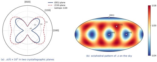
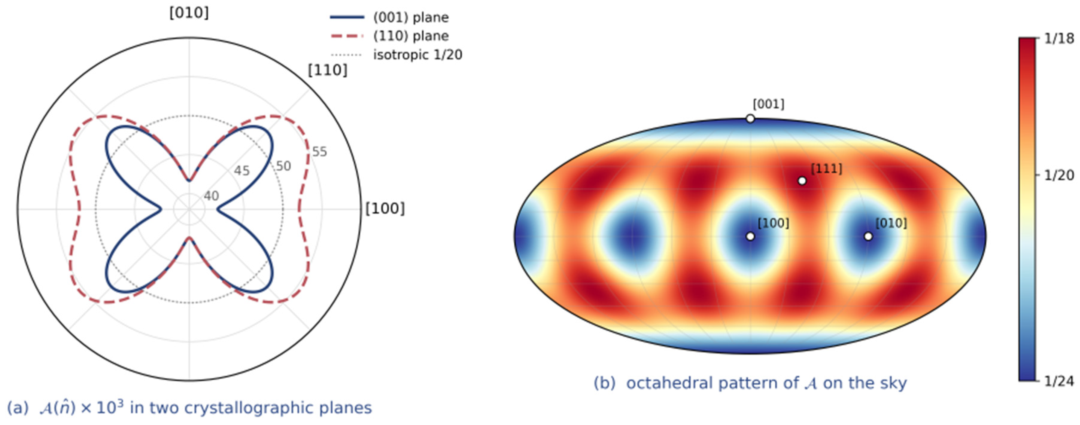

Disclaimer/Publisher’s Note: The statements, opinions and data contained in all publications are solely those of the individual author(s) and contributor(s) and not of MDPI and/or the editor(s). MDPI and/or the editor(s) disclaim responsibility for any injury to people or property resulting from any ideas, methods, instructions or products referred to in the content. |
© 2026 by the author. Licensee MDPI, Basel, Switzerland. This article is an open access article distributed under the terms and conditions of the Creative Commons Attribution (CC BY) license.