Exact Confidence Intervals in Distributions with One Parameter

Abstract

The Clopper–Pearson method of constructing a confidence interval for the probability of success in a binary population that follows a Bernoulli distribution is well known. This paper pedagogically justifies the Clopper–Pearson method and extends the method to all distributions with one parameter whose cumulative probability distribution functions are monotonically continuous with respect to their single parameter. The conservativeness of Clopper–Pearson confidence intervals is proved analytically. Clopper–Pearson confidence intervals are constructed for Poisson, geometric, non-central hyper-geometric, and exponential, etc. It turns out that such extensions result in various well-known confidence intervals in the literature.

1. Introduction

Clopper and Pearson [1] constructed a confidence interval, often called the exact confidence interval, for the probability of success in a binary population that follows a Bernoulli distribution. Among many methods of construction, exact or approximate, the Clopper–Pearson method has been regarded as a golden standard despite its conservativeness, i.e., the actual coverage probability of a Clopper–Pearson confidence interval for any fixed parameter value is at least as high as the nominal confidence level. Exact confidence intervals such as Clopper–Pearson are usually conservative and longer, while approximate confidence intervals such as Wilson and Agresti-Coull are usually less conservative and shorter.

The basic idea of Clopper–Pearson intervals is that an observed value of the statistic, the total number of successes, which follows a binomial distribution, should be an unusual observation for any value of the success probability outside its confidence interval, where unusual observations are those that are no more or no less than the observed value. Because of such an accessible idea, Clopper–Pearson confidence intervals have been included in most statistics textbooks and have been implemented in most statistical software packages.

The literature on confidence intervals for population proportion is extensive. Agresti and Coull [2] compared the true coverage probabilities of approximate confidence intervals such as Wald and Wilson or the score with that of Clopper–Pearson and proposed modified Wald confidence intervals that have coverage probabilities close to the nominal confidence level. Brown et al. [3] reviewed the erratic behaviors of Wald confidence intervals and provided a number of alternative approximate confidence intervals. McGrath et al. [4] assessed the performance of both approximate and Clopper–Pearson confidence intervals in the context of rare events. Schilling and Doi [5] studied optimal confidence intervals by minimizing average length while maximizing coverage probabilities among all length-minimizing procedures. Thulin [6] quantified the cost of using the Clopper–Pearson confidence interval in terms of the increased expected interval length and the increased sample size required to achieve the desired expected length.

However, the pedagogical justification for the Clopper–Pearson method is not available in the literature. The purpose of this paper is twofold. One is to justify the Clopper–Pearson method pedagogically and prove its conservativeness analytically. The other is to extend the Clopper–Pearson method to all distributions with one parameter whose cumulative probability distribution functions are monotonically continuous with respect to their single parameter. We provide extensions of the Clopper–Pearson method to distributions such as Poisson, geometric, non-central hyper-geometric, and exponential, etc. It turns out that such extensions result in various confidence intervals in the literature.

The paper is structured as follows. Section 2 defines and justifies the Clopper–Pearson interval. Results from the literature are reformulated in this section for pedagogical reasons and completion. Extensions of the Clopper–Pearson interval to other distributions are presented in Section 3. Theorem 1 and Corollary 1 lay the foundation of extensions and are not available in the literature. Section 4 provides some concluding remarks.

2. Clopper–Pearson Confidence Interval

Let $X_1$, $X_2$, ⋯, and $X_n$ be independently and identically distributed as Bernoulli distribution with success probability $\pi \in [0,1]$ and $Y={\displaystyle \sum _{i=1}^n}{X}_i$. Note that Y is a sufficient and complete statistic for $\pi$ and follows a binomial distribution with known n and unknown parameter $\pi$, i.e., $Y\sim BIN(n,\pi )$. Clopper and Pearson [1] constructed a two-sided confidence interval of $\pi$ based on the following idea: An observation $y\in \{0,1,\cdots ,n\}$ of Y should be an unusual observation for any $\pi$ outside its confidence interval, i.e., for any $\pi$ outside its $100(1-\alpha )\%$ confidence interval,

$$P[Y\ge y|\pi ]\le {\displaystyle \frac{\alpha }{2}}\mathrm{or}P[Y\le y|\pi ]\le {\displaystyle \frac{\alpha }{2}}.$$

Definition 1. 

Let $X_1$, $X_2$, ⋯, and $X_n$ be independently and identically distributed as Bernoulli distribution with success probability $\pi \in [0,1]$ and $Y={\displaystyle \sum _{i=1}^n}{X}_i$. A $100(1-\alpha )\%$ two-sided Clopper–Pearson confidence interval of π is $({\pi }_l,{\pi }_u)$, where ${\pi }_l$ and ${\pi }_u$ are numerically determined by $P[Y\ge y|{\pi }_l]={\displaystyle \frac{\alpha }{2}}$ and $P[Y\le y|{\pi }_u]={\displaystyle \frac{\alpha }{2}}$, respectively, for $y=1,2,\cdots ,n-1$.

If $y=0$, ${\pi }_l=0$ because $P[Y\ge 0|{\pi }_l]=1$ and ${\pi }_u=1-\sqrt[n]{{\displaystyle \frac{\alpha }{2}}}$ because $P[Y\le 0|{\pi }_u]=P[Y=0|{\pi }_u]={(1-{\pi }_u)}^n$. If $y=n$, ${\pi }_l=\sqrt[n]{{\displaystyle \frac{\alpha }{2}}}$ because $P[Y\ge n|{\pi }_l]=P[Y=n|{\pi }_l]={\pi }_l^n$ and ${\pi }_u=1$ because $P[Y\le n|{\pi }_u]=1$.

For $Y\sim BIN(n,\pi )$, $P[Y\le y|{\pi }_u]$ is not continuous and therefore not a differentiable function of y. However, $P[Y\le y|{\pi }_u]$ is differentiable with respect to $\pi$ for $0<\pi <1$. Lemma 1 next justifies the method of Clopper–Pearson confidence intervals. Ramsey [7] provided a detailed proof and a simplified proof is given below for completeness.

Lemma 1. 

  Suppose that $Y\sim BIN(n,\pi )$ for $\pi \in [0,1]$.

(a). For $y=1,2,\cdots ,n-1$, $P[Y\le y|\pi ]$ is continuous and strictly decreasing for $\pi \in [0,1]$.

(b). For $y=1,2,\cdots ,n-1$, and $0<\alpha <1$, there exist ${\pi }_l$ and ${\pi }_u$ such that ${\pi }_l\le {\pi }_u$ and $P[{\pi }_l<\pi <{\pi }_u]\ge 1-\alpha$, where ${\pi }_l$ and ${\pi }_u$ are unique solutions to $P[Y\ge y|\pi ]={\displaystyle \frac{\alpha }{2}}$ and $P[Y\le y|\pi ]={\displaystyle \frac{\alpha }{2}}$, respectively.

Proof. 

(a) is attained by noting ${\displaystyle \frac{dP[Y\le y|\pi ]}{d\pi }}=-n\left({\displaystyle \genfrac{}{}{0pt}{}{n}{y}}\right){\pi }^y{(1-\pi )}^{(n-1)-y}<0$ for $0<\pi <1$, which can be verified by straightforward differentiation or by the equality

$${\displaystyle \sum _{i=0}^y}\left({\displaystyle \genfrac{}{}{0pt}{}{n}{i}}\right){\pi }^i{(1-\pi )}^{n-i}=(n-y)\left({\displaystyle \genfrac{}{}{0pt}{}{n}{y}}\right){\int }_0^{1-\pi }{t}^{n-y-1}{(1-t)}^{y}dt$$

from integration by parts.

To prove (b), we note that for fixed y, $P[Y\le y|\pi ]$ is continuous and strictly decreasing with respect to $\pi \in [0,1]$, while $P[Y\ge y|\pi ]$ is continuous and strictly increasing for $\pi \in [0,1]$. By the Intermediate Value Theorem in [8], there exist unique ${\pi }_l$ and ${\pi }_u$ such that $P[Y\ge y|\pi ]={\displaystyle \frac{\alpha }{2}}$ and $P[Y\le y|\pi ]={\displaystyle \frac{\alpha }{2}}$, respectively.

Next, we show that ${\pi }_l\le {\pi }_u$ using proof by contradiction. Suppose that ${\pi }_u<{\pi }_l$. Choose some $\pi$ such that ${\pi }_u<\pi <{\pi }_l$. Since $\pi <{\pi }_l$, we have

$$P[Y\ge y|\pi ]<P[Y\ge y|{\pi }_l]={\displaystyle \frac{\alpha }{2}}.$$

Similarly, we have

$$P[Y\le y|\pi ]<P[Y\le y|{\pi }_u]={\displaystyle \frac{\alpha }{2}}$$

because ${\pi }_u<\pi$. Therefore,

$$1=P[0\le Y\le n|\pi ]<P[Y\le y|\pi ]+P[Y\ge y|\pi ]<{\displaystyle \frac{\alpha }{2}}+{\displaystyle \frac{\alpha }{2}}=\alpha ,$$

which contradicts $0<\alpha <1$.

Finally, by construction of the two-sided Clopper–Pearson confidence interval,

$$P[\pi \notin ({\pi }_l,{\pi }_u)]\le P[Y\ge y|\pi \le {\pi }_l]+P[Y\le y|\pi \ge {\pi }_u]\le P[Y\ge y|{\pi }_l]+P[Y\le y|{\pi }_u].$$

Hence,

$$P[{\pi }_l<\pi <{\pi }_u]=1-P[\pi \notin ({\pi }_l,{\pi }_u)]\ge 1-P[Y\ge y|{\pi }_l]-P[Y\le y|{\pi }_u]=1-\alpha .$$

□

In practice, the computation of the Clopper–Pearson interval is usually carried out using the $beta$ or F distributions.

Let $Y\sim BIN(n,\pi )$ and $B(a,b)$ be a random variable with parameters $a>0$ and $b>0$, i.e., $B\sim BETA(a,b)$. Recall that, for $y=0,1,\cdots ,n$,

$${\displaystyle \sum _{i=0}^y}\left({\displaystyle \genfrac{}{}{0pt}{}{n}{i}}\right){\pi }^i{(1-\pi )}^{n-i}=(n-y)\left({\displaystyle \genfrac{}{}{0pt}{}{n}{y}}\right){\int }_0^{1-\pi }{t}^{n-y-1}{(1-t)}^{y}dt$$

$$={\displaystyle \frac{\mathsf{\Gamma }(n+1)}{\mathsf{\Gamma }(n-y)\mathsf{\Gamma }(y+1)}}{\int }_0^{1-\pi }{t}^{n-y-1}{(1-t)}^{y}dt.$$

We have

$$P[Y\le y]=P\left[B\right(n-y,y+1)\le 1-\pi ].$$

Since $1-B(n-y,y+1)=B(y+1,n-y)$, we have

$$P[Y\le y]=1-P\left[B\right(y+1,n-y)\le \pi ].$$

Hence, ${\pi }_u={\mathit{qbeta}}_{1-{\displaystyle \frac{\alpha }{2}},y+1,n-y}$, where ${qbeta}_{1-{\displaystyle \frac{\alpha }{2}},y+1,n-y}$ is the $(1-{\displaystyle \frac{\alpha }{2}})$-quantile of beta distribution with parameters $y+1$ and $n-y$.

On the other hand, since

$$P[Y\ge y]=1-P[Y\le y-1]=1-P\left[B\right(n-y+1,y)\le 1-\pi ]$$

$$=1-P\left[B\right(y,n-y+1)\ge \pi ]=P\left[B\right(y,n-y+1)\le \pi ],$$

We have ${\pi }_l={qbeta}_{{\displaystyle \frac{\alpha }{2}},y,n-y+1}$, where ${qbeta}_{{\displaystyle \frac{\alpha }{2}},y,n-y+1}$ is the ${\displaystyle \frac{\alpha }{2}}$-quantile of beta distribution with parameters y and $n-y+1$.

Note that, if $B(a,b)\sim BETA(a,b)$, ${\displaystyle \frac{bB(a,b)}{a(1-B(a,b\left)\right)}}\sim F(2a,2b)$ for $a>0$ and $b>0$. Hence,

$$1-{\displaystyle \frac{\alpha }{2}}=P[B(y+1,n-y)\le \pi ]=P\left[{\displaystyle \frac{(n-y)B(y+1,n-y)}{(y+1)(1-B(y+1,n-y\left)\right)}}\le {\displaystyle \frac{n-y}{y+1}}{\displaystyle \frac{\pi }{1-\pi }}\right].$$

Therefore,

$${\pi }_u={\displaystyle \frac{(y+1)F_{1-\frac{\alpha }{2},2(y+1),2(n-y)}}{n-y+(y+1)F_{1-\frac{\alpha }{2},2(y+1),2(n-y)}}}$$

$$={\left[1+{\displaystyle \frac{n-y}{(y+1)F_{1-\frac{\alpha }{2},2(y+1),2(n-y)}}}\right]}^{-1},$$

where $F_{p,{\nu }_1,{\nu }_2}$ is the p-quantile of the F distribution with ${\nu }_1$ and ${\nu }_2$ degrees of freedom for $0<p<1$, ${\nu }_1>0$, and ${\nu }_2>0$. Similarly,

$${\displaystyle \frac{\alpha }{2}}=P[B(y,n-y+1)\le \pi ]=P\left[{\displaystyle \frac{(n-y+1)B(y,n-y+1)}{y(1-B(y,n-y+1\left)\right)}}\le {\displaystyle \frac{n-y+1}{y}}{\displaystyle \frac{\pi }{1-\pi }}\right].$$

Therefore,

$${\pi }_l={\displaystyle \frac{y{F}_{\frac{\alpha }{2},2y,2(n-y+1)}}{n-y+1+y{F}_{\frac{\alpha }{2},2y,2(n-y+1)}}}={\left[1+{\displaystyle \frac{n-y+1}{y{F}_{\frac{\alpha }{2},2y,2(n-y+1)}}}\right]}^{-1}.$$

3. Extensions of Clopper–Pearson Confidence Interval

Theorem 1 and and Corollary 1 next extend the Clopper–Pearson interval to any distribution with a cumulative probability distribution that is continuous and monotonic with respect to its single parameter.

Theorem 1. 

  Let $F(y;\theta )$ be the cumulative probability distribution function of a random variable Y for $a\le \theta \le b$, where a and b are real numbers. For any observed value of Y, say, $y_0$, and $0<\alpha <1$, suppose that $F(y_0;\theta )$ is a continuous and decreasing function of $\theta \in [a,b]$, $F(y_0;b)\le {\displaystyle \frac{\alpha }{2}}$, and $F(y_0-;a)\ge 1-{\displaystyle \frac{\alpha }{2}}$, there exist ${\theta }_l$ and ${\theta }_u$ such that ${\theta }_l\le {\theta }_u$ and a two-sided $100(1-\alpha )\%$ Clopper–Pearson confidence interval of θ based on the observation of $y_0$ is $({\theta }_l,{\theta }_u)$, where ${\theta }_u$ is a solution to $F(y_0;\theta )={\displaystyle \frac{\alpha }{2}}$ and ${\theta }_l$ is a solution to $1-F(y_0-;\theta )={\displaystyle \frac{\alpha }{2}}$ or $F(y_0-;\theta )=1-{\displaystyle \frac{\alpha }{2}}$ with $F(y_0-;\theta )=\underset{y\to y_0-}{lim}F(y;\theta )$. If $F(y_0;\theta )>{\displaystyle \frac{\alpha }{2}}$ for all $\theta \in [a,b]$, take ${\theta }_u=b$. If $F(y_0-;\theta )<1-{\displaystyle \frac{\alpha }{2}}$ for $\theta \in [a,b]$, take ${\theta }_l=a$.

A $100(1-\alpha )\%$ upper Clopper–Pearson confidence bound of θ based on the observation $y_0$ is ${\theta }_u$, where ${\theta }_u$ is a solution to $F(y_0;\theta )=\alpha$ if $F(y_0;b)\le \alpha$. If $F(y_0;\theta )>\alpha$ for all $\theta \in [a,b]$, take ${\theta }_u=b$.

Similarly, a $100(1-\alpha )\%$ lower Clopper–Pearson confidence bound of θ based on the observation $y_0$ is ${\theta }_l$, where ${\theta }_l$ is a solution to $F(y_0-;\theta )=1-\alpha$ if $F(y_0-;a)\le 1-\alpha$. If $F(y_0-;\theta )>1-\alpha$ for all $\theta \in [a,b]$, take ${\theta }_l=a$.

Proof. 

We prove the case of two-sided confidence interval and the proofs of lower and upper confidence bounds are similar.

The existence of ${\theta }_l$ and ${\theta }_u$ in the two-sided confidence interval are attained by applying the Intermediate Value Theorem directly. We prove ${\theta }_l\le {\theta }_u$ using proof by contradiction. Suppose that ${\theta }_l>{\theta }_u$. Choose some $\theta$ such that ${\theta }_u<{\theta }_0<{\theta }_l$. Since ${\theta }_u<{\theta }_0$, ${\displaystyle \frac{\alpha }{2}}=F(y_0;{\theta }_u)\ge F(y_0;{\theta }_0)$ because $F(y_0;\theta )$ is decreasing. Note that $F(y_0-;\theta )=\underset{t\to y_0-}{lim}F(y;\theta )$. We know that $F(y_0-;\theta )$ is decreasing and $F(y_0-;{\theta }_0)\ge F(y_0-;{\theta }_l)=1-{\displaystyle \frac{\alpha }{2}}$. Therefore,

$$1\le P[Y\le y_0]+P[Y\ge y_0]=F(y_0;{\theta }_0)+1-F(y_0-;{\theta }_0)\le {\displaystyle \frac{\alpha }{2}}+{\displaystyle \frac{\alpha }{2}}=\alpha ,$$

which contradicts $0<\alpha <1$.

To see that the confidence level of $({\theta }_l,{\theta }_u)$ is at least $100(1-\alpha )\%$, note that

$$P[\theta \notin ({\theta }_l,{\theta }_u)]\le P[Y\ge y_0|\theta \le {\theta }_l]+P[Y\le y_0|\theta \ge {\theta }_u]\le P[Y\ge y_0|{\theta }_l]+P[Y\le y_0|{\theta }_u],$$

we have

$$P[{\theta }_l<\theta <{\theta }_u]=1-P[\theta \notin ({\theta }_l,{\theta }_u)]\ge 1-P[Y\ge y_0|{\theta }_l]-P[Y\le y_0|{\theta }_u]=1-\alpha .$$

□

When the cumulative probability distribution function $F(y;\theta )$ is a continuous and increasing function of $\theta \in [a,b]$, we have the following corollary. We omit the proof of Corollary 1 because it is similar to that of Theorem 1.

Corollary 1. 

  Let $F(y;\theta )$ be the cumulative probability distribution function of a random variable Y for $a\le \theta \le b$, where a and b are real numbers. For any observed value of Y, say, $y_0$, and $0<\alpha <1$, suppose that $F(y_0;\theta )$ is a continuous and increasing function of $\theta \in [a,b]$, $F(y_0;a)\le {\displaystyle \frac{\alpha }{2}}$, and $F(y_0-;b)\ge 1-{\displaystyle \frac{\alpha }{2}}$. There exist ${\theta }_l$ and ${\theta }_u$ such that ${\theta }_l\le {\theta }_u$ and a two-sided $100(1-\alpha )\%$ Clopper–Pearson confidence interval of θ based on the observation of $y_0$ is $({\theta }_l,{\theta }_u)$, where ${\theta }_l$ is a solution to $F(y_0;\theta )={\displaystyle \frac{\alpha }{2}}$ and ${\theta }_u$ is a solution to $1-F(y_0-;\theta )={\displaystyle \frac{\alpha }{2}}$ or $F(y_0-;\theta )=1-{\displaystyle \frac{\alpha }{2}}$. If $F(y_0;\theta )>{\displaystyle \frac{\alpha }{2}}$ for all $\theta \in [a,b]$, take ${\theta }_l=a$. If $F(y_0-;\theta )<1-{\displaystyle \frac{\alpha }{2}}$ for $\theta \in [a,b]$, take ${\theta }_u=b$.

A $100(1-\alpha )\%$ upper Clopper–Pearson confidence bound of θ based on the observation $y_0$ is ${\theta }_u$, where ${\theta }_u$ is a solution to $F(y_0;\theta )=1-\alpha$ if $F(y_0-;\theta )\le 1-\alpha$. If $F(y_0-;\theta )>1-\alpha$ for all $\theta \in [a,b]$, take ${\theta }_u=b$.

Similarly, a $100(1-\alpha )\%$ lower Clopper–Pearson confidence bound of θ based on the observation $y_0$ is ${\theta }_l$, where ${\theta }_l$ is a solution to $F(y_0;\theta )=\alpha$ if $F(y_0;a)\le \alpha$. If $F(y_0;\theta )>\alpha$ for all $\theta \in [a,b]$, take ${\theta }_l=a$.

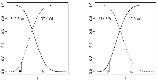
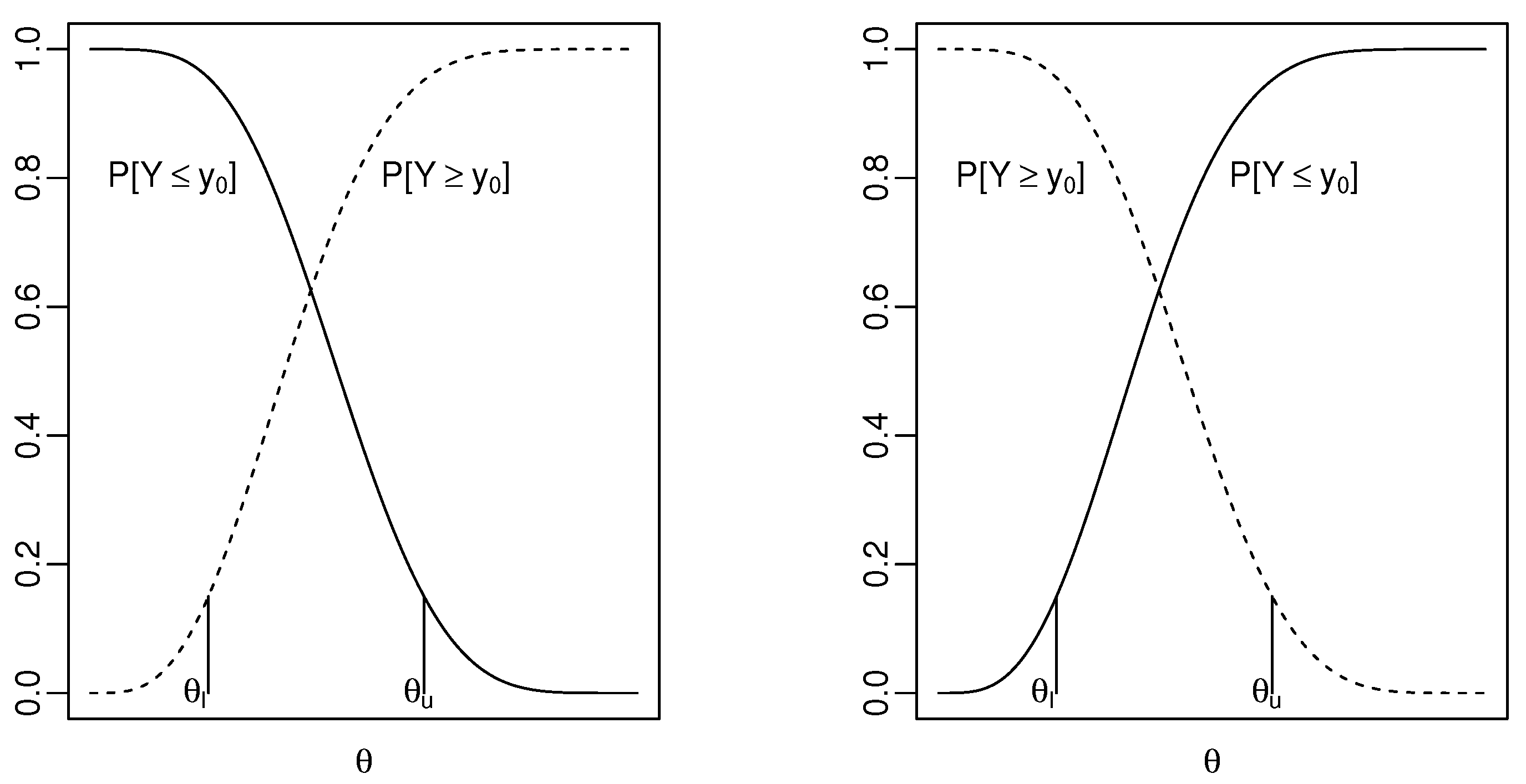
Figure 1 on the next page graphically displays the idea of Theorem 1 and Corollary 1 where solid lines are $P[Y\le y_0]$ as functions of $\theta$ and dashed lines are $P[Y\ge y_0]$ as functions of $\theta$.

Figure 1. Clopper–Pearson confidence intervals.

Remark 1. 

For a discrete or continuous random variable Y, the strictly monotonic property of $F(y_0;\theta )$ results in the uniqueness of ${\theta }_l$ and ${\theta }_u$ in the confidence intervals or confidence bounds.

Remark 2. 

The conclusions of Theorem 1 hold when $F(y_0;\theta )$ is a continuous and monotonic function of $\theta \in (a,b)$ and both $\underset{\theta \to b-}{lim}F(y_0;\theta )$ and $\underset{\theta \to a+}{lim}F(y_0;\theta )$ exist and are finite. In fact, let $F^{*}(y_0;\theta )=F(y_0;\theta )$ for $\theta \in (a,b)$, $F^{*}(y_0;b)=\underset{\theta \to b-}{lim}F(y_0;\theta )$, and $F^{*}(y_0;a)=\underset{\theta \to a+}{lim}F(y_0;\theta )$ and the results are obtained by applying Theorem 1 to $F^{*}(y_0;\theta )$.

Remark 3. 

Not every cumulative probability distribution function with one parameter is monotonic function of the parameter for any y in its domain. Consider a normal distribution with mean $\theta >0$ and variance ${\theta }^2$. Its cumulative probability distribution function $\mathsf{\Phi }\left({\displaystyle \frac{y}{\theta }}-1\right)$ is strictly increasing for $y<0$ and strictly decreasing for $y>0$, where $\mathsf{\Phi }(·)$ is the cumulative probability distribution function of the standard normal distribution.

Since the lower and upper $100(1-\alpha )\%$ confidence bounds are the lower and upper limits of the $100(1-2\alpha )\%$ two-sided confidence interval, respectively, we only construct two-sided confidence intervals in the following.

• Extension to Poisson distribution: Let $X_1$, $X_2$, ⋯, and $X_n$ be independently and identically distributed as Poisson distribution with parameter $\lambda$. Let $Y={\displaystyle \sum _{i=1}^n}{X}_i$. Note that Y is a sufficient and complete statistic for $\lambda$ and follows a Poisson distribution $POI\left(n\lambda \right)$.  

Let $\mu =n\lambda$. Consider the cumulative probability distribution function of Y, $F(y;\mu )=P[Y\le y]={\displaystyle \sum _{k=0}^y}{\displaystyle \frac{{\mu }^k}{k!}}{e}^{-\mu }$. It is straightforward to show that ${\displaystyle \frac{dF(y;\mu )}{d\mu }}=-{\displaystyle \frac{{\mu }^y}{y!}}<0$. Therefore, $F(y;\mu )$ is a continuous and strictly decreasing function of $\mu$ for any fixed $y\ge 0$. Note that $F(y;0)=1$ and $\underset{\mu \to \infty }{lim}F(y;\mu )=0$ for any fixed $y\ge 0$.

Through integration by parts, we have ${\displaystyle \sum _{k=0}^y}{\displaystyle \frac{{\mu }^k}{k!}}{e}^{-\mu }={\displaystyle \frac{1}{y!}}{\int }_{\mu }^{\infty }{t}^y{e}^{-t}dt$. Therefore, $P[Y\le y]=P\left[G\right(y+1,1)\ge \mu ]$, which is a continuous and strictly decreasing function of $\mu$ for fixed $y\ge 0$. $P[Y\ge y]=1-P[Y\le y-1]=P\left[G\right(y,1)\le \mu ]$, where $G(y,1)$ is a random variable that has a gamma distribution with shape parameter y and scale parameter 1.

A two-sided $100(1-\alpha )\%$ Clopper–Pearson type confidence interval for $\mu$ is $({\mu }_l,{\mu }_u)$, where ${\mu }_l=qgamm{a}_{{\displaystyle \frac{\alpha }{2}},y,1}$, ${\mu }_u=qgamm{a}_{1-{\displaystyle \frac{\alpha }{2}},y+1,1}$, and $qgamm{a}_{p,a,b}$ is the p-quantile of gamma distribution with shape parameter a and scale parameter b for $0<p<1$, $a>0$, and $b>0$. Therefore, a two-sided $100(1-\alpha )\%$ Clopper–Pearson type confidence interval for $\lambda$ is $({\lambda }_l,{\lambda }_u)$, where ${\lambda }_l=qgamm{a}_{{\displaystyle \frac{\alpha }{2}},y,1}/n$ and ${\lambda }_u=qgamm{a}_{1-{\displaystyle \frac{\alpha }{2}},y+1,1}/n$ for $y\ge 0$.

Recall that $G(y,1)={\displaystyle \frac{1}{2}}{\chi }_{2y}^2$, ${\lambda }_l={\chi }_{{\displaystyle \frac{\alpha }{2}},2y}^2/\left(2n\right)$ and ${\lambda }_u={\chi }_{1-{\displaystyle \frac{\alpha }{2}},2(y+1)}^2/\left(2n\right)$, where ${\chi }_{p,\nu }^2$ is the p-quantile of chi-square distribution with $\nu$ degrees of freedom for $0<p<1$ and $\nu >0$. These are the fiducial limits proposed by Garwood [9]. Agresti and Coull [2] mentioned this idea of constructing the exact confidence interval for $\mu$ but no details were given. Patil and Kulkarni [10] compared the Garwood interval with other eighteen intervals in terms of coverage probability and expected length.

• Extension to geometric distribution: Let $X_1$, $X_2$, ⋯, $X_n$ be independently and identically distributed as a geometric distribution with success probability $\pi$, i.e., $P[X=x]=\pi {(1-\pi )}^x$, for $x=0,1,\cdots$, and $0<\pi <1$ and $Y={\displaystyle \sum _{i=1}^n}{X}_i$. Note that Y is a sufficient and complete statistic for $\pi$ and follows a negative binomial distribution, i.e., $Y\sim NB(n,\pi )$.  

In order to show the cumulative probability distribution function of the negative binomial distribution is a continuous and strictly increasing function of $\pi$, we need Lemma 2, which is first proved in [11]. We modified Rider’s proof next to make the presentation more comprehensible.

Lemma 2. 

  Suppose that $Y\sim NB(n,\pi )$ for $\pi \in [0,1]$.

(a). For any integer $y\ge 1$, $P[Y\ge y|\pi ]$ is a continuous and strictly decreasing function of $\pi \in [0,1]$. Therefore, $P[Y\le y|\pi ]$ is a continuous and strictly increasing function of $\pi \in [0,1]$.

(b). For any integer $y\ge 1$, $P[Y\le y|\pi ]=P[B(n,y+1)\le \pi ]$, where $B(n,y+1)$ is a random variable that has a beta distribution with parameters n and $y+1$.

Proof. 

To prove (a), consider $P[Y\ge y|\pi ]={\displaystyle \sum _{k=y}^{\infty }}\left({\displaystyle \genfrac{}{}{0pt}{}{k+n-1}{k}}\right){\pi }^n{(1-\pi )}^k$. For $t>0$, let $\pi ={\displaystyle \frac{1}{t+1}}$. $1-\pi ={\displaystyle \frac{t}{1+t}}$. For any integer $y\ge 1$,

$$P[Y\ge y|t]={\displaystyle \sum _{k=y}^{\infty }}\left({\displaystyle \genfrac{}{}{0pt}{}{k+n-1}{k}}\right){\displaystyle \frac{t^k}{{(1+t)}^{k+n}}}.$$

$${\displaystyle \frac{dP[Y\ge y|t]}{dt}}={\displaystyle \sum _{k=y}^{\infty }}{\displaystyle \frac{(n+k-1)!}{k!(n-1)!}}\left[{\displaystyle \frac{k{t}^{k-1}}{{(1+t)}^{n+k}}}-{\displaystyle \frac{(n+k)t^k}{{(1+t)}^{n+k+1}}}\right]$$

$$={\displaystyle \sum _{k=y-1}^{\infty }}{\displaystyle \frac{(n+k)!}{k!(n-1)!}}{\displaystyle \frac{t^k}{{(1+t)}^{n+k+1}}}-{\displaystyle \sum _{k=y}^{\infty }}{\displaystyle \frac{(n+k)!}{k!(n-1)!}}{\displaystyle \frac{t^k}{{(1+t)}^{n+k+1}}}$$

$$={\displaystyle \frac{(n+y-1)!}{(y-1)!(n-1)!}}{\displaystyle \frac{t^{y-1}}{{(1+t)}^{n+y}}}>0.$$

Therefore, $P[Y\ge y|\pi ]$ is a continuous and strictly decreasing function of $\pi \in [0,1]$.

For (b), since $P[Y\ge y|t]=0$ when $t=0$ for any $y\ge 1$, we have

$$P[Y\ge y|t]={\int }_0^t{\displaystyle \frac{dP[Y\ge y]}{ds}}ds={\displaystyle \frac{(y-1)!(n-1)!}{(n+y-1)!}}{\int }_0^t{s}^{y-1}{(1+s)}^{-n-y}ds.$$

Let $u={\displaystyle \frac{1}{s+1}}$,

$$P[Y\ge y|t]={\displaystyle \frac{(y-1)!(n-1)!}{(n+y-1)!}}{\int }_{{\displaystyle \frac{1}{t+1}}}^1{u}^{n-1}{(1-u)}^{y-1}du$$

$$={\displaystyle \frac{(y-1)!(n-1)!}{(n+y-1)!}}{\int }_{\pi }^1{u}^{n-1}{(1-u)}^{y-1}du.$$

Therefore, $P[Y\ge y|\pi ]=P[B(n,y)\ge \pi ]$, where $B(n,y)$ is a random variable that has a beta distribution with parameters n and y. Hence, $P[Y\le y|\pi ]=1-P[Y\ge y+1\left|\pi \right]=1-P\left[B\right(n,y+1)\ge \pi ]=P\left[B\right(n,y+1)\le \pi ]$.    □

Since $P[Y\le y]$ is a continuous and strictly increasing function of $\pi$ when $Y\sim NB(n,\pi )$, a two-sided $100(1-\alpha )\%$ confidence interval of Clopper–Pearson type for $\pi$ is $({\pi }_l,{\pi }_u)$, where ${\pi }_l={qbeta}_{{\displaystyle \frac{\alpha }{2}},n,y+1}$, ${\pi }_u=qbet{a}_{1-{\displaystyle \frac{\alpha }{2}},n,y}$, and ${qbeta}_{p,a,b}$ is the p-quantile of a beta distribution with shape parameters a and b for $0<p<1$, $a>0$, and $b>0$. When $y=0$, $P[Y\le 0|\pi ]=P[Y=0|\pi ]={\pi }^n$ and $P[Y\ge y|\pi ]=1$. Hence, ${\pi }_l=\sqrt[n]{{\displaystyle \frac{\alpha }{2}}}$ and ${\pi }_u=1$.

• Extension to noncentral hypergeometric distribution: Let $X\sim BIN(n_x,{\pi }_x)$, $Y\sim BIN(n_y,{\pi }_y)$, X, and Y be independent. The conditional distribution of $X|X+Y=t$ for $t\ge 0$ is Fisher’s noncentral hypergeometric distribution. For $max\{0,t-n_y\}\le x\le min\{t,n_x\}$,

  $$\begin{array}{cc}\hfill & P[X=x|X+Y=t]={\displaystyle \frac{P[X=x,X+Y=t]}{P[X+Y=t]}}={\displaystyle \frac{P[X=x,Y=t-x]}{P[X+Y=t]}}\hfill \\ \hfill & ={\displaystyle \frac{\left(\genfrac{}{}{0pt}{}{n_x}{x}\right){\pi }_x^x{(1-{\pi }_x)}^{n_x-x}\left(\genfrac{}{}{0pt}{}{n_y}{t-x}\right){\pi }_y^{t-x}{(1-{\pi }_y)}^{n_y-(t-x)}}{{\displaystyle \sum _{u=max\{0,t-n_y\}}^{min\{t,n_x\}}}\left(\genfrac{}{}{0pt}{}{n_x}{u}\right){\pi }_x^u{(1-{\pi }_x)}^{n_x-u}\left(\genfrac{}{}{0pt}{}{n_y}{t-u}\right){\pi }_y^{t-u}{(1-{\pi }_y)}^{n_y-(t-u)}}}\hfill \\ \hfill & ={\displaystyle \frac{\left(\genfrac{}{}{0pt}{}{n_x}{x}\right){\left(\frac{{\pi }_x}{1-{\pi }_x}\right)}^x{(1-{\pi }_x)}^{n_x}\left(\genfrac{}{}{0pt}{}{n_y}{t-x}\right){\left(\frac{{\pi }_y}{1-{\pi }_y}\right)}^{t-x}{(1-{\pi }_y)}^{n_y}}{{\displaystyle \sum _{u=max\{0,t-n_y\}}^{min\{t,n_x\}}}\left(\genfrac{}{}{0pt}{}{n_x}{u}\right){\left(\frac{{\pi }_x}{1-{\pi }_x}\right)}^x{(1-{\pi }_x)}^{n_x}\left(\genfrac{}{}{0pt}{}{n_y}{t-u}\right){\left(\frac{{\pi }_y}{1-{\pi }_y}\right)}^{t-x}{(1-{\pi }_y)}^{n_y}}}\hfill \\ \hfill & ={\displaystyle \frac{\left(\genfrac{}{}{0pt}{}{n_x}{x}\right)\left(\genfrac{}{}{0pt}{}{n_y}{t-x}\right){\psi }^x}{{\displaystyle \sum _{u=max\{0,t-n_y\}}^{min\{t,n_x\}}}\left(\genfrac{}{}{0pt}{}{n_x}{u}\right)\left(\genfrac{}{}{0pt}{}{n_y}{t-u}\right){\psi }^u}},\hfill \end{array}$$

  where $\psi =\left({\displaystyle \frac{{\pi }_x}{1-{\pi }_x}}\right)/\left({\displaystyle \frac{{\pi }_y}{1-{\pi }_y}}\right)={\displaystyle \frac{{\pi }_x(1-{\pi }_y)}{{\pi }_y(1-{\pi }_x)}}$ is the odds ratio.  

To construct a $100(1-\alpha )\%$ confidence interval for $\psi$, we need the following Lemma 3 to show that the cumulative probability distribution function of the noncentral hypergeometric distribution is a continuous and strictly decreasing function of $\psi$ in $(0,\infty )$.

Lemma 3. 

Let $P\left(x\right)=a_0+a_{1}x+\cdots +a_n{x}^n$ be a polynomial of x of order $n\ge 1$ with all positive coefficients $a_i$. For any $0\le m<n$, let $Q\left(x\right)={\displaystyle \frac{a_0+a_{1}x+\cdots +a_m{x}^m}{P\left(x\right)}}$. Then, $Q\left(x\right)$ is a continuous and strictly decreasing function of x in $(0,\infty )$, $Q\left(0\right)=1$, and $\underset{x\to \infty }{lim}Q\left(x\right)=0$.

The proof of Lemma 3 is straightforward and is omitted. It can also be derived as a special case of the Appendix of [12].

For any $t\ge 0$, let $W_t=X|X+Y=t$ where $X\sim BIN(n_x,{\pi }_x)$, $Y\sim BIN(n_y,{\pi }_y)$, X and Y are independent. By Lemma 3 the cumulative probability distribution function of $W_t$, $P[W_t\le w]$, is a continuous and strictly decreasing function of $\psi$ for $0<\psi <\infty$ and $max\{0,t-n_y\}\le w\le min\{t,n_x\}$. Therefore, a two-sided $100(1-\alpha )\%$ confidence interval for $\psi$ is $({\psi }_l,{\psi }_u)$ where ${\psi }_l$ and ${\psi }_u$ are unique solutions to $P[W_t\ge w|{\psi }_l]={\displaystyle \frac{\alpha }{2}}$ and $P[W_t\le w|{\psi }_u]={\displaystyle \frac{\alpha }{2}}$,, respectively, for $max\{0,t-n_y\}<w<min\{t,n_x\}$. If $w=max\{0,t-n_y\}$, ${\psi }_l=0$ because $P[W_t\ge max\{0,t-n_y\}|\psi ]=1$. If $w=min\{t,n_x\}$, ${\psi }_u=\infty$ because $P[W_t\le min\{t,n_x\}|\psi ]=1$.

The two-sided $100(1-\alpha )\%$ Clopper–Pearson confidence interval is the inversion of the two-sided central Fisher’s exact test in [13] by using the exact conditional tails. Since there are no explicit formulas for ${\psi }_l$, and ${\psi }_u$, an R [14] function using MCMCpack package [15] has been written for the numerical computation of the two-sided confidence interval and is given in Appendix A.

Example 1. 

Fay [13] presented a study of CCR5 deficiency due to infection with West Nile virus. Among 15 subjects who were homozygous for CCR5 deficiency, 4 subjects had abdominal pain, while 50 had abdominal pain among 619 subjects who were heterozygous for CCR5 deficiency. The sample odds ratio of abdominal pain from homozygous subjects to heterozygous subjects is about $4.14$. The $95\%$ Clopper–Pearson confidence interval for the population odds ratio is $(0.92,14.58)$, which is wider than the corresponding Wald interval $(1.27,13.47)$, the Fay exact interval $(1.17,14.17)$ in [13], and Blaker’s exact interval $(1.17,14.22)$ in [16]. Moreover, since 1 is in the Clopper–Pearson interval but not in other intervals, the population proportions of abdominal pain among homozygous and heterozygous patients are not statistically different based on the Clopper–Pearson interval, but they are statistically different based on Wald approximate interval, Blaker, and Fay exact intervals.

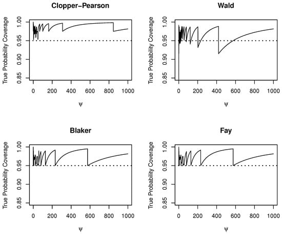
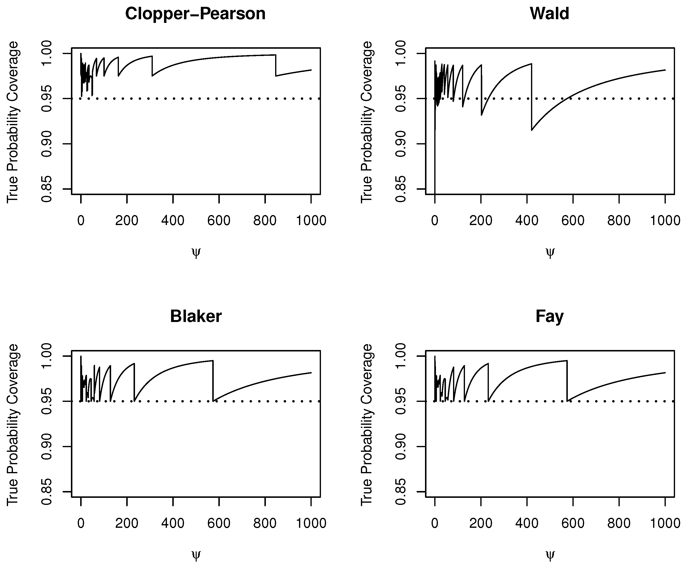
Figure 2 displays the true probability coverage of the four confidence intervals of the $95\%$ confidence level. The conservativeness of the Clopper–Pearson interval over the Blaker and Fay exact intervals and the insufficient probability coverage of the Wald interval are apparent.

Figure 2. True Probability Coverage of Clopper–Pearson, Wald, Blaker, and Fay Intervals.

• Extension to exponential distribution: Let $X_1$, $X_2$, ⋯, and $X_n$ be independently and identically distributed as an exponential distribution with parameter $\lambda >0$ or $EXP\left(\lambda \right)$, i.e., $f\left(x\right)=\lambda e^{-\lambda x}$ for $x>0$. Note that $Y={\displaystyle \sum _{i=1}^n}{X}_i$ is a sufficient and complete statistic for $\lambda$ and $2\lambda Y\sim {\chi }_{2n}^2$ because $2\lambda X_i\sim {\chi }_2^2$. For any observed value of Y, say, y, $P[Y\le y]=P[2\lambda Y\le 2\lambda y]=F_{{\chi }_{2n}^2}\left(2\lambda y\right)$, where $F_{{\chi }_{2n}^2}(·)$ is the cumulative probability distribution function of ${\chi }_{2n}^2$.  

Since $F_{{\chi }_{2n}^2}\left(2\lambda y\right)$ is a continuous and strictly increasing function of $\lambda$, $F_{{\chi }_{2n}^2}\left(0\right)=0$ and $\underset{\lambda \to \infty }{lim}{F}_{{\chi }_{2n}^2}\left(2\lambda y\right)=1$, a two-sided $100(1-\alpha )\%$ Clopper–Pearson confidence interval is $({\lambda }_l,{\lambda }_u)$, where ${\lambda }_l$ is the unique solution to $F_{{\chi }_{2n}^2}\left(2\lambda y\right)={\displaystyle \frac{\alpha }{2}}$ and ${\lambda }_u$ is the unique solution to $F_{{\chi }_{2n}^2}\left(2\lambda y\right)=1-{\displaystyle \frac{\alpha }{2}}$, i.e., ${\lambda }_l={\chi }_{{\displaystyle \frac{\alpha }{2}},2n}^2/\left(2y\right)$ and ${\lambda }_u={\chi }_{1-{\displaystyle \frac{\alpha }{2}},2n}^2/\left(2y\right)$, where ${\chi }_{p,\nu }^2$ is the p-quantile of chi-square distribution with degrees of freedom $\nu$ for $0<p<1$ and $\nu >0$. This two-sided confidence interval is exactly the same as the one obtained by the method of pivotal quantity with pivotal quantity $2\lambda Y$, i.e., $P[{\chi }_{{\displaystyle \frac{\alpha }{2}},2n}^2<2\lambda Y<{\chi }_{1-{\displaystyle \frac{\alpha }{2}},2n}^2]=1-\alpha$.

Recall the relationship between the exponential distribution and the two-parameter Weibull distribution when the shape parameter is known; we construct a Clopper–Pearson type of confidence interval for the rate parameter as follows. Consider a random sample $X_1$, $X_2$, ⋯, and $X_n$ from a two-parameter Weibull distribution with shape parameter $k>0$ and rate parameter $\beta >0$, i.e., the probability density function is $f(x;k,\beta )=k{\beta }^k{x}^{k-1}{e}^{-{\left(\beta x\right)}^k}$, for $x\ge 0$. When k is known, a sufficient statistic for $\beta$ is $Y={\displaystyle \sum _{i=1}^n}{X}_i^k$. Since $X_i^k\sim EXP\left({\beta }^k\right)$, $2{\beta }^k{X}_i^k\sim {\chi }_2^2$ and $2{\beta }^{k}Y\sim {\chi }_{2n}^2$. For any observed value of Y, say, y, $P[Y\le y]=P[2{\beta }^{k}Y\le 2{\beta }^{k}y]=F_{{\chi }_{2n}^2}\left(2{\beta }^{k}y\right)$, where $F_{{\chi }_{2n}^2}(·)$ is the cumulative probability distribution function of ${\chi }_{2n}^2$.

Since $F_{{\chi }_{2n}^2}\left(2{\beta }^{k}y\right)$ is a continuous and strictly increasing function of $\beta$, $F_{{\chi }_{2n}^2}\left(0\right)=0$ and $\underset{\beta \to \infty }{lim}{F}_{{\chi }_{2n}^2}\left(2{\beta }^{k}y\right)=1$, a two-sided $100(1-\alpha )\%$ Clopper–Pearson confidence interval of $\beta$ is $({\beta }_l,{\beta }_u)$, where ${\beta }_l$ is the unique solution to $F_{{\chi }_{2n}^2}\left(2{\beta }^{k}y\right)={\displaystyle \frac{\alpha }{2}}$ and ${\beta }_u$ is the unique solution to $F_{{\chi }_{2n}^2}\left(2{\beta }^{k}y\right)=1-{\displaystyle \frac{\alpha }{2}}$, i.e., ${\beta }_l=\sqrt[k]{{\chi }_{{\displaystyle \frac{\alpha }{2}},2n}^2/\left(2y\right)}$ and ${\beta }_u=\sqrt[k]{{\chi }_{1-{\displaystyle \frac{\alpha }{2}},2n}^2/\left(2y\right)}$, where ${\chi }_{p,\nu }^2$ is the p-quantile of chi-square distribution with $\nu$ degrees of freedom for $0<p<1$ and $\nu >0$.

Note that the Rayleigh distribution with scale parameter $\sigma$ and probability density function $f(x;\sigma )={\displaystyle \frac{x}{{\sigma }^2}}{e}^{-{\displaystyle \frac{x^2}{2{\sigma }^2}}}$ is a special Weibull distribution with shape parameter $k=2$ and rate parameter $\beta ={\displaystyle \frac{1}{\sigma \sqrt{2}}}$. A two-sided $100(1-\alpha )\%$ Clopper–Pearson confidence interval of $\sigma$ based on a random sample $X_1$, ⋯, and $X_n$ from the Rayleigh distribution is $\left(\sqrt{{\displaystyle \sum _{i=1}^n}{x}_i^2/{\chi }_{1-{\displaystyle \frac{\alpha }{2}},2n}^2},\sqrt{{\displaystyle \sum _{i=1}^n}{x}_i^2/{\chi }_{{\displaystyle \frac{\alpha }{2}},2n}^2}\right)$.

The following two extensions are from [17] and were presented there as examples of fiducial confidence intervals. Since fiducial confidence intervals are not very comprehensible among statistical practitioners, we represent them next as Clopper–Pearson confidence intervals.

• Extension to normal distribution: Let $X_1$, $X_2$, ⋯, $X_n$ be independently and identically distributed as a normal distribution with unknown mean $\mu$ and known standard deviation $\sigma$, i.e., $N(\mu ,{\sigma }^2)$. The sample mean $\overline{X}={\displaystyle \frac{1}{n}}{\displaystyle \sum _{i=1}^n}{X}_i$ is a sufficient and complete statistic for $\mu$. For any observed value of $\overline{X}$, say, $\overline{x}$, consider ${\displaystyle \frac{\alpha }{2}}=P[\overline{X}\le \overline{x}]=P\left[{\displaystyle \frac{\sqrt{n}\overline{X}-\mu }{\sigma }}\le {\displaystyle \frac{\sqrt{n}(\overline{x}-\mu )}{\sigma }}\right]=\mathsf{\Phi }\left({\displaystyle \frac{\sqrt{n}(\overline{x}-\mu )}{\sigma }}\right)$ and $1-{\displaystyle \frac{\alpha }{2}}=P[\overline{X}>\overline{x}]=\mathsf{\Phi }\left({\displaystyle \frac{\sqrt{n}(\mu -\overline{x})}{\sigma }}\right)$, where $\mathsf{\Phi }(·)$ is the cumulative probability distribution function of $N(0,1)$. Since $\mathsf{\Phi }\left({\displaystyle \frac{\sqrt{n}(\overline{x}-\mu )}{\sigma }}\right)$ is a continuous and strictly decreasing function of $\mu$, $\underset{\mu \to -\infty }{lim}\mathsf{\Phi }\left({\displaystyle \frac{\sqrt{n}(\overline{x}-\mu )}{\sigma }}\right)=1$, and $\underset{\mu \to \infty }{lim}\mathsf{\Phi }\left({\displaystyle \frac{\sqrt{n}(\overline{x}-\mu )}{\sigma }}\right)=0$, the two-sided $100(1-\alpha )\%$ Clopper–Pearson confidence interval is $(\overline{x}-z_{1-{\displaystyle \frac{\alpha }{2}}}{\displaystyle \frac{\sigma }{\sqrt{n}}},\overline{x}+z_{1-{\displaystyle \frac{\alpha }{2}}}{\displaystyle \frac{\sigma }{\sqrt{n}}})$, where $z_{1-{\displaystyle \frac{\alpha }{2}}}$ is the $(1-{\displaystyle \frac{\alpha }{2}})$-quantile of standard normal distribution. This two-sided Clopper–Pearson confidence interval is exactly the same as the one obtained by the method of pivotal quantity.
• Extension to uniform distribution: Let $X_1$, $X_2$, ⋯, $X_n$ be independently and identically distributed as a uniform distribution on $(0,\theta )$ for $\theta >0$. Note that $Y=max\{X_1,X_2,\cdots ,X_n\}$ is a sufficient and complete statistic for $\theta$.  

For any observed value of Y, say, y, $P[Y\le y]={\left({\displaystyle \frac{y}{\theta }}\right)}^n={\displaystyle \frac{\alpha }{2}}$ and $P[Y\ge y]=1-{\left({\displaystyle \frac{y}{\theta }}\right)}^n={\displaystyle \frac{\alpha }{2}}$. Since $P[Y\le y]$ is a continuous and strictly decreasing function of $\theta$ on $(y,\infty )$, $\underset{\theta \to y}{lim}P[Y\le y]=1$, and $\underset{\theta \to \infty }{lim}P[Y\le y]=0$, the two-sided $100(1-\alpha )\%$ Clopper–Pearson confidence interval is $\left({\displaystyle \frac{y}{\sqrt[n]{1-\frac{\alpha }{2}}}},{\displaystyle \frac{y}{\sqrt[n]{\frac{\alpha }{2}}}}\right)$.

Although we have extended the Clopper–Pearson method to some continuous distributions above, it seems that the most popular way to construct confidence intervals for continuous distributions in practice is the method of the pivotal quantity.

4. Conclusions

We have pedagogically justified the Clopper–Pearson method in constructing confidence intervals for the success probability of a binary population that follows a Bernoulli distribution and extended the method to all distributions with one parameter whose cumulative probability distribution functions are monotonically continuous with respect to their single parameter. These extensions expand the applications of the Clopper–Pearson method extensively. One attractive feature of Clopper–Pearson confidence intervals is their conservativeness, i.e., their true coverage probabilities are at least as high as their nominal levels. We prove such conservativeness analytically. Due to such conservativeness, Clopper–Pearson confidence intervals are widely applied in quality control and clinical trials where conservative decision-making is needed. Compared with other exact intervals such as Blaker and Fay, the cost quantification of the conservativeness of the Clopper–Pearson confidence interval in terms of the increased expected length and the increased sample size makes it more appealing to practitioners.

Although we focus on two-sided confidence intervals of equal tails in this paper, unequal-tailed two-sided confidence intervals can be constructed similarly.

References

- Clopper, C.; Pearson, E.S. The use of confidence or fiducial limits illustrated in the case of the binomial. Biometrika 1934, 26, 404–413. [Google Scholar] [CrossRef]
- Agresti, A.; Coull, B.A. Approximate is better than “Exact” for interval estimation of binomial proportions. Am. Stat. 1998, 52, 119–126. [Google Scholar] [CrossRef] [Scilit]
- Brown, L.D.; Cai, T.T.; DasGupta, A. Interval estimation for a binomial proportion. Stat. Sci. 2001, 16, 101–133. [Google Scholar] [CrossRef] [Scilit]
- McGrath, O.; Burke, K. Binomial Confidence intervals for rare events: Importance of defining margin of error relative to magnitude of proportion. Am. Stat. 2024, 78, 437–449. [Google Scholar] [CrossRef] [Scilit]
- Schilling, M.F.; Doi, J.A. A coverage probability approach to finding an optimal binomial confidence procedure. Am. Stat. 2014, 68, 133–145. [Google Scholar] [CrossRef] [Scilit]
- Thulin, M. The cost of using exact confidence intervals for a binomial proportion. Electron. J. Stat. 2014, 8, 817–840. [Google Scholar] [CrossRef] [Scilit]
- Ramsey, L.T. (Traditional) Exact Confidence Intervals for the Binomial Distribution. Available online: https://www.math.hawaii.edu/~ramsey/TraditionalBinomialCI.pdf (accessed on 5 February 2025).
- Stewart, J.; Clegg, D.; Watson, S. Calculus, Early Transcendentals, 9th ed.; Cengage Learning: Boston, MA, USA, 2021; p. 122. [Google Scholar]
- Garwood, F. Fiducial Limits for the Poisson Distribution. Biometrika 1936, 28, 437–442. [Google Scholar] [CrossRef] [Scilit]
- Patil, V.V.; Kulkarni, V.H. Comparison of confidence intervals for the Poisson mean: Some new aspects. REVSTAT-Stat. J. 2012, 10, 211–227. [Google Scholar]
- Rider, P.R. The negative binomial distribution and the incomplete beta function. Am. Math. Mon. 1962, 69, 302–304. [Google Scholar] [CrossRef] [Scilit]
- Mehta, C.R.; Patel, N.R.; Gray, R. Computing an exact confidence interval for the common odds ratio in several 2 × 2 contingency tables. J. Am. Stat. Assoc. 1985, 80, 969–973. [Google Scholar] [CrossRef] [Scilit]
- Fay, M.P. Confidence intervals that match Fisher’s exact or Blaker’s exact tests. Biostatistics 2010, 11, 373–374. [Google Scholar] [PubMed]
- R Core Team. A Language and Environment for Statistical Computing R Foundation for Statistical Computing; R Foundation for Statistical Computing: Vienna, Austria, 2026. [Google Scholar]
- Martin, A.D.; Quinn, K.M.; Park, J.H. MCMCpack: Markov Chain Monte Carlo in R. J. Stat. Softw. 2011, 42, 1–21. [Google Scholar] [CrossRef] [Scilit]
- Blaker, H. Confidence curves and improved exact confidence intervals for discrete distributions. Can. J. Stat. 2000, 28, 783–798. [Google Scholar] [CrossRef] [Scilit]
- Wang, Y.H. Fiducial intervals: What are they? Am. Stat. 2000, 54, 105–111. [Google Scholar] [CrossRef] [Scilit]
Disclaimer/Publisher’s Note: The statements, opinions and data contained in all publications are solely those of the individual author(s) and contributor(s) and not of MDPI and/or the editor(s). MDPI and/or the editor(s) disclaim responsibility for any injury to people or property resulting from any ideas, methods, instructions or products referred to in the content. |
© 2026 by the author. Licensee MDPI, Basel, Switzerland. This article is an open access article distributed under the terms and conditions of the Creative Commons Attribution (CC BY) license.