


Abstract
The Shapley value is the predominant point-valued solution concept in cooperative game theory and has recently become a foundational method in interpretable machine learning. In this domain, a prevailing strategy for circumventing the computational intractability of exact Shapley values is to approximate them via a weighted least squares optimization framework. In this paper, we investigate an existing algorithmic framework for weighted least squares Shapley approximation, assessing its feasibility for feature attribution. Methodologically, we conduct a theoretical variance analysis within a Monte Carlo sampling framework, investigate an approach for sample reuse across strata, and establish a relation to Unbiased KernelSHAP. Our analysis reveals three main findings: (i) a structural equivalence between least squares sampling and Unbiased KernelSHAP; (ii) the non-zero covariance between sampled coalitions introduced by reusing samples across strata in one of the existing least squares-based approaches; and (iii) the absence of a universally optimal sampling strategy across tasks. We validate these results empirically on several cooperative games and practical machine learning problems.
1. Introduction
The original KernelSHAP paper by Lundberg and Lee [1] from 2017 was a landmark success for interpretable machine learning. Its primary achievement was making the Shapley value [2]—a theoretically optimal but computationally intractable [3,4,5] concept from cooperative game theory [6]—practical for explaining machine learning models. Lundberg and Lee [1] discovered that the exact Shapley values for a prediction could be recovered as the solution to a specially weighted least squares regression problem. By sampling a manageable number of coalitional inputs and solving this approximate regression, KernelSHAP provided a single, consistent metric for feature importance. The accompanying open-source library SHAP [1] fueled its widespread use, making it a predominant standard for model interpretation, particularly in the model-agnostic setting.
The follow-up work on Unbiased KernelSHAP by Covert and Lee [7] represents a success in strengthening methodological rigor. It addresses the problem that the original KernelSHAP algorithm has not been proven to be unbiased, does not provide uncertainty estimates, and offers no finite-sample error guarantees, making it difficult to assess the reliability of its explanations in practice. While not as publicly visible as the initial breakthrough, this refinement solidified SHAP’s foundation as a robust, statistically sound tool. Despite these advances, KernelSHAP (and to a lesser extent, its unbiased variant) still leaves several methodological questions open: the original algorithm lacks unbiasedness and uncertainty quantification, and neither variant provides explicit guidance on how to choose the number of samples to achieve a desired precision. These gaps motivate the search for alternative estimators with clearer theoretical properties.
According to Lundberg and Lee [1], KernelSHAP was developed without knowledge of prior articles on cooperative game theory like Charnes et al. [8] and Ruiz et al. [9], who decades earlier had already derived the precise weighting scheme that makes a least squares regression yield the Shapley value when complete data is available. This outlines a fascinating case of parallel innovation across disciplines. Cooperative game theory, with the Shapley value [2] as its most important solution concept, had long been a mature and applied field providing rigorous solutions to real-world problems of fair division and coalitional analysis, from allocating airport landing fees among airlines based on runway use [10] to measuring the voting power of political blocs in a legislature [11,12,13]. Yet, the field of machine learning, increasingly reliant on inscrutable black-box models, had not seen its own predictions as precisely such a system—where input features act as cooperating agents whose joint effort produces a model’s output. Lundberg and Lee’s pivotal contribution [1] was to bridge this conceptual gap. They recognized that the abstract “game” defined by a model’s prediction function was a natural domain for Shapley’s theory. By doing so, they inadvertently reinvented a specific computational tool—the weighted least squares approximation—from the game theory literature, but with a transformative new purpose: not to analyze economic coalitions, but to explain the inner logic of artificial intelligence.
Whereas KernelSHAP [1] and its unbiased variant [7] are widely used, the methods from Benati et al. [14]—which are equally based on the least squares formulation of the Shapley value—have received comparatively little attention. This article represents, to the best of our knowledge, their first application in explainable artificial intelligence. We adapt the ideas from Benati et al. [14] as general TU game approximation algorithms, terming their weighted sampling strategy LSS (least squares sampling). Regarding their proposal for stratification, we differentiate S-LSS (no sample reuse across strata) from SRS-LSS (with sample reuse), while noting that both stratification schemes introduce theoretical complications that we specify in detail below. However, the framework by Benati et al. [14] itself has received little critical examination. Its stratified estimators (S-LSS and SRS-LSS) are presented without formal variance analysis or finite-sample guarantees, and the practical implications of their overlapping strata and sample reuse remain unexplored. Thus, while these methods are theoretically elegant, their strengths and weaknesses relative to KernelSHAP and UKS are not well understood. Consequently, the following theoretical questions remain unresolved: (i) Under what conditions does stratification reduce variance, and does S-LSS guarantee such a reduction? (ii) How does sample reuse across strata affect the covariance structure of SRS-LSS? (iii) What is the exact relationship between LSS and UKS, and why do their theoretical Hoeffding bounds differ? (iv) How tight are these finite-sample bounds in practice? These questions are not merely academic: without answers, practitioners cannot predict which algorithm will perform well on a given problem, nor can they rely on finite-sample guarantees for the least squares-based methods. Moreover, the relationship between the approach by Benati et al. [14] and the widely used KernelSHAP family remains opaque, hindering informed method selection.
The objective of this paper is to address these open questions by providing a detailed structural, theoretical, and algorithmic analysis of the methods LSS, S-LSS, and SRS-LSS from Benati et al. [14]. In contrast to prior work, we do not propose a new estimator but rather clarify the properties of existing ones, resolving the ambiguities listed above. Specifically, our research question is as follows: What are the structural relationships between the least squares-based Shapley value approximation algorithms proposed by Benati et al. [14] (LSS, S-LSS, SRS-LSS) and the widely used KernelSHAP and Unbiased KernelSHAP (UKS)? These strategies differ fundamentally: KernelSHAP estimates both the regression matrix and the target vector from samples, whereas UKS precomputes the exact matrix. LSS uses a single importance sampling distribution over all coalitions, while S-LSS and SRS-LSS introduce player- and size-dependent sampling schemes.
This article does the following:
- Compares the variances of LSS and S-LSS in detail, showing that S-LSS is not a valid stratified estimator in the classical sense and that neither algorithm dominates the other.
- Points out how sample reuse across strata may introduce non-zero covariance terms between strata for SRS-LSS, making its theoretical analysis difficult.
- Proves that LSS and UKS approximate the same underlying problem, thereby only differing in their respective sampling strategies, which explains why their empirical performance is often similar despite different theoretical bounds.
- Derives finite-sample bounds for LSS, UKS, and S-LSS and then critically assesses their tightness and practical relevance through numerical experiments in Section 6.
- Tests how the unbiased Shapley estimators LSS, S-LSS, and SRS-LSS compare with KernelSHAP and UKS for both classical cooperative games and real-world applications from interpretable machine learning.
The remainder of this article is structured as follows. In Section 2, we summarize basic ideas from cooperative game theory, including linear solution concepts and the Shapley value, and introduce the BShap (Baseline Shapley) model for interpretable machine learning. Section 3 briefly reviews Monte Carlo methods, along with stratified sampling and importance sampling for variance reduction. A summary of results on approximating linear solution concepts by means of importance sampling on the coalition space from our previous work [15] is presented in Section 4. The central developments of this paper are detailed in Section 5, where we formally introduce the LSS, S-LSS, and SRS-LSS estimators and elaborate on the first three contributions outlined above: the variance comparison between LSS and S-LSS, the analysis of non-zero covariances in SRS-LSS, and the formal proof of structural equivalence between LSS and UKS. In addition, we derive finite-sample Hoeffding bounds for LSS, UKS, and S-LSS. The empirical performance of all algorithms—including a critical assessment of these bounds—is analyzed in Section 6 using two types of cooperative games and three real-world explainability scenarios, thereby numerically substantiating our previous analytical claims. The paper concludes in Section 7 with a summary and recommendations.
2. Preliminaries on Cooperative Game Theory, the Shapley Value and the BShap Model for Interpretable Machine Learning
Following the expositions in Chakravarty et al. [6], Peters [16], and Benati et al. [14], this section offers a concise introduction to transferable utility (TU) cooperative games and point-valued solution concepts such as the Shapley value. Additionally, we briefly describe two representative TU games—the airport game and the weighted voting game—and the model from interpretable machine learning that we utilize in our analysis and our numerical experiments in Section 6.
2.1. Transferable Utility Games and Their Characteristic Functions
We investigate transferable utility games (TU games), cooperative games where a coalition’s earnings are expressed as a scalar [6,16]. This implies that the utility can be distributed without restriction among the players.
Following [6,16], a TU game is formally defined as a pair . Here, is the player set and is the characteristic function, which assigns a real value to each coalition representing its total utility from cooperation. We adopt the standard normalization .
It is frequently convenient to represent a coalition S by an indicator vector . We define and its inverse . This mapping allows functions and operators defined on or to be used interchangeably; for instance, and denote the same value, and .
2.2. Linear Solution Concepts for TU Games
Let denote the set of all TU games on player set N. A point-valued solution concept is a function that returns a vector for each game . Each entry quantifies the value assigned to player i. These concepts are employed to evaluate individual influence or to distribute a coalition’s payoff among its members .
A key property of a point-valued solution concept is linearity [14]. This requires that can be written as
with ⊙ denoting the Hadamard product of vectors, standing for weights depending only on S and the player, and denoting values depending upon S, v, and the player.
2.3. The Shapley Value
The Shapley value [2] represents the most prominent solution concept in cooperative game theory. In recent years, it has been extensively adopted in machine learning and explainable artificial intelligence [1,17,18,19]. Formally, for any player , the Shapley value is the expected marginal contribution , taken over all sets S of players that precede i in a uniformly random permutation of N, i.e.,
where denotes a uniform distribution, the set of all permutations of N, and the set of players preceding i in a permutation .
Let be the vector of Shapley values, and let represent any approximation, with denoting its i-th entry. Where no ambiguity arises, we use to denote .
It follows directly from (3) that the Shapley value belongs to the class of linear solution concepts introduced in Section 2.2. The coefficients are specified by and
Note that the Shapley value exhibits symmetry, i.e., two players that contribute equally to each coalition have the same Shapley value, meaning we have
for any game and any players with . It also exhibits efficiency, i.e., for all games it holds that .
2.4. Airport Games
Airport games, proposed by Littlechild and Thompson [10], address the problem of distributing runway construction costs among players whose aircraft require different runway lengths. Costs are encoded in a vector , where corresponds to player i. The characteristic function is
Classified as line-graph maintenance problems, these games have closed-form Shapley values [20], making them ideal benchmark instances for the numerical studies in Section 6.
2.5. Weighted Voting Games
Weighted voting games [6,16,21] represent voting bodies in which players possess different voting weights (e.g., parliamentary seats), collected in . A coalition S succeeds when for a predetermined quota C. This yields a characteristic function defined by
In our theoretical and numerical investigations in Section 5 and Section 6, we frequently use a family of weighted voting games with players and
There exist fast methods for computing point-valued solutions of weighted voting games for a number of players, for instance, dynamic programming algorithms [22,23]. Hence, these games serve as excellent test games for our experiments in Section 6.
2.6. Baseline Shapley (BShap) for Interpretable Machine Learning
Our numerical experiments in Section 6 apply the Shapley value framework to attribute a model’s prediction to its input features. Here, the prediction task is interpreted as a cooperative game with features as players. Given a model and an input , the characteristic function specifies the value of a feature subset S.
We adopt Baseline Shapley (BShap), a method originally suggested by [1] and formalized by Sundararajan and Najmi [24]. The value is defined deterministically relative to a single baseline vector , where features not in S are set to their baseline counterparts:
with denoting the set of features not in S. The subtrahend in (8) ensures the normalization as introduced in Section 2.1. Note that this normalization would not be needed for the algorithms based on marginal contributions investigated in our article [15], but becomes crucial for the algorithms based on least squares formulations of the Shapley value discussed in Section 5.
Our specific baseline: In the applications in Section 6, the baseline is taken as the expected feature vector over the training distribution:
with representing the training data distribution. This anchors Shapley values to the prediction of an average sample, providing a natural reference point. The resulting attributions thus explain the deviation of from this baseline.
3. Preliminaries on Monte Carlo Methods for Estimation
In this section, we first introduce the use of Monte Carlo methods for estimating expectations together with two variance reduction techniques. We draw mainly from the short overviews provided by Rubinstein and Kroese [25] and Botev and Ridder [26] as well as from the textbook by Rubinstein and Kroese [27].
Let be a d-dimensional discrete (or continuous) random variable with a sample space and a probability mass function (or probability density function, respectively), which may be known or unknown. Denote a specific realization of by . For a function , we want to estimate the expectation
This expectation is frequently intractable in closed form, either because is unknown (and only i.i.d. samples are given) or because the defining sum or integral is computationally infeasible. Monte Carlo methods circumvent this analytical hurdle through simulation.
We begin with Crude Monte Carlo as the foundational method, then present importance sampling and stratified sampling for variance reduction, which we examine in this paper. A finite variance of is assumed throughout this manuscript.
3.1. Crude Monte Carlo Method
Crude Monte Carlo proceeds by drawing an i.i.d. sample and averaging the values. This yields the standard estimator [26]:
According to [26], the estimator is unbiased, i.e., , and its variance is
3.2. Stratified Sampling for Variance Reduction
Stratified sampling is a well-established Monte Carlo variance reduction technique [26]. It separates the sample space into ℓ disjoint strata such that with for . Suppose L is a discrete random variable taking values in with known probabilities . We can rewrite as
with denoting the expectation over the conditional probability distribution of given that . Our stratified estimator of becomes
where denotes the estimated value of in stratum , i.e.,
with the sample of size being drawn i.i.d. from the conditional probability distribution of given that . To ensure fair comparisons to other Monte Carlo techniques, we always assume (up to rounding errors), where denotes the overall sample budget. The estimator is unbiased [26], i.e.,
Assuming that the sample sizes per stratum are proportionally assigned, i.e., , the variance of the crude Monte Carlo estimator (11) has been established as an upper bound [26], i.e.,
meaning that the stratified estimator never performs worse than its crude counterpart .
3.3. Importance Sampling for Variance Reduction
Importance sampling introduces another probability mass (or density) function , such that . This allows (9) to be rewritten as
A Monte Carlo approximation based on (13) is
where . As shown in [25], this estimator is unbiased, i.e., , and its variance is analogous to the crude Monte Carlo case
With a properly selected , the variance of the importance sampling estimator is less than or equal to that of the crude Monte Carlo estimator. This follows from comparing (11) and (15), yielding
which holds because can always be chosen as the trivial case. We apply importance sampling in the context of TU games in Section 4.
4. Approximating Linear Solution Concepts via Importance Sampling
The exact calculation of a linear solution concept, i.e., (1), for a TU game normally requires summing up terms whose number grows exponentially in the number of players, n. Therefore, approximation algorithms are needed to estimate these values in real-world situations, especially in the context of applications in interpretable machine learning [1,17,18,19] where one typically cannot exploit any special structure of the underlying game for computing Shapley values exactly. In this section, we briefly summarize some ideas from [14] and the general framework for importance sampling on the coalition space for linear solution concepts, which we recently proposed in [15] and will apply in Section 5.
Benati et al. [14] consider a uniform sampling strategy on the coalition space for approximating linear solution concepts, i.e., they simply adopt the uniform distribution . Let us regard it as the crude Monte Carlo method on the coalition space. Although sampling subsets from the uniform distribution is both straightforward and unbiased, it is obviously not an optimal—or even recommended—sampling strategy for all linear solution concepts or problem settings. For example, when approximating the Shapley value by sampling coalitions using (3), small or large coalitions obtain larger weights, resulting in a strong influence on the estimator. However, when sampling uniformly from the coalition space, they may extract only a few samples, resulting in a less accurate estimator.
To enable more efficient sampling, we apply the importance sampling technique from Section 3.3. By appropriately reweighting the estimator, importance sampling allows us to draw samples from a non-uniform, user-defined distribution while maintaining an unbiased estimate of the underlying linear solution concept.
Theorem 1
([15]). For all , let
be a probability distribution and with be a sample of size τ generated by sampling with replacement according to . Then,
is an importance sampling estimator of the linear solution concept .
The following proposition connects our importance sampling estimator from Theorem 1 established in Pollmann and Staudacher [15] to a finding from Benati et al. [14], p. 95.
Proposition 1.
The importance sampling estimator from Theorem 1 has the following properties:
- (a)
- It is unbiased, i.e.,
- (b)
- Its variance is given by
- (c)
- It is consistent in probability, i.e.,
We note that Theorem 1 and Proposition 1 subsume both the crude Monte Carlo method (setting ) and stratified sampling. The latter is covered because any stratum estimator for a linear solution concept can be written in the form of (16), allowing direct application of these results.
5. Least Squares Approaches for Approximating Shapley Values
This section covers the approach of approximating Shapley values as a least squares problem. First, we give an introduction to the family of least square values in Section 5.1, followed by an overview of Shapley value approximation algorithms in this setting in Section 5.2. In Section 5.3, Section 5.4, Section 5.5 and Section 5.6, we compare these algorithms and put them into the overall context.
5.1. The Family of Least Square Values
The family of least square values was proposed by Ruiz et al. [9] and comprises a generalization of the formulation of the Shapley value as a least squares problem, which was already proposed earlier by Charnes et al. [8].
Essentially, this family consists of all solution concepts that can be obtained as minimizers of a weighted least squares problem, where the weights determine the relative importance of different coalition sizes. These weights are given by the function that assigns a weight to each coalition size with for at least one s. Clearly, by definition, m is symmetric in the sense of assigning the same weight to coalitions of the same cardinality in order to retrieve symmetric solutions like the Shapley value. We denote by a payoff vector for a given game, where is the payoff for player i. In the following, we use the shorthand notation . Recall that a payoff vector is called efficient if .
With these definitions established, any solution concept in the family of least square values can be expressed as the optimizer of the following weighted least squares problem:
where m is the weight function that is specific to the particular solution concept.
These expressions illustrate how the resulting allocation depends on the weight function m.
5.1.1. Least Square Values as Linear Solution Concepts
Let us briefly point out why all members of the family of least square values are linear solution concepts in the sense of the definition from Section 2.2. Benati et al. [14] showed that (21) can be rewritten as
where is the all-ones vector and the individual elements of are given by
From (23), it follows directly that this representation satisfies the definition of linear solution concepts provided in Section 2.2.
5.1.2. The Shapley Value in the Context of Least Square Values
The family of least square values was introduced by Ruiz et al. [9] after Charnes et al. [8] had demonstrated that the Shapley value can be expressed as a least squares optimization problem. In detail, the vector of Shapley values is the solution to problem (20) when m is defined as
and therefore, via (22), one obtains
Thus, by inserting (26) into (21) and reformulating the result, one obtains the closed-form solution for the Shapley value as
with given by (22) for all . We illustrate the computation of the Shapley value as a least squares optimization problem in Figure 1.
Figure 1.
Let be a cooperative game with and , , , and . The player 1 and player 2 axes should be interpreted in a discrete way such that 0 denotes the exclusion and 1 specifies the inclusion of a player. The blue plane is the solution to problem (20) with m being defined as (25) and being obtained from (26). As a result, the coefficients defining this plane are the Shapley values of the game , i.e., , and .
5.2. Shapley Value Approximation Algorithms
In this section, we provide an introduction to Shapley value approximation algorithms that are based on the formulation of the Shapley value as a least squares problem. The algorithms discussed below are not meant to be an exhaustive list, but rather represent those algorithms we will analyze and test in the rest of the article. Specifically, the first three algorithms have been proposed by Benati et al. [14] in the context of stochastic approximations of cooperative games and are based on the family of least square values defined in Section 5.1, while the latter two have their origins in the machine learning world.
Additionally, we would like to draw attention to the absence of the projection method proposed by Benati et al. [14], which ensures efficiency and symmetry of the obtained estimators. Although this approach potentially improves the accuracy of the estimators (or at least never makes their accuracy worse), it is not agnostic to the underlying characteristic function, as it requires prior knowledge about symmetric players, which is information that we assume to be unavailable—in particular, in the context of interpretable machine learning. Nevertheless, one could still achieve estimator efficiency through a single evaluation of , similar to Castro et al. [28], who proposed filling the “efficiency gap” post hoc. However, since such additional considerations lie outside the scope of this work, we exclude them from all algorithms equally.
5.2.1. Least Squares Sampling (LSS)
This paragraph deals with an algorithm proposed by Benati et al. [14] that approximates (23) by using importance sampling as defined in Theorem 1. Specifically, we refer to the estimator in Equation (22) on p. 97 in the paper [14] combined with their weighted sampling strategy. In the following, we name this algorithm LSS.
The idea of LSS is to sample coalitions with replacement according to
such that, by combining (24), (25), (26), and (28), one obtains
Then, based on Theorem 1 as well as (23) and (29), an approximation of the Shapley value of player i is given by
where is obtained by sampling times with replacement according to p.
Equation (31) serves as the basis for Algorithm 1. Note that one evaluation of v can be used to update all players, reducing the number of evaluations of v and increasing convergence speed.
| Algorithm 1 LSS |
|
Since (31) is an importance sampling estimator of a linear solution concept in the sense of Theorem 1, which can easily be obtained via (23) and (30), LSS inherits the properties stated in Proposition 1. Thus, the estimator is unbiased, and we can use (18) to calculate its variance:
Proposition 2.
The variance of the LSS estimator is given by
with
for all .
Proof.
Using (18) and setting results in
where . Here, the term is excluded from the variance calculation since it is added once at the beginning of the LSS algorithm, but it is not part of the sampling procedure, and thus, there is no randomness to it, and it does not influence the variance of . As a result, we construct a temporary solution concept of the game, , that does not contain the constant term .
5.2.2. Stratified Least Squares Sampling (S-LSS)
This paragraph discusses another algorithm proposed by Benati et al. [14], which approximates the Shapley value through what the authors introduce as their stratification strategy. Specifically, we refer to Equations (23) and (24) on p. 97 in the paper [14] without any reuse of samples across strata. In the following, we refer to this method as S-LSS.
The stratification according to [14] comes into play when approximating the individual addends in (21), where a reformulation of (22) results in
Based on that formulation, approximations of , denoted by , are obtained as
with being an i.i.d. sample of size from according to the uniform probability distribution .
Then, based on (27), one obtains an estimator of as
forming the basis for Algorithm 2.
| Algorithm 2 S-LSS |
|
Clearly, by using the formulation given in (35), the estimators can be seen as estimators of individual solution concepts in the sense of Theorem 1 by setting
as well as
and .
Therefore, the individual stratum estimators are unbiased, and (18) can be used to calculate their variances:
Proposition 3.
In the context of the S-LSS algorithm, the variance of is given by
for all and .
Proof.
Based on the individual stratum estimator variances given by Proposition 3, Benati et al. [14] stated the overall variance of the estimated Shapley value of player i as
Perhaps surprisingly, and contrary to what might be expected from the definition of stratified sampling in Section 3.2, S-LSS does not guarantee a smaller variance compared with LSS, as we discuss in Section 5.3 and show empirically in Section 6.
5.2.3. Sample Reuse Stratified Least Squares Sampling (SRS-LSS)
Benati et al. [14] proposed a third algorithm, which is based on the S-LSS algorithm and reuses samples across strata. Specifically, we refer to the final three sentences in subsection 4.2 on p. 97 in the paper [14]. In the following, we refer to this method as SRS-LSS.
The central idea is to reuse one evaluation in (35) to update all stratum estimators where and , hence the name. To achieve that, samples of size are drawn from with probabilities . Based on the elements of , all stratum estimators with are updated with a single evaluation . As a side effect, the number of evaluations of v that are used to update player j’s stratum, i.e., , depends on the generated samples, which is why in Algorithm 3, we need to keep track of their values as well. This essentially means that all become estimators themselves, which is why we denote them by . We will characterize their behavior in the following proposition. Additionally, we use to denote unnormalized estimators of before dividing by .
| Algorithm 3 SRS-LSS |
|
Proposition 4.
Let as for all . Then, with probability approaching one asymptotically, each stratum estimator receives at least one sample, i.e.,
Proof.
The probability of a player belonging to a random coalition of size is given by . Thus, we have
Although the probability of an individual being zero converges to zero as the overall sample budget increases, safeguards are needed to ensure that SRS-LSS does not fail in real-world scenarios. A straightforward approach is to repeatedly generate samples until all or to employ a conditional probability distribution that accounts for which elements have not yet been sampled. As an alternative, we implement a warm-up phase (see Algorithm 4) similar to SVARM [30], which ensures that each estimator receives at least one sample. We emphasize that the computational overhead of this warm-up phase is minimal and that this phase uses the same underlying sampling distribution as the main phase of SRS-LSS. For instance, the sample requirements scale modestly with the number of players n, requiring only 250 samples for n = 50, 572 samples for , and 8052 samples for .
Since Benati et al. [14] did not include a variance analysis of the SRS-LSS estimator in their work, we refer to Section 5.4 for a detailed discussion of the variance of the obtained estimator.
| Algorithm 4 WarmUp |
|
5.2.4. KernelSHAP (KS)
Let us now introduce the KernelSHAP algorithm, one of the predominant Shapley approximation algorithms in the machine learning world. It was developed by Lundberg and Lee [1], without knowledge of prior works such as [8,9]. The optimization objective is
to calculate the Shapley values for the cooperative game [7]. Here, denotes a probability mass function satisfying and such that
where
is the Shapley kernel and
is a normalization constant [7]. As noted in Section 2.1, all functions defined on are implicitly also defined on N.
Since solving (40) requires optimizing over the elements in , a set that grows exponentially in n, KernelSHAP approximates Shapley values by generating a sample of size and solving the approximate optimization problem defined over the sampled subsets only, i.e.,
Based on the Lagrangian, Covert and Lee [7] derived the closed-form solution
The resulting estimator is consistent in probability, but assessing its unbiasedness or variance is challenging due to terms like . While the unbiasedness or variance of or can be analyzed individually [7], their interaction complicates the analysis of the final Shapley value estimator.
The KernelSHAP algorithm will not be further analyzed theoretically in this work. Due to its setup, it is unclear how the obtained estimator fits the framework defined by Theorem 1 or Monte Carlo estimators introduced in Section 3 in general. To the best of our knowledge, no analytic solution for its variance or a proof of its unbiasedness has been derived to date, which is why the Unbiased KernelSHAP algorithm was introduced, guaranteeing unbiasedness and facilitating the variance analysis of the obtained Shapley value estimator.
5.2.5. Unbiased KernelSHAP (UKS)
The UKS algorithm [7] is a continued development of the KernelSHAP algorithm from the previous paragraph, where we pointed out that it is unclear if the KernelSHAP estimator is unbiased due to the interactions between and .
Considering the original optimization problem defined in (40), its Lagrangian with multiplier is given by
where Z is a random variable taking values from and is distributed according to p, as defined by (41). With that formulation, the closed-form solution of the original problem can be derived as
Clearly, cannot be computed exactly for large n, since it depends on v, and thus, requires evaluations of v to be exact. Nevertheless, since A does not depend on v and the probability distribution p is known, A can be pre-computed and is exact, which is the main improvement introduced by UKS in contrast to the original KernelSHAP algorithm.
Thus, UKS estimates all players’ Shapley values via
where is defined in (45) as in the KernelSHAP algorithm, i.e., , and is given by
with
Following the results provided in [7], the resulting Shapley value estimator is unbiased and consistent in probability. Furthermore, its covariance is given by
with
and
5.3. Comparison of LSS and S-LSS
In this section, we first clarify the relationship between the two algorithms, LSS and S-LSS, which we introduced at the beginning of Section 5.2, followed by a detailed comparison of variances.
5.3.1. Algorithm Comparison
For comparing the algorithms LSS and S-LSS, we start with the following proposition:
Proposition 5.
In the sense of the definition of stratified sampling provided in Section 3.2, S-LSS is not a valid stratification scheme of LSS.
Proof.
As stated in Section 3.2, stratification divides the sample space into strata , such that for and .
Observing the strata definitions given in (34) shows that their sample spaces intersect as follows:
Clearly, for any coalition size , this set is nonempty, since it contains at least one element of the form , where the dots indicate the presence of distinct players other than j and . Therefore, S-LSS does not form a valid partition of the sample space as required by our definition in Section 3.2. □
We note in passing that the structure of the overlap between strata does not introduce bias into the Shapley estimator defined by S-LSS.
In order to generate a deeper understanding of the relationship between LSS and S-LSS, we explain how Benati et al. [14] derived the LSS algorithm from the initial formulation given by (21). Via (21) and (22), one directly obtains
which matches the formulation proposed in (23) with weights given by (24). Therefore, one evaluation of v for a given S in (51) corresponds to updating all where in (50). This implicit update of all where is encapsulated by the weight function .
As a result, stratifying by s and j, as done in the case of S-LSS, cannot be derived from LSS in the same way as defined in Section 3.2, since LSS is an algorithm that simultaneously updates multiple strata of S-LSS with a single sampled element, i.e., with one evaluation of v.
We conclude that the statement from Section 3.2, which points out that stratified sampling always yields a variance less than or equal to the variance of the crude Monte Carlo method, does not apply here, since S-LSS is not a valid stratification scheme of LSS. Therefore, in order to understand how their variances compare, we calculate both algorithms’ variances on two selected examples.
5.3.2. Variance Comparison in the Absence of Variance Within Strata
First, let us compare the variances of the LSS and S-LSS estimators in the context of an example game characterized by large variance between strata and no variance within strata. In particular, we consider a cardinality game with players and the characteristic function
Lemma 1.
On the game defined by (52) with , the variance of the LSS estimator is greater than zero for all players, i.e.,
Proof.
First, we find that the Shapley values of the game are given by for all , since all i are symmetric. Without loss of generality, we fix one player in order to simplify the notation. Then, using Proposition 2, we derive
Inserting into (32), multiplying by , and using the identities defined by (37) as well as
results in
Dividing by , we obtain
Lemma 2.
On the game defined by (52) with , the variance of the S-LSS estimator is zero for all players, i.e.,
as long as for all and .
Proof.
Without loss of generality, we fix and in order to simplify the notation.
Corollary 1.
There exist games for which the variances of all players’ S-LSS estimators are smaller than those of the corresponding LSS estimators, i.e.,
as long as the sample allocation scheme of S-LSS satisfies for all and .
Proof.
The proof is straightforward and follows directly from Lemmas 1 and 2. □
5.3.3. Variance Comparison in the Presence of Variance Within Strata
Let us now consider a weighted voting game as defined in (6) with
as a second example. Here, we use concrete numbers in order to simplify calculations. In detail, we are interested in the variances of the Shapley value estimators of player 2 with Shapley value .
To simplify our later reasoning, we first calculate the population and estimator variances for all strata of the S-LSS estimator in Table 1.
Table 1.
Population and estimator variances for all strata of the S-LSS estimator.
Lemma 3.
On the game defined by (55), the variance of player 2’s LSS estimator is given by
Lemma 4.
On the game defined by (55), the variance of player 2’s S-LSS estimator with equal sample allocation is given by
Proof.
Corollary 2.
There exist games for which the variance of a player’s S-LSS estimator with equal sample allocation is larger than that of the LSS estimator, i.e., for some .
Proof.
The proof is straightforward and directly follows from Lemmas 3 and 4. □
Although an equal sample allocation scheme might be a reasonable choice, especially when calculating all players’ Shapley values, one might still ask whether alternative allocation procedures could further reduce the variance of the S-LSS estimator. While our goal is to treat characteristic functions—and, in the context of explainable machine learning, the machine learning models behind them—as black boxes without relying on internal knowledge, let us examine a sample allocation strategy that makes use of a priori information about the variances within strata. Interestingly, we will see that even this variance-informed allocation performs worse than the LSS method on the weighted voting game defined by (55).
Lemma 5.
On the game defined by (55), the variance of player 2’s S-LSS estimator with an optimum sample allocation, i.e., a sample allocation that is tailored to player 2 in order to minimize the variance of their estimator, is given by
Proof.
By inserting the estimator variances from Table 1 into (38), we obtain
where is the fraction of that is used for estimating the stratum with and is the fraction of that is used for estimating the stratum with .
Therefore, we get the proxy minimization problem
Let us now set
with its derivative given by
Setting , we get
where is the only solution in . Furthermore, since
we can see that is indeed a minimum with the value Thus, via (56), the minimum variance of the S-LSS estimator is given by
Corollary 3.
There exist games for which the variance of a player’s S-LSS estimator with optimum sample allocation, i.e., a sample allocation that is tailored to that specific player in order to minimize the variance of their estimator, is larger than that of the LSS estimator, i.e., for some .
Proof.
The proof is straightforward and directly follows from Lemmas 3 and 5. □
5.3.4. Concluding Variance Comparison of LSS and S-LSS
Summarizing the results from the previous two paragraphs, we obtain:
Theorem 2.
Depending on the specific cooperative game, the variance of a player’s Shapley value estimator may be smaller under either LSS or S-LSS, even when the S-LSS algorithm uses an optimal, player-specific sample allocation.
Proof.
The proof is straightforward and directly follows from Corollaries 1 and 3. □
To summarize the results in this section so far, Proposition 5 demonstrates that S-LSS is not the stratified variant of LSS in the sense of the definition provided in Section 3.2, and Theorem 2 states that neither algorithm is preferable over the other one on all cooperative games. Since the proof of Theorem 2 builds on the calculation of both algorithms’ theoretical variances on two distinct games, it does not provide an intuitive explanation why S-LSS may perform worse than LSS in some settings. Therefore, we provide an explanation in the following.
Since Benati et al. [14] did not provide a sample allocation scheme for the S-LSS algorithm, we first derive a proportional sample allocation similar to Section 3.2, which is motivated by the fact that all coalition sizes are equally likely in the context of LSS, i.e.,
with , where is the probability mass function from (28).
Furthermore, once a random coalition of some size is sampled, the probability of any player being in it is the same for all players, i.e.,
Then, the overall probability that a random coalition belongs to a specific stratum of the S-LSS algorithm—which is the case when meets a specific size s and, additionally, some specific player j is in it—is given by
As we established at the beginning of this section, the statement on variance reduction for a stratified estimator with stratum sample sizes proportional to the probabilities of sampled elements belonging to a stratum from Section 3.2 does not apply in this context since S-LSS is not a valid stratified variant of LSS. However, the proportional sample allocation turns out to be a useful starting point for our subsequent explanations. Moreover, as established in Theorem 2, the exact choice of the applied sample allocation scheme does not alter the fact that S-LSS can perform worse than LSS, since the increased variance of S-LSS was also observed under an optimal allocation scheme. Additionally, as we will show later, sample allocation strategies other than the proportional sample allocation do not change the outcome and conclusions of our following reasoning.
Hence, we set all . Then, we obtain
On the other hand, let us now find out how often a sample is expected to belong to a stratum of S-LSS when actually running LSS, which is denoted by . Via (57), we obtain
Finally, by comparing (58) and (59), we observe
for all and . Clearly, (60) shows that the expected sample size for stratum is larger by a factor of when executing LSS compared with the corresponding sample size of S-LSS with a proportional sample allocation. This is due to the fact that LSS actually updates multiple strata with one evaluation of v, see the beginning of this section. We conclude that S-LSS might eliminate the variance between the estimators of different strata (similar to the definition provided in Section 3.2), but taking into account the results from Proposition 3, one obtains the dependency on when quantifying the stratum estimators’ variances, which results in larger variances of the individual stratum estimators due to smaller .
This underscores our observations from the previous paragraphs. Whenever the variances within strata are small, e.g., in the context of the game defined by (52), the small sample sizes for each stratum are enough for S-LSS to provide accurate stratum estimators, and the variance between the strata is eliminated by algorithm design. By contrast, if the variances within strata are larger, e.g., in the context of the game defined by (55), the reduced number of samples available for individual strata of the S-LSS algorithm might increase the stratum estimators’ variances more than the stratified algorithm design reduces the overall variance.
This result applies not only to our chosen sample allocation scheme, i.e., proportional sample allocation. Clearly, from (60), one can see that there are too few samples available for the individual stratum estimators compared with LSS, and any other sample allocation scheme would also have the drawback that at least one stratum has fewer samples available than in LSS. Additionally, we highlight that even an optimized sample allocation cannot account for the reduced number of samples available; see Lemma 5 and Corollary 3.
In summary, we recommend using LSS whenever one expects large variances within the strata of S-LSS and a small variance between the stratum estimators. On the other hand, whenever one expects a large variance between the stratum estimators and small variances within strata, we recommend choosing S-LSS. In the latter case, if one has information about the exact variances of individual strata or a good approximation of them, one could distribute the sample sizes across strata similar to the procedure from Lemma 5. Additionally, we highlight that several improvements can be made in order to reduce the mutual shortcomings of both algorithms. One approach is the reuse of samples across strata in order to eliminate the sample size inequality from (60), which was proposed by Benati et al. [14] and introduced as SRS-LSS in Section 5.2. However, as we will point out in Section 5.4, this approach adds covariance terms to the overall variances of the Shapley value estimators. Another improvement could be some kind of two-stage algorithm, where the first stage is used to decide whether the LSS or S-LSS algorithm should be executed in the second stage.
Finally, we visualize the behavior of LSS and S-LSS when applied to different cooperative games. Figure 2 illustrates the previously obtained results by plotting the variances of LSS and S-LSS against weighted voting games with different quotas. As expected, the variances show a clear dependence on the underlying game, determining whether LSS or S-LSS performs better.
Figure 2.
Theoretical variance comparison of LSS and S-LSS evaluated on the weighted voting game defined by (7). The sample budget is 10,000, and the sample sizes of S-LSS are distributed according to (58) with ceiling operations applied whenever the result is not an integer. The crosses denote the mean variance across all players’ Shapley values, while the dots specify the variance of .
5.4. Analysis of the Variance of SRS-LSS
Since Benati et al. [14] did not address the variance of the SRS-LSS algorithm, we derive the following:
Proposition 6.
Let all , then the variance of the SRS-LSS estimator is given by
for all , with
and .
Proof.
Recall the closed-form formulation of the Shapley value as a member of the family of least square values given in (27). By using the stratification scheme introduced in (34), one obtains the estimator
with
With these definitions in place, the variance of the Shapley value estimator is given by
where
and
Then, via (63), we rewrite
for all , but since samples are independent for , the equation can be simplified to
Next, from line 13 in Algorithm 3, we derive
with , , and .
Proof.
Theorem 3.
For SRS-LSS, the covariance terms in (61) do not vanish in general.
Proof.
To simplify the notation, we first obtain from (62) that the constant non-zero term can be ignored when demonstrating that might occur. Therefore, we define
Now, we demonstrate by example that may be non-zero. For this purpose, we define a weighted voting game with and quota , such that the only winning coalition of size 2 is . Let us now fix , such that the corresponding sample is obtained as . Without loss of generality, we set the sample size to .
In Proposition 4, we established that the probability of at least one value being zero converges to zero as . For , this probability is given by
where . We denote this event by B and its complement by , such that .
Although in this example the probability of failing to sample at least one element from each stratum is relatively large, we proceed under the assumption that this probability is negligible, which is justified for large . Therefore, similar to Proposition 6, we calculate the conditional expectations in Table 2 based on the assumption that B does not occur.
Table 2.
All valid realizations of the sample (order ignored) when , together with their respective probabilities as well as the corresponding resulting values of , , and . The last row shows the expected values over all valid realizations, i.e., conditioned on .
Based on Table 2, the conditional covariance between and can be calculated as
Although conditioning on is necessary for computing the covariance, it may slightly affect its numerical value. The true (unconditional) covariance could differ marginally. Accounting for the undefined cases would require specifying a particular strategy to handle such edge cases.
Nevertheless, the key point remains that the covariance does not vanish. As can be observed from the and columns in Table 2, these quantities have a clear positive correlation. Since players 1 and 3 together form the only winning coalition of size 2, large realizations of necessarily coincide with large realizations of . This dependence confirms that , and as a result, we have . □
From Theorem 3, it follows that reusing evaluations of the characteristic function introduces non-zero covariance terms. These terms are hard to characterize, which complicates the exact computation of the SRS-LSS estimator’s theoretical variance and its comparison to LSS and S-LSS. A detailed analysis of (62) together with the resulting influence on (61) might be a topic for further research. In the meantime, we rely on empirical observations of the SRS-LSS estimator’s variance in the numerical experiments in Section 6, which indicate a significantly reduced variance of SRS-LSS compared with LSS and S-LSS.
5.5. Comparison of LSS and UKS
In the following, we compare LSS (Algorithm 1) with UKS (see the end of Section 5.2). First, we show how UKS fits into the general importance sampling framework defined by Theorem 1 and discuss the relationship between both algorithms within this context. Subsequently, we compare their variances.
Before going into detail, we note that the formulation of UKS derived in the following was already proposed by Fumagalli et al. [31]. The authors identify UKS as a special case of their Shapley Interaction Quantification framework, which enables a reformulation of the algorithm similar to ours. Nevertheless, we present our derivations for several reasons. First, our derivation of UKS is, from our perspective, more intuitive. Second, while Fumagalli et al. [31] suggest that their framework enables a particular formulation of UKS that arises specifically from their approach, this form of UKS can also be directly obtained by expanding the matrices and vectors in (46) without using the indirection via their Shapley Interaction Quantification framework. Third, UKS has not yet been formally integrated into the importance sampling framework defined by Theorem 1, which allows us to directly apply our results from Proposition 1. Finally, and most importantly, to the best of our knowledge, we are the first to demonstrate that UKS approximates the same underlying problem as LSS, establishing a novel link between the two algorithms.
We refer to Appendix A, which shows that our following results are consistent with those of Fumagalli et al. [31].
5.5.1. Algorithm Comparison
First, recall the definition of LSS given in (30) with being defined in (24), m in (25), in (26), and p in (28). Since we have only derived so far and not directly, inserting m into results in
for the case , and
for the case . Thus, can be rewritten as
Now, let us turn our attention to the UKS algorithm:
Proposition 7.
UKS can be brought into the following form:
with being a sample according to (41),
being a constant, and
We now aim to show that both algorithms share the same weight function w and the same initial term, i.e., and . To prepare for this, we first carry out some reformulations in order to simplify the upcoming calculations. Readers only interested in the final result may skip ahead to Theorem 4.
Lemma 6.
Proof.
Lemma 7.
Proof.
The article by Fumagalli et al. [31] shows that the off-diagonal entries of the inverse of A as defined in (47) are given by
Its denominator can be reformulated as
and thus,
For the diagonal entries, Fumagalli et al. [31] provide
and similarly to (72), its numerator can be derived as
Proposition 8.
The constant terms of both algorithms are equal, i.e.,
Proof.
From (47), one can see that is an eigenvector of A with eigenvalue . Thus, we have . Therefore, rewriting t from Proposition 7 results in
Lemma 8.
For any and , we have
Proof.
Using Lemma 7, we derive
and thus,
Furthermore, also based on Lemma 7,
and therefore,
Proposition 9.
For all with and ,
Proof.
From Proposition 7, we obtain
Using Lemma 7, we derive
Rewriting the Shapley kernel from (42) to follow our general notation for cooperative games results in
Proposition 10.
For all with and ,
Proof.
From Proposition 7, we have
Using Lemma 7, we derive
Theorem 4.
The estimators obtained via LSS and UKS are both importance sampling estimators for the same linear solution concept in the sense of Theorem 1, differing only in their respective sampling strategies.
Proof.
Proposition 7 shows that UKS can also be written in this form, sharing the same constant term , see Proposition 8. Moreover, by combining Propositions 9 and 10, one obtains
for , which is identical to the weight function of LSS defined in (68).
Therefore, we conclude that both algorithms are importance sampling estimators of the same problem
with .
We illustrate the result from Theorem 4 in Figure 3, which visualizes the different sampling strategies of LSS and UKS for .
Figure 3.
The different sampling distributions of LSS and UKS for .
5.5.2. Variance Comparison
In the previous section, we showed that UKS fits the importance sampling framework introduced by Theorem 1, see Proposition 7 and Theorem 4. Therefore, although Covert and Lee [7] already provided (49) as the variance for the UKS estimator, we can now use a different formulation:
Proposition 11.
The variance of the UKS estimator is given by
with
Proof.
In Figure 4, we use Proposition 11 to compute the variances of UKS and use Proposition 2 for those of LSS. As expected, neither LSS nor UKS outperforms the other, since they implement the same algorithm while differing only in their respective sampling strategies. The effectiveness of any given sampling strategy depends on the characteristics of the underlying problem, such as the parameters of the weighted voting game. Obviously, there exist problems for which sampling strategies other than the one employed in LSS or UKS achieve superior performance. More broadly, this illustrates that no single sampling strategy is universally optimal, and selecting the most effective one requires tailoring it to the specific problem.
Figure 4.
Theoretical variance comparison of LSS and UKS evaluated on the weighted voting games defined by (7). The number of evaluations of v is 10,000. The crosses represent the mean variance across all players’ Shapley values, while the dots denote the variance for player .
5.6. Probabilistic Error Bounds Based on Hoeffding’s Inequality
Hoeffding’s inequality is commonly used in Shapley value approximation because the involved random variables are bounded, enabling non-asymptotic error bounds [28,32].
Concretely, Hoeffding’s inequality states [33], p. 77: For i.i.d. bounded random variables with and , it holds that
Hoeffding’s inequality provides a simple, distribution-free bound on the number of sampled coalitions needed to achieve a given approximation error with high probability. The exponential decay in Hoeffding’s inequality is sharp for bounded variables, making it the concentration inequality of choice in contrast to, e.g., Chebyshev’s inequality, which provides only a polynomial tail bound.
In this section, we derive probabilistic error bounds based on Hoeffding’s inequality for LSS, UKS, and S-LSS. To the best of our knowledge, probabilistic error bounds for KS are not known. The SRS-LSS estimator contains random denominators that depend on the same samples as the numerator, making it a ratio estimator whose terms are not independent and have random normalizations. Consequently, the estimator cannot be expressed as a simple average of i.i.d. bounded random variables with fixed coefficients, which is a core requirement for applying Hoeffding’s inequality in its standard form.
5.6.1. Probabilistic Error Bounds for LSS and UKS
Let us first recall that both LSS and UKS estimate the Shapley value for a fixed player i in the form
where are i.i.d. random variables with , and is the number of sampled coalitions. As we pointed out in the previous subsection, the difference lies in the sampling distribution and thus the distribution of .
Proposition 12.
Let . Then, Hoeffding’s inequality for the LSS estimator yields
Proof.
Recall (29)
Since for , we have the following:
Thus, the corresponding range is
Applying Hoeffding’s inequality yields
Next, let us derive the corresponding result for UKS.
Proposition 13.
Let . Then Hoeffding’s inequality for the UKS estimator yields
Proof.
From Propositions 9 and 10 we obtain
Since , , and , we have the following:
Thus, the corresponding range is
Applying Hoeffding’s inequality yields
In comparing Propositions 12 and 13, we observe that for large n, we have , while grows quadratically. Hence, for large n, the absolute value of the exponent of UKS is much larger, meaning the tail probability decays exponentially faster than that of LSS.
Let us now look at sample complexities.
Corollary 5.
Let be the LSS estimator for player i based on τ i.i.d. coalitions drawn from . Assume for all S. Then for any :
- 1.
- Single player:
- 2.
- Maximum deviation:
- 3.
- Mean squared error (MSE):
For a desired confidence , the required number of samples τ to guarantee the respective error bound ϵ is as follows:
- 1.
- Single player:
- 2.
- Maximum deviation:
- 3.
- MSE:
Proof.
The results follow from Proposition 12 in a straightforward manner.
For a single player, setting
and solving for yields
For the maximum deviation over all n players, the union bound gives
Setting the right-hand side less than or equal to and solving gives
A mean squared error greater than or equal to implies
which in turn implies
Substituting for into the maximum deviation bound and solving for gives
For UKS, we can formulate a corresponding result on sample complexities.
Corollary 6.
Let be the UKS estimator for player i based on τ i.i.d. coalitions drawn from . Assume for all S. Then for any :
- 1.
- Single player:
- 2.
- Maximum deviation:
- 3.
- Mean squared error (MSE):
For a desired confidence , the required number of samples τ to guarantee the respective error bound ϵ is as follows:
- 1.
- Single player:
- 2.
- Maximum deviation:
- 3.
- MSE:
Proof.
The results follow immediately from Proposition 13 and the proof of Corollary 5. □
We observe that, for UKS, the sampling distribution is tailored to the Shapley kernel. This produces increments with a smaller range, leading to better concentration than in LSS.
5.6.2. Probabilistic Error Bounds for S-LSS
Let us now study Hoeffding’s inequality for S-LSS.
Proposition 14.
Let . Then Hoeffding’s inequality for the S-LSS estimator yields
Proof.
Recall from Algorithm 2 that S-LSS works by estimating for each player and coalition size :
where is the fixed number of samples allocated to stratum , and are i.i.d. uniformly from . All strata are sampled independently.
The final estimator for player i is as follows:
For a fixed stratum , consider the estimator . The increment for a single sample is
where S is drawn uniformly from coalitions of size s containing j. Since , we have
Thus, the range of is
The stratum estimator is the average of i.i.d. copies of . By Hoeffding’s inequality, we obtain
The expression above simplifies to
Let us now combine strata for a single player. We want to bound and obtain
Let us now allocate error budgets such that if each , then . A symmetric choice is to set all ; then:
To guarantee that the latter expression is less than or equal to , we set
Now, by the union bound over all strata, we obtain
Inserting our per-stratum Hoeffding bound (96), we get
In S-LSS, we use a proportional allocation:
where is the total number of characteristic function evaluations across all strata. For large , we approximate .
By substituting into the bound (97), we obtain
Since , we have and, hence,
We proved the single-player Hoeffding bound for S-LSS as follows:
Remark 1.
The bound (95) is approximately
Proof.
For large n, , and the sum over j gives a factor n. □
Let us look at sample complexities for S-LSS.
Corollary 7.
Let be the S-LSS estimator for player i based on τ total samples allocated proportionally as . Assume for all S. Then for any :
- 1.
- Single player:
- 2.
- Maximum deviation:
- 3.
- Mean squared error (MSE):
For a desired confidence , the required number of samples τ to guarantee the respective error bound ϵ is approximately:
- 1.
- Single player:
- 2.
- Maximum deviation:
- 3.
- MSE:
Proof.
The results follow immediately from Proposition 14 and the proof of Corollary 5. □
The theoretical bounds confirm the empirical observation that S-LSS is not a universal improvement over LSS or UKS. Its performance is highly sensitive to the sample budget and the structure of the characteristic function. When is large enough to give each stratum a reasonable number of samples, S-LSS can be expected to be competitive, but for typical and large n, LSS and especially UKS provide stronger guarantees.
5.6.3. Critical Assessment
In the previous three paragraphs of this section, we presented and discussed probabilistic error bounds for LSS, UKS, and S-LSS.
The Hoeffding bounds we derived for LSS and UKS are worst-case guarantees based solely on the theoretical ranges and . They show that UKS can be exponentially better in the worst case.
However, this worst-case scenario for LSS is rarely realized. For LSS to achieve its worst-case range, the characteristic function would need to take extreme values on singleton coalitions containing the player, or on coalitions of size excluding the player. In machine learning applications (making use of the BShap model introduced in Section 2.6), small coalitions produce predictions close to the baseline, so is small for . In weighted voting games as defined in Section 2.5, a single player rarely meets the quota, so for most players. In airport games as described in Section 2.4, only the player with the highest cost has a large , and even then, only for that single player. As n grows large, the probability that many players have extreme values on these critical coalition sizes becomes vanishingly small unless the game is artificially constructed to be adversarial. In other words, the Hoeffding bounds provide a safety guarantee for worst-case situations, but they do not predict performance on real-world characteristic functions where LSS and UKS often behave similarly.
In general, one needs to keep in mind that Hoeffding’s inequality provides a universally valid upper bound on the estimation error, but its worst-case nature makes it overly pessimistic for problems where the actual variance is small [28,32,34]. We will study these practical implications in Section 6.
6. Empirical Results
We validate our results by applying the algorithms introduced in Section 5.2 to approximate Shapley values for airport games, weighted voting games, and three real-world interpretable machine learning problems.
The algorithms introduced in Section 5.2 were implemented in Python version 3.12.7. Both the implementations and test problems can be freely accessed via the first author’s GitHub repository https://github.com/tim-pollmann/shapley-least-squares (accessed on 25 April 2026).
We consistently assume that all players’ Shapley values must be estimated. Although not universal, this is common in explainable machine learning, where one seeks to explain a prediction using all features.
Before proceeding, we note that each algorithm uses different parameters to determine the number of sampled coalitions and thus evaluations of the characteristic function v. For fair comparisons, we introduce a unified sample budget T, ensuring each algorithm performs T evaluations of v, up to negligible rounding errors.
The overall sample budget T, introduced above, sets the total number of v evaluations per algorithm. We now express the parameters of each algorithm from Section 5.2 in terms of T.
For LSS (Algorithm 1) and UKS (see the end of Section 5.2), this is a one-to-one mapping, i.e., . Note that we ignore the single evaluation of v needed for calculating the initial term , since it is negligible compared with the rounding errors of other algorithms, especially for large T.
S-LSS (Algorithm 2) divides the sample space based on distinct values of s, for each . We use the heuristically motivated proportional sample allocation from (58) to obtain
Lastly, we examine SRS-LSS (Algorithm 3), including the warm-up phase (Algorithm 4). The latter needs samples and is employed as a safeguard to ensure that SRS-LSS executes without failure across all trials (compare Proposition 4). While our theoretical analysis omits this step for brevity, its empirical impact is minimal. For all strata, we adopt the straightforward allocation scheme:
acknowledging that more sophisticated distributions may provide better results.
We conclude that the deviation from the true total sample budget T is 1 for LSS and UKS, while the upper bounds of their deviations are given by for S-LSS and for SRS-LSS. We consider these deviations to be negligible in our subsequent analysis, in particular for large T.
With these definitions established, we proceed with our experiments.
Figure 5 confirms the theoretical variances of LSS and S-LSS presented in Propositions 2 and 3, respectively. Moreover, it underscores our results from Theorem 2, where we demonstrated that one or the other algorithm might achieve a smaller variance, depending on the underlying cooperative game. Furthermore, we validate that LSS and UKS perform as expected with respect to the theoretical variances presented in Propositions 2 and 11. As Figure 5 clearly illustrates, the derived theoretical variances are accurate, and, depending on the specific problem, either LSS or UKS may slightly outperform the other; one sampling strategy might be better suited to the given task than the other (see Theorem 4).
Figure 5.
Empirical variance validation of obtained via LSS, S-LSS, and UKS evaluated on the weighted voting games defined by (7). The overall sample budget is 10,000. The crosses represent the theoretical variances, while the dots denote the empirical variances. The empirical variances were obtained over 5000 runs.
As for mean squared error comparisons, we first look at an airport game with 100 players specified in Castro et al. [35] and compare the approximation methods from Section 5.2 in Figure 6. In this test game, the maximum possible value of a coalition is .
Figure 6.
Empirical mean squared error comparison of obtained via LSS, S-LSS, SRS-LSS, KS and UKS evaluated on an airport game with 100 players. The mean squared errors were averaged over 250 runs.
Figure 7 compares mean squared errors for our Monte Carlo estimators from Section 5.2 for a weighted voting game with 50 players and normally distributed weights, which was previously employed in the software EPIC [22,23]. It can be found on the GitHub page of the second author via https://github.com/jhstaudacher/EPIC/blob/master/test_cases/normal_sqrd/normal_sqrd.n50.q249646.csv (accessed on 25 April 2026). In this weighted voting game, the maximum possible value of a coalition is necessarily .
Figure 7.
Empirical mean squared error comparison of obtained via LSS, S-LSS, SRS-LSS, KS and UKS evaluated on a weighted voting game with 50 players. The mean squared errors were averaged over 250 runs.
Figure 8 compares mean squared errors for our Monte Carlo estimators from Section 5.2 for a weighted voting game with 150 players and uniformly distributed weights, which was previously employed in the software EPIC [22,23]. It can be found on the GitHub page of the second author via https://github.com/jhstaudacher/EPIC/blob/master/test_cases/uniform/uniform.n150.q35951.csv (accessed on 25 April 2026). In this weighted voting game, the maximum possible value of a coalition is necessarily .
Figure 8.
Empirical mean squared error comparison of obtained via LSS, S-LSS, SRS-LSS, KS and UKS evaluated on a weighted voting game with 150 players. The mean squared errors were averaged over 250 runs.
Figure 9 uses the standard diabetes dataset (442 patients, 10 baseline features) where the target is disease progression after one year. We train a Gradient Boosting Regressor and evaluate the approximation methods from Section 5.2 by their mean squared error against exact reference Shapley values. In this problem, the maximum possible value of a coalition is (rounded to 4 decimal places).
Figure 9.
Empirical mean squared error comparison of obtained via LSS, S-LSS, SRS-LSS, KS and UKS evaluated on the diabetes example. The mean squared errors were averaged over 250 runs.
In Figure 10, the California housing dataset (20,640 entries, 8 features) predicts median house value in hundreds of thousands of dollars. Using an MLP regressor, we compare approximation methods by their mean squared error on Shapley value estimation against exact references. In this problem, the maximum possible value of a coalition is (rounded to 4 decimal places).
Figure 10.
Empirical mean squared error comparison of obtained via LSS, S-LSS, SRS-LSS, KS and UKS evaluated on the California housing example. The mean squared errors were averaged over 250 runs.
Figure 11 uses the classic wine dataset (178 instances, 13 features, 3 wine classes). We train a Random Forest Classifier and evaluate the approximation methods from Section 5.2 via mean squared error in estimating Shapley values for predicting the probability of class 0 only. In this problem, the maximum possible value of a coalition is .
Figure 11.
Empirical mean squared error comparison of obtained via LSS, S-LSS, SRS-LSS, KS and UKS evaluated on the wine example. The mean squared errors were averaged over 250 runs.
Let us succinctly summarize the comparisons of mean squared errors of all algorithms for approximating the Shapley value from Section 5.2 in Figure 6, Figure 7, Figure 8, Figure 9, Figure 10 and Figure 11. As expected, LSS and UKS perform more or less equally for all six test problems. SRS-LSS outperforms the other three provably unbiased algorithms, LSS, S-LSS, and UKS, for all test problems. This observation is consistent with the results shown in Figure 1 in Benati et al. [14], where only LSS and SRS-LSS were compared. Therefore, we conclude that the covariance terms established in Theorem 3 do not significantly affect the overall variances of individual players’ Shapley value estimators negatively. S-LSS performs worst for four out of six test problems, with the two notable exceptions of the 50-player voting game in Figure 7, where S-LSS outperforms LSS and UKS, and the airport game with 100 players in Figure 6, where S-LSS is even faster than KS in the sense of achieving lower MSE for a fixed number of evaluations T. Not surprisingly, KS is consistently faster than UKS and LSS. For the three large cooperative games in Figure 6, Figure 7 and Figure 8 SRS-LSS converges faster than KS, whereas that comparison reverses for the machine learning tasks in Figure 9, Figure 10 and Figure 11.
To assess the practical relevance of the probabilistic error bounds introduced in Section 5.6, we conducted two sets of experiments for UKS, LSS, and S-LSS for two test games. The first experiment uses the weighted voting game with players and characteristic function values bounded by (since ), which was previously studied in Figure 7. The second experiment uses the airport game with players and cost values such that , which was already investigated in Figure 6. In both settings, we fixed a sampling budget of 50,000 coalition evaluations per algorithm and repeated each experiment 1000 times with independent random seeds to obtain stable error statistics. The full results can be found on the GitHub page of the first author via https://github.com/tim-pollmann/shapley-least-squares/tree/main/data (accessed on 25 April 2026).
For each algorithm and each run, we recorded the maximum absolute deviation and the mean squared error . Table 3 and Table 4 report the theoretical Hoeffding bounds for (which can be obtained from (84), (85), (90), (91), (99) and (100), respectively), the mean of the respective error metrics over the 1000 runs, and the overall maximum error observed across all runs.
Table 3.
Empirical validation of Hoeffding bounds for a weighted voting game with players and a sampling budget of T = 50,000. Reported are the theoretical Hoeffding bounds (), the empirical mean (averaged over 1000 runs), and the overall maximum error across runs for both maximum deviation and MSE.
Table 4.
Empirical validation of Hoeffding bounds for an airport game with players and a sampling budget of T = 50,000. Reported are the theoretical Hoeffding bounds (), the empirical mean (averaged over 1000 runs), and the overall maximum error across runs for both maximum deviation and MSE.
From Table 3 and Table 4, we observe that the Hoeffding bounds for UKS, LSS, and S-LSS are extremely loose compared with the empirical errors. For the weighted voting game in Table 3, the Hoeffding bound for UKS predicts a maximum deviation less than or equal to with confidence, yet the empirical mean of the maximal errors is only , i.e., about 13 times smaller. Similarly, the MSE bound of is about 1100 times larger than the empirical average MSE of .
Second, despite the theory predicting UKS to be vastly superior to LSS, the empirical performance of UKS and LSS is virtually identical in both games. Their empirical means for the maximal errors and average MSEs are nearly indistinguishable. This confirms our claim that neither algorithm is universally superior; the theoretical advantage of UKS only manifests in adversarial or specially constructed games, not in these realistic benchmarks.
Third, S-LSS shows slightly smaller empirical errors than both UKS and LSS in both tables, despite having by far the largest Hoeffding bounds. This again demonstrates that worst-case bounds can be misleading; S-LSS can perform well in practice because its stratification effectively reduces variance, even though its theoretical guarantees are poor due to the many strata and the union bound penalty.
Fourth, comparing the two games, the airport game with and shows larger absolute errors, because M is 10 times larger and n is doubled, increasing the scale and complexity. Yet the pattern remains: UKS and LSS perform nearly identically, S-LSS performs slightly better for these two games, and all Hoeffding bounds are orders of magnitude too conservative.
Finally, Table 3 and Table 4 underscore a key lesson, though not a new one: When approximating Shapley values and Hoeffding bounds provide safe but extremely loose guarantees. We refer to the work by Saavedra-Nieves [34] for a detailed and illuminating study on probabilistic error bounds in the context of cooperative games. For practical algorithm comparison, empirical evaluation on representative problems is far more informative than worst-case theoretical bounds. Our conclusion that no single sampling strategy dominates all problems is strongly supported by the experiments in Table 3 and Table 4.
While the previous analysis focused on validating theoretical Hoeffding bounds against empirical means and extremes, we now turn to the stability of the estimators across repeated runs. Table 5 and Table 6 report standard deviation (SD), coefficient of variation (CV), and the 2.5% and 97.5% percentiles for both maximum deviation and MSE, based on the same 1000 runs. These metrics quantify run-to-run variability and help assess the reproducibility of the estimates. Table 7 complements this by providing classical 95% confidence intervals for the mean errors, which reflect the precision of the reported averages.
Table 5.
Stability metrics for a weighted voting game with players and a sampling budget of T = 50,000, computed from 1000 independent runs. Reported are the standard deviation (SD), coefficient of variation (CV), the 2.5% and 97.5% percentiles (denoted 2.5% and 97.5%) for both maximum deviation and MSE.
Table 6.
Stability metrics for an airport game with players and a sampling budget of T = 50,000, computed from 1000 independent runs. Reported are the standard deviation (SD), coefficient of variation (CV), the 2.5% and 97.5% percentiles (denoted 2.5% and 97.5%) for both maximum deviation and MSE.
Table 7.
95% confidence intervals for the mean of maximum deviation and MSE for the airport game with players and a sampling budget of T = 50,000, computed from 1000 independent runs. The intervals are calculated as , where is the sample mean and is the standard error.
Table 5 presents the stability metrics for the weighted voting game, whereas Table 6 presents the corresponding results for the airport game.
Table 5 reveals several important patterns. First, the coefficients of variation (CV) for both maximum deviation and MSE range between and across all methods. This indicates low to moderate run-to-run variability; the typical deviation from the mean is about 17–21% of the mean itself. Given that the absolute errors are very small (mean max deviation ≈ 0.02 for UKS and LSS), the corresponding standard deviations are on the order of –, indicating that the estimates are stable relative to their magnitude.
Second, the 2.5% and 97.5% percentiles show that in 95% of runs, the maximum deviation lies between and for UKS, and between and for LSS. The intervals for S-LSS are slightly narrower (), reflecting its smaller mean error. Notably, SRS-LSS exhibits the smallest spread (), indicating exceptionally stable estimates, while KS lies in between (). For MSE, the percentiles follow the same ordering.
Third, the standard deviations across methods are consistent with the mean errors: SRS-LSS has the smallest SD ( for max deviation), followed by KS (), then UKS/LSS (), and finally S-LSS (). Importantly, all CVs are similar (≈0.17–), suggesting that the relative variability is comparable across algorithms despite large differences in absolute error magnitude.
Table 6 shows the same stability metrics for the airport game, where both n and M are larger. The absolute errors are substantially larger (e.g., mean max deviation for UKS is ), yet the CVs remain in the same range (–). This indicates that the relative variability is consistent across games and algorithms.
Examining the 95% ranges for maximum deviation, we see that SRS-LSS again has the narrowest spread and the smallest absolute errors, followed by S-LSS and then KS. UKS and LSS exhibit wider spreads, which is expected given their larger means. The standard deviations follow the same pattern: SRS-LSS () < S-LSS () < KS () < LSS () < UKS (). The CVs are remarkably similar across all methods (≈0.14–), confirming that relative stability is largely independent of the algorithm and the game.
For MSE, the pattern is analogous: SRS-LSS has the smallest mean () and the smallest SD (), while UKS and LSS have larger means (≈0.019 and ) and proportionally larger SDs. The CVs again cluster around –.
Finally, Table 7 provides 95% confidence intervals for the mean errors in the airport game, calculated using classical statistical methods. These confidence intervals quantify the precision of the reported averages. Because we have 1000 runs, the standard errors are very small, resulting in extremely narrow intervals.
For maximum deviation, the CI for UKS is (width ), for LSS (width ), for S-LSS (width ), for SRS-LSS (width ), and for KS (width ). All intervals are narrow, indicating that the sample means are highly precise estimates of the true expected errors.
The MSE intervals are even narrower relative to the scale: UKS: (width ), LSS: (width ), S-LSS: (width ), SRS-LSS: (width ), KS: (width ).
These narrow intervals confirm that the differences in mean errors across algorithms are statistically significant and not due to sampling variability. They also demonstrate that with 1000 runs, the reported means are reliable to at least three decimal places for max deviation and four decimal places for MSE.
Taken together, Table 5, Table 6 and Table 7 paint a consistent picture. All algorithms produce estimates with low to moderate relative variability (CV ≈0.15–), meaning that the typical run-to-run fluctuation is about 15–20% of the mean error. The narrow confidence intervals in Table 7 confirm that the means are estimated with high precision. SRS-LSS stands out with the smallest absolute errors and the tightest percentiles, while UKS and LSS show similar stability to each other. Importantly, no algorithm exhibits problematic instability (e.g., CV ), and the relative variability is comparable across all methods. These findings support the practical use of any of these algorithms, with the choice depending primarily on the desired trade-off between bias (for KernelSHAP), theoretical guarantees (for UKS), and empirical accuracy (for SRS-LSS in the two games we studied).
7. Summary, Conclusions, and Outlook
The celebrated KernelSHAP approach introduced by Lundberg and Lee [1], along with its later refinement, Unbiased KernelSHAP (UKS), proposed by Covert and Lee [7], computes the Shapley value as a least squares optimization problem. While these two algorithms are extremely well established in the machine learning community, the methods proposed by Benati et al. [14]—which are also based on the least squares formula for the Shapley value—have received fairly little attention. To our knowledge, we are the first to apply these methods in the context of explainable artificial intelligence. Moreover, this paper is also the first to derive finite-sample Hoeffding bounds for UKS, LSS, and S-LSS, providing explicit probabilistic guarantees for these estimators. We formulate the ideas from Benati et al. [14] as approximation algorithms for general TU games. We refer to their weighted sampling strategy as LSS (least squares sampling). For their approach to stratification, we distinguish S-LSS without reuse of samples across strata and SRS-LSS with sample reuse across strata, as proposed by Benati et al. [14].
As a result of our thorough and detailed analysis of LSS, S-LSS, and SRS-LSS, we presented three key findings.
First, in Proposition 5, we showed that S-LSS, as proposed in [14], is not a valid stratified variant of LSS under the definition provided in Section 3.2; i.e., for S-LSS, the strata overlap. Therefore, we demonstrated that S-LSS can reduce the variance of the obtained estimator, but it can also lead to an increase compared with LSS; see Theorem 2.
Second, in Theorem 3, we showed that the SRS-LSS approach proposed by Benati et al. [14] introduces covariance terms among stratum estimators, making its theoretical variance difficult to analyze. Although empirical results suggest that the variance is significantly reduced compared with LSS and S-LSS, a theoretical analysis remains an open research question.
Third, in Theorem 4, we established that LSS and UKS are importance sampling estimators in the sense of Theorem 1, addressing the same underlying problem but differing in their respective sampling strategies. Therefore, neither LSS nor UKS is superior to the other. Which algorithm’s variance is smaller depends on the underlying problem and whether the respective sampling strategy is suitable for this problem or not. The variance differences we derive have direct practical implications: an estimator with twice the variance requires twice as many samples to achieve the same mean squared error, directly impacting computational cost. For instance, in our experiments, the performance of LSS and UKS is often similar, meaning that neither consistently outperforms the other; however, in problems where one algorithm does have lower variance (e.g., UKS for large n in theory, LSS in some weighted voting games), the difference can translate into substantial savings in computation time. Moreover, lower variance implies more stable explanations across repeated runs, which is crucial for trust and reproducibility in high-stakes domains like medicine or finance. Thus, while no single algorithm dominates universally, identifying the variance structure of a given problem can guide algorithm selection and yield gains in efficiency and reliability.
Based on our theoretical and empirical analysis, we offer the following practical guidance. When within-stratum variance is low (e.g., in the airport game studied in Figure 6), stratified methods (S-LSS, SRS-LSS) are advantageous, with SRS-LSS performing best. When within-stratum variance is high (e.g., weighted voting games, problems from interpretable machine learning), SRS-LSS still outperforms UKS and LSS, making it the preferred choice across all tested problems. UKS and LSS remain viable alternatives, particularly when simplicity of implementation (LSS) or theoretical worst-case guarantees (UKS) are desired. For very small sample budgets, KernelSHAP may be attractive despite its lack of unbiasedness. In all cases, we recommend that practitioners consider SRS-LSS as a strong default due to its consistent empirical superiority.
Regarding sampling constraints, when the sample budget is very small (e.g., ), KernelSHAP may be attractive due to its faster initial convergence (in the sense of achieving lower MSE for a fixed number of evaluations), despite its lack of unbiasedness. For larger , unbiased methods (UKS, LSS, SRS-LSS) become preferable. Regarding problem dimensionality, UKS and LSS scale better to very large n (e.g., ) because S-LSS and SRS-LSS require estimating strata, which demands a proportionally larger sample budget.
Table 8.
Theoretical claims and corresponding empirical validation.
As noted in the introduction, this paper’s aim is neither to propose a new Shapley value estimator nor to compare numerous approximation algorithms. Rather, the focus is on providing structural, theoretical, and algorithmic insight into the methods from Benati et al. [14]. While antithetic sampling—as discussed, for instance, in [36]—could be integrated into the SRS-LSS algorithm, this would have vastly exceeded the scope of this study. In the future, it could be worthwhile to investigate whether there are algorithmic approaches comparable to sophisticated stratification strategies [28,37,38] which could be successfully incorporated to enhance the performance of SRS-LSS. Clearly, our theoretical and numerical results suggest that the SRS-LSS estimator—which is unbiased—justifies more attention. Another (perhaps even more pressing) question is why SRS-LSS outperforms KernelSHAP for weighted voting games and airport games, while KernelSHAP exhibits superior performance for our test problems from interpretable machine learning. We have yet to identify the properties of the characteristic function responsible for this phenomenon.
Author Contributions
Conceptualization, T.P. and J.S.; Methodology, T.P. and J.S.; Software, T.P.; Validation, J.S.; Formal Analysis, T.P. and J.S.; Writing—original draft, T.P. and J.S.; Writing—review and editing, T.P. and J.S. All authors have read and agreed to the published version of the manuscript.
Funding
This research received no external funding.
Data Availability Statement
The data are contained within the article.
Acknowledgments
The authors thank the three anonymous reviewers for their comments, which helped improve the paper a lot.
Conflicts of Interest
The authors declare no conflicts of interest.
Symbols
The following constitutes a list of the primary symbols used in this manuscript.
| uniform distribution | |
| ⊙ | Hadamard product of vectors |
| estimator or estimated value | |
| all-ones vector with dimension being clear from context | |
| all-zeros vector with dimension being clear from context | |
| indicator function, 1 if condition is satisfied, 0 otherwise | |
| n | number of players |
| N | player set, |
| v | characteristic function, |
| S | coalition, |
| indicator vector corresponding to coalition S, | |
| subset corresponding to indicator vector , | |
| weight vector, | |
| value vector, | |
| linear solution concept, | |
| Shapley value | |
| p | probability mass function used for sample generation, |
| sample size | |
| sampled coalition, | |
| sample consisting of coalitions, , |
Appendix A. Comparison of Our Results with the Shapley Interaction Quantification (SHAP-IQ) Formulation of UKS
Fumagalli et al. [31] state that choosing the probability mass function
where is the -th harmonic number; this choice ensures that UKS is equal to SHAP-IQ for the Shapley value.
In detail, they state that the estimator obtained via UKS can be rewritten as
where .
Comparing this formulation with (70) and Proposition 8 shows that it shares the same initial term, , as the formulation of UKS derived here.
Next, we compare the functions and . For , we find
If , we obtain
which matches the case in (79).
On the other hand, if , we have
which matches the case in (79).
Finally, we compare the sampling distributions p and . While Fumagalli et al. [31] defined their sampling distribution as
we define this distribution as with specified in (76). Reformulating results in
References
- Lundberg, S.M.; Lee, S. A unified approach to interpreting model predictions. Adv. Neural Inf. Process. Syst. 2017, 30, 4768–4777. [Google Scholar]
- Shapley, L.S. A value for n-person games. Contrib. Theory Games 1953, 28, 307–317. [Google Scholar]
- Deng, X.; Papadimitriou, C.H. On the complexity of cooperative solution concepts. Math. Oper. Res. 1994, 19, 257–266. [Google Scholar] [CrossRef] [Scilit]
- Faigle, U.; Kern, W. The Shapley value for cooperative games under precedence constraints. Int. J. Game Theory 1992, 21, 249–266. [Google Scholar] [CrossRef] [Scilit]
- Fernández, J.R.; Algaba, E.; Bilbao, J.M.; Jiménez, A.; Jiménez, N.; López, J.J. Generating functions for computing the Myerson value. Ann. Oper. Res. 2002, 9, 143–158. [Google Scholar] [CrossRef] [Scilit]
- Chakravarty, S.R.; Mitra, M.; Sarkar, P. A Course on Cooperative Game Theory; Cambridge University Press: Cambridge, UK, 2015. [Google Scholar]
- Covert, I.; Lee, S. Improving KernelSHAP: Practical Shapley Value Estimation Using Linear Regression. In Proceedings of The 24th International Conference on Artificial Intelligence and Statistics; Banerjee, A., Fukumizu, K., Eds.; Proceedings of Machine Learning Research (PMLR): Cambridge, MA, USA, 2021; Volume 130, pp. 3457–3465. Available online: http://proceedings.mlr.press/v130/covert21a/covert21a.pdf (accessed on 25 April 2026).
- Charnes, A.; Golany, B.; Keane, M.; Rousseau, J. Extremal Principle Solutions of Games in Characteristic Function Form: Core, Chebychev and Shapley Value Generalizations. In Econometrics of Planning and Efficiency; Springer: Dordrecht, The Netherlands, 1988; Volume 11, pp. 123–133. [Google Scholar] [CrossRef] [Scilit]
- Ruiz, L.M.; Valenciano, F.; Zarzuelo, J.M. The Family of Least Square Values for Transferable Utility Games. Games Econ. Behav. 1998, 24, 109–130. [Google Scholar] [CrossRef] [Scilit]
- Littlechild, S.C.; Thompson, G.F. Aircraft landing fees: A game theory approach. Bell J. Econ. 1977, 8, 186–204. [Google Scholar] [CrossRef] [Scilit]
- Algaba, E.; Bilbao, J.M.; Fernández-García, J.R. The distribution of power in the European Constitution. Eur. J. Oper. Res. 2007, 176, 1752–1766. [Google Scholar] [CrossRef] [Scilit]
- Kóczy, L.A. Beyond Lisbon: Demographic trends and voting power in the European Union Council of Ministers. Math. Soc. Sci. 2012, 63, 152–158. [Google Scholar] [CrossRef] [Scilit]
- Kóczy, L.A. Brexit and Power in the Council of the European Union. Games 2021, 12, 51. [Google Scholar] [CrossRef] [Scilit]
- Benati, S.; López-Blázquez, F.; Puerto, J. A stochastic approach to approximate values in cooperative games. Eur. J. Oper. Res. 2019, 279, 93–106. [Google Scholar] [CrossRef] [Scilit]
- Pollmann, T.; Staudacher, J. On Importance Sampling and Multilinear Extensions for Approximating Shapley Values with Applications to Explainable Artificial Intelligence. Complexities 2026, 2, 7. [Google Scholar] [CrossRef] [Scilit]
- Peters, H. Game Theory: A Multi-Leveled Approach, 2nd ed.; Springer: Berlin/Heidelberg, Germany, 2015. [Google Scholar] [CrossRef] [Scilit]
- Rozemberczki, B.; Watson, L.; Bayer, P.; Yang, H.; Kiss, O.; Nilsson, S.; Sarkar, R. The Shapley value in machine learning. In The 31st International Joint Conference on Artificial Intelligence and the 25th European Conference on Artificial Intelligence, IJCAI-ECAI 2022; de Raedt, L., Ed.; International Joint Conferences on Artificial Intelligence Organization: Vienna, Austria, 2022; pp. 5572–5579. [Google Scholar] [CrossRef] [Scilit]
- Chen, H.; Covert, I.C.; Lundberg, S.M.; Lee, S. Algorithms to estimate Shapley value feature attributions. Nat. Mach. Intell. 2023, 5, 590–601. [Google Scholar] [CrossRef] [Scilit]
- Molnar, C. Interpreting Machine Learning Models with SHAP. LeanPub. 2023. Available online: https://leanpub.com/shap (accessed on 25 April 2026).
- Borm, P.; Hamers, H.; Hendrickx, R. Operations research games: A survey. Top 2001, 9, 139–199. [Google Scholar] [CrossRef] [Scilit]
- Fatima, S.S.; Wooldridge, M.; Jennings, N.R. A linear approximation method for the Shapley value. Artif. Intell. 2008, 172, 1673–1699. [Google Scholar] [CrossRef] [Scilit]
- Staudacher, J.; Kóczy, L.Á.; Stach, I.; Filipp, J.; Kramer, M.; Noffke, T.; Olsson, L.; Pichler, J.; Singer, T. Computing power indices for weighted voting games via dynamic programming. Oper. Res. Dec. 2021, 31, 123–145. [Google Scholar] [CrossRef] [Scilit]
- Staudacher, J.; Wagner, F.; Filipp, J. Dynamic Programming for Computing Power Indices for Weighted Voting Games with Precoalitions. Games 2021, 13, 6. [Google Scholar] [CrossRef] [Scilit]
- Sundararajan, M.; Najmi, A. The Many Shapley Values for Model Explanation. In Proceedings of the 37th International Conference on Machine Learning; Daumé, H., III, Singh, A., Eds.; PMLR: London, UK, 2020; Volume 119, pp. 9269–9278. Available online: http://proceedings.mlr.press/v119/sundararajan20b/sundararajan20b.pdf (accessed on 25 April 2026).
- Rubinstein, R.; Kroese, D. Monte Carlo methods. Wiley Interdiscip. Rev. Comput. Stat. 2012, 4, 48–58. [Google Scholar] [CrossRef] [Scilit]
- Botev, Z.; Ridder, A. Variance reduction. In Wiley statsRef: Statistics Reference Online; Wiley: Hoboken, NJ, USA, 2017; pp. 1–6. [Google Scholar] [CrossRef] [Scilit]
- Rubinstein, R.Y.; Kroese, D.P. Simulation and the Monte Carlo Method; John Wiley & Sons: Hoboken, NJ, USA, 2007. [Google Scholar] [CrossRef] [Scilit]
- Castro, J.; Gómez, D.; Molina, E.; Tejada, J. Improving polynomial estimation of the Shapley value by stratified random sampling with optimum allocation. Comput. Oper. Res. 2017, 82, 180–188. [Google Scholar] [CrossRef] [Scilit]
- Hunter, D. An Upper Bound for the Probability of a Union. J. Appl. Probab. 1976, 13, 597–603. [Google Scholar] [CrossRef] [Scilit]
- Kolpaczki, P.; Bengs, V.; Muschalik, M.; Hüllermeier, E. Approximating the shapley value without marginal contributions. In Proceedings of the AAAI Conference on Artificial Intelligence; AAAI Press: Washington, DC, USA, 2024; Volume 38, pp. 13246–13255. [Google Scholar] [CrossRef] [Scilit]
- Fumagalli, F.; Muschalik, M.; Kolpaczki, P.; Hüllermeier, E.; Hammer, B. SHAP-IQ: Unified Approximation of any-order Shapley Interactions. In Advances in Neural Information Processing Systems; Oh, A., Naumann, T., Globerson, A., Saenko, K., Hardt, M., Levine, S., Eds.; Curran Associates, Inc.: New York, NY, USA, 2023; Volume 36, pp. 11515–11551. [Google Scholar]
- Maleki, S.; Tran-Thanh, L.; Hines, G.; Rahwan, T.; Rogers, A. Bounding the estimation error of sampling-based Shapley value approximation. arXiv 2014, arXiv:1306.4265. [Google Scholar] [CrossRef] [Scilit]
- Mitzenmacher, M.; Upfal, E. Probability and Computing, 2nd ed.; Cambridge University Press: Cambridge, UK, 2017. [Google Scholar]
- Saavedra-Nieves, A. On stratified sampling for estimating coalitional values. Ann. Oper. Res. 2023, 320, 325–353. [Google Scholar] [CrossRef] [Scilit]
- Castro, J.; Gómez, D.; Tejada, J. Polynomial calculation of the Shapley value based on sampling. Comput. Oper. Res. 2009, 36, 1726–1730. [Google Scholar] [CrossRef] [Scilit]
- Staudacher, J.; Pollmann, T. Assessing Antithetic Sampling for Approximating Shapley, Banzhaf, and Owen Values. AppliedMath 2023, 3, 957–988. [Google Scholar] [CrossRef] [Scilit]
- Neyman, J. On the Two Different Aspects of the Representative Method: The Method of Stratified Sampling and the Method of Purposive Selection. J. R. Stat. 1934, 97, 558–625. [Google Scholar] [CrossRef] [Scilit]
- Burgess, M.A.; Chapman, A.C. Approximating the Shapley Value Using Stratified Empirical Bernstein Sampling. In Proceedings of the Thirtieth International Joint Conference on Artificial Intelligence, Montreal, Canada, 19–26 August 2021; International Joint Conferences on Artificial Intelligence Organization (IJCAI): San Francisco, CA, USA, 2021; pp. 73–81. [Google Scholar] [CrossRef] [Scilit]
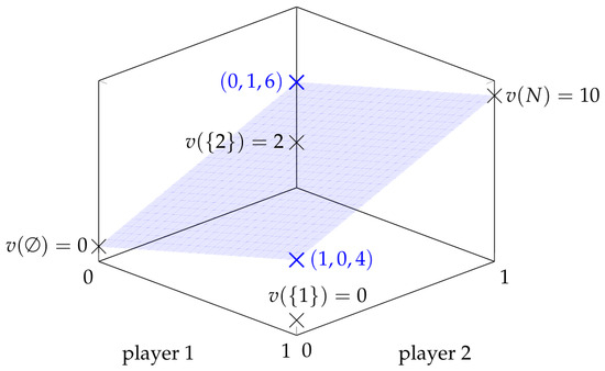
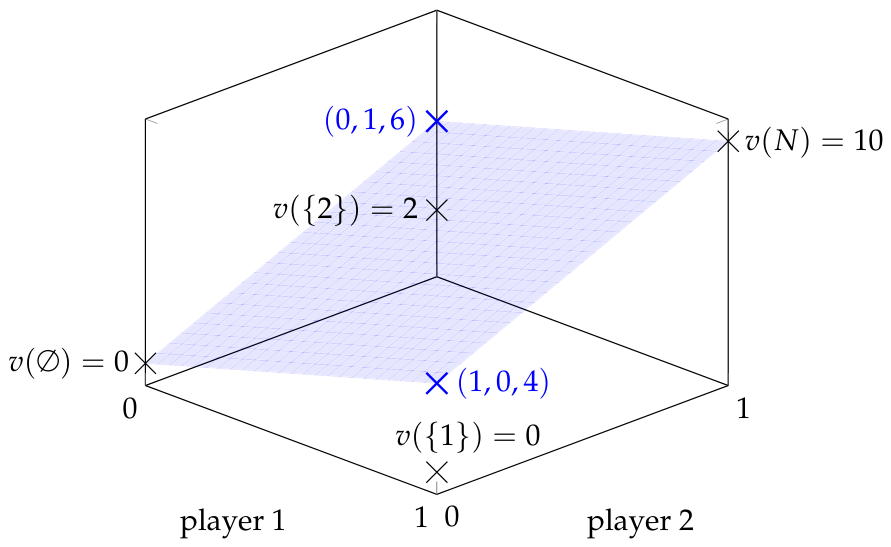
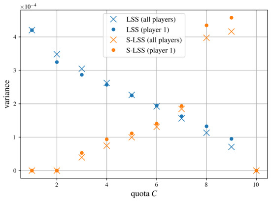
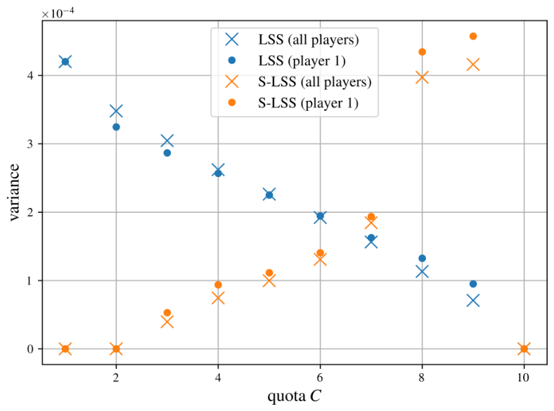
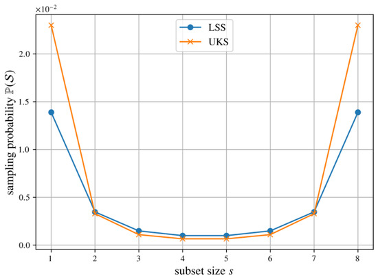
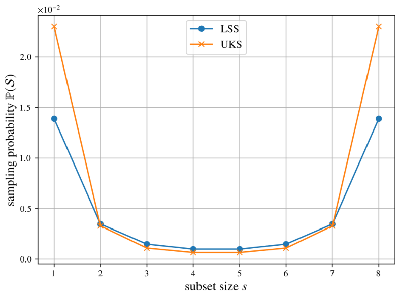
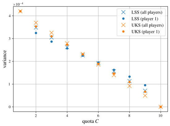
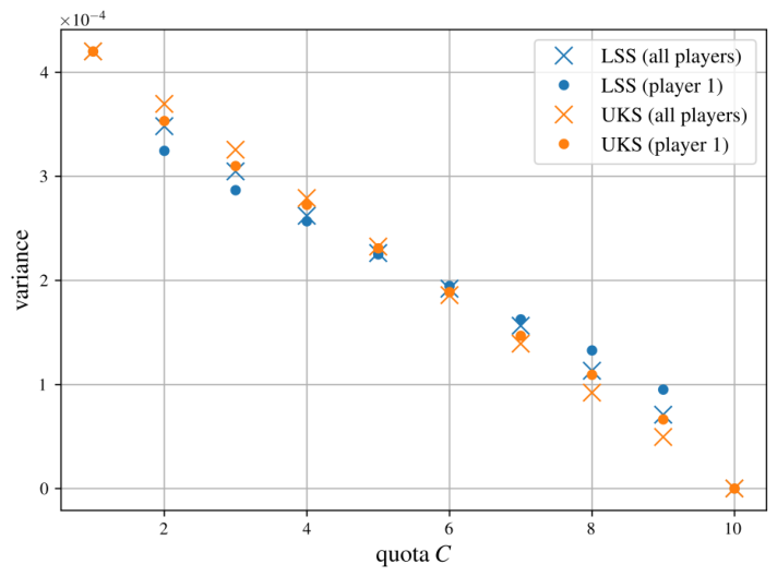
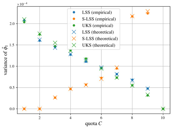
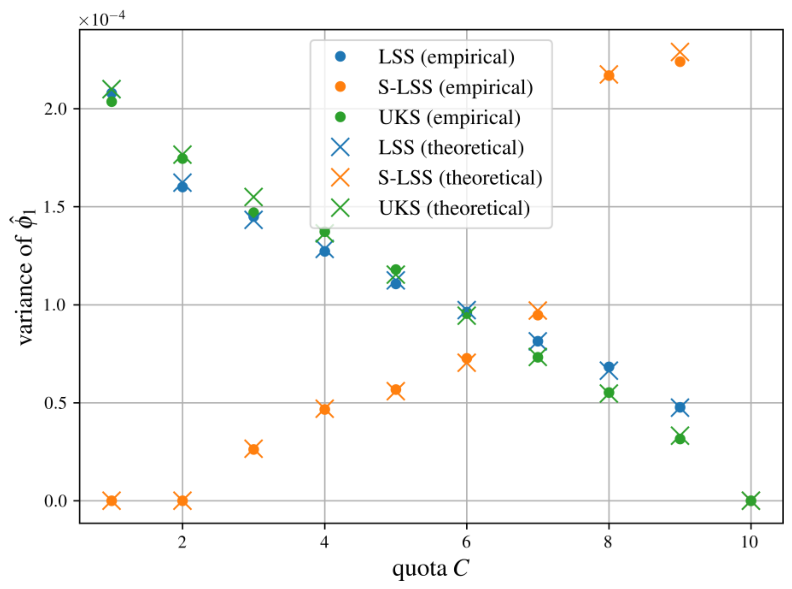
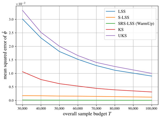
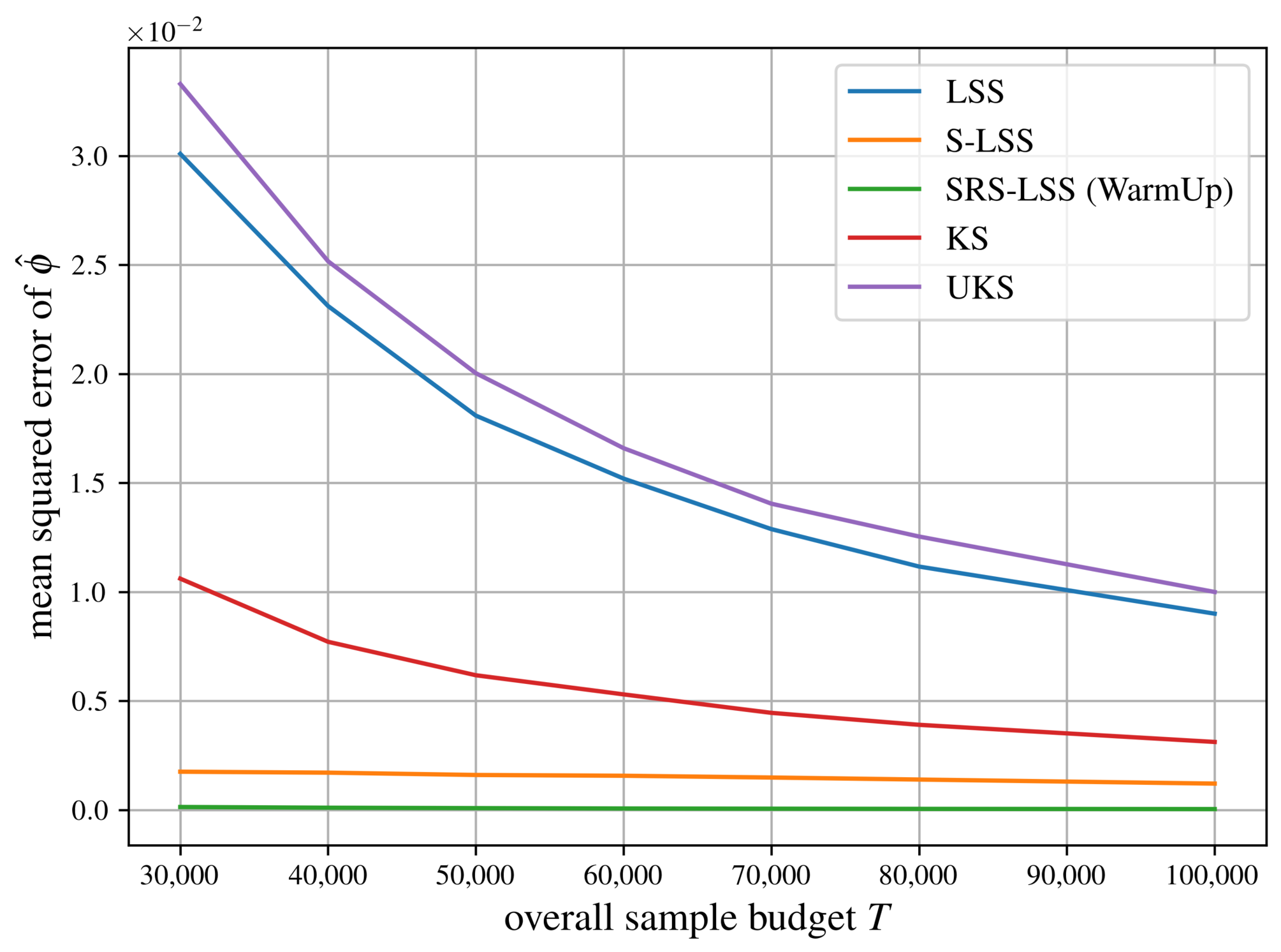
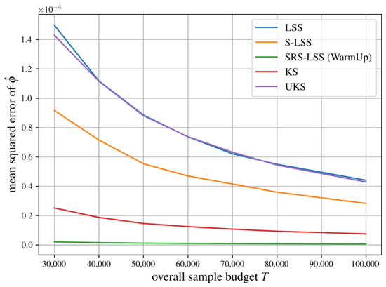
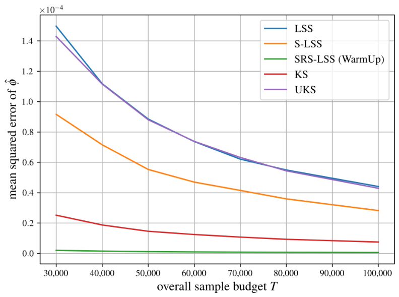
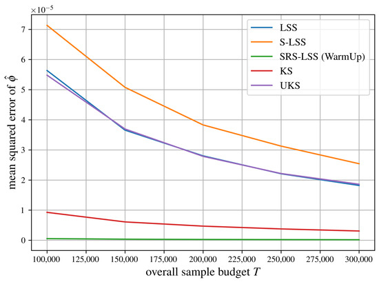
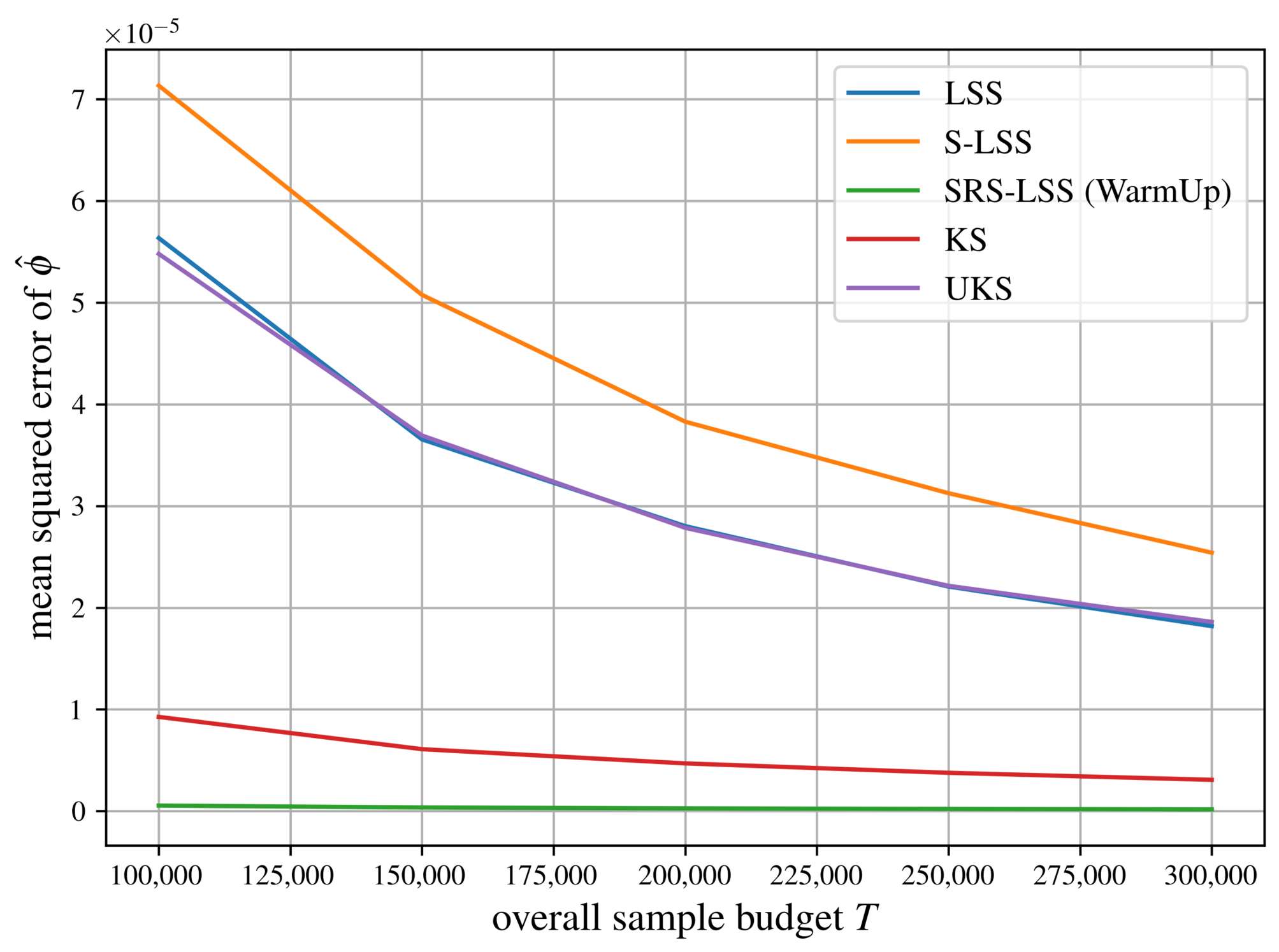
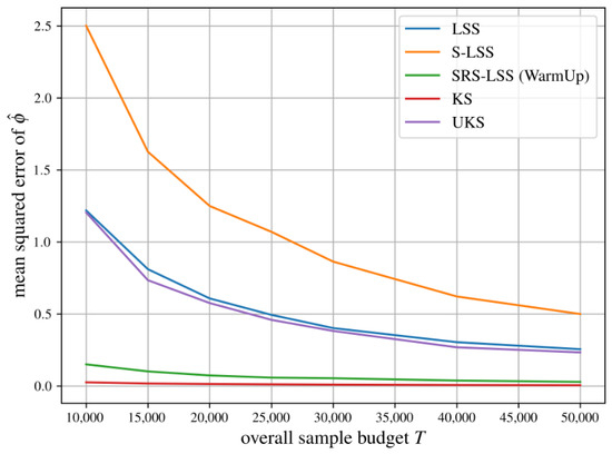
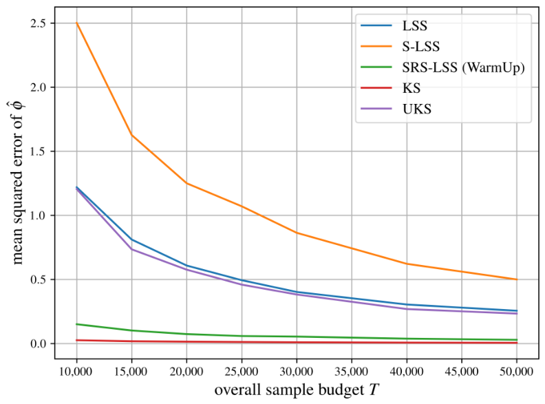
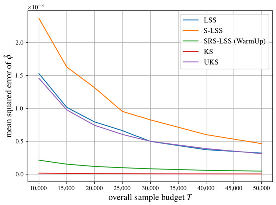
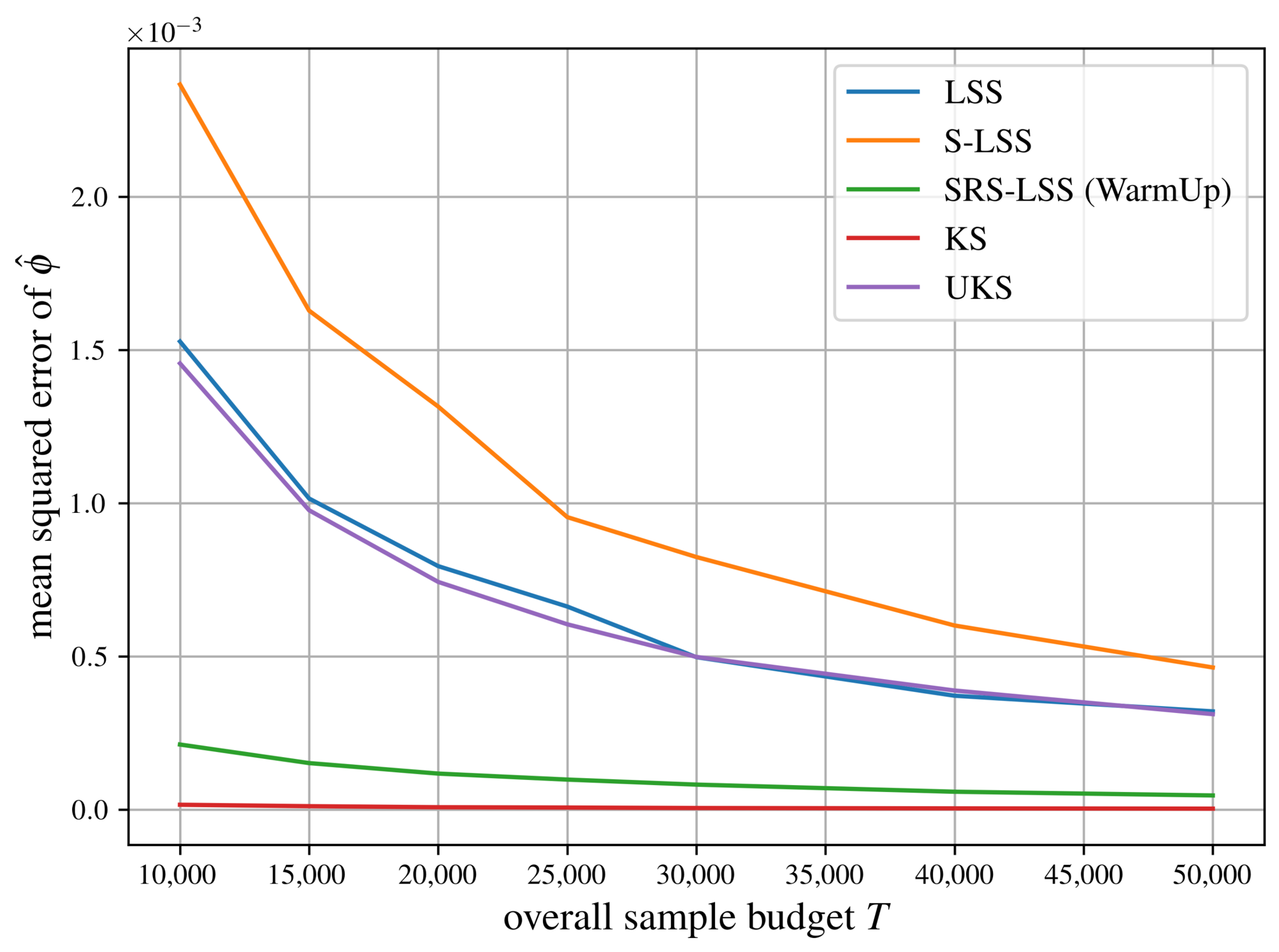
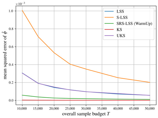
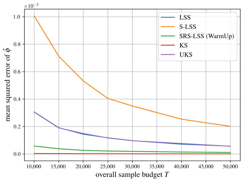

Disclaimer/Publisher’s Note: The statements, opinions and data contained in all publications are solely those of the individual author(s) and contributor(s) and not of MDPI and/or the editor(s). MDPI and/or the editor(s) disclaim responsibility for any injury to people or property resulting from any ideas, methods, instructions or products referred to in the content. |
© 2026 by the authors. Licensee MDPI, Basel, Switzerland. This article is an open access article distributed under the terms and conditions of the Creative Commons Attribution (CC BY) license.