Multidimensional Gap Decomposition for Diagnostic Prioritization in Biomass-Based Bioenergy Plants

Abstract

Biomass-based bioenergy plants are commonly compared using aggregate indices that locate a system on a utilization scale but conceal the dimensional structure of its remaining deficit. This study extends the Biopolygeneration Diagnostic Index (BDI) by defining the biopolygeneration gap as a weighted multidimensional distance between each plant profile and a synthetic componentwise best-demonstrated reference constructed exclusively from real operating plants. Each reference coordinate has been demonstrated independently; simultaneous feasibility of the complete vector is not assumed. The squared Euclidean metric is decomposed into criterion-level contributions to identify the dominant diagnostic leverage, without interpreting that leverage as a cost-optimal retrofit. The framework is evaluated using 34 literature-derived cases (21 real plants and 13 models) covering 11 conversion technologies and 16 countries. Relative gaps range from 0.198 to 0.827, and energy efficiency and exergetic output quality provide the dominant leverage in 31 of 34 baseline cases. Incremental information beyond the aggregate BDI is demonstrated by three real plants with nearly identical BDI values (0.606–0.629) but distinct dominant deficits: energy efficiency, exergetic quality, and coproduct valorization. Rank ordering remains stable under 90th-percentile and top-three-median references ($\rho =0.984$–$0.992$), alternative distance norms, local weight perturbations, and correction for the shared C1/C2 source. A bounded input-uncertainty scenario yields a mean rank correlation of 0.893 and shows that leverage stability is case-specific. The framework therefore supports transparent dimension-level diagnostic prioritization while preserving a clear boundary with techno-economic, environmental, and implementation decisions.

1. Introduction

Biomass is intrinsically multiproduct: the same resource can generate electricity, heat, fuels, and material coproducts with agronomic, energetic, or chemical functions [1,2]. This distinguishes biomass from renewable resources whose principal output is a single energy carrier and creates a multidimensional performance problem. A plant can be efficient in first-law terms while producing low-quality thermal outputs, depending heavily on imported auxiliary energy, dissipating recoverable heat, or discarding material streams. Consequently, a single conversion efficiency cannot represent integral biomass utilization [3,4].

Exergy analysis corrects the energetic equivalence between electricity and low-temperature heat and reveals inefficiencies hidden by energy balances [5,6,7]. Advanced exergy and 4E assessments add component-level causal and economic or environmental information [4,8,9]. Polygeneration and multi-energy-system studies represent multiple services and their technological integration [2,10]. Composite indices and multi-criteria methods, in turn, support comparison and selection using several criteria [11,12,13,14]. These approaches answer related but distinct questions: they quantify thermodynamic losses, describe system architecture, or rank alternatives; they do not necessarily quantify the multidimensional deficit of an operating plant relative to demonstrated sector performance and decompose that deficit by criterion.

The previously proposed Biopolygeneration Diagnostic Index (BDI) integrates five bounded dimensions: energy efficiency ($IE$), exergetic quality of outputs ($IQ$), thermal integration ($IT$), energy self-sufficiency ($IA$), and coproduct valorization ($IV$) [15]. The BDI is a standardized diagnostic decision function, not a conserved physical magnitude. Its five dimensions delimit a specific assessment domain: thermodynamic conversion and resource utilization. They are not claimed to constitute a complete sustainability index; capital cost, profitability, life-cycle impacts, emissions, reliability, feedstock logistics, and regulatory constraints require separate decision layers.

An aggregate index necessarily compresses the profile. Two plants can therefore obtain similar BDI values while their deficits occur in different dimensions. This is the methodological problem addressed here. Reference-point methods such as compromise programming and TOPSIS provide a formal language for distance to an ideal point [16,17], but their conventional use is ranking alternatives. The present study reorients that concept toward plant diagnosis: the distance is decomposed to determine which BDI dimension accounts for the largest share of the physical-performance deficit. This output is termed a dominant diagnostic leverage; it identifies the dimension where closing the demonstrated deficit would reduce the distance most, but it does not, without cost and feasibility information, prescribe a specific investment or implementation sequence.

The novelty is therefore not the invention of Euclidean distance itself. It lies in five linked elements: (i) embedding the complete BDI profile in a common five-dimensional performance space; (ii) constructing a reference exclusively from operating plants; (iii) using positive deficits so that modelled cases cannot generate negative gaps; (iv) exactly decomposing the squared distance into criterion contributions; and (v) testing whether the resulting ranking and leverage assignments survive changes in weights, frontier definition, distance norm, input uncertainty, technology family, and source dependence. The practical distinction from the aggregate BDI is demonstrated explicitly using plants with nearly identical BDI values but different dominant deficits.

Accordingly, this study aims to quantify and decompose the biopolygeneration gap of biomass bioenergy plants, evaluate the robustness of that diagnosis, and delimit its engineering interpretation. The framework is applied to 34 cases from peer-reviewed and authoritative technical literature: 21 real plants and 13 computational models, spanning 11 technologies and 16 countries. The analysis provides dimensional prioritization as a prerequisite for, rather than a substitute for, subsequent techno-economic and environmental decision-making.

2. Materials and Methods

2.1. Self-Contained Definition of the BDI Performance Profile

For plant i, the BDI profile is

$${\mathbf{p}}_i=(I{E}_i,I{Q}_i,I{T}_i,I{A}_i,I{V}_i),p_{i,k}\in [0,1].$$

(1)

The five sub-indices are reproduced here so that the present study can be read independently of the foundational paper [15]:

$$\begin{array}{cc}\hfill I{E}_i& ={\displaystyle \frac{E_{\mathrm{useful},i}}{E_{\mathrm{biomass},i}+E_{\mathrm{aux},i}^{\mathrm{ext}}}},\hfill \end{array}$$

(2)

$$\begin{array}{cc}\hfill I{Q}_i& ={\displaystyle \frac{{\sum }_{r}E{x}_{i,r}^{\mathrm{out}}}{{\sum }_r{E}_{i,r}^{\mathrm{out}}}},\hfill \end{array}$$

(3)

$$\begin{array}{cc}\hfill I{T}_i& ={\displaystyle \frac{Q_{\mathrm{recovered},i}}{Q_{\mathrm{available},i}}},\hfill \end{array}$$

(4)

$$\begin{array}{cc}\hfill I{A}_i& =1-{\displaystyle \frac{E_{\mathrm{aux},i}^{\mathrm{ext}}}{E_{\mathrm{aux},i}^{\mathrm{ext}}+E_{\mathrm{aux},i}^{\mathrm{int}}}},\hfill \end{array}$$

(5)

$$\begin{array}{cc}\hfill I{V}_i& ={\displaystyle \frac{{\sum }_{s}E{x}_{i,s}^{\mathrm{val}}}{{\sum }_{s}E{x}_{i,s}^{\mathrm{prod}}}}\hfill \end{array}$$

(6)

Here, $IE$ measures conversion of biomass and external auxiliary energy into useful outputs; $IQ$ measures thermodynamic quality of the output mix; $IT$ measures the fraction of available residual heat that is effectively reused; $IA$ measures independence from external auxiliary energy; and $IV$ measures the exergy fraction of generated coproducts incorporated into a defined value chain. The energy and exergy bases differ intentionally according to the physical object measured by each criterion.

The aggregate BDI is

$${\mathrm{BDI}}_i={\displaystyle \sum _{k=1}^5}{w}_k{p}_{i,k},\mathbf{w}=(0.40,0.24,0.14,0.14,0.08),\sum _k{w}_k=1.$$

(7)

The AHP consistency ratio reported in the foundational study indicates internal consistency of the pairwise judgments; it does not establish objective correctness or universal applicability of the weights. The vector is retained as the baseline preference structure for continuity, and its influence is tested using equal weights, local perturbations, and constrained and unrestricted weight simulations.

2.2. Assessment Boundary and Completeness of the Five Dimensions

The five dimensions are considered sufficient only for the stated diagnostic domain: thermodynamic performance, energy integration, operational energy autonomy, and utilization of secondary streams. They are not asserted to exhaust the environmental, economic, operational, logistical, social, or regulatory performance of a bioenergy project. Thus, the gap derived below is a thermodynamic and resource-utilization gap. A plant with a small gap may still be uneconomic, unreliable, environmentally burdensome, feedstock-constrained, or non-compliant. Conversely, those external constraints can prevent a technically identified deficit from being closed.

2.3. Synthetic Component-Wise Best-Demonstrated Reference

Let $\mathcal{R}$ denote the 21 real operating plants. The baseline reference is defined component-wise as

$$p_k^{*}=\underset{i\in \mathcal{R}}{max}{p}_{i,k},k=1,\dots ,5.$$

(8)

This vector is called the synthetic component-wise best-demonstrated reference. Each coordinate has been attained independently by at least one operating plant. The simultaneous technical, economic, and operational feasibility of the complete five-coordinate vector is neither assumed nor demonstrated. Accordingly, the reference is a diagnostic envelope analogous to the positive ideal solution of TOPSIS, not a claim that a single universally feasible plant design already exists.

Only real plants define the reference because unverified simulation optima could raise the benchmark without operational demonstration. Models are evaluated against the same reference but do not modify it. Robust alternatives are also tested: the 90th percentile of real-plant performance in each dimension and the median of the three highest real-plant values.

2.4. Biopolygeneration Gap and Alternative Distance Norms

For criterion k, the positive deficit is

$$d_{i,k}={(p_k^{*}-p_{i,k})}^{+}=max(0,p_k^{*}-p_{i,k}).$$

(9)

The general weighted $L_p$ gap is

$$\Delta B{P}_i^{\left(p\right)}={\left({\displaystyle \sum _{k=1}^5}{w}_k{d}_{i,k}^p\right)}^{1/p},p\ge 1.$$

(10)

The baseline metric is the weighted Euclidean distance

$$\Delta B{P}_i=\sqrt{{\displaystyle \sum _{k=1}^5}{w}_k{d}_{i,k}^2}.$$

(11)

Its quadratic form penalizes concentrated deficits and permits exact additive decomposition. Robustness is examined against $L_1$ and $L_{\infty }$ norms applied to the consistently scaled coordinates $z_{i,k}=\sqrt{w_k}{d}_{i,k}$:

$$L_{1,i}=\sum _k{z}_{i,k},L_{\infty ,i}=\underset{k}{max}{z}_{i,k}.$$

(12)

The relative gap is normalized using the real-plant anti-reference $p_k^{-}={min}_{i\in \mathcal{R}}{p}_{i,k}$:

$${\delta }_i={\displaystyle \frac{\Delta B{P}_i}{\Delta B{P}_{max}}},\Delta B{P}_{max}=\sqrt{\sum _{k=1}^5{w}_k{(p_k^{*}-p_k^{-})}^2}.$$

(13)

2.5. Dimensional Decomposition and Dominant Diagnostic Leverage

For $\Delta B{P}_i>0$, the contribution of criterion k is

$${\gamma }_{i,k}={\displaystyle \frac{w_k{d}_{i,k}^2}{\Delta B{P}_i^2}},\sum _k{\gamma }_{i,k}=1.$$

(14)

The dominant diagnostic leverage is

$${\mathcal{l}}_i=arg\underset{k}{max}{\gamma }_{i,k}.$$

(15)

It identifies the dimension whose complete closure to the reference would produce the greatest reduction in squared distance. It does not identify the least-cost intervention, guarantee technical transferability, or replace detailed component-level design.

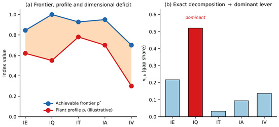
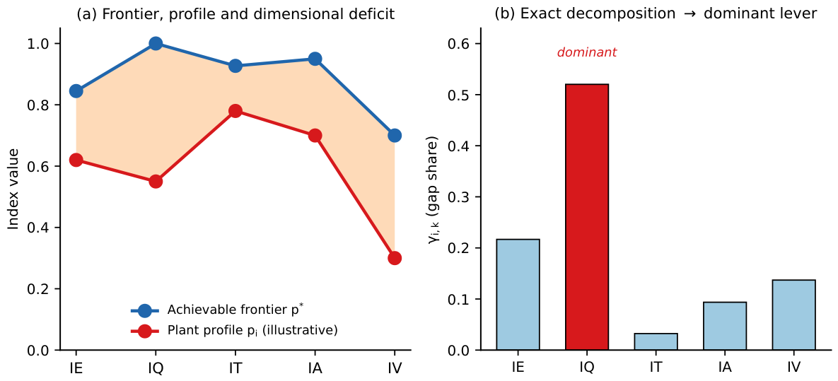
Figure 1 summarizes the complete diagnostic construction.

Figure 1. Schematic of the framework. (a) The weighted positive deficits between a plant profile and the best-demonstrated reference define the biopolygeneration gap; (b) the squared metric is decomposed exactly into dimensional contributions ${\gamma }_{i,k}$, whose maximum identifies the dominant diagnostic leverage (here $IQ$). The profile is illustrative and corresponds to no dataset case.

Figure 1a shows how the positive dimensional deficits generate the distance to the reference, and Figure 1b shows the exact decomposition that isolates the dimension carrying the largest share of that distance.

2.6. Conventional Severity Bands

For descriptive interpretation, $\delta <0.20$ is labelled close to the reference, $0.20\le \delta <0.50$ moderate, $0.50\le \delta <0.80$ severe, and $\delta \ge 0.80$ critical. These thresholds are conventions rather than physical failure limits and are interpreted only within the present dataset and normalization.

2.7. Case Identification, Data Provenance, and Traceability

The case set was assembled through a structured literature-based identification process rather than a population-representative systematic review. Cases were eligible when the source supplied sufficient energy, exergy, heat-recovery, auxiliary-energy, and coproduct information to calculate or transparently reconstruct all five sub-indices. Cases were excluded when the source could not be verified, the system boundary was incompatible, or the information was insufficient for a reproducible profile. This data-completeness criterion necessarily creates selection bias toward well-documented plants and models; therefore, the sample is treated as an analytical case set and not as a random representation of the global biomass sector.

The resulting matrix contains 34 cases, 21 real plants and 13 models, across 11 conversion technologies and 16 countries. The Supplementary Materials provide the exact $34\times 5$ sub-index matrix, the BDI and gap calculations, source DOI, technology, country, real/model classification, bibliographic audit, and data-provenance status. These materials reproduce every analysis reported here from the harmonized matrix. Where an original source does not expose complete intermediate balances or measurement covariance, the provenance register flags that limitation rather than inferring unreported precision.

Legacy identifiers are retained to preserve traceability to the audited dataset. C19 was excluded because its source failed the predefined reliability criteria, and subsequent cases were not renumbered; therefore, 34 valid cases include the identifier C35. The C25 record was replaced before analysis because its original DOI could not be verified; the replacement met the same data-completeness and system-boundary criteria, and all five sub-indices were recalculated. C1 and C2 represent two operating configurations reported in the same publication and are handled explicitly in the source-level dependence analysis.

2.8. Robustness and Uncertainty Analyses

• Weights.

Each baseline weight is perturbed by $\pm 20\%$ and $\pm 30\%$ followed by renormalization. Equal weights provide a non-AHP comparison. Two Monte Carlo analyses ($N=10,000$) are performed over the weight simplex: a constrained Dirichlet sample preserving the qualitative hierarchy ($w_{IE}$ maximal and $w_{IV}$ minimal), and an unrestricted Dirichlet stress test. The latter tests how strongly conclusions depend on the adopted normative structure and is not expected to reproduce the baseline hierarchy.

• Reference definition.

The component-wise maximum reference is compared with a componentwise 90th-percentile reference and a componentwise median-of-top-three reference. A leave-one-reference-plant-out analysis is also retained. Rank stability is quantified by Spearman correlation and dominant-leverage agreement.

• Distance norm.

Rankings from $L_1$ and $L_{\infty }$ are compared with the baseline $L_2$ ordering using Spearman and Kendall correlations.

• Technology-family references.

Exploratory references are constructed for technology families containing operational plants: anaerobic digestion/biogas, gasification, and combustion/CHP. Pyrolysis/biorefinery cases are not assigned a real-plant family frontier because the available cases in that family are models. These analyses distinguish sector-wide benchmarking from within-family benchmarking.

• Input uncertainty scenario.

Because most source papers do not report harmonized measurement covariance, formal metrological uncertainty cannot be reconstructed retrospectively. Instead, an epistemic scenario consistent with the foundational BDI sensitivity analysis is applied. Conditional on the baseline matrix, sub-indices are perturbed independently using truncated-normal distributions bounded in $[0,1]$, with relative standard deviations of 10% for $IE$, $IQ$, and $IT$, and 20% for $IA$ and $IV$. The component-wise real-plant reference and anti-reference are recalculated in every one of the $N=10,000$ realizations (random seed 20260712). Reported intervals are scenario intervals, not experimental confidence intervals.

• Dependence and covariance.

The real-versus-model comparison is repeated after replacing C1 and C2 by the arithmetic mean of their relative gaps, yielding one source-level observation. Pearson and Spearman sub-index correlations, variance inflation factors (VIF), and condition numbers are examined. For covariance sensitivity, the positive-deficit vector ${\mathbf{d}}_i={(\mathbf{p}*-{\mathbf{p}}_i)}^{+}$ is evaluated using

$$D_{M,i}=\sqrt{{\mathbf{d}}_i^{\mathsf{T}}{\mathbf{S}}^{-1}{\mathbf{d}}_i},$$

(16)

where $\mathbf{S}$ is the covariance matrix of the five sub-indices. Results are reported for covariance estimated from all 34 cases and, as a secondary check, from the 21 real plants. Mahalanobis distance is not adopted as the primary metric because it is sample-dependent, changes the normative role of the AHP weights, and does not preserve the non-negative additive criterion decomposition required for diagnostic leverage.

2.9. Statistical Analysis

Descriptive statistics are reported for the complete set and for real plants and models. Real/model differences are evaluated with a two-sided Mann–Whitney test, Cliff’s delta, and a 10,000-resample percentile bootstrap interval for the median difference. Association between BDI and $\delta$ is assessed by Spearman and Pearson correlations. These tests characterize the literature case set; they do not support population-wide prevalence claims. Analyses were implemented in Python using SciPy at $\alpha =0.05$.

2.10. Quantified C9 Diagnostic Scenarios

To demonstrate how the decomposition can support, but not replace, engineering scenario analysis, two C9 counterfactuals are evaluated. In the first, only $IE$ is raised to the real-plant $IE$ reference while all other dimensions remain fixed; this is a mathematical upper-bound test of the dominant deficit. In the second, the dimensional change observed between the paired C1 configuration without CHP and C2 with CHP is transferred to C9 and bounded to $[0,1]$. This technology-analogue scenario is explicitly conditional on transferability and is not interpreted as a causal forecast or economic recommendation.

3. Results

3.1. Baseline Reference and Gap Distribution

The 21 real plants define the synthetic component-wise best-demonstrated reference

$$\mathbf{p}*=(0.845,1.000,0.927,0.950,0.700),$$

(17)

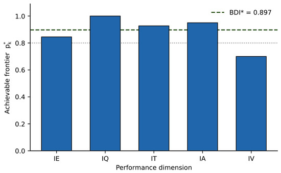
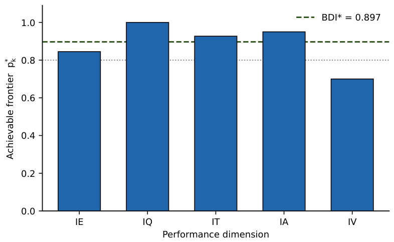
with ${\mathrm{BDI}}^{*}=0.897$. The coordinates are supplied by different operating plants; no individual case attains the complete vector. The real-plant anti-reference is $(0.200,0.296,0,0.450,0.050)$ and $\Delta B{P}_{max}=0.6888$. The dimensional structure of this reference is shown in Figure 2.

Figure 2. Best-demonstrated reference $p^{*}$ by dimension, with the aggregate line $BD{I}^{*}=0.897$. Coproduct valorization ($IV$) is the only coordinate below 0.80.

Exergetic quality reaches unity, supplied by an electricity-led plant, whereas coproduct valorization is the only coordinate that stays below 0.80, indicating that valorization is the least mature dimension of the sampled sector rather than the deficit of a single case.

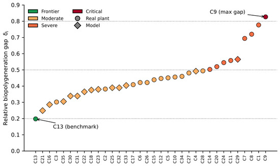
Across the 34 cases, $\delta$ ranges from 0.198 for C13 to 0.827 for C9, with median 0.431. One case is close to the reference, 24 are moderate, eight severe, and one critical. Figure 3 orders the complete distribution, and Table 1 reports the full per-case diagnosis.

Figure 3. Relative biopolygeneration gap ${\delta }_i$ for the 34 cases, ordered from lowest to highest. Circle = real plant; diamond = model. Severity bands are conventional and dataset-dependent.

Table 1. Gap diagnosis of the 34 cases, ordered by ascending ${\delta }_i$. Each case is referenced to its original source. Type: R = real plant, M = model.

ID	Technology	Country	Type	BDI	$\mathbf{\Delta }{\mathbf{BP}}_{\mathit{i}}$	${\mathit{\delta }}_{\mathit{i}}$	${\mathcal{l}}_{\mathit{i}}$
C13	Bagasse cogeneration 33 MW [18]	Brazil	R	0.773	0.136	0.198	IQ
C21	Solar pyrolysis + biochar [19]	Spain	M	0.751	0.172	0.249	IE
C16	Bagasse gasif. CFB + CC [20]	Brazil	M	0.705	0.197	0.286	IE
C3	ORC+GAX microturbine (trigen.) [21]	Cyprus	R	0.733	0.208	0.302	IQ
C35	Palm-sugar biorefinery [22]	Brazil	M	0.710	0.210	0.305	IQ
C30	Biomass + Stirling + sCO2 [23]	Iran	M	0.687	0.234	0.339	IQ
C31	Biomass-coal cofiring CCCHP [24]	China	M	0.684	0.234	0.339	IQ
C22	Multi-feedstock pyrolysis (TEA) [25]	USA	M	0.675	0.252	0.365	IE
C18	EFGT + SRC + ORC + ARC cogeneration [26]	Iran	M	0.675	0.259	0.376	IQ
C23	Flax straw pyrolysis [27]	Canada	M	0.659	0.262	0.380	IA
C2	Biogas ICE with CHP [28]	China	R	0.715	0.263	0.382	IQ
C25	MSW gasif. + SOFC/GT/ORC + AHP [29]	China	M	0.687	0.268	0.390	IE
C32	Pellets exergoeconomic CHP [30]	Finland	M	0.656	0.269	0.390	IQ
C33	Microalgae gasif. + H2 [31]	Saudi Arabia	M	0.655	0.278	0.404	IE
C17	Gasification + SOFC + CCHP [32]	China	R	0.664	0.282	0.409	IQ
C6	Landfill gas CHP [33]	Poland	R	0.629	0.291	0.422	IV
C26	Wood chips CHP district heating [34]	Sweden	R	0.705	0.291	0.422	IQ
C15	Biomass oxy-fuel gasif. CFB [35]	China	R	0.606	0.302	0.439	IE
C12	Bagasse cogeneration + ethanol [36]	Brazil	R	0.676	0.308	0.447	IQ
C5	Agricultural biogas 1 MWe CHP [37]	Poland	R	0.600	0.311	0.451	IQ
C10	POME biogas CHP [38]	Indonesia	R	0.609	0.314	0.456	IQ
C34	Charcoal Rankine CHP [39]	Brazil	R	0.586	0.317	0.460	IE
C27	Cattle manure CHP biogas [40]	Poland	R	0.580	0.331	0.481	IE
C4	DFB wood gasif. + DH [41]	France	M	0.637	0.339	0.492	IQ
C28	Co-digestion cattle + swine [42]	Brazil	R	0.577	0.341	0.494	IE
C14	Rice husk gasif. + CCS [43]	India	R	0.571	0.347	0.503	IQ
C20	AcoD sludge + coffee [44]	Poland	R	0.568	0.358	0.520	IQ
C24	MSW incineration oxy + PtG [45]	Italy	R	0.541	0.375	0.545	IE
C11	Biogas trigeneration (CCHP) [46]	Turkey	R	0.619	0.384	0.558	IQ
C29	Microalgae biodiesel [47]	Brazil	M	0.557	0.389	0.565	IE
C7	AD-CHP WWTP (sludge) [48]	Iran	R	0.436	0.478	0.694	IE
C8	AD + biofertilizer (OFMSW) [49]	Iran	R	0.513	0.496	0.720	IT
C1	Biogas ICE without CHP [28]	China	R	0.453	0.535	0.777	IE
C9	POME biogas ICE [50]	Indonesia	R	0.426	0.569	0.827	IE

The ordered profile in Figure 3 rises smoothly from C13 to C9 without discontinuities, and real plants and models are interleaved across the moderate band rather than forming separate clusters, indicating that the gap varies continuously with plant configuration rather than with the real-or-model distinction alone.

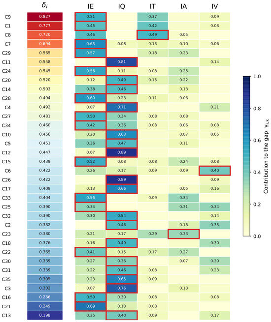
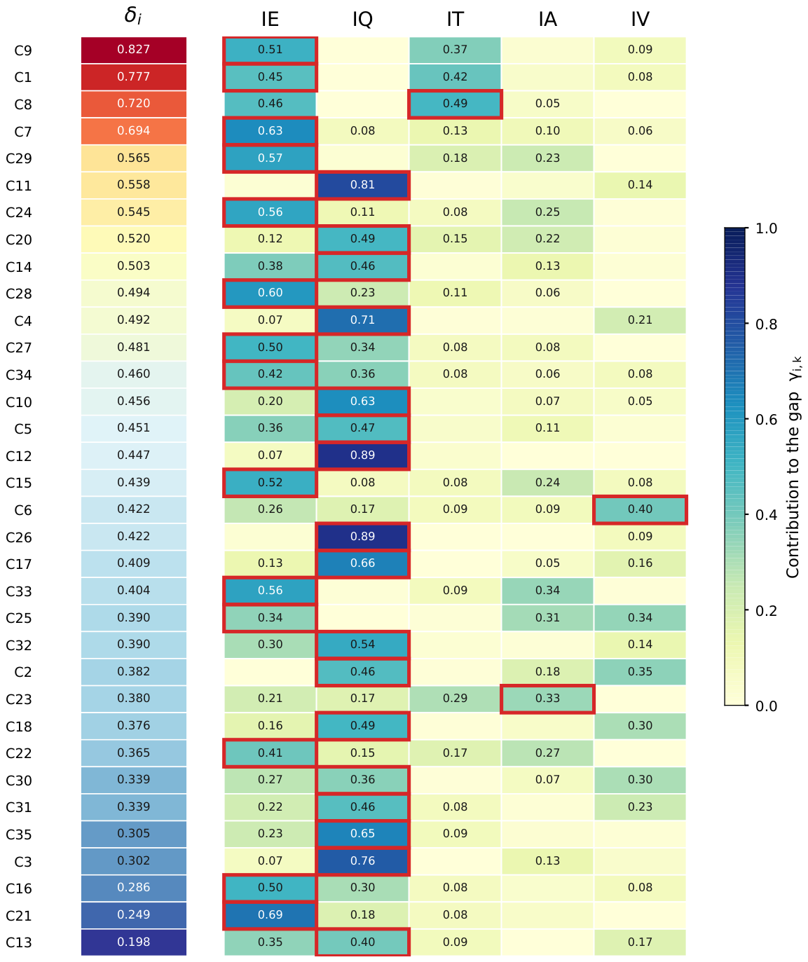
Table 1 makes the coexistence of aggregate similarity and dimensional divergence explicit: several cases with comparable BDI values are separated by their relative gap and, more importantly, carry different dominant leverages ${\mathcal{l}}_i$, which is the information the following decomposition isolates. The last column already anticipates that $IE$ and $IQ$ recur as the prevailing leverages, while $IT$, $IA$, and $IV$ appear only in isolated cases.

3.2. Dimensional Decomposition

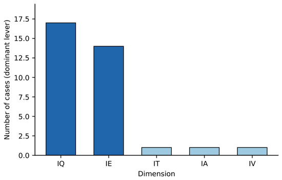
Exergetic quality ($IQ$) is the dominant diagnostic leverage in 17 cases and energy efficiency ($IE$) in 14; together they account for 31 of 34 cases. $IT$, $IA$, and $IV$ dominate one case each. This distribution results jointly from the observed deficits and the baseline weight vector; it is not interpreted as a universal sector prevalence. The aggregate frequency of dominant levers is shown in Figure 4.

Figure 4. Frequency of the dominant diagnostic leverage across the 34 cases. Exergetic quality ($IQ$) and energy efficiency ($IE$) account for 31 of the 34 cases.

The two prevailing levers arise from structural properties of the reference and the weight vector: $IQ$ because its ceiling is fixed at the exergy limit, and $IE$ because it carries the largest weight; the remaining dimensions dominate isolated cases only. The complete case-by-case decomposition is mapped in Figure 5.

Figure 5. Exact decomposition of the squared baseline gap into dimensional contributions ${\gamma }_{i,k}$. The highlighted cell identifies the dominant diagnostic leverage; near-ties should be interpreted as ambiguous rather than unequivocal.

The high-gap tail is mainly $IE$-dominated, reflecting limited basic energy recovery. Many moderate cases are $IQ$-dominated because useful thermal outputs increase first-law utilization while retaining lower exergy quality than electricity or fuels. This lower exergetic quality should not be read as a general weakness of heat-led systems: the value of heat depends on its temperature, on the presence of a matched thermal demand, and on the fuel it displaces. $IQ$ measures the thermodynamic quality of the output mix, not the economic or end-use value of the delivered service; accordingly, a low $IQ$ signals a diagnostic priority to examine, not evidence that a heat-led configuration is inferior, and raising exergetic output is therefore reported as one candidate pathway rather than the recommended one. C13 is a clear ambiguity case: its $IE$ and $IQ$ contributions are close, and the input-uncertainty analysis confirms that a single deterministic label is not robust for this case.

3.3. Direct Evidence of Information Beyond the Aggregate BDI

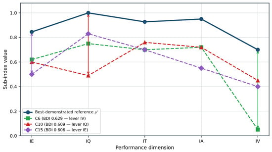
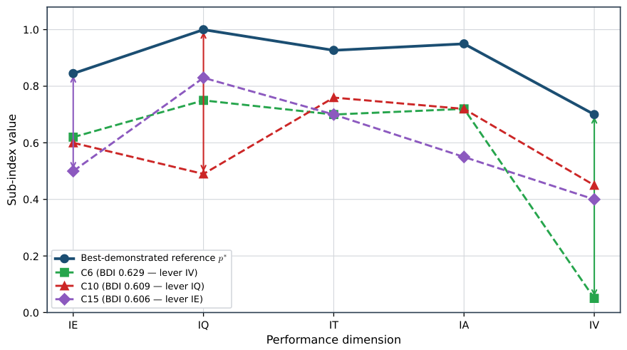
The strongest demonstration of incremental information is not the contrast between the best and worst plants, which any aggregate score separates, but the comparison of plants with nearly identical BDI values. C6, C10, and C15 have BDI values of 0.629, 0.609, and 0.606, respectively, a spread of only 0.023. Nevertheless, their dominant deficits occur in three distinct dimensions: coproduct valorization ($IV$) for C6, exergetic quality ($IQ$) for C10, and energy efficiency ($IE$) for C15. Their dominant contribution shares are 0.399, 0.630, and 0.521, respectively. These three profiles are compared dimension by dimension in Figure 6.

Figure 6. Three plants with similar aggregate BDI values but different dimensional profiles and dominant diagnostic leverage. The example demonstrates the information gained by retaining and decomposing the multidimensional profile.

Figure 6 shows that the three profiles cross rather than run parallel: C6 tracks the reference closely on $IE$ and $IQ$ but collapses on $IV$; C10 is limited chiefly by exergetic quality; and C15 falls furthest on energy efficiency. A single aggregate value therefore maps to three distinct engineering situations, each pointing to a different follow-up analysis.

3.4. Reference and Distance Robustness

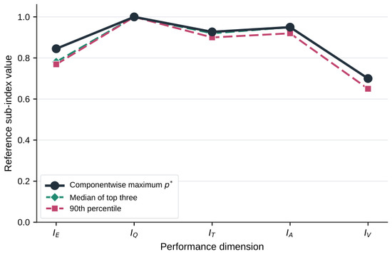
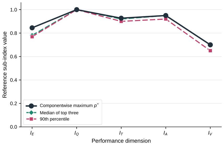
The 90th-percentile reference is $(0.769,1.000,0.900,0.920,0.650)$ and the median-of-top-three reference is $(0.781,1.000,0.920,0.950,0.700)$. Their gap rankings correlate with the maximum-based ordering at $\rho =0.984$ and $\rho =0.992$, respectively; C13 and C9 remain the minimum- and maximum-gap cases. With the normalization denominator recalculated for each alternative reference, two cases change severity under the 90th-percentile definition and one under the median-of-top-three definition. The P90 lever agrees with the baseline in 28 of 34 cases (82.4%), and the median-of-top-three lever likewise agrees in 28 of 34; independently, $IE$ and $IQ$ are the dominant lever in 28 of 34 cases under the P90 reference. Thus, rank ordering is highly stable, whereas some criterion assignments and threshold-based labels near decision boundaries depend on the reference definition. Figure 7 compares the three reference vectors by dimension.

Figure 7. Baseline and robust component-wise reference vectors. Each remains a synthetic diagnostic envelope; robust definitions reduce dependence on a single maximum observation.

Figure 7 shows that the three reference vectors coincide on $IQ$ at the exergy ceiling and differ mainly on $IE$ and $IV$, where the percentile and median-of-top-three definitions sit slightly below the component-wise maximum. This visual proximity is the geometric reason the rankings remain almost unchanged while a few boundary labels shift, confirming that the diagnosis does not hinge on a single extreme observation.

Using the same $\sqrt{w_k}$-scaled deficits, $L_1$ and $L_{\infty }$ both preserve the extreme cases. Relative to $L_2$, Spearman correlations are 0.927 for both alternatives; Kendall correlations are 0.797 and 0.779, respectively. Thus, the principal diagnostic structure is not created by the Euclidean norm, although mid-ranking positions are norm-sensitive.

3.5. Weight and Input-Uncertainty Sensitivity

Local perturbations of $\pm 20\%$ and $\pm 30\%$ preserve the baseline ordering with $\rho \ge 0.981$. Equal weighting gives $\rho =0.877$ and preserves C13 and C9 as the extremes, but only 52.9% of dominant-leverage labels agree with the AHP baseline. This confirms that rank extremes are robust while criterion-level prioritization appropriately remains sensitive to the normative meaning of weights.

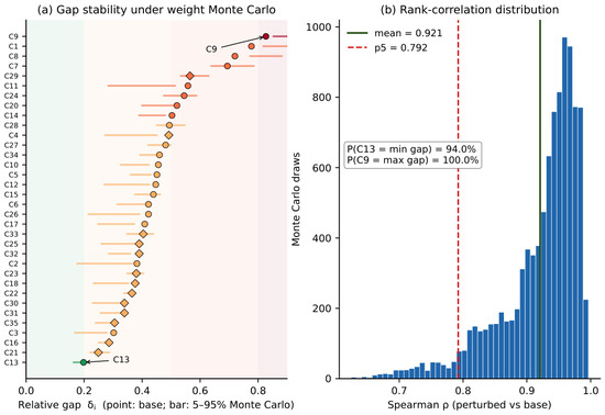
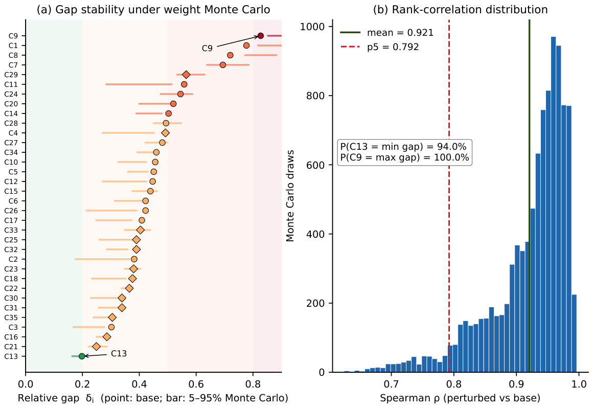
Under the constrained Dirichlet simulation, mean rank correlation is 0.904 (5th percentile 0.737); C13 and C9 retain the extreme ranks in 95.4% and 98.8% of realizations. Under the unrestricted Dirichlet stress test, mean correlation falls to 0.733 (5th percentile 0.444), with extreme-rank probabilities of 45.6% and 76.4%. The unrestricted result is important: the AHP vector is not universal, and abandoning its hierarchy can materially alter the diagnosis. Figure 8 summarizes the constrained weight simulation.

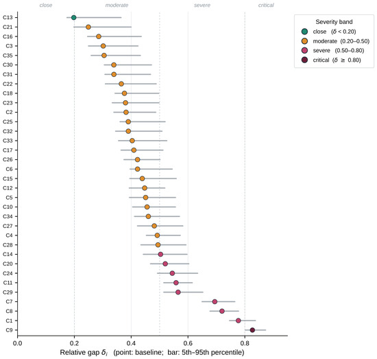
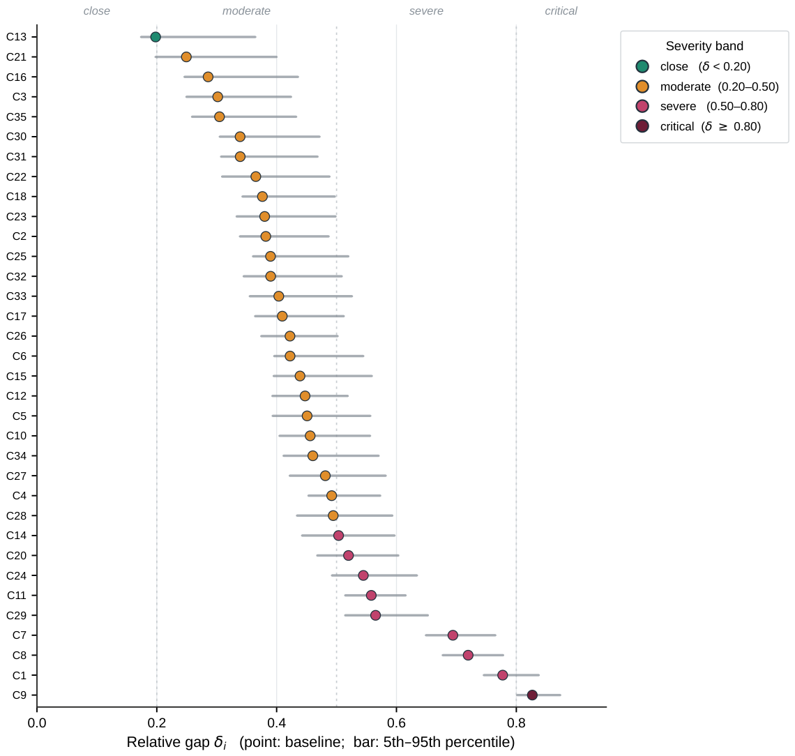
Figure 8. Robustness of the gap ordering under weight uncertainty (constrained simplex, $w_{IE}$ maximal and $w_{IV}$ minimal). (a) Per-case relative gap (point: baseline; bar: 5–95% Monte Carlo interval). (b) Distribution of Spearman rank correlation between each perturbed ordering and the baseline.

Figure 8a shows that the extreme cases retain narrow intervals while mid-ranking cases are more weight-sensitive, and Figure 8b shows the rank-correlation distribution centred at 0.904, confirming that the overall ordering is preserved under admissible weightings.

The input-uncertainty scenario yields a mean rank correlation of 0.893 (5th percentile 0.827) and mean dominant-leverage agreement of 71.1%. C9 remains the maximum-gap case in 95.4% of realizations and retains $IE$ as its dominant leverage in 97.5%. Lever stability is 80.1% for C6, 87.9% for C10, and 91.5% for C15, supporting the similar-BDI counterexample. By contrast, C13 retains $IQ$ as the deterministic leverage in only 15.6% of realizations, confirming that it should be reported as an $IE$–$IQ$ ambiguity rather than as an unequivocal priority. The baseline gaps and their scenario intervals are shown in Figure 9.

Figure 9. Baseline relative gaps and 5th–95th percentile intervals under the bounded input-uncertainty scenario. Intervals represent epistemic scenario variation, not measurement confidence intervals.

Figure 9 shows that the scenario intervals overlap between neighbouring mid-ranking cases but not at the extremes: the intervals for C13 and C9 remain clearly separated from the rest, which is the graphical counterpart of their high extreme-rank probabilities. The width of the intervals also scales with the baseline gap, so the least favourable plants carry the largest absolute uncertainty without changing their position in the ordering.

3.6. Global Versus Technology-Family References

For anaerobic digestion/biogas, the family-specific and global rankings are almost identical ($\rho =0.995$) and all dominant-leverage labels agree. For gasification, $\rho =0.952$ with 62.5% leverage agreement; for combustion/CHP, $\rho =0.976$ with 62.5% agreement. The global reference is therefore suitable for sector-wide comparison, but family references can alter the criterion selected for follow-up engineering analysis. No real-plant pyrolysis/biorefinery reference is reported because all available cases in that family are models.

3.7. Real Plants, Models, Source Dependence, and Covariance Structure

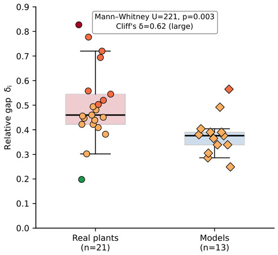
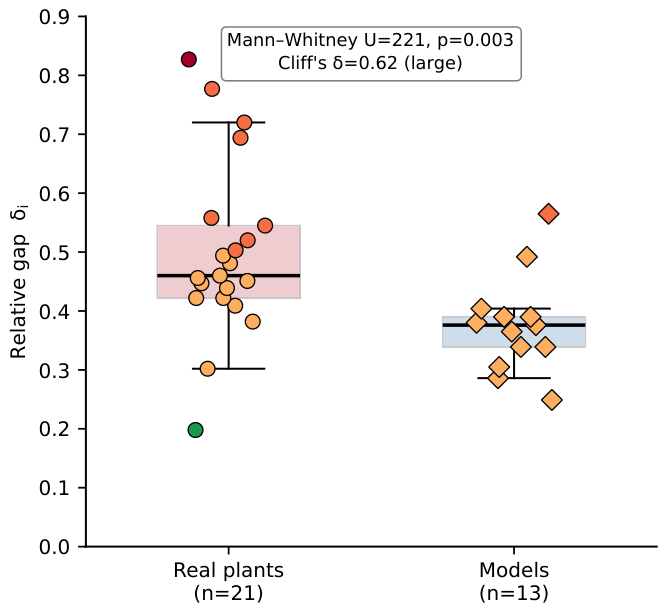
Real plants have a median $\delta$ of 0.460 versus 0.376 for models. The case-level Mann–Whitney test gives $U=221$, $p=0.0029$, and Cliff’s $\delta =0.619$. After collapsing the dependent C1/C2 pair into one source-level observation, the contrast remains: $U=213$, $p=0.0024$, and Cliff’s $\delta =0.638$. Thus, the result is not driven by treating the paired configurations as independent publications. It remains a case-set result and is not generalized to all operating plants and models. Figure 10 shows the two distributions.

Figure 10. Distribution of the relative gap ${\delta }_i$ for real plants ($n=21$) and models ($n=13$); points coloured by severity. The Mann–Whitney statistic, p-value, and Cliff’s $\delta$ are indicated.

Models concentrate in the moderate band and below the real-plant median, giving a visual counterpart to the significant contrast and supporting the exclusion of models from the reference set.

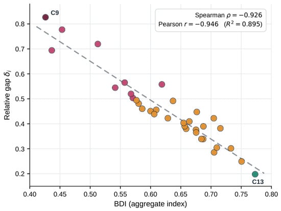
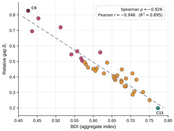
BDI and relative gap are strongly but imperfectly associated: Spearman $\rho =-0.926$ and Pearson $r=-0.946$ ($R^2=0.895$). The similar-BDI example in Figure 6 shows why a high correlation does not make the decomposition redundant. The overall association is shown in Figure 11.

Figure 11. Relationship between BDI and the relative gap ${\delta }_i$ across the 34 cases, with Spearman and Pearson coefficients; points coloured by severity.

The tight but imperfect trend confirms internal coherence, whereas the vertical spread of cases at nearly identical BDI is precisely the residual information that the dimensional decomposition recovers.

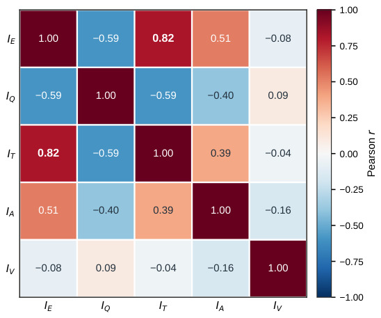
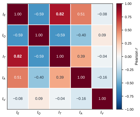
Across all 34 cases, the largest Pearson sub-index correlation is 0.817 between $IE$ and $IT$. VIF values are 3.58 ($IE$), 1.65 ($IQ$), 3.21 ($IT$), 1.42 ($IA$), and 1.03 ($IV$), with a correlation-matrix condition number of 15.9. These values indicate moderate dependence, especially between conversion efficiency and heat integration, but not singularity. Using the full-case covariance matrix in Equation (16), the Mahalanobis ordering correlates with the baseline at $\rho =0.924$; C13 remains the minimum-distance case, whereas C7 replaces C9 at the maximum. Using covariance estimated only from the 21 real plants reduces concordance to $\rho =0.844$ and changes both extremes. This estimator sensitivity is a substantive limitation: the Euclidean ranking is not covariance-invariant. Mahalanobis distance is therefore reported as a stress test rather than a replacement for the weighted, additively decomposable diagnostic metric. The full correlation structure of the five sub-indices is shown in Figure 12.

Figure 12. Pearson correlation matrix of the five sub-indices across the 34 cases. Only the $IE$–$IT$ pair exceeds 0.8.

Only the energy-efficiency—thermal-integration pair shows strong correlation ($r=0.82$); all other pairs are weak to moderate, consistent with the low-to-moderate variance inflation factors and confirming that the five dimensions are not redundant.

3.8. Quantified C9 Scenarios

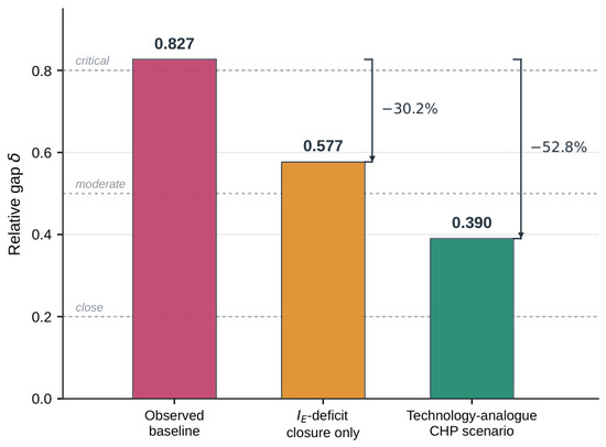
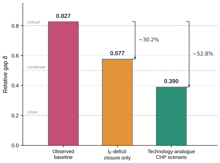
C9 has $\mathrm{BDI}=0.426$, $\Delta BP=0.569$, and $\delta =0.827$, with $IE$ as the dominant leverage. Raising only $IE$ from 0.200 to the global real-plant reference of 0.845, while leaving the other dimensions unchanged, gives $\mathrm{BDI}=0.684$ and $\delta =0.577$: a 30.2% gap reduction and a change from critical to severe. This is the exact maximum reduction obtainable by closing only the identified $IE$ deficit within the metric.

Applying the C1-to-C2 CHP profile change to C9 gives the conditional profile $(0.769,0.635,0.872,0.700,0.100)$, $\mathrm{BDI}=0.688$, and $\delta =0.390$, a 52.8% reduction and movement to the moderate band. The dominant remaining deficit becomes $IQ$. This second result is a technology-analogue scenario, not a claim that C9 will achieve those values without site-specific thermodynamic design, capital assessment, and operational verification. Figure 13 summarizes the baseline and the two diagnostic scenarios.

Figure 13. Relative gap of C9 under the observed baseline, closure of the $IE$ deficit only, and a technology-analogue CHP scenario. The latter two are diagnostic scenarios rather than causal retrofit predictions.

Figure 13 shows that the two scenarios move C9 across two severity bands in sequence: closing the $IE$ deficit alone lifts it from critical to severe, whereas the multidimensional CHP analogue reaches the moderate band and shifts the residual leverage from $IE$ to $IQ$. The step change between the two bars visualizes why a single-dimension intervention, although the largest available within its own criterion, does not exhaust the improvement accessible through a coordinated multi-dimensional change.

4. Discussion

4.1. What Is New and What Is Not

The proposed framework is an extension of the BDI, and that dependence is now made explicit. Its novelty does not reside in Euclidean geometry alone. The contribution is the operational linkage among a thermodynamically defined five-dimensional profile, an operating-plant reference, a non-negative gap, an exact criterion decomposition, and a robustness protocol. The C6–C10–C15 counterexample provides direct evidence that the decomposition answers a question the aggregate BDI cannot: systems with nearly the same aggregate score can require follow-up analysis in different dimensions.

The framework should therefore be described as diagnostic prioritization rather than a complete intervention-prescription method. It prioritizes a physical-performance dimension, not a purchasable technology. Translation from $IE$, $IQ$, $IT$, $IA$, or $IV$ into an intervention requires plant-specific balances, equipment constraints, costs, downtime, risk, regulation, and environmental assessment. The C9 scenarios demonstrate how the metric can quantify a hypothesized change once a technically defined scenario is supplied; the metric itself does not generate or economically rank that scenario.

4.2. Interpretation of the Synthetic Reference

The component-wise reference is useful because it separates the performance envelope from the current configuration of any one plant. Its limitation is equally important: independent attainability of coordinates does not imply joint feasibility. Describing it as a synthetic component-wise best-demonstrated reference avoids equating a TOPSIS-type ideal with an existing plant design. The high rank stability under the 90th-percentile and top-three-median references indicates that the main ordering is not an artifact of one outlying maximum, while the 82.4% leverage agreement shows where reference choice should be disclosed in criterion-level decisions.

The global and family analyses answer different engineering questions. The global reference measures distance from the best demonstrated sector-wide profile. A family reference measures distance from peers with more comparable conversion objectives. The strong within-family rank correlations support the global view for screening, but lower leverage agreement in gasification and combustion/CHP shows that detailed action planning should use an appropriate technology-conditioned benchmark.

4.3. Weights, Dependence, and Physical Interpretation

AHP consistency concerns the logical coherence of judgments, not empirical truth. The unrestricted weight stress test confirms that conclusions are not invariant to radically different value structures. This is not a defect to conceal: any weighted diagnostic embeds priorities. The appropriate safeguards are to publish the complete unweighted profile and contributions, state the baseline preference model, and provide sensitivity results so that users can substitute weights aligned with their context.

Correlation between $IE$ and $IT$ is physically plausible because recovered heat raises useful energy output. However, the criteria are not mathematically identical: $IE$ is normalized by biomass and external auxiliary energy, whereas $IT$ is normalized by available residual heat. Moderate VIF values and nonsingular covariance matrices support retaining both dimensions, but the Mahalanobis analyses show that covariance correction can change tail rankings and depends materially on whether covariance is estimated from the full case set or from real plants only. The weighted Euclidean metric is retained because its weights express the stated diagnostic preference structure and its square admits an exact non-negative criterion decomposition; Mahalanobis distance is reported as a secondary stress test, not as evidence of invariant ranking.

4.4. Data Quality, Uncertainty, and Generalizability

The complete 34-by-5 matrix, formula-driven gap calculations, and bibliographic audit remove the main reproducibility barrier for the distance analysis. Nevertheless, retrospective literature harmonization cannot create measurement information absent from original studies. Reported, calculated, and justified-estimate values carry different epistemic status. The bounded uncertainty scenario quantifies how plausible input variation affects rank and leverage, but it is not a substitute for source-specific covariance and measurement uncertainty. Future prospective applications should require harmonized system boundaries, direct reporting of auxiliary energy and residual heat, and uncertainty for every sub-index.

The sample is heterogeneous and selected for data completeness. It is therefore appropriate for methodological demonstration and cross-technology exploration, not for estimating the statistical distribution of global plant performance. The significant real/model contrast persists after source-level correction, but model optimism and case-selection effects remain possible explanations. Larger measured datasets are needed before technology- or region-wide prevalence claims are justified.

4.5. Boundary with Sustainability and Investment Decisions

Environmental impacts, profitability, reliability, feedstock logistics, emissions, and regulation are deliberately outside the five-dimensional distance. Incorporating them into the present metric would change the construct from thermodynamic/resource utilization to overall sustainability and would require new normalization, weighting, and validation. A defensible decision architecture is sequential: first quantify the physical dimensional deficit; then generate technically feasible interventions; finally compare those interventions using techno-economic, life-cycle, reliability, and regulatory criteria. The current framework supplies the first layer and a transparent interface to the second.

5. Conclusions

This study reformulated the biopolygeneration gap as a transparent multidimensional diagnostic rather than a complete prescription. The method measures the weighted distance between a plant’s five BDI sub-indices and a synthetic component-wise best-demonstrated reference defined exclusively by operating plants. Each reference coordinate is empirically demonstrated, but simultaneous feasibility of the full vector is not claimed.

Application to 34 cases produced relative gaps from 0.198 to 0.827. $IE$ and $IQ$ dominated 31 cases, but the main methodological result is case-specific rather than frequency-based: C6, C10, and C15 have almost identical BDI values (0.606–0.629) while their dominant deficits are $IV$, $IQ$, and $IE$. Thus, the dimensional decomposition contains information that cannot be recovered from the aggregate score alone.

The ranking is robust to percentile and top-three-median references, alternative distance norms, local weight perturbations, and correction for the shared C1/C2 source. Robustness is weaker for individual leverage labels, especially under equal or unrestricted weights and under input uncertainty; these labels must therefore be reported with sensitivity information rather than as universal prescriptions. Technology-family references preserve broad rankings but can change the prioritized dimension.

For C9, closing only the $IE$ deficit reduces the relative gap by 30.2%, and a conditional CHP-analogue scenario reduces it by 52.8%. These calculations demonstrate how the framework can quantify a defined intervention scenario, while also showing that economic optimality, technical transferability, and implementation sequencing remain separate analyses.

The complete sub-index matrix, bibliographic audit, formula-driven calculations, and robustness outputs are supplied as Supplementary Materials. Future work should replace retrospective uncertainty scenarios with measured covariance, expand the operating-plant dataset, develop technology-conditioned references with adequate sample sizes, and couple the diagnostic layer to explicit techno-economic and life-cycle decision models.

References

- Lior, N. Energy Resources and Use: The Present Situation and Possible Paths to the Future. Energy 2008, 33, 842–857. [Google Scholar] [CrossRef] [Scilit]
- Chicco, G.; Mancarella, P. Distributed Multi-Generation: A Comprehensive View. Renew. Sustain. Energy Rev. 2009, 13, 535–551. [Google Scholar] [CrossRef] [Scilit]
- Dincer, I. The Role of Exergy in Energy Policy Making. Energy Policy 2002, 30, 137–149. [Google Scholar] [CrossRef] [Scilit]
- Rosen, M.A.; Dincer, I.; Kanoglu, M. Role of Exergy in Increasing Efficiency and Sustainability and Reducing Environmental Impact. Energy Policy 2008, 36, 128–137. [Google Scholar] [CrossRef] [Scilit]
- Szargut, J. Exergy Method: Technical and Ecological Applications; WIT Press: Southampton, UK, 2005. [Google Scholar]
- Lior, N.; Zhang, N. Energy, Exergy, and Second Law Performance Criteria. Energy 2007, 32, 281–296. [Google Scholar] [CrossRef] [Scilit]
- Ptasinski, K.J.; Prins, M.J.; Pierik, A. Exergetic Evaluation of Biomass Gasification. Energy 2007, 32, 568–574. [Google Scholar] [CrossRef] [Scilit]
- Tsatsaronis, G.; Park, M. On Avoidable and Unavoidable Exergy Destructions and Investment Costs in Thermal Systems. Energy Convers. Manag. 2002, 43, 1259–1270. [Google Scholar] [CrossRef] [Scilit]
- Kelly, S.; Tsatsaronis, G.; Morosuk, T. Advanced Exergetic Analysis: Approaches for Splitting the Exergy Destruction into Endogenous and Exogenous Parts. Energy 2009, 34, 384–391. [Google Scholar] [CrossRef] [Scilit]
- Mancarella, P. MES (Multi-Energy Systems): An Overview of Concepts and Evaluation Models. Energy 2014, 65, 1–17. [Google Scholar] [CrossRef] [Scilit]
- Nardo, M.; Saisana, M.; Saltelli, A.; Tarantola, S.; Hoffmann, A.; Giovannini, E. Handbook on Constructing Composite Indicators: Methodology and User Guide; OECD Publishing: Paris, France, 2008. [Google Scholar] [CrossRef] [Scilit]
- Wang, J.J.; Jing, Y.Y.; Zhang, C.F.; Zhao, J.H. Review on Multi-Criteria Decision Analysis Aid in Sustainable Energy Decision-Making. Renew. Sustain. Energy Rev. 2009, 13, 2263–2278. [Google Scholar] [CrossRef] [Scilit]
- Zhou, P.; Ang, B.W.; Poh, K.L. Comparing Aggregating Methods for Constructing the Composite Environmental Index: An Objective Measure. Ecol. Econ. 2006, 59, 305–311. [Google Scholar] [CrossRef] [Scilit]
- Tahir, F.; Rasheed, R.; Fatima, M.; Batool, F.; Nizami, A.S. Sustainability Analysis of Commercial-Scale Biogas Plants in Pakistan vs. Germany: A Novel Analytic Hierarchy Process—SMARTER Approach. Sustainability 2025, 17, 2168. [Google Scholar] [CrossRef] [Scilit]
- Castillo Alvarez, Y.; Jiménez Borges, R.; Rodríguez Pérez, B.; Gómez-Montoya, J.P.; Rizo Maestre, C.; Iturralde Carrera, L.A.; Rodríguez Reséndiz, J. Biopolygeneration Diagnostic Index (BDI): An Exergy-Based Framework for Quantifying Maximum Utilization and Thermodynamic Performance in Biomass-Based Bioenergy Plants. Environments 2026, 13, 333. [Google Scholar] [CrossRef] [Scilit]
- Zeleny, M. Compromise Programming. In Multiple Criteria Decision Making; Cochrane, J.L., Zeleny, M., Eds.; University of South Carolina Press: Columbia, SC, USA, 1973; pp. 262–301. [Google Scholar]
- Hwang, C.L.; Yoon, K. Multiple Attribute Decision Making: Methods and Applications—A State-of-the-Art Survey; Lecture Notes in Economics and Mathematical Systems; Springer: Berlin/Heidelberg, Germany, 1981; Volume 186. [Google Scholar] [CrossRef] [Scilit]
- Cavalcanti, E.J.C.; Carvalho, M.; da Silva, D.R.S. Energy, Exergy and Exergoenvironmental Analyses of a Sugarcane Bagasse Power Cogeneration System. Energy Convers. Manag. 2020, 222, 113232. [Google Scholar] [CrossRef] [Scilit] [PubMed]
- Amjed, M.A.; Sobic, F.; Romano, M.C.; Faravelli, T.; Binotti, M. Techno-Economic Analysis of a Solar-Driven Biomass Pyrolysis Plant for Bio-Oil and Biochar Production. Sustain. Energy Fuels 2024, 8, 4243–4262. [Google Scholar] [CrossRef] [Scilit]
- Silva Ortiz, P.; Maier, S.; Dietrich, R.U.; Pinto Mariano, A.; Maciel Filho, R.; Posada, J. Comparative Techno-Economic and Exergetic Analysis of Circulating and Dual Bed Biomass Gasification Systems. Front. Chem. Eng. 2021, 3, 727068. [Google Scholar] [CrossRef] [Scilit]
- Ruwa, T.L.; Abbasoğlu, S.; Akün, E. Energy and Exergy Analysis of Biogas-Powered Power Plant from Anaerobic Co-Digestion of Food and Animal Waste. Processes 2022, 10, 871. [Google Scholar] [CrossRef] [Scilit]
- Batlle, E.A.O.; Julio, A.A.V.; Santiago, Y.C.; Palácio, J.C.E.; Bortoni, E.D.C.; Nogueira, L.A.H.; Dias, M.V.X.; González, A.M. Brazilian Integrated Oilpalm-Sugarcane Biorefinery: An Energetic, Exergetic, Economic, and Environmental (4E) Assessment. Energy Convers. Manag. 2022, 268, 116066. [Google Scholar] [CrossRef] [Scilit]
- He, F.; Liu, X.; Wang, M.; Zhou, S.; Heydarian, D. Energy, Exergy, Exergoeconomic, and Environmental Analyses and Multi-Objective Optimization of a Biomass-to-Energy Integrated Thermal Power Plant. Alex. Eng. J. 2022, 61, 5629–5648. [Google Scholar] [CrossRef] [Scilit]
- Wijesekara, D.; Amarasinghe, P.; Induranga, A.; Vithanage, V.; Koswattage, K.R. Energy, Exergy, and Environmental Impact Analysis and Optimization of Coal–Biomass Combustion Combined Cycle CHP Systems. Sustainability 2025, 17, 2363. [Google Scholar] [CrossRef] [Scilit]
- Yadav, G.; Lamers, P. Process Feasibility Analysis of Waste Biomass Valorization to Biochar and Bio-Oil via Slow and Fast Pyrolysis. Energy Fuels 2026, 40, 4670–4682. [Google Scholar] [CrossRef] [Scilit] [PubMed]
- Ren, J.; Xu, C.; Qian, Z.; Huang, W.; Wang, B. Exergoeconomic Analysis and Optimization of a Biomass Integrated Gasification Combined Cycle Based on Externally Fired Gas Turbine, Steam Rankine Cycle, Organic Rankine Cycle, and Absorption Refrigeration Cycle. Entropy 2024, 26, 511. [Google Scholar] [CrossRef] [Scilit] [PubMed]
- Temireyeva, A.; Sarbassov, Y.; Shah, D. In-Depth Exergy Analysis of the Thermochemical Conversion of Flax Straw via Pyrolysis. Eng 2025, 6, 372. [Google Scholar] [CrossRef] [Scilit]
- Li, Y.; Qiu, Q.; He, X.; Li, J. Energy Balance and Efficiency Analysis for Power Generation in Internal Combustion Engine Sets Using Biogas. Sustain. Energy Technol. Assess. 2014, 6, 25–33. [Google Scholar] [CrossRef] [Scilit]
- Chen, H.; Song, X.; Jian, Y. Performance Assessment of a Municipal Solid Waste Gasification and Power Generation System Integrated with Absorption Heat Pump Drying. Energies 2024, 17, 6034. [Google Scholar] [CrossRef] [Scilit]
- Kohl, T.; Laukkanen, T.P.; Järvinen, M.P.; Fogelholm, C.J. Exergoeconomic Assessment of CHP-Integrated Biomass Upgrading. Appl. Energy 2015, 156, 290–305. [Google Scholar] [CrossRef] [Scilit]
- Adnan, M.A.; Xiong, Q.; Muraza, O.; Hossain, M.M. Gasification of Wet Microalgae to Produce H2-Rich Syngas and Electricity: A Thermodynamic Study Considering Exergy Analysis. Renew. Energy 2020, 147, 2195–2205. [Google Scholar] [CrossRef] [Scilit]
- Lai, H.; Adams, T.A., II. Achieving High-Efficiency Conversion and Poly-Generation of Cooling, Heating and Power Based on Biomass-Fueled SOFC Hybrid System: Performance Assessment and Multi-Objective Optimization. Energy Convers. Manag. 2021, 242, 114322. [Google Scholar] [CrossRef] [Scilit]
- Ciuła, J.; Kowalski, S.; Generowicz, A.; Barbusiński, K.; Matuszak, Z.; Gaska, K. Analysis of Energy Generation Efficiency and Reliability of a Cogeneration Unit Powered by Biogas. Energies 2023, 16, 2180. [Google Scholar] [CrossRef] [Scilit]
- IEA Bioenergy. IEA Bioenergy Task 32: Bioenergy CHP Plant Värtaverket—Wood Chips District Heating (Stockholm Exergi), Case Study 08; Technical Report Case Study 08; IEA Bioenergy: Paris, France, 2018. [Google Scholar]
- Fu, Y.; Cai, L.; Liu, C.; Wu, M.; Guan, Y. Thermodynamic and Economic Performance Comparison of Biomass Gasification Oxy-Fuel Combustion Power Plant in Different Gasifying Atmospheres Using Advanced Exergy and Exergoeconomic Approach. Renew. Energy 2024, 226, 120290. [Google Scholar] [CrossRef] [Scilit]
- Cavalcanti, E.J.C.; Carvalho, M.; Ochoa, A.A.V. Integrated Exergy, Exergoeconomic, and Exergoenvironmental Evaluations of Ethanol Production Using a Sugarcane Bagasse Cogeneration System. Int. J. Energy Res. 2026, 2026, 4193901. [Google Scholar] [CrossRef] [Scilit]
- Pilarski, K.; Pilarska, A.A.; Kolasa-Więcek, A.; Suszanowicz, D. An Agricultural Biogas Plant as a Thermodynamic System: A Study of Efficiency in the Transformation from Primary to Secondary Energy. Energies 2023, 16, 7398. [Google Scholar] [CrossRef] [Scilit]
- Sodri, A.; Septriana, F.E. Biogas Power Generation from Palm Oil Mill Effluent (POME): Techno-Economic and Environmental Impact Evaluation. Energies 2022, 15, 7265. [Google Scholar] [CrossRef] [Scilit]
- Rodrigues, M.L.d.M.; Ponce Arrieta, F.R.; Sodré, J.R. Small Scale Biomass CHP Plant: An Assessment for an Animal Feed Industry. Appl. Therm. Eng. 2013, 58, 264–272. [Google Scholar] [CrossRef] [Scilit]
- Mazurkiewicz, J. Loss of Energy and Economic Potential of a Biogas Plant Fed with Cow Manure due to Storage Time. Energies 2023, 16, 6686. [Google Scholar] [CrossRef] [Scilit]
- François, J.; Mauviel, G.; Feidt, M.; Rogaume, C.; Rogaume, Y.; Mirgaux, O.; Patisson, F.; Dufour, A. Modeling of a Biomass Gasification CHP Plant: Influence of Various Parameters on Energetic and Exergetic Efficiencies. Energy Fuels 2013, 27, 7398–7412. [Google Scholar] [CrossRef] [Scilit]
- Pinto, J.A.; Barros, R.M.; dos Santos, I.F.S.; Filho, G.L.T.; de Oliveira Botan, M.C.; Bôas, T.F.V.; de Cássia Crispim, A.M. Study of the Anaerobic Co-Digestion of Bovine and Swine Manure: Technical and Economic Feasibility Analysis. Clean. Waste Syst. 2023, 5, 100097. [Google Scholar] [CrossRef] [Scilit]
- Mondal, P.; De, S. Energetic, Exergetic, Economic and Environmental Performance of a Rice Husk Gasification Based Carbon Negative Combined Power and Cooling Plant. Heliyon 2023, 10, e23070. [Google Scholar] [CrossRef] [Scilit] [PubMed]
- Szaja, A.; Montusiewicz, A.; Lebiocka, M. Improving Energy Balance of Wastewater Treatment Plants Using Pre-Treated Coffee Waste as a Co-Substrate in Anaerobic Digestion Process. Environ. Sci. Pollut. Res. 2025, 33, 477–492. [Google Scholar] [CrossRef] [Scilit] [PubMed]
- Vilardi, G.; Verdone, N. Exergy Analysis of Municipal Solid Waste Incineration Processes: The Use of O2-Enriched Air and the Oxy-Combustion Process. Energy 2022, 239, 122147. [Google Scholar] [CrossRef] [Scilit]
- Arslan, M.; Yılmaz, C. Design and optimization of multigeneration biogas power plant using waste heat recovery system: A case study with Energy, Exergy, and thermoeconomic approach of Power, cooling and heating. Fuel 2022, 324, 124779. [Google Scholar] [CrossRef] [Scilit]
- Cavalcanti, E.J.C.; Barbosa, D.S.; Carvalho, M. Biodiesel Production from Microalgae: Exergoeconomic and Exergoenvironmental Assessments. Energy Convers. Manag. 2024, 302, 118113. [Google Scholar] [CrossRef] [Scilit]
- Sanaye, S.; Yazdani, M. Energy, Exergy, Economic and Environmental Analysis of a Running Integrated Anaerobic Digester-Combined Heat and Power System in a Municipal Wastewater Treatment Plant. Energy Rep. 2022, 8, 9724–9741. [Google Scholar] [CrossRef] [Scilit]
- Barati, M.R.; Aghbashlo, M.; Ghanavati, H.; Tabatabaei, M.; Sharifi, M.; Javadirad, G.; Dadak, A.; Mojarab Soufiyan, M. Comprehensive Exergy Analysis of a Gas Engine-Equipped Anaerobic Digestion Plant Producing Electricity and Biofertilizer from Organic Fraction of Municipal Solid Waste. Energy Convers. Manag. 2018, 159, 552–572. [Google Scholar] [CrossRef] [Scilit]
- Marlina, L.; Ardinal; Iswari, K.; Sy, S.; Putra, D. Efficiency of Industrial-Scale Biogas Application from Palm Oil Mill Effluent (POME) as a Renewable Energy Source: A Case Study at PT AMP. Eng. Chem. 2025, 10, 19–24. [Google Scholar] [CrossRef] [Scilit]
Disclaimer/Publisher’s Note: The statements, opinions and data contained in all publications are solely those of the individual author(s) and contributor(s) and not of MDPI and/or the editor(s). MDPI and/or the editor(s) disclaim responsibility for any injury to people or property resulting from any ideas, methods, instructions or products referred to in the content. |
© 2026 by the authors. Licensee MDPI, Basel, Switzerland. This article is an open access article distributed under the terms and conditions of the Creative Commons Attribution (CC BY) license.