


Abstract
Multi-controller deployments in Software-Defined Networking require choosing both the number of controllers and their placement on the topology. Clustering-based methods, particularly k-means, are widely used for this problem, but the topology representation that the clustering operates on is rarely chosen explicitly. We treat the representation step as a design axis: the clustering algorithm is held fixed at k-means with k-means++ initialisation, and the input is varied across three classical, training-free embeddings of the propagation-delay distance matrix: metric multidimensional scaling (MDS), Isomap, and Laplacian Eigenmaps (Spectral). The evaluation covers thirteen Internet Topology Zoo backbones grouped into three scale tiers under an effective-N definition, with the controller count K varied from 2 to 10, and reports node-to-controller latency (N2C), controller-to-controller latency (C2C), and load imbalance jointly rather than singly, with paired significance tests over ten distinct seeds. The representation choice is consequential: 60% of pairwise embedding comparisons are statistically separated (Holm-corrected Wilcoxon, ), and the median best-versus-worst gap per configuration is 23–25% on the two latency metrics and 71% on load imbalance. Metric MDS achieves the lowest N2C in most regimes; Spectral achieves the lowest C2C on the medium and large tiers at mid-to-high K; Isomap trades single-metric wins for worst-case robustness and is non-dominated in 79% of the 63 large-tier configurations. Across all 117 configurations, each embedding is empirically non-dominated (within the embeddings compared and on this benchmark) in 67–85% of configurations, and 16% admit a single statistically separated best choice. Two baselines contextualise these results: k-means on the raw latency matrix leads in under 8% of configurations, and a Node2Vec baseline is competitive on C2C and load balance but trails the classical methods on N2C at one to two orders of magnitude higher embedding cost. Best-embedding identities transfer from k-means to a k-medoids variant in 70% of configurations. Capacity-, energy-, and reliability-aware extensions remain open.
1. Introduction
Multi-controller deployments in Software-Defined Networking (SDN) require two interlocking decisions: how many controllers to deploy, and where to place them on the topology. The decisions are operational rather than abstract: they bind delivered latency, control-plane coordination cost, and controller load distribution to specific physical positions on a network that cannot be reconfigured at runtime. Prior work characterised the multi-controller placement problem (CPP) as combinatorially hard for realistic backbones [1], and approximation methods, k-means and its variants [2,3,4] in particular, have emerged as the dominant operational toolkit.
The choice of placement method is constrained by what the literature commonly evaluates. Three metrics recur across the CPP literature: average node-to-controller propagation delay (N2C), average controller-to-controller delay (C2C), and the distribution of switches across controllers (load imbalance). These metrics measure distinct aspects of placement quality (data-plane responsiveness, control-plane synchronisation cost, and uniformity of controller utilisation), and they are not jointly minimised by any single placement decision on most realistic topologies. The trade-off structure is qualitatively familiar to anyone who has tried to reduce N2C by increasing the controller count; its quantitative shape, and in particular how it varies across topologies and across the chosen controller count, has received less systematic attention.
The k-means family that dominates clustering-based CPP shares a design assumption that is rarely made explicit. K-means operates in a Euclidean coordinate space, while the input to controller placement is a propagation-delay graph whose shortest-path distances do not embed isometrically into any Euclidean space at finite dimensions. The translation from graph metric to coordinates, the representation step, is therefore an unavoidable design choice, but most clustering-based CPP work either uses the raw distance matrix or the hop-count matrix as input without comparing alternatives. Recent learning-based work [5] questions this assumption by introducing graph-convolutional-network embeddings before k-means, and reports placement-quality gains; however, such studies change the representation and the surrounding pipeline together, so the contribution of the representation itself cannot be read off their results. What separates the present study from that line of work is the controlled isolation of the representation axis: the clustering algorithm, controller-selection rule, seeds, and metrics are held fixed, and only the embedding varies, so any difference in placement quality is attributable to the representation. To our knowledge, no prior CPP study performs this controlled comparison for classical, training-free embeddings, quantifies how often the choice is statistically consequential, or tests whether the resulting embedding preferences carry over to a different clustering algorithm.
Different classical embeddings preserve different structural properties of the input. Metric multidimensional scaling (MDS) preserves global pairwise distances. Isomap preserves geodesic distances along a manifold reconstructed from the input. Laplacian Eigenmaps (henceforth, Spectral) preserve connectivity structure via the leading non-trivial eigenvectors of the graph Laplacian. None of these objectives is the placement objective, and each distorts the input differently. The effect of these distortions on cluster shape, on controller positions, and on the three CPP metrics is not obvious from the literature and is the question this paper investigates.
We hold the clustering algorithm fixed as k-means with k-means++ initialisation, and vary the topology representation across the three embedding families above. The evaluation is conducted on thirteen Internet Topology Zoo backbones [6] grouped into three scale tiers under an effective-N definition that uses the node count remaining after geographic-coordinate filtering and largest-connected-component retention; the large tier comprises seven backbones with 64 to 180 effective nodes. The controller count K varies from 2 to 10, and the resulting placements are scored on N2C latency, C2C latency, and load imbalance, with worst-case N2C (per-run maximum and 99th percentile) reported alongside the means. Aggregation covers ten distinct random seeds, and all headline comparisons are backed by paired Wilcoxon tests with Holm correction and 95% confidence intervals. Two baselines bound the comparison from below and from the learned-representation side: k-means applied directly to the rows of the latency matrix, and Node2Vec embeddings under the same protocol. A k-medoids variant tests whether embedding preferences are an artefact of k-means itself. The capacity, energy, reliability, and failure-resilience constraints emphasised by the recent multi-objective CPP literature [7] are explicitly out of scope; we treat them as orthogonal design axes to the representation axis we study, and revisit the interaction in Section 7.
1.1. Contributions
The paper’s binding contribution is a controlled, statistically validated comparison of classical, training-free graph embeddings (metric MDS, Isomap, Laplacian Eigenmaps) for k-means-based multi-controller placement across thirteen Internet Topology Zoo backbones in three scale tiers, with the (N2C, C2C, load-imbalance) trade-off reported jointly. Beyond this binding statement, the paper offers five specific contributions:
- A representation-axis evaluation that isolates the embedding-choice effect from the clustering-algorithm effect that dominates prior comparative CPP work, together with evidence that the resulting embedding preferences transfer to a k-medoids variant in 70% of configurations.
- Statistical quantification of when the choice matters: 60% of pairwise embedding comparisons are separated under Holm-corrected paired Wilcoxon tests, with median best-versus-worst gaps of 23–25% (latency metrics) and 71% (load imbalance) per configuration.
- Identification of scale-tier and K-regime-dependent embedding preferences, summarised as a regime table and an explicit selection procedure that operators can follow for a new topology, including computational-cost and worst-case-N2C considerations.
- An empirical characterisation of the trade-off as Pareto-style: across the 117 evaluated (topology, K) configurations, each embedding is non-dominated (within the embeddings compared and on this benchmark) in 67–85% of configurations, and two baselines (raw latency-matrix k-means; Node2Vec) bound the classical methods from below and from the learned-representation side.
- A deterministic, reproducible pipeline (fixed master seed, ten distinct seeds, adaptive embedding dimensions per method) accompanied by the complete per-seed result data underlying every numerical claim.
We do not claim that any of the three embeddings is universally preferable, that the regime decomposition generalises beyond the thirteen topologies studied, or that the present scope addresses the capacity, reliability, energy, and deep-learned-embedding axes that the contemporary CPP literature also emphasises. Section 8 makes these scope boundaries explicit.
1.2. Paper Organisation
Section 2 surveys the controller-placement literature with attention to its clustering-based, multi-objective/capacity-aware, and embedding-based threads. Section 3 develops the multi-controller placement model, including the propagation-delay distance and the three evaluation metrics. Section 4 introduces the three embedding families and the adaptive dimension-selection criteria each uses, and motivates the intra-cluster latency medoid as the controller-selection rule. Section 5 details the experimental setup: topology selection and preprocessing, the k-means protocol, the baseline and k-medoids arms, and the statistical protocol. Section 6 reports results by metric and by tier, adds the worst-case, baseline, transfer, and cost analyses, and builds to the multi-objective synthesis. Section 7 discusses the implications, mechanism interpretations, deployment considerations, and operational consequences. Section 8 lists the limitations of the present study, and Section 9 names directions for further work.
2. Related Work
2.1. Clustering-Based Controller Placement
The multi-controller controller placement problem (CPP), the task of selecting controller locations and switch–controller assignments to optimise control-plane performance, was formulated by Heller et al. [1]. Their original treatment evaluated brute-force minimisation of average and worst-case latency on the Internet2 OS3E topology and identified the placement problem as combinatorially hard for realistic backbones. The subsequent CPP literature splits into approximation strategies, with clustering-based methods forming the largest of these families.
K-means in particular has been adopted as the dominant clustering tool. Its appeal is operational: a single hyperparameter (the number of controllers, K) maps directly to the deployment decision, and the partition output translates without modification into controller domains. The variants developed in the past decade target three weaknesses of vanilla k-means: sensitivity to initialisation, lack of load constraints, and convergence to local optima. Kurra et al. [8] propose FANIC, a farthest-node initialisation that reduces seed dependence on the resulting switch-to-controller latency. Constrained k-means++ [3] introduces switch-count limits per cluster to enforce load balance during partitioning. Hybrid clustering schemes [9] and learning-automata-based k-harmonic-means initialisation [10] address the local-optima problem from different angles, the former by combining k-means with other clustering paradigms and the latter by adapting initialisation under feedback.
A complementary line couples k-means with downstream optimisation. MGOKA [11] and GOKA [9] use k-means partitioning as a starting point for greedy cluster fusion that jointly minimises propagation latency, worst-case latency, synchronisation delay, and load balance; both report low deviation from the optimum on Internet Topology Zoo and Internet2 networks. ABCK [2] embeds k-means initialisation inside an artificial bee colony loop that jointly balances latency and load. Jun et al. [12] integrate weighted k-means++ with multi-path traffic distribution to improve both controller and link load balance. Hierarchical k-means variants [13] cluster across multiple scales and have been adopted in deployments where the multi-controller topology is itself hierarchical. Prior work by the authors [4] examined the cluster-count selection step itself, showing that different selection criteria (Elbow, Silhouette, Calinski–Harabasz, Davies–Bouldin) favour different trade-offs between node-to-controller latency, controller-to-controller latency, and load balance, an observation that motivates the regime-conditioned framing the present manuscript adopts.
These methods differ in what they optimise (initialisation, load constraints, outer search), but share a common assumption: that the topology representation underlying k-means is a fixed preprocessing artefact. Distances enter the partitioning step as either the raw propagation-delay matrix or the hop-count matrix; the choice between them is rarely justified, and alternatives are not compared. The body of work treats k-means as the design lever and the representation as background.
2.2. Multi-Objective and Constraint-Aware CPP
The k-means family was complemented over the past five years by formulations that move beyond latency-only optimisation. Capacity constraints, energy budgets, reliability, and failure resilience appear as either soft penalties in the objective or as hard feasibility conditions in the placement search.
Capacitated CPP under fault-tolerance constraints has been studied with particle-swarm optimisation that maintains fault tolerance while minimising propagation latency [7]. Energy-efficient placement has been formulated as a heuristic minimising active-link utilisation under latency budgets [14]. Reliability-oriented placement that jointly considers latency, load balance, and reliability has been treated by ELA-RCP [15] using a metaheuristic-driven capacity-aware controller assignment. Game-theoretic frameworks [16] formulate CPP as a coalition game with metaheuristic refinement, producing placements that account for cooperative-defection dynamics between controller domains. More recent work combines reinforcement learning with metaheuristics [17] to address the capacitated formulation under dynamic load.
The methodological direction is unified by an expanded objective. Single-metric latency was the dominant target in early CPP work; multi-objective formulations now report latency, load, and reliability jointly, often via weighted-sum scalarisations that collapse the trade-off into a single ranking. The placement step itself, when clustering-based, remains the inner loop of these formulations: the outer metaheuristic searches the controller count and possibly the controller assignments, while k-means or one of its variants partitions the topology at each iteration. The topology representation underlying the clustering step inherits the implicit-fixed-input assumption of the work covered in Section 2.1.
While the optimisation formulation has matured, the representation step has not been the subject of systematic comparison.
2.3. Representation and Embeddings for Controller Placement
A small number of papers have asked whether the way the topology is represented before clustering affects the placement quality, but the question has not been examined systematically. Two threads exist in the literature, and they should not be conflated.
The first treats clustering itself as the design lever and surveys the family of partitioning methods applied to CPP. Lu et al. [18] provide an overview of clustering-based controller placement that establishes the convention of varying the clustering algorithm at fixed input representation. Density-based clustering [19,20] is one such case: an alternative clustering algorithm operating on the propagation-delay distances. None of these methods explicitly compare distinct embeddings of the same topology under a fixed clustering algorithm.
The second thread treats the embedding step as a learnable representation. CNEKA [5] applies graph convolutional networks to learn low-dimensional node embeddings, then runs k-means on the learned coordinates. More recently, DeepWK-MSTC [21] couples weighted k-means clustering with a deep Monte Carlo tree search that jointly optimises delay ratio, energy efficiency, and controller load under dynamic traffic, evaluated on Topology Zoo backbones that include three of the large-tier networks studied here (Colt, Cogentco, and a Tata backbone); reinforcement-learning-plus-metaheuristic formulations address the capacitated variant [17]. The motivation of this thread parallels the present work (the implicit-fixed-input assumption is questioned), but the family of representations differs: learned embeddings introduce a training step, additional hyperparameters, and a dependence on the structural features presented to the model during training, while classical embeddings (metric multidimensional scaling, Isomap, Laplacian Eigenmaps) are training-free and depend only on the input distance matrix. CNEKA reports near-optimal average latency on Zoo topologies and establishes that the embedding step can change placement quality measurably; the learned methods, however, vary the representation and the surrounding optimisation machinery together, so the representation effect itself remains unquantified.
What remains underexplored is the comparison of classical embeddings under controlled conditions. Metric MDS preserves global pairwise distance; Isomap preserves manifold-aligned geodesic distance; Laplacian Eigenmaps (henceforth, Spectral) preserves connectivity structure via the leading non-trivial eigenvectors of the symmetric normalised Laplacian. Each captures a different aspect of the input, and the consequences for downstream k-means partitioning are not characterised by the existing CPP literature.
To our knowledge, no prior work systematically compares classical, training-free embeddings for k-means controller placement.
2.4. Positioning of This Study
The body of work surveyed above leaves three specific gaps that the present manuscript addresses jointly.
First, the topology representation step is treated as fixed in the clustering-based and constraint-aware CPP literature. The choice between raw distance, hop count, spectral projection, or geodesic embedding is rarely made explicit and is not compared. Second, topology-scale sensitivity is not characterised: most CPP studies report results on one or two topologies, and where multiple topologies are used the variation across them is treated as noise around an aggregated result rather than as a signal of regime-dependent behaviour. Third, the joint (node-to-controller latency, controller-to-controller latency, load balance) trade-off is most often reported as a single weighted-sum number or as a single point per topology, rather than as a Pareto-style trade-off whose shape varies with K and with topology.
This paper addresses these gaps within a deliberately bounded scope. We hold the clustering algorithm fixed as k-means with k-means++ initialisation, vary the topology representation across three classical embedding families (metric MDS, Isomap, Spectral), and evaluate the resulting placements on thirteen Internet Topology Zoo backbones grouped into three scale tiers under an effective-N definition. The metrics evaluated are propagation-delay-based: node-to-controller latency (mean and worst-case), controller-to-controller latency, and load imbalance. A raw latency-matrix baseline and a Node2Vec baseline contextualise the classical methods, and a k-medoids arm tests the transfer of embedding preferences across clustering algorithms. The scope deliberately excludes the orthogonal axes that the recent literature has emphasised (controller capacity, energy budgets, failure resilience, deep learned embeddings) and treats each as out-of-scope or future work rather than as competing axes that this manuscript addresses. Section 8 makes these scope decisions explicit, and Section 7 returns to where the representation axis interacts with the constraint axes the present work does not model.
The contribution of this study is therefore a representation-axis study of clustering-based controller placement, evaluated under multi-objective conditions across a topology-tier sample large enough to expose regime-dependent embedding preferences. The motivation for the metric-first, regime-conditioned evaluation that follows is the cumulative inheritance of the fixed-representation assumption across the clustering-based CPP literature, not a methodological gap in any single prior paper.
3. Background
3.1. The Multi-Controller Placement Decision
In a multi-controller SDN deployment, the operator must choose two coupled quantities: the number of controllers K, and the assignment of switches to controllers. We treat the topology as an undirected graph whose nodes are forwarding devices and whose edges are point-to-point links with known geographic endpoints. Each placement decision yields a partition of the node set into K subsets, one controller per subset, and a switch-to-controller mapping induced by the partition. The placement quality is observed through three control-plane metrics that have become standard in the CPP literature: the mean node-to-controller propagation delay (N2C), the mean controller-to-controller propagation delay (C2C), and the dispersion of switches across controllers (load imbalance). Formal definitions of all three are deferred to Section 5.7. None of them is jointly minimised by any single placement decision on most realistic topologies; the trade-off structure that this paper traces empirically arises from that fact.
3.2. Latency Geometry and the Representation Step
The input to a clustering-based placement decision is not a set of points in Euclidean space but a dissimilarity matrix D whose entries are shortest-path propagation delays on the topology graph. D is symmetric, non-negative, zero on the diagonal, and obeys the triangle inequality by construction; it is a metric on the node set. It is, however, generally not an isometric embedding of any finite-dimensional Euclidean space. K-means and most of its variants operate in a Euclidean coordinate space and use the squared Euclidean distance as their objective; they are therefore not directly applicable to D. A representation step is required: a map from D to coordinates in which Euclidean distance approximates some chosen aspect of the original dissimilarity. This step is the design choice whose effect the present manuscript isolates.
3.3. Clustering Rationale and the Fixed-Algorithm Framing
K-means partitions a coordinate set into K groups by alternating between cluster assignment and centroid update, converging to a local minimum of the within-cluster sum of squared distances. Its appeal in CPP work is operational: a single hyperparameter (K) corresponds to the deployment decision, the partition output maps directly to controller domains, and the algorithm scales easily to backbone-sized topologies. The CPP literature has developed an extensive family of k-means variants (initialisation strategies, load-constrained formulations, hybrid clustering paradigms, outer metaheuristic loops) discussed in Section 2. The present work holds the clustering algorithm fixed as standard k-means with k-means++ initialisation [22], and varies the representation step. This isolation is methodological, not a claim that k-means is preferable to its variants; it allows the representation effect to be measured under controlled conditions, and the resulting findings combine naturally with the clustering-algorithm axis the prior literature has explored.
4. Methodology
4.1. An Embedding Axis for Clustering-Based Controller Placement
Clustering-based controller placement is, at its core, a two-step procedure. A network topology is first mapped into a coordinate system in which similarity reflects communication cost, and a clustering algorithm then partitions those coordinates into controller domains. The first step has received almost no systematic attention in prior work; most studies adopt one of two implicit defaults, the raw propagation-delay distance matrix or the hop-count matrix, and devote their effort to the second step (k-means variants, metaheuristic wrappers, capacity-aware reformulations). The implicit assumption is that the representation does not matter, or matters less than the clustering algorithm.
This work tests whether the representation matters. The clustering algorithm is held fixed throughout as standard k-means with k-means++ initialisation, and the representation is varied across three classical embedding families. Each family preserves a different structural property of the input (global pairwise distance, manifold-aligned geodesics, and Laplacian-connectivity structure), and together they cover the principal inductive biases of dissimilarity-based dimensionality reduction. Learning-based embeddings (e.g., raph convolutional networks, as in CNEKA [5]) are an orthogonal axis of investigation and are out of scope here; the present work establishes a classical-embedding baseline against which such methods can be evaluated in future studies.
The remainder of this section motivates the steps of the pipeline (summarised in Figure 1) in order: the geometry of the latency-distance input (Section 4.2), the geometric properties preserved by each embedding (Section 4.3), the role of adaptive dimensionality selection (Section 4.4), the controller selection rule (Section 4.5), and the link from the clustering objective to the evaluation metrics that turns the placement problem into a multi-objective trade-off (Section 4.6 and Section 4.7).
Figure 1.
Pipeline. A GraphML topology is filtered to nodes with valid geographic coordinates; the largest connected component is retained. Edge latencies follow the haversine model ( km·ms−1); all-pairs shortest paths form the dissimilarity matrix D. Three classical embeddings transform D into a Euclidean coordinate set whose dimension is chosen adaptively per method. After standardisation, k-means with k-means++ initialisation partitions the coordinates; the controller in each cluster is the intra-cluster latency medoid (computed on the original graph metric, not on the embedding). Performance is evaluated as N2C latency, C2C latency, and load imbalance.
4.2. Propagation-Delay Distance as a Non-Euclidean Geometry
The input to every embedding in this study is the all-pairs shortest-path propagation-delay matrix , computed on a weighted graph whose edge weights are derived from haversine distance and a fixed fibre propagation speed (see Section 5.2 for the numerical specification). Two properties of D are load-bearing for what follows.
First, D is a metric on the node set: it is non-negative, symmetric, zero on the diagonal, and satisfies the triangle inequality by construction (shortest paths cannot be shortened by inserting detours). It can therefore be used as input to any metric-MDS, Isomap, or kernel construction without further repair.
Second, D is generally not an isometric embedding of any Euclidean space. Real backbone topologies span uneven node densities across substantial diameters; the shortest-path metric inherits this structure and cannot be reproduced exactly by Euclidean coordinates at any finite dimension. A direct application of k-means to D, interpreting each row of D as a node’s feature vector, is technically possible but conceptually awkward: the resulting feature space mixes node identity with pairwise dissimilarity, and the k-means centroid no longer corresponds to a well-defined location in the underlying graph. The embedding step makes the geometry explicit: it produces coordinates in which Euclidean distance approximates a chosen aspect of the original dissimilarity. The clustering algorithm then operates on X, and the rest of the pipeline (controller selection, metric evaluation) returns to the original graph.
The design choice this study examines is which aspect of D to approximate. Different choices distort D differently, and those distortions propagate into the cluster structure and into the placement metrics.
4.3. Three Embeddings, Three Geometric Biases
Metric MDS, Isomap, and Laplacian Eigenmaps (Spectral) are well-established methods with distinct objectives. The brief sketches below describe the property each method preserves and the kind of cluster structure it tends to produce when k-means is run on its output. The mechanisms are presented as scientifically motivated expectations; whether the empirical results bear them out is a question for the Results and Discussion sections.
The choice of exactly these three methods follows from the goal of spanning the classical design space rather than enumerating it. The training-free embedding literature offers three qualitatively distinct notions of what a low-dimensional representation should preserve: global pairwise distance (the metric-preserving family, of which metric MDS is the canonical member), geodesic distance along a reconstructed manifold (the manifold-learning family, represented by Isomap), and connectivity structure encoded in a graph operator’s spectrum (the spectral family, represented by Laplacian Eigenmaps). Each family contains variants (non-metric MDS, locally linear embedding, diffusion maps), but the variants inherit the family’s geometric bias, and it is the bias, not the implementation detail, that interacts with k-means partitioning. One canonical member per family therefore covers the axes along which classical embeddings can disagree, while keeping the comparison legible. Methods requiring a training procedure are excluded from the compared set by the study’s scope, but are represented by the Node2Vec baseline (Section 5.8) so that the classical results can be read against a learned reference point. Method-internal parameters are fixed by convention rather than tuned: MDS and Isomap use the scikit-learn defaults for their optimisers, the Isomap neighbourhood size is selected by the residual-variance criterion over a small candidate set derived from N (Section 5.4), and the Spectral kernel width is set to the mean non-zero distance, a standard heuristic that requires no per-topology adjustment. No parameter anywhere in the pipeline is tuned against the evaluation metrics.
4.3.1. Metric MDS: Global Pairwise Distance
Metric MDS [23] seeks a coordinate set X minimising the Kruskal Stress-1 functional, i.e., the sum of squared discrepancies between the Euclidean distances in X and the input distances in D. The optimisation does not privilege local neighbourhood structure: a pair of distant nodes carries the same weight in the stress as a pair of close ones. The geometric consequence is that the resulting embedding behaves like a distorted geographic map of the topology, a 2-D projection in which the principal axis tends to align with the topology’s longest dimension. K-means run on this map produces partitions whose cluster boundaries are approximately perpendicular to that axis, and controllers placed at cluster representatives sit near geographic cluster centres.
This bias produces predictable consequences for the placement metrics (formally defined in Section 5.7). N2C benefits, since cluster members are close, in the original metric, to their cluster centre. C2C suffers when the topology has a wide geographic span, because controllers placed at the centres of geographically distinct regions are themselves geographically distant. Load imbalance is less predictable. When the topology is roughly symmetric about a principal axis, MDS at small K can produce remarkably balanced bisections (the principal-axis bisection, referred to informally as the “lucky bisection” effect); at larger K the symmetry is no longer available and balance returns to a topology-determined floor.
4.3.2. Isomap: Manifold-Aligned Geodesic Distance
Isomap [24] modifies the MDS objective by replacing the input distances with geodesic distances on a k-nearest-neighbour graph constructed in D. The intent is to recover an embedding in which Euclidean distance approximates distance along the data manifold rather than the straight-line dissimilarity. Where the topology has a clear manifold structure (for example, a backbone with branches), Isomap should produce an embedding that follows the backbone and preserves connectivity along it.
In contrast to MDS, Isomap’s effective dimension can be larger than two when the residual variance criterion finds it necessary. The implication is that Isomap embeddings can encode more than the principal-axis geometry; cluster boundaries in the resulting Euclidean space need not align with great-circle directions and can instead follow the topology’s connectivity structure. For metrics, this generates an intermediate profile: Isomap is rarely the absolute winner on any single metric, but its partitions tend to be more uniform in cluster size than MDS’s on topologies where geographic bisection no longer carves out balanced halves (e.g., elongated networks at moderate K).
4.3.3. Laplacian Eigenmaps (Spectral): Connectivity-Aware Partition Structure
Laplacian Eigenmaps [25], referred to throughout this manuscript as Spectral, constructs an affinity matrix from D using a Gaussian kernel, forms the symmetric normalised Laplacian, and uses the leading non-trivial eigenvectors as embedding coordinates. Unlike MDS and Isomap, the objective is not to preserve distance but to embed nodes such that strongly connected pairs are close in X. The resulting Euclidean structure reflects the topology’s partitionability rather than its geography.
A specific structural property of the propagation-delay Laplacian becomes visible in the present data: on ten of the thirteen topologies studied, the eigengap heuristic selects an embedding dimension of one, indicating that a single dominant Fiedler-axis direction captures most of the partition signal (see Section 5.4 and Table 1). On these topologies, k-means operates on a one-dimensional projection, partitioning the network along consecutive intervals of a single ordering. This configuration is the eigengap heuristic’s intended output rather than a hyperparameter to be overridden, but its consequences matter. A 1-D k-means landscape admits fewer distinct local optima, which may lower controller-to-controller latency (the partition cuts at connectivity bottlenecks) and, under a sufficient restart budget, makes the selected optimum highly repeatable across seeds. The Discussion treats these as mechanisms compatible with the data rather than as proven causes.
The three embeddings thus span a meaningful slice of the design space (distance, geodesic, and connectivity geometries), and their differences are large enough, in the present data, to produce distinct metric profiles.
4.4. Adaptive Dimensionality Is Part of the Design, Not a Hyperparameter
The embedding dimension is selected per topology by a method-specific criterion: a stress threshold for MDS, a residual-variance threshold for Isomap, and the eigengap heuristic for Spectral. The procedure is described in Section 5.4; what matters for the Methodology argument is that the dimension is not a free hyperparameter that the analyst tunes for performance. Each criterion has a defensible interpretation (stress measures distance-preservation quality, residual variance measures the unexplained dissimilarity at a given dimension, the eigengap signals a natural cut in the Laplacian spectrum), and each is applied uniformly across the thirteen topologies. The alternative of fixing one dimension for all methods and topologies was rejected because it would either starve the method that needs more dimensions (Isomap reaches five dimensions on Cernet) or pad the method that needs fewer (Spectral’s eigengap selects a single dimension on ten topologies), and in both cases the comparison would measure the arbitrary dimension choice rather than the embedding family. Letting each method answer its own model-selection question, with the criterion fixed in advance, is the comparison that matches how each method is meant to be used.
One consequence of this principle is that the chosen dimension becomes an output of the experiment, a derived quantity that characterises the topology under each embedding. The values reported in Table 1 reflect, for example, that the propagation-delay distance of every studied topology is well-approximated by a 2-D MDS map (Stress-1 at ); that one topology, Cernet, has enough residual variance to push Isomap to a 5-D representation; and that ten of the thirteen topologies admit a single dominant Fiedler axis under the Laplacian. These observations are by-products of the method, but they are also part of what the paper claims to have measured.
4.5. Controller Selection: Medoid Rather than Centroid
After k-means produces a partition of the embedding coordinates, each cluster must be associated with a controller. The natural-seeming choice is the cluster centroid in the embedding space, but this point is in general not a node of the original graph: it is a synthetic location in a low-dimensional Euclidean reconstruction of the topology, and there is no guarantee that any physical node lies near it. Deploying a controller requires a physical location; mapping the centroid back to “the nearest node in the embedding” is one option but introduces a second-order arbitrariness (the choice depends on the embedding, not on the network).
The pipeline therefore selects the controller as the intra-cluster latency medoid: the node within the cluster whose mean propagation-delay distance to the other cluster members is smallest, with the distance taken in the original graph. The medoid is by definition a real node, and its selection uses the same dissimilarity that drives the N2C metric. This choice keeps the placement decision interpretable: the controller is the cluster’s most central member in the latency sense, regardless of how the embedding distorted the cluster.
4.6. From a Single Clustering Loss to Three Evaluation Metrics
K-means minimises the sum of squared distances from each point to its assigned cluster centroid in the embedding space. The three CPP metrics evaluated in this study (node-to-controller latency, controller-to-controller latency, and load imbalance) are computed in the original graph metric, after the partition is fixed. None of them is the k-means objective. The mismatch is the source of the trade-off the paper documents.
The three metrics relate to the clustering loss in different ways. N2C tracks intra-cluster compactness in the original metric; because the embedding’s job is to make Euclidean compactness approximate original-metric compactness, the embedding that does so most faithfully (metric MDS) tends to produce the lowest N2C. C2C measures dispersion among controllers rather than compactness within clusters, and k-means makes no commitment about controller dispersion: the embedding that cuts at connectivity bottlenecks (Spectral) keeps controller pairs short-hopped in the graph metric, while the embedding that produces geographically symmetric boundaries (MDS) pushes controllers to the extremities of their regions. Load imbalance is the metric most weakly coupled to the clustering loss: k-means does not encourage equal cluster sizes, and whether a topology admits an even partition at a given K depends on its size distribution and connectivity, not on the embedding. The embedding influences load imbalance only through where it positions cluster boundaries, a second-order effect that the data shows can be material at small K (the MDS principal-axis cases) but rarely dominates at larger K.
The three metrics thus capture intra-cluster compactness, inter-cluster dispersion, and partition balance: not redundant, not always aligned.
4.7. Why the Problem Is Multi-Objective
The three metrics co-evolve with K in distinct, sometimes opposing ways. Within a single topology, increasing K usually reduces N2C and load imbalance together but increases C2C; the exceptions are elongated networks where additional controllers refine the backbone without spreading apart in the graph metric. The general rule is that no choice of K jointly optimises all three metrics.
The same effect appears across embeddings at fixed K. The Results section establishes empirically that, within the three embeddings considered in this study, each is non-dominated on the joint (N2C, C2C, load-imbalance) triple in 67–85% of the evaluated configurations. K-means is not solving the controller placement problem; it is solving a single-objective proxy whose alignment with the three evaluation metrics depends on the embedding. The present work maps where this proxy is and is not aligned with each metric.
5. Experimental Setup
5.1. Topology Selection
Thirteen backbone networks from the Internet Topology Zoo [6] form the benchmark set: Noel and Rediris in the small tier; Niif, Cernet, Carnet, and Sinet in the medium tier; and Oteglobe, RedBestel, Cogentco, Colt, TataNld, UsCarrier, and GtsCe in the large tier. Each topology is provided as a .graphml file containing nodes annotated with geographic coordinates (Latitude, Longitude) and edges representing point-to-point links. The set was assembled to span three scale tiers (small, medium, large), a range of geographic extents (single-country to continental), and a variety of structural patterns (tree-like, mesh, elongated backbone). The large tier draws on the largest Topology Zoo backbones with adequate coordinate coverage, extending the effective node range of the benchmark to 180.
Each raw .graphml is passed through three preprocessing steps. First, geographic filtering: nodes without both Latitude and Longitude attributes are removed, since the link-latency model depends on geographic distance. Second, parallel-edge consolidation: where the input is a networkx.MultiGraph, a single representative edge per node pair is retained (key = 0); attributes are inherited from that edge. Third, largest-connected-component (LCC) retention. Step 1 can in principle disconnect the graph, so the largest connected component is retained as a final preprocessing step. LCC retention affects seven of the thirteen topologies, most strongly Oteglobe ( geo-filtered nodes) and UsCarrier (); for the remaining six topologies the geographically filtered subgraph is already connected and the step is a no-op.
Table 1 lists, for each topology, the raw node count, the effective node count after preprocessing, the effective edge count, the network diameter and mean shortest-path latency under the propagation-delay model, and the embedding dimensions chosen by the adaptive criteria of Section 5.4.
Tier boundaries use the effective-N definition: small (: Noel, Rediris), medium (: Niif, Cernet, Carnet, Sinet), and large (: Oteglobe, RedBestel, and the five added backbones). The tier definitions are anchored on effective node counts because these are the values used by the embedding and clustering steps. Classifying a new network is therefore a mechanical procedure, not a judgement call: apply the three preprocessing steps above, count the surviving nodes, and read the tier off the two thresholds. The thresholds themselves are descriptive cut points of the studied sample rather than claims about natural boundaries; a network near a threshold is best read against both adjacent tiers.
Table 1.
Topology characteristics and adaptive embedding dimensions for the 13 evaluated backbones. Raw N = nodes in the original GraphML file; effective N = nodes retained after geographic-coordinate filtering and largest-connected-component preprocessing. Diameter and mean shortest-path latency are computed on the effective graph under the propagation-delay model (haversine distance, km·ms−1). Embedding dimensions are outputs of the adaptive selection criteria of Section 5.4.
5.2. Link Latency and Distance Matrix
Each retained edge is assigned a propagation delay computed from the great-circle distance between its endpoints. With and denoting latitude and longitude in radians, the haversine distance is
and the link delay is with km·ms−1, a standard approximation for signal propagation in optical fibre. Queueing, transmission, and processing delays are not modelled.
The all-pairs shortest-path matrix is then computed via Dijkstra’s algorithm over the weighted graph; is the minimum-delay route between nodes i and j, in milliseconds. D is symmetric, non-negative, and zero on the diagonal. It is the only object used by the downstream embedding and clustering steps; the raw graph structure is not consulted again.
5.3. Embeddings
Three classical embeddings transform D into a low-dimensional Euclidean coordinate set , where p is selected adaptively per topology (Section 5.4):
- Metric MDS. Stress-1 minimisation via scikit-learn’s MDS class with a precomputed dissimilarity matrix. Preserves global pairwise distances between nodes.
- Isomap. Geodesic-distance preservation via scikit-learn’s Isomap class with a precomputed distance matrix. Constructs a k-nearest-neighbour graph on D and embeds the resulting geodesic distances.
- Spectral (Laplacian Eigenmaps). Eigen-decomposition of the graph Laplacian derived from an affinity matrix , where is the mean of D’s non-zero entries (a data-driven choice that adapts the kernel width to the topology’s latency scale).
After embedding, the coordinates are standardised column-wise to zero mean and unit variance using scikit-learn’s StandardScaler. Standardisation ensures that subsequent k-means treats each embedding axis on a comparable scale and is applied uniformly across the three embeddings.
5.4. Adaptive Dimension Selection
The embedding dimension p is not a free hyperparameter. Each method selects p from a search range with , using a stopping criterion specific to its objective.
- MDS. p is the smallest dimension such that Kruskal Stress-1 and the marginal improvement over is below .
- Isomap. Candidate k values for k-NN are generated per topology asfiltered to the valid range and deduplicated. The dimension p and the corresponding k are then chosen as the smallest pair achieving residual variance with marginal improvement below .
- Spectral. p is selected by the eigengap heuristic: the largest gap between consecutive non-trivial eigenvalues of the normalised Laplacian, scanned up to index 10.
The selected dimensions per topology are reported in Table 1. On ten of the thirteen topologies the eigengap heuristic selects for Spectral, indicating a single dominant Fiedler-axis structure in the propagation-delay Laplacian. K-means on the resulting one-dimensional projection partitions the topology into intervals along that axis; we retain this configuration because it is the eigengap heuristic’s intended output rather than a hyperparameter to be overridden.
5.5. K-Means Clustering Protocol
K-means partitions the standardised embedding coordinates X into K clusters. The number of controllers K is varied over , a range covering typical multi-controller deployment regimes for backbones of the studied sizes (19–180 effective nodes); the high-K regime on the largest networks is deliberately left unexplored (Section 8).
For each pair, scikit-learn’s KMeans is invoked with k-means++ initialisation [22], twenty random initialisations per call (the lowest-inertia partition is retained), and a controlled random state.
Seeds are drawn from the fixed list
generated once from a master seed by repeatedly sampling random.randint(0, 100) and discarding duplicates until ten distinct values are obtained; the draw-until-distinct rule guarantees ten independent replicates.
Each configuration is run separately for each of the three embeddings. The classical design space is therefore k-means runs, before the baseline and k-medoids arms described in Section 5.8.
5.6. Controller Selection
For each k-means partition, controllers are selected one per cluster as intra-cluster latency medoids. Given a cluster , the controller is
i.e., the cluster member whose mean propagation delay to the other cluster members is smallest. Singleton clusters (a corner case at K close to N on small topologies) trivially yield their own controller with mean intra-cluster delay defined to be zero.
5.7. Performance Metrics
Three metrics are evaluated per configuration. Let denote the set of non-controller (switch) nodes, denote the controller assigned to v, and denote the set of K controllers.
Node-to-controller (N2C) latency. Mean propagation delay between each switch and its assigned controller:
Controller-to-controller (C2C) latency. Mean propagation delay over all controller pairs:
Load imbalance (LB). Mean absolute deviation of cluster sizes from the equal-share value :
where . Lower values indicate better balance. Because is generally non-zero, an irreducible floor on LB exists for most pairs.
Worst-case N2C. Mean N2C measures the typical switch’s experience but conceals the most remote switch of each cluster, which is what a latency-sensitive service-level objective binds. Alongside Equation (3) we therefore record the per-run maximum and the per-run 99th-percentile of the switch-to-controller delays; both aggregate across seeds exactly as the means do, and Section 6.4 reports them.
5.8. Baselines and the K-Medoids Arm
Three additional arms run under the identical protocol (same seeds, same K range, same controller-selection rule, same metrics), and differ only in the representation or the clustering algorithm.
Raw latency-matrix baseline. K-means applied to the standardised rows of D itself, i.e., each node represented by its latency vector to all other nodes. Note that D is not handed to k-means as a metric: each row is an ordinary feature vector in , so the algorithm’s Euclidean assumption is formally satisfied. What this representation does not guarantee is fidelity to the latency metric itself. The triangle inequality ensures that nearby nodes have similar rows ( for every k), but Euclidean distances between latency profiles are not pairwise latencies, and with N points in N dimensions the geometry is further weakened by distance concentration. This is the “no embedding” configuration that most clustering-based CPP work uses implicitly, and it bounds the comparison from below: any embedding worth its cost must beat it.
Node2Vec baseline. A learned, random-walk-based embedding under fixed, conventional hyperparameters: walk length 30, 200 walks per node, , window 10, and (bracketing the dimension range the adaptive classical criteria select). Walk transition probabilities require affinities rather than costs, so walks use edge weights ; evaluation uses the unmodified latency matrix. Training is single-threaded with the master seed, so the arm is deterministic. Node2Vec is a baseline rather than a fourth compared method: it contextualises the classical results against a learned representative without expanding the paper’s scope to learned representations in general.
K-medoids arm. A PAM-style k-medoids with k-means++-like seeding, applied to pairwise Euclidean distances in each embedding space. The arm answers a design question rather than a performance question: if the embedding rankings changed wholesale under a different clustering algorithm, the paper’s conclusions would be k-means artefacts. Section 6.6 reports the observed transfer rate.
5.9. Aggregation and Statistical Protocol
For each (topology, embedding, K) configuration, the three metrics are computed independently for each seed in the list, and the per-seed rows are retained in the accompanying data. Aggregates (mean, standard deviation, minimum, maximum per metric) are derived from the per-seed rows; tables and figures in Section 6 use the mean as the headline value with a 95% t-based confidence interval where space permits.
Comparative statements are backed by hypothesis tests rather than by a fixed percentage band. For each (topology, K, metric) cell, every embedding pair is compared with a Wilcoxon signed-rank test paired by seed (normal approximation with continuity correction, appropriate for paired samples with ties), and the resulting p-values are Holm-corrected within the cell’s family of comparisons. Each family comprises all fifteen pairs over the six evaluated representations (the three classical embeddings, the raw-distance baseline, and the two Node2Vec variants), so the classical comparisons inherit a deliberately conservative correction; separation rates computed under classical-only three-pair families would be higher. Two embeddings are reported as tied on a cell when the corrected test does not separate them at ; an embedding wins a cell outright when it holds the best mean and is separated from both alternatives. Under this protocol, 60% of all pairwise classical-embedding comparisons are separated ( for C2C, for N2C, for load imbalance), so the tie label carries information rather than serving as a default.
5.10. Implementation
The revised experiments were executed with a single standalone pipeline script in a pinned environment: Python 3.12 (Linux x86-64), NetworkX 3.6.1 for topology loading and shortest paths, scikit-learn 1.9.0 for embeddings, k-means, and standardisation, NumPy 2.5.1 and SciPy for the spectral eigendecomposition (numpy.linalg.eigh of the symmetric normalised Laplacian) and the statistical tests, and gensim 4.4.0 for the Node2Vec baseline. Experiments ran CPU-only on a workstation with an AMD Ryzen 7 4800H CPU (2.9 GHz, 8 cores) and 40 GB of RAM. Per-embedding runtime and peak-memory measurements are reported in Section 6.7.
The rerun also served as an audit of the original toolchain. The aggregation stage of an earlier version of this study, implemented in per-topology notebooks, accumulated summary rows across embedding runs without resetting the accumulator, so the per-embedding aggregates of that version partially mixed rows from different embeddings. The defect was confirmed by exactly reproducing the earlier version’s aggregates under the legacy code path and not under the corrected one; per-run computations were unaffected. One earlier observation, a pronounced seed-variance hierarchy among the embeddings, was an artefact of this mixing and is superseded by the corrected seed-stability analysis in Section 6.1.
All aggregates are now computed strictly per embedding from the per-run records: each (topology, embedding, K, seed) run contributes one row, and no aggregate mixes runs from different embeddings. The pipeline was cross-validated against an independent per-topology notebook implementation of the same design; in the pinned environment, per-run N2C and C2C values agree to within ms.
6. Results
The Results section is structured metric-first, tier-within: mean node-to-controller latency (Section 6.1), controller-to-controller latency (Section 6.2), load imbalance (Section 6.3), and worst-case N2C (Section 6.4), followed by the baseline comparison (Section 6.5), the k-medoids transfer check (Section 6.6), computational cost (Section 6.7), and the multi-objective synthesis (Section 6.8). Tier assignments follow the effective-N definition of Section 5.1. Comparative language follows the statistical protocol of Section 5.9: “wins” are Holm-corrected statistical separations, “ties” are non-separations at .
Four findings organise everything that follows.
- The representation choice is consequential. Of the 1053 pairwise classical-embedding comparisons (117 configurations × 3 metrics × 3 pairs), 60% are statistically separated, and the median best-versus-worst gap per configuration is 23% (N2C), 25% (C2C), and 71% (load imbalance).
- No embedding is universally preferable. Each metric crowns a different method: MDS leads mean N2C, Spectral leads C2C and is competitive on load imbalance, and the joint non-domination analysis leaves each embedding viable in 67–85% of configurations.
- Mean and worst-case N2C disagree. MDS’s mean-N2C advantage coexists with the largest worst-case N2C on the medium and large tiers, where Isomap and Spectral leave their most remote switches closer to a controller.
- Embeddings earn their cost. The no-embedding baseline leads in under 8% of configurations; the learned Node2Vec baseline is competitive on C2C and load balance but trails on N2C at an order of magnitude higher embedding cost; and best-embedding identities transfer to k-medoids in 70% of configurations.
6.1. Node-to-Controller Latency
N2C responds to partition refinement as expected: increasing K from 2 to 10 reduces mean N2C by a median of 59% under MDS and 60% under Isomap, with the largest single reduction at 76% (RedBestel under MDS). Spectral’s median reduction is smaller (41%), consistent with its connectivity-rather-than-distance bias (Section 4.3.3). The reduction is no longer strictly monotone for every curve: 18 of the 39 (topology, embedding) curves show local increases, concentrated at high K on the smallest topologies, where clusters of two or three nodes make the medoid choice coarse; on Rediris, Isomap’s N2C ends 9% above its value. The dominant trend, however, remains a strong decrease with K everywhere else.
Across the 117 configurations, MDS holds the lowest mean N2C with statistical separation from both alternatives in 33; Isomap and Spectral win 15 and 14 outright, and the remaining 55 are ties. The MDS lead aligns with the geometric reasoning of Section 4.3.1: metric MDS minimises a stress functional dominated by exactly the global pairwise distances that N2C aggregates, so Euclidean compactness in its coordinate space tracks the original-metric compactness that N2C measures. The pattern is best read as alignment between the embedding objective and the metric, not as a general claim about MDS.
6.1.1. Trend with K
The MDS margin grows with K on every tier (Figure 2, top row). Expressed as deviation from the per-configuration three-embedding mean, MDS moves from at to at on the small tier, from to on the medium tier, and from to on the large tier, while Spectral’s deviation rises to , , and respectively. The small-tier magnitudes partly reflect 19-node topologies at , where two nodes per cluster make small absolute differences large in relative terms. Per-cell statistical separation is more common on the small and medium tiers than on the large tier (Table 2): with 64–180 nodes, per-cell margins are often within seed noise even though the tier-aggregate trend is stable.
Figure 2.
Embedding effect on N2C (top row) and C2C (bottom row) as a function of K, by scale tier. Each curve shows the tier mean of the per-configuration relative deviation from the three-embedding cell mean, in percent; shaded bands are 95% confidence intervals of the tier mean across topologies (omitted on the two-topology small tier). Normalisation removes the order-of-magnitude absolute-latency differences between topologies of the same tier, so the plotted quantity is the embedding effect itself; absolute values appear in Table 3. Takeaway: MDS’s N2C advantage and Spectral’s C2C advantage both widen as K grows, on every tier.
Table 2.
Best embedding per (tier × metric × K-regime) cell among MDS, Isomap, and Spectral. A win is counted only when the paired Wilcoxon test (Holm-corrected within the cell family, ) separates the leader from both alternatives; cells whose outright wins do not exceed one third of the block are marked ≈. Each entry reports the winner, its outright wins over the block’s (topology, K) cells, and the median relative margin over the runner-up. K-regimes: low = , mid = , high = .
6.1.2. Seed Stability
All three embeddings are near-deterministic in the typical cell: the median relative standard deviation of N2C across the ten seeds is at most for every tier and embedding, and isolated unstable cells (up to relative standard deviation) occur for every embedding. The ordering across embeddings is perhaps counterintuitive: Spectral has the fewest cells with relative standard deviation above (15% of its cells, versus 21% for Isomap and 27% for MDS), because its one-dimensional projection admits few distinct k-means optima under twenty initialisations. Seed variance is therefore not a discriminating axis between the embeddings; it is a per-cell diagnostic, flagged where it matters.
6.2. Controller-to-Controller Latency
C2C does not preserve the N2C ordering, and it is the metric on which the representation choice is most often statistically decisive (62% of pairwise comparisons separated). Spectral holds the lowest mean C2C with separation from both alternatives in 46 of the 117 configurations (nearly four times the outright wins of MDS or Isomap, 12 each), with 47 ties. Its advantage concentrates on the medium and large tiers at mid-to-high K: relative to the per-configuration mean, Spectral’s C2C deviation reaches (medium, ) and (large, ), while MDS pays a to premium (Figure 2, bottom row; Table 2). The mechanism proposed in Section 4.3.3 is compatible with this pattern: partitions cut at connectivity bottlenecks place medoids in well-connected cores, which pulls controllers mutually closer along the backbone, whereas MDS places controllers at the centres of geographically separated regions that are themselves mutually distant.
Unlike N2C, C2C does not decrease uniformly with K: on the medium and large tiers it is flat or mildly increasing beyond as additional controllers occupy progressively more peripheral positions, and on the small tier it decreases because the topologies’ short diameters bound how far any controller pair can separate. The trade-off with N2C is therefore structural: refining the partition helps every switch reach a controller and simultaneously spreads the controller set. Section 6.8 quantifies the joint effect.
6.3. Load Imbalance
Load imbalance splits the win count three ways (27 outright wins for Spectral, 24 for MDS, 16 for Isomap, 50 ties), but the tier structure is sharper than the totals suggest (Table 2). On the medium tier, Spectral wins the mid- and high-K regimes with the largest margins observed anywhere in the study (median 45–62% over the runner-up), while MDS wins the low-K regime, where geographically symmetric topologies admit balanced principal-axis bisections. On the small tier MDS leads at mid K; on the large tier no embedding achieves enough outright wins for a regime-level call: per-cell LB differences at 64–180 nodes are mostly within seed noise, and absolute imbalance is dominated by the topology itself rather than by the embedding (cluster-size floors from and from structurally forced small clusters).
LB is also the metric with the heaviest per-cell variance tail: isolated (topology, K) cells reach relative standard deviations of tens of percent for every embedding, reflecting partitions in which a handful of boundary nodes flip cluster membership across seeds. The statistical protocol absorbs this: cells with heavy seed noise simply fail to separate and are reported as ties.
Table 3 grounds the three metric-level readings in per-topology numbers at , with bolding carrying the statistical-tie structure. The table shows both the regularities described above and their exceptions; the Cernet column remains the most idiosyncratic, its five-dimensional Isomap embedding (the largest Isomap dimension in the study, Table 1) producing competitive N2C alongside the study’s highest C2C seed variance at low K.
Table 3.
Per-topology numerical snapshot at . Bold marks every embedding statistically tied with the best of the (topology, K, metric) cell (paired Wilcoxon, Holm-corrected, ); a cell with a single bold value has a statistically separated winner. Latencies in milliseconds; load imbalance dimensionless. Full per-seed distributions are in the released data.
6.4. Worst-Case Node-to-Controller Latency
Worst-case N2C reverses the headline of Section 6.1. On the medium and large tiers, the embedding with the best mean N2C, MDS, consistently produces the largest per-run maximum N2C: at , the tier-average per-run maximum is 14.5 ms under MDS on the large tier versus 10.9 ms (Isomap) and 10.7 ms (Spectral), and the same inversion holds across the mid- and high-K regimes (Table 4). The mechanism is the flip side of MDS’s mean advantage: stress minimisation pulls partitions toward globally compact clusters, which optimises the typical switch while leaving geographically peripheral switches attached to distant medoids. Isomap and Spectral, whose partitions follow connectivity, cut off remote branches into their own clusters more readily, capping the maximum at the cost of the mean. On the small tier, where diameters are short, MDS retains the best worst-case as well as the best mean.
Table 4.
Worst-case node-to-controller latency (ms), averaged over the topologies and K values of each (tier, K-regime) block and over the ten seeds. Max = per-run maximum N2C; p99 = per-run 99th percentile. Worst-case N2C complements the mean-based comparison: it is governed by the most remote node of each cluster rather than the cluster bulk.
The operational reading is direct: an operator whose service-level objective binds the worst switch-to-controller delay should not select an embedding from mean-N2C tables. The 99th-percentile column of Table 4 tells the same story with less sensitivity to single outlier nodes.
6.5. Baseline Comparison: Raw Distances and Node2Vec
Table 5 reports which method family attains the best mean per configuration when the classical embeddings are compared jointly with the two baselines of Section 5.8.
Table 5.
Share of (topology, K) cells in which each method family attains the best mean, per tier and metric, when the three classical embeddings are compared jointly with the no-embedding baseline (k-means on raw latency-matrix rows) and the learned Node2Vec baseline (). Percentages are within rows; a family’s share counts cells where its best member leads.
The no-embedding baseline justifies the embedding step. K-means on the raw latency-matrix rows holds the best mean in under 8% of (configuration, metric) cells, and in none of the large-tier N2C or C2C blocks does it lead more than occasionally. Whatever information the raw N-dimensional latency vectors carry, k-means exploits it better after a distance-preserving projection; the embedding step is not decorative.
Node2Vec is competitive exactly where classical methods are weakest. The learned baseline attains the best mean in 49% of C2C cells and 46% of load-imbalance cells, since its community-shaped clusters are size-balanced and their medoids mutually close, but in only 15% of N2C cells, where MDS’s distance preservation is decisive. The pattern is informative for practice: walk-based embeddings do not preserve metric distances, and the metric they sacrifice is the one most CPP formulations put first. A deployment that prioritises load balance over latency, however, would legitimately shortlist a learned embedding, at the computational cost quantified in Section 6.7.
6.6. Do the Rankings Survive a Different Clustering Algorithm?
Replacing k-means with the PAM-style k-medoids of Section 5.8 preserves the best classical embedding in 70% of (configuration, metric) cells: 75% for C2C, 70% for N2C, and 66% for load imbalance, with per-(tier, metric) agreement between 58% and 78%. Agreement is highest exactly where the k-means results are statistically strongest (C2C, large tier), which is the expected signature of a real representation effect: where the embedding separates the metrics decisively, the clustering algorithm matters less. The 30% of cells that flip are concentrated in cells that the statistical protocol already labels as ties. The fixed-algorithm design of this study is therefore a controlled lens, not a hidden assumption: the representation axis it isolates remains visible, if attenuated, under a second clustering algorithm.
6.7. Computational Cost
Table 6 reports wall-clock cost per topology for the full adaptive-dimension selection of each embedding, single-threaded. Two observations matter for deployment. First, the classical embeddings are cheap at every studied scale: the complete MDS dimension sweep never exceeds 6 s anywhere in the benchmark (3.7 s on the 180-node Cogentco), Isomap stays under 1 s, and Spectral costs milliseconds, with Python-heap peak memory of a few megabytes; a placement study over is dominated by the k-means restarts, not the embedding. Second, the asymptotic ranking is visible in the trend: MDS’s SMACOF iterations and the dense eigendecomposition scale as per dimension sweep, Isomap adds a shortest-path stage, and Spectral’s cost is a single eigendecomposition, but at backbone scales () all three remain interactive. Node2Vec is one to two orders of magnitude more expensive (12–36 s per large-tier topology at , dominated by walk generation and skip-gram training), which is tolerable offline but changes the calculus for operators who re-run placement studies frequently. Extrapolation beyond , where the dense operations become the bottleneck and sparse or landmark variants become necessary, is discussed in Section 7.
Table 6.
Embedding computation cost per topology: wall-clock seconds for the full adaptive-dimension selection of each classical embedding (including the dimension sweep), peak resident memory of the costliest classical embedding, and wall-clock seconds for the Node2Vec baseline (; walk generation plus skip-gram training). Single-threaded runs on a commodity x86-64 core; clustering cost is shared by all methods and excluded.
6.8. Multi-Objective Synthesis
The preceding subsections each ended on a different embedding: MDS for mean N2C, Spectral for C2C and for medium-tier load balance at mid-to-high K, Isomap and Spectral for worst-case N2C. The operator chooses between trade-off shapes (Figure 3), not between best-placement embeddings.
Figure 3.
Joint (N2C, C2C) trade-off trajectories, one panel per scale tier. Each trajectory traces one embedding’s tier-mean position as K increases from 2 (annotated on the MDS curve) to 10; marker area encodes load imbalance, marker shape encodes the embedding (circle = MDS, square = Isomap, triangle = Spectral) so the panels remain readable in greyscale. Takeaway: increasing K moves every embedding left (better N2C) but not down; the embeddings separate into distinct frontiers, with MDS leftmost (best N2C) and Spectral lowest (best C2C) on the medium and large tiers.
6.8.1. Empirical Non-Domination Among the Three Embeddings
For each of the 117 (topology, K) configurations we ask which embeddings are non-dominated on the joint (N2C, C2C, LB) triple, under the classical Pareto notion made statistical: an embedding is dominated when some single competitor is significantly better on at least one metric and not significantly worse on any (Holm-corrected paired tests, ), and non-dominated otherwise. The test compares only the three embeddings of this study, at the chosen K values, on the three metrics defined in Section 5.7; it does not characterise the global Pareto front of all possible placements, and its shares are properties of this benchmark.
Across the 117 configurations, Spectral is non-dominated in 100 (85%), MDS in 89 (76%), and Isomap in 78 (67%). The breakdown: 52 configurations (44%) admit all three embeddings as non-dominated (a genuine three-way trade-off), 46 (39%) admit two, and 19 (16%) admit a unique non-dominated embedding (7 MDS, 7 Spectral, 5 Isomap). Roughly one configuration in six therefore has a uniform answer on the three metrics studied; the rest depend on which metric is prioritised.
6.8.2. Per-Tier Coverage
On the small tier the shares are 17/18 (MDS), 13/18 (Isomap), and 17/18 (Spectral); on the medium tier 27/36, 15/36, and 29/36. On the large tier, Isomap is non-dominated in 50 of 63 configurations (79%), Spectral holds the tier’s highest rate at 54/63 (86%), and MDS follows at 45/63 (71%). The tier’s breadth is load-bearing for these figures: all thirteen of Isomap’s dominated large-tier cells lie on the five largest backbones, while Oteglobe and RedBestel contribute none, so a tier restricted to those two networks would have reported Isomap as non-dominated in every one of its cells, a sample that structurally could not have falsified the claim. Isomap is a consistently viable choice at scale, but not an unconditionally robust one.
6.8.3. Regime Decomposition
Table 7 restates the metric-specific findings as conditional preferences an operator can act on, drawn from Table 2 and the worst-case and cost analyses.
Table 7.
Operator-facing embedding selection table. The preferred embedding is conditional on the operator’s primary priority and the topology’s scale tier (classified by the effective-N procedure of Section 5.1). The trade-off column names what the choice concedes. Entries synthesise the statistically backed wins of Section 6.1, Section 6.2, Section 6.3, Section 6.4, Section 6.5, Section 6.6, Section 6.7 and Section 6.8; they are guidance for the thirteen topologies studied, not a generalisation beyond them.
- Priority: low mean N2C. MDS, on every tier, with a margin that grows with K. The costs are a C2C premium of 6– on the medium and large tiers and the worst-case-N2C inversion of Section 6.4.
- Priority: low C2C. Spectral on the medium and large tiers at mid-to-high K, where its wins are most often statistically separated; the cost is the largest N2C penalty in the study (– at high K).
- Priority: balanced load. Spectral on the medium tier at mid-to-high K; MDS at low K where a symmetric bisection exists; on the large tier the embedding choice moves LB within seed noise, and the topology dominates.
- Priority: bounded worst-case N2C. Isomap or Spectral on the medium and large tiers (Table 4); MDS on the small tier.
6.8.4. Limits of the Regime View
Three boundaries deserve naming here, with the Discussion and Limitations sections taking up their full treatment. First, the non-domination shares depend on the significance level through the tie structure: a stricter converts wins into ties and inflates the all-three-non-dominated share. The share figures are descriptive statistics of this benchmark under the stated protocol, not universal constants. Second, the large-tier rates, while now resting on seven topologies, remain sample properties; Isomap’s thirteen dominated cells spread over five topologies (rather than concentrating in one) and Spectral’s nine over four, which supports reading the rates as tier-level tendencies, but the values will move with the sample, as the two-topology counterfactual above demonstrates. Third, the metric definitions (mean N2C, mean C2C, mean-absolute-deviation LB) are conventional but not unique; the worst-case analysis of Section 6.4 already shows that one defensible redefinition reshuffles the preference order.
Within the scope of three classical embeddings, the stated metrics, thirteen Zoo topologies, and a fixed clustering algorithm, no single embedding is consistently preferable across all metric–tier–K combinations; one in six configurations admits a uniform answer, and the rest depend on the prioritised metric.
7. Discussion
7.1. Where the Embedding Decision Matters
Of the 117 evaluated (topology, K) configurations, 52 admit all three embeddings as empirically non-dominated on the joint (N2C, C2C, load-imbalance) triple, 46 admit two, and 19 admit a single statistically separated best choice. The interpretation is restricted to the three embeddings considered here; broader non-domination claims are out of scope. Roughly five configurations in six therefore leave the operational decision resting on which metric is prioritised rather than on a numerical optimum of the three metrics taken together.
This distribution shapes how the findings should be read. “MDS leads on mean N2C” (Section 6.1) is a statistical regularity at the level of individual metric values; it coexists with the synthesis observation that MDS is non-dominated in 89 of 117 configurations but is uniquely best in only 7. Both are true; only the second tells the operator what to do with the result. Under a multi-objective evaluation, “leads on a metric” is much weaker than “is the only acceptable choice on the joint metric set”, and the present study supports the first kind of statement more often than the second. The worst-case analysis of Section 6.4 sharpens the point: even within a single metric family (N2C), changing the aggregation from mean to maximum inverts the recommendation on two of the three tiers.
What changes by tier is not the existence of the trade-off but its shape. On the small tier the three embeddings remain jointly non-dominated in most cells, and the choice on small backbones is, within this study’s limits, largely insensitive to the embedding step. On the medium tier the choice is consequential at low K, where MDS’s principal-axis bisection produces near-balanced cuts on geographically symmetric topologies, and at mid-to-high K, where MDS’s N2C advantage and Spectral’s C2C and load-balance advantages pull in different directions with the study’s largest margins. On the large tier, per-cell statistical separation is rarer (absolute differences at 64–180 nodes sit closer to seed noise), but the tier-aggregate trends (Figure 2) and the non-domination structure remain informative, with Spectral and Isomap the tier’s most consistently viable methods.
7.2. Mechanism Interpretations and Their Status
Section 4.3 predicts that each embedding privileges a particular geometric property, and the results confirm that systematic differences exist. This subsection names the mechanisms as hypotheses, not derived results: none has been measured directly, and the hedging language (“consistent with”, “aligns with”) is deliberate.
MDS: compact means, stranded periphery. Metric MDS’s coordinate map reads as a distorted geographic projection; k-means on it produces globally compact clusters whose medoids sit near geographic centres. This single mechanism is consistent with three observations at once: the growing mean-N2C advantage with K (compactness in the embedding tracks compactness in the metric), the C2C premium on wide topologies (geographically central medoids of separated regions are mutually distant), and the worst-case-N2C inversion of Section 6.4 (optimising the bulk of each cluster leaves its most peripheral member with the longest path). The third observation is the strongest evidence for the mechanism, because it is a prediction the mean-level data could not have motivated.
Spectral: partitions at bottlenecks. The eigengap heuristic selects a one-dimensional embedding on ten of the thirteen topologies, so k-means partitions consecutive intervals of the Fiedler ordering, with boundaries at weakly connected pairs. This aligns with Spectral’s C2C advantage (medoids of connectivity-defined regions stay close along the backbone) and with its medium-tier load-balance wins (bottleneck cuts separate communities, which in these backbones are closer to size-balanced than geographic half-planes are). It is also consistent with Spectral’s seed stability: a one-dimensional k-means landscape admits few distinct optima, and twenty initialisations almost always find the same one. A fixed Spectral baseline would test the mechanism directly (Section 9).
Isomap: intermediate geometry, a double-edged profile. Isomap’s geodesic correction preserves distance along the reconstructed manifold rather than through it. Its placements avoid both failure modes above: no stranded periphery (Table 4), no wholesale N2C sacrifice. The same intermediacy, however, means Isomap rarely holds a statistically separated win on any mean metric, and under the classical dominance test that cuts both ways: an embedding that never wins outright is the easiest to dominate wherever a competitor edges ahead on one metric without falling behind on the others. The result is the lowest overall non-domination rate (67%) coexisting with a strong large-tier rate (79%) and the tier’s best medium-tier worst-case N2C. Isomap’s operational niche is therefore worst-case robustness rather than joint-metric supremacy. Cernet remains the instructive special case: its high diameter pushes the residual-variance criterion to , the marginal dimensions encode structure the 2-D maps flatten, and its across-embedding gaps at low K are the dataset’s largest.
Node2Vec: communities, not distances. The learned baseline’s profile (strong on load balance and C2C, weak on N2C) follows from what random walks measure. Walk co-occurrence statistics estimate community membership, and communities in backbone networks are closer to size-balanced than distance-defined regions; but nothing in the skip-gram objective preserves metric distance, so the embedding cannot reliably place a switch near its latency-closest medoid. The pattern suggests that learned and classical embeddings are not competing implementations of one idea but estimators of different structural quantities, and that the metric an operator prioritises should select the family before any within-family tuning.
Seed variance is a cell property, not an embedding property. A plausible mechanistic account, in which one-dimensional projections amplify initialisation sensitivity, would predict Spectral to be the most seed-variable method. The data supports the opposite: as documented in Section 6.1, all three embeddings are near-deterministic in the typical cell, Spectral has the fewest unstable cells, and no embedding-level variance hierarchy is supported at the observed effect sizes. What remains is that isolated unstable cells exist for every embedding, concentrated in load imbalance.
7.3. Topology Structure and Tier Sensitivity
Two structural patterns deserve naming beyond the tier averages.
First, the near-trade-off-free backbones. On Rediris and RedBestel, increasing K from 2 to 10 ends with all three metrics lower in 16 of the 18 (embedding, metric) combinations; the joint trade-off that defines the rest of the paper largely does not appear, though the descent is no longer strictly monotone curve-by-curve. Both topologies share a long, sparse backbone with few branches: adding a controller refines a line into segments without spreading the controller set apart in the graph metric. When a topology admits a one-dimensional refinement structure, the embedding choice contributes mainly the rate at which each metric falls.
Second, Sinet’s reclassification from the large tier (raw ) to the medium tier (effective ) remains a methodological finding: roughly a third of its raw nodes lack coordinates and are removed by preprocessing, and tier definitions tied to raw node counts would conflate node-listing in the dataset with node-counting in the experiment. The effective-N definition tracks the experimental quantity, and the same procedure classifies any new network mechanically (Section 5.1).
The large tier contains seven topologies spanning 64–180 effective nodes, and its breadth is load-bearing for the epistemic status of its findings. Isomap’s non-domination rate is a case in point: it holds in 50 of 63 cells (79%), with all thirteen exceptions on the five largest backbones, so a tier restricted to Oteglobe and RedBestel would have reported a universal rate that the full tier refutes. Conversely, the tier-level patterns (Spectral’s C2C advantage, the worst-case inversion, Isomap’s strong-but-not-universal joint viability) rest on seven networks from five operators on three continents, with each embedding’s dominated cells spread across several topologies rather than concentrating in one. Tier-level statements remain sample properties, but they are not two-topology coincidences.
A broader question follows. The regime decomposition (embedding preferences depending jointly on metric priority, scale tier, and K regime) could in principle be predicted from topology-level invariants such as geographic extent, diameter, sparsity, or the intrinsic dimensionality that the adaptive criteria reveal (Table 1). The thirteen-topology sample supports naming candidate invariants but not fitting a predictive model; the extension is future work rather than a limitation of the present claims.
7.4. Implications for Controller-Placement Methodology
Two implications follow for clustering-based controller placement broadly; Table 8 summarises the per-embedding profile that underlies them.
First, the representation is a reportable experimental condition. Where the present study compares embeddings under a fixed clustering algorithm, prior work compares clustering algorithms under fixed, often unstated representations: FANIC [8], MGOKA [11], GOKA [9], ABCK [2], constrained k-means++ [3], learning-automata k-harmonic-means [10] typically report one latency-and-load result per topology. The data here, including the 70% (not 100%) transfer rate to k-medoids, suggests that the two axes interact: two clustering algorithms compared on raw distances are not the same comparison as the same algorithms compared on an MDS or Spectral projection. Benchmark comparisons should fix and report both axes.
Second, operator recommendations should be conditional and should include cost and worst-case columns. Table 7 gives the regime-conditional preferences; the worst-case-N2C and computational-cost axes change two of its rows relative to a mean-only reading, which is itself evidence that single-metric recommendations underdetermine deployment decisions. The learned-embedding comparison is now symmetric rather than speculative: the classical methods’ regime table is established against a Node2Vec reference point, and CNEKA-style learned pipelines [5,21] can be evaluated against the same protocol.
7.5. Deployment Considerations Beyond the Modelled Scope
The study models propagation delay on static backbones. Four aspects of real SDN deployments fall outside that model, and each interacts with the representation axis in a nameable way.
Controller capacity. The load-imbalance metric penalises uneven switch counts but does not enforce a per-controller capacity. A capacity cap can be layered onto the present pipeline as a post-processing step (reassigning boundary switches from over-full clusters to adjacent controllers, or replacing the assignment stage with a capacitated matching as in constrained k-means++ [3] and capacitated formulations [7,15]) without changing the embedding step. Because the embeddings differ systematically in cluster-size balance (Section 6.3), the binding frequency of any capacity constraint is itself embedding-dependent: a Spectral partition on the medium tier starts closer to feasibility than an MDS partition at the same K.
Failures and reliability. Single-link or single-node failures change the latency matrix and can partition a cluster from its controller. The worst-case-N2C analysis is the closest proxy the present data offers (a remote switch is also the most exposed to path elongation), but genuine resilience requires failure-aware formulations [7] or multi-homing of switches to backup controllers; how the embedding bias interacts with backup-assignment quality is an open question.
Traffic dynamics. The propagation-delay matrix is traffic-invariant, so the placements studied here are static. Under diurnal or bursty load, either the placement must be robust across traffic states or reassignment must be dynamic [17,21]. The representation step is upstream of both options: a time-varying formulation would re-embed a time-varying effective-latency matrix, and the relative cost figures of Section 6.7 then matter operationally, since re-embedding classical methods is interactive at backbone scale while learned re-embedding is not.
Beyond Internet backbones. Whether the observed embedding-dependent trade-offs persist in industrial deployments is untested. IIoT modelling guidelines [26] describe network structures (dense local cells with strict latency ceilings and wireless links) whose distance matrices differ qualitatively from continental fibre backbones; the worst-case-oriented reading of Section 6.4 is the component of this study most likely to transfer, since industrial service-level objectives bind maxima rather than means. Energy-aware placement [14] is similarly orthogonal: the embedding step neither models nor precludes it.
7.6. Closing Observations and Open Questions
Two questions remain open. First, whether the regime decomposition can be predicted from topology invariants rather than measured per topology; the candidate invariants named in Section 7.3 are now observable across thirteen topologies, but a predictive claim needs a larger, stratified sample; the full Topology Zoo is the natural instrument. Second, whether the multi-objective evaluation should fold in worst-case and cost axes formally (e.g., as a constrained or lexicographic formulation) rather than reporting them alongside; the worst-case inversion suggests the answer is yes, and the per-seed data accompanying this study is sufficient to begin without new experiments.
Three specific extensions follow from the mechanism hypotheses: a direct measurement of the alignment between MDS’s principal axis and the topology’s geographic axis, a fixed-dimension Spectral baseline controlling for the eigengap collapse, and an evaluation on non-Zoo topology families, including the IIoT-style structures discussed above. Section 9 returns to these.
8. Limitations
The findings reported in Section 6 and Section 7 hold within a specific scope. This section names that scope along five axes (methodological, dataset, metric, statistical, and interpretation) and bounds the conclusions that each axis supports.
8.1. Methodological Limits
Propagation-delay-only cost model. Edge weights are derived from haversine geographic distance under a fixed fiber propagation speed ( km·ms−1). Queueing, transmission, and processing delays are not modelled. The model is appropriate for sparse control-plane traffic on backbone-scale topologies, where propagation dominates end-to-end control-message latency, but does not extend to data-plane evaluations or to deployments in which queueing latency is the limiting factor. Section 7.5 discusses, without modelling, the congestion, failure, and traffic-dynamics axes this excludes.
Controller-count range. K is varied over . This range covers typical multi-controller deployments for the studied backbones, but on the largest topologies (N up to 180) it leaves the high-K regime unexplored, and on the smallest it approaches the degeneracy where clusters of two or three nodes make medoid selection coarse (Section 6.1).
Clustering algorithm held fixed. The manuscript varies the representation while holding k-means fixed. The k-medoids arm bounds this limitation empirically: best-embedding identities transfer in 70% of cells (Section 6.6). The finding nevertheless does not extend automatically to density-based, hierarchical, or learning-based partitioners, and joint optimisation of embedding and algorithm remains untested: a deployment would plausibly tune both together, and this study deliberately does not.
Adaptive-dimension thresholds. The MDS Stress-1 threshold (), the Isomap residual-variance threshold (), and the marginal-improvement rules are fixed, defensible, but specific choices; no sensitivity sweep across alternative thresholds was conducted. The Spectral eigengap heuristic selects on ten of thirteen topologies, and a forced fixed- Spectral baseline was not evaluated; whether Spectral’s C2C advantage persists under it is an open question (Section 7.6).
8.2. Dataset Limits
The evaluation covers thirteen real backbone topologies from the Internet Topology Zoo: two small, four medium, and seven large under the effective-N tier definition. Tier-level claims are sample properties: on the large tier, a two-topology subset would report a universal non-domination rate for Isomap that the full seven-topology tier reduces to 79% (Section 6.8). The thirteen-network sample bounds but does not remove the dataset limitation: all thirteen networks are wide-area academic and commercial backbones from a single archive, and extension to data-centre fat-trees, wireless meshes, IIoT-style industrial networks [26], or synthetic families designed to stress specific regimes (grids, expanders) is out of scope. A stratified evaluation over the full Topology Zoo (>250 networks) is the natural instrument for testing tier-level generalisation and is future work.
8.3. Metric Limits
Four placement metrics are reported: mean N2C, worst-case N2C (per-run maximum and 99th percentile), mean C2C, and mean-absolute-deviation load imbalance. The worst-case addition already demonstrates that defensible reformulations reshuffle the preference order (Section 6.4); the analogous reformulations for the other metrics (maximum-pairwise C2C, max-cluster-size load) were not evaluated. Controller capacity is not enforced as a constraint: load imbalance penalises uneven partitions but a hard per-controller cap could bind where the metric merely disfavours (Section 7.5 sketches how a cap would layer onto the pipeline). Energy consumption, reliability under failures, and synchronisation cost beyond pairwise latency remain unmodelled.
8.4. Statistical Limits
All headline comparisons are backed by paired Wilcoxon tests over ten distinct seeds with Holm correction, and 95% confidence intervals accompany the per-seed data. Three boundaries remain. First, paired samples bound the detectable effect size; cells reported as ties include both genuine equivalences and differences too small for this seed budget, and the normal approximation used for the test statistic is itself an approximation at this n. Second, the non-domination analysis incorporates variance through the statistical tie structure but is not a full stochastic-dominance evaluation; an operator who weights distributional tails differently could reach different regime recommendations. Third, all share figures (non-domination rates, win counts, transfer rates) are descriptive statistics of this benchmark under the stated protocol (within-sample proportions, not population estimates with standard errors), and the non-domination construct itself is relative to the three compared embeddings, not to the space of all placements.
8.5. Interpretation Limits
Controller selection by intra-cluster latency medoid. The medoid rule is defended on interpretability grounds (Section 4.5); a direct comparison against centroid-mapped-to-nearest-node selection was not run, and the results are conditional on this modelling choice.
Learned-embedding coverage. The learned baseline is a single method (Node2Vec) under fixed conventional hyperparameters at two dimensions. It contextualises the classical results but does not characterise learned representations generally; graph-convolutional, transformer-based, and autoencoder embeddings [5,21] remain unevaluated, and the Node2Vec results should not be read as bounds on what trained methods achieve.
Mechanism hypotheses. The mechanistic explanations of Section 7.2 (the principal-axis bisection, the compact-means/stranded-periphery account of the worst-case inversion, the spectral bottleneck-cut story, and the communities-not-distances reading of Node2Vec) are consistent with the data but not directly measured. The specific measurements that would confirm them (principal-axis alignment, a backbone-following partition metric, a fixed-dimension Spectral control) were not performed.
9. Conclusions and Future Work
We studied how the choice of topology representation affects k-means-based multi-controller placement when the clustering algorithm is held fixed. The evaluation compared metric MDS, Isomap, and Laplacian Eigenmaps (Spectral) under a propagation-delay distance model on thirteen Internet Topology Zoo backbones in three scale tiers, with placements scored on node-to-controller latency (mean and worst-case), controller-to-controller latency, and load imbalance across to 10, and all headline comparisons backed by paired significance tests over ten distinct seeds.
The central empirical answer is that the representation step, which most clustering-based placement work leaves implicit, is a consequential and statistically demonstrable design choice: 60% of pairwise embedding comparisons separate under Holm-corrected tests, the median best-versus-worst gap per configuration is 23–25% on the latency metrics and 71% on load imbalance, and k-means on the raw latency matrix, the literature’s implicit default, leads in under 8% of configurations. At the same time, no embedding is universally preferable: each is non-dominated in 67–85% of the 117 configurations, and only one in six admits a single statistically separated best choice.
For an operator, the results reduce to a short conditional procedure. Classify the network’s tier by effective node count (Section 5.1); then select by primary objective: metric MDS for mean N2C on any tier; Spectral for C2C or for medium-tier load balance at mid-to-high K; Isomap or Spectral where the service-level objective binds worst-case rather than mean N2C on the medium and large tiers; and any classical method when compute cost dominates, since all three embed 180-node backbones in seconds (Table 7 and Table 8). Where the statistical protocol reports a tie, choose the cheapest method: ties are common (40% of comparisons), and they are informative rather than residual.
Three methodological findings deserve emphasis. Tier-level claims are acutely sample-dependent: Isomap’s large-tier non-domination rate is 79%, with every exception on the five largest backbones, so a narrower tier would have reported a universal robustness that the full tier refutes, and Spectral in fact holds the tier’s highest rate (86%). Seed-to-seed variance does not discriminate between the embeddings: all three are near-deterministic in typical cells. And the worst-case analysis shows that mean-N2C and worst-case-N2C recommendations invert on the medium and large tiers, the single most deployment-relevant observation in the study, since service-level objectives bind maxima, not means.
Four directions follow: First, a stratified evaluation over the full Topology Zoo and over non-Zoo families, including data-centre and IIoT-style networks, would test whether the tier-conditioned regime structure generalises; the thirteen-topology sample supports naming candidate topology invariants (effective N, diameter, intrinsic dimensionality under the adaptive criteria) but not yet a predictive model. Second, folding the worst-case and cost axes formally into the multi-objective evaluation (constrained or lexicographic formulations rather than side-by-side reporting) follows directly from the worst-case inversion, and the accompanying per-seed data suffices to begin. Third, the interaction of the representation axis with capacity, reliability, and energy constraints [7,14,15] remains open; the embedding-dependent balance profiles observed here suggest the interaction is not neutral. Fourth, a systematic comparison against trained representations [5,17,21], extending the single Node2Vec reference point of this study under the same controlled protocol, would establish whether learned embeddings can close their N2C gap without surrendering their load-balance advantage, and at what training cost.
This study re-reads controller placement as a multi-objective trade-off in which the topology representation is an explicit, testable design axis; whether that axis retains its structure under the capacity, reliability, energy, and learned-representation extensions above is the question this line of work is ultimately about.
Author Contributions
Conceptualization, A.C.; methodology, A.C.; software, A.C.; validation, A.C., M.M. and Z.C.; formal analysis, A.C.; investigation, A.C.; resources, A.C.; data curation, A.C.; writing—original draft preparation, A.C.; writing—review and editing, M.M. and Z.C.; visualization, A.C.; supervision, M.M. and Z.C. All authors have read and agreed to the published version of the manuscript.
Funding
This research received no external funding.
Data Availability Statement
The thirteen Internet Topology Zoo graph files used in this work are publicly available from the Internet Topology Zoo project. The per-seed raw metric data, the aggregated tables, the statistical-analysis outputs, and the pipeline and analysis code used to produce every numerical claim in this manuscript are available from the corresponding author on reasonable request.
Acknowledgments
During the preparation of this manuscript, the authors used ChatGPT (GPT-5.5, OpenAI) and Claude (Claude Fable 5, Anthropic) for the purposes of improving the language, clarity, and readability of the text. The authors have reviewed and edited the output and take full responsibility for the content of this publication.
Conflicts of Interest
The authors declare no conflicts of interest.
References
- Mamushiane, L.; Mwangama, J.; Lysko, A.A. Given a SDN Topology, How Many Controllers are Needed and Where Should They Go? In Proceedings of the 2018 IEEE Conference on Network Function Virtualization and Software Defined Networks (NFV-SDN), Verona, Italy, 27–29 November 2018; pp. 1–6. [Google Scholar] [CrossRef] [Scilit]
- Ma, L.L.; Wang, X.L.; Huang, M.L.; Lin, Z.H.; Tian, L.L.; Chen, H.X. An Improved Artificial Bee Colony Algorithm to Minimum Propagation Latency and Balanced Load for Controller Placement in Software Defined Network. Comput. Netw. 2024, 250, 110600. [Google Scholar] [CrossRef] [Scilit]
- Chentouf, A.; Miyara, M.; Chiba, Z. Constrained K-means++ for Multi-Controller Placement Load Balance. In Proceedings of the 2024 International Conference on Circuit, Systems and Communication (ICCSC), Fes, Morocco, 28–29 June 2024; pp. 1–4. [Google Scholar] [CrossRef] [Scilit]
- Chentouf, A.; Miyara, M.; Chiba, Z. Optimizing K-Means Cluster Selection for Multi-Controller Placement in SDN: Effects on Latency and Load Balancing. In Proceedings of the 2025 8th International Conference on Advanced Communication Technologies and Networking (CommNet), Rabat, Morocco, 3–5 December 2025; pp. 1–5. [Google Scholar] [CrossRef] [Scilit]
- Rao, Y.; Chen, J.; Qiu, X.; Wang, L.; Tao, H. CNEKA: An Algorithm for SDN Controller Placement Based on Graph Convolutional Networks. Concurr. Comput. Pract. Exp. 2026, 38, e70595. [Google Scholar] [CrossRef] [Scilit]
- Knight, S.; Nguyen, H.X.; Falkner, N.; Bowden, R.; Roughan, M. The Internet Topology Zoo. IEEE J. Sel. Areas Commun. 2011, 29, 1765–1775. [Google Scholar] [CrossRef] [Scilit]
- Singh, G.D.; Tripathi, V.; Dumka, A.; Rathore, R.S.; Bajaj, M.; Escorcia-Gutiérrez, J.; Aljehane, N.O.; Blažek, V.; Prokop, L. A Novel Framework for Capacitated SDN Controller Placement: Balancing Latency and Reliability with PSO Algorithm. Alex. Eng. J. 2024, 87, 77–92. [Google Scholar] [CrossRef] [Scilit]
- Kurra, C.; Janyani, V.; Battula, R.B. FANIC: Farthest Node Initialization Clustering Technique for Controller Placement Problem in Software Defined Networking. In Proceedings of the 2020 International Conference on Artificial Intelligence and Signal Processing (AISP), Amaravati, India, 10–12 January 2020; pp. 1–5. [Google Scholar] [CrossRef] [Scilit]
- Xiao, C.; Chen, J.; Qiu, X.; He, D.; Yin, H. GOKA: A Network Partition and Cluster Fusion Algorithm for Controller Placement Problem in SDN. J. Circuits Syst. Comput. 2023, 32, 2350144. [Google Scholar] [CrossRef] [Scilit]
- Amin, A.; Jahanshahi, M.; Meybodi, M.R. Improved Learning-Automata-Based Clustering Method for Controller Placement Problem in SDN. Appl. Sci. 2023, 13, 10073. [Google Scholar] [CrossRef] [Scilit]
- Chen, J.; Xiao, C.; Qiu, X.; Lü, W. MGOKA: A Multi-Objective Optimization Algorithm for Controller Placement Problem Combining Network Partition with Cluster Fusion in Software Defined Network. Wuhan Univ. J. Nat. Sci. 2025, 29, 589–599. [Google Scholar] [CrossRef] [Scilit]
- Chen, J.Y.; Li, Y.; Liang, C.X.; Lei, X.C. SDN Multi-Controller Deployment and Traffic Load Balancing. Comput. Eng. Sci. 2021, 43, 830. [Google Scholar] [CrossRef]
- Kuang, H.; Qiu, Y.; Li, R.; Liu, X. A Hierarchical K-Means Algorithm for Controller Placement in SDN-Based WAN Architecture. In Proceedings of the 2018 10th International Conference on Measuring Technology and Mechatronics Automation (ICMTMA), Changsha, China, 10–11 February 2018; pp. 263–267. [Google Scholar] [CrossRef] [Scilit]
- Mohanty, S.; Sahoo, B. Energy-Efficient Controller Placement in Software-Defined Networks: A Heuristic Approach. Arab. J. Sci. Eng. 2025, 50, 20285–20316. [Google Scholar] [CrossRef] [Scilit]
- Bagha, M.A.; Majidzadeh, K.; Masdari, M.; Farhang, Y. ELA-RCP: An Energy-Efficient and Load Balanced Algorithm for Reliable Controller Placement in Software-Defined Networks. J. Netw. Comput. Appl. 2024, 225, 103855. [Google Scholar] [CrossRef] [Scilit]
- Khojand, M.; Majidzadeh, K.; Masdari, M.; Farhang, Y. Controller Placement in SDN Using Game Theory and a Discrete Hybrid Metaheuristic Algorithm. J. Supercomput. 2023, 80, 6552–6600. [Google Scholar] [CrossRef] [Scilit]
- Sirjani, M.S.; Maleki, A.; Pakmehr, A.; Bagha, M.A.; Ghaffari, A.; Pour Haji Kazem, A.A. Controller Placement in Software-Defined Networks Using Reinforcement Learning and Metaheuristics. Clust. Comput. 2025, 28, 660. [Google Scholar] [CrossRef] [Scilit]
- Lu, J.; Zhang, Z.; Hu, T.; Yi, P.; Lan, J. A Survey of Controller Placement Problem in Software-Defined Networks. J. Phys. Conf. Ser. 2018, 1087, 042073. [Google Scholar] [CrossRef] [Scilit]
- Sminesh, C.N.; Kanaga, E.G.M.; Roy, A. Optimal Multi-Controller Placement Strategy in SD-WAN Using Modified Density Peak Clustering. IET Commun. 2019, 13, 3577–3584. [Google Scholar] [CrossRef] [Scilit]
- Qi, Y.; Wang, D.; Yao, W.; Li, H.; Cao, Y. Towards Multi-Controller Placement for SDN Based on Density Peaks Clustering. In Proceedings of the ICC 2019—2019 IEEE International Conference on Communications (ICC), Shanghai, China, 20–24 May 2019; pp. 1–6. [Google Scholar] [CrossRef] [Scilit]
- Farahi, R.; Ghaffari, A.; Derakhshanfard, N.; Taghipoureivazi, S. DeepWK-MSTC: A novel approach for adaptive controller placement in software-defined networks via deep learning. J. Supercomput. 2026, 82, 174. [Google Scholar] [CrossRef] [Scilit]
- Arthur, D.; Vassilvitskii, S. k-means++: The Advantages of Careful Seeding. In Proceedings of the Eighteenth Annual ACM-SIAM Symposium on Discrete Algorithms (SODA ’07), New Orleans, LA, USA, 7–9 January 2007; pp. 1027–1035. [Google Scholar]
- Borg, I.; Groenen, P.J.F. Modern Multidimensional Scaling: Theory and Applications, 2nd ed.; Springer: New York, NY, USA, 2005. [Google Scholar] [CrossRef] [Scilit]
- Tenenbaum, J.B.; de Silva, V.; Langford, J.C. A Global Geometric Framework for Nonlinear Dimensionality Reduction. Science 2000, 290, 2319–2323. [Google Scholar] [CrossRef] [Scilit] [PubMed]
- Belkin, M.; Niyogi, P. Laplacian Eigenmaps for Dimensionality Reduction and Data Representation. Neural Comput. 2003, 15, 1373–1396. [Google Scholar] [CrossRef] [Scilit]
- Cuozzo, G.; Testi, E.; Riolo, S.; Miuccio, L.; Cena, G.; Pasolini, G.; De Nardis, L.; Panno, D.; Chiani, M.; Di Benedetto, M.G.; et al. Research Directions and Modeling Guidelines for Industrial Internet of Things Applications. IEEE Commun. Stand. Mag. 2025, 9, 94–103. [Google Scholar] [CrossRef] [Scilit]
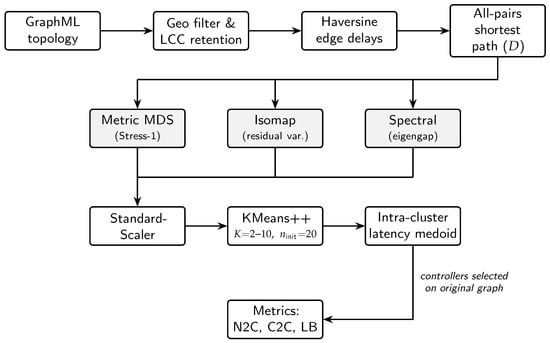
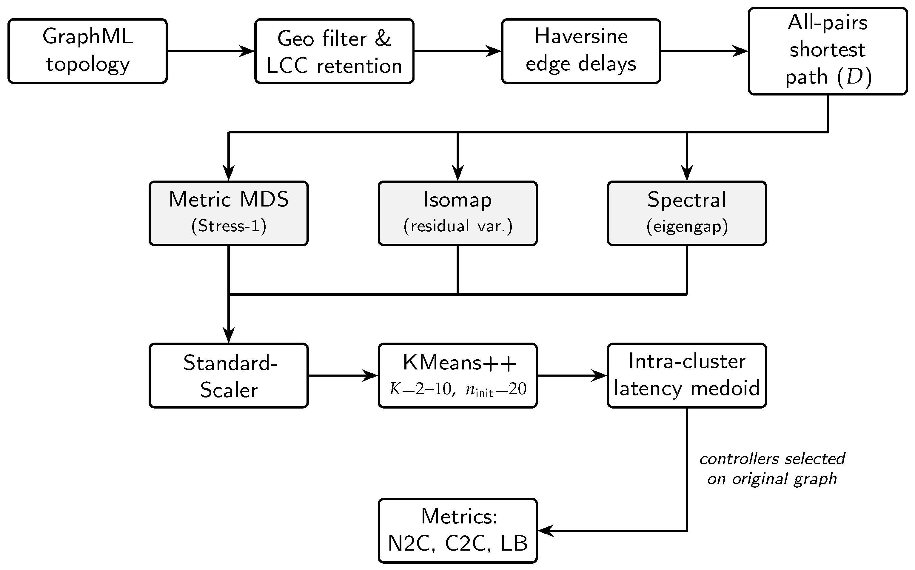
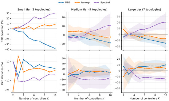
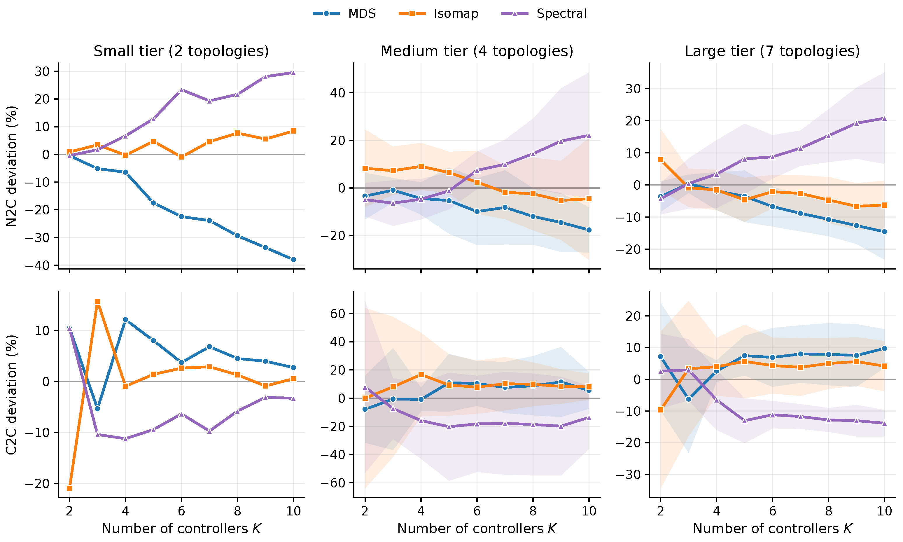
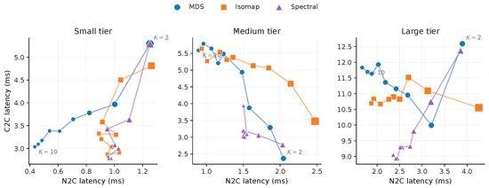
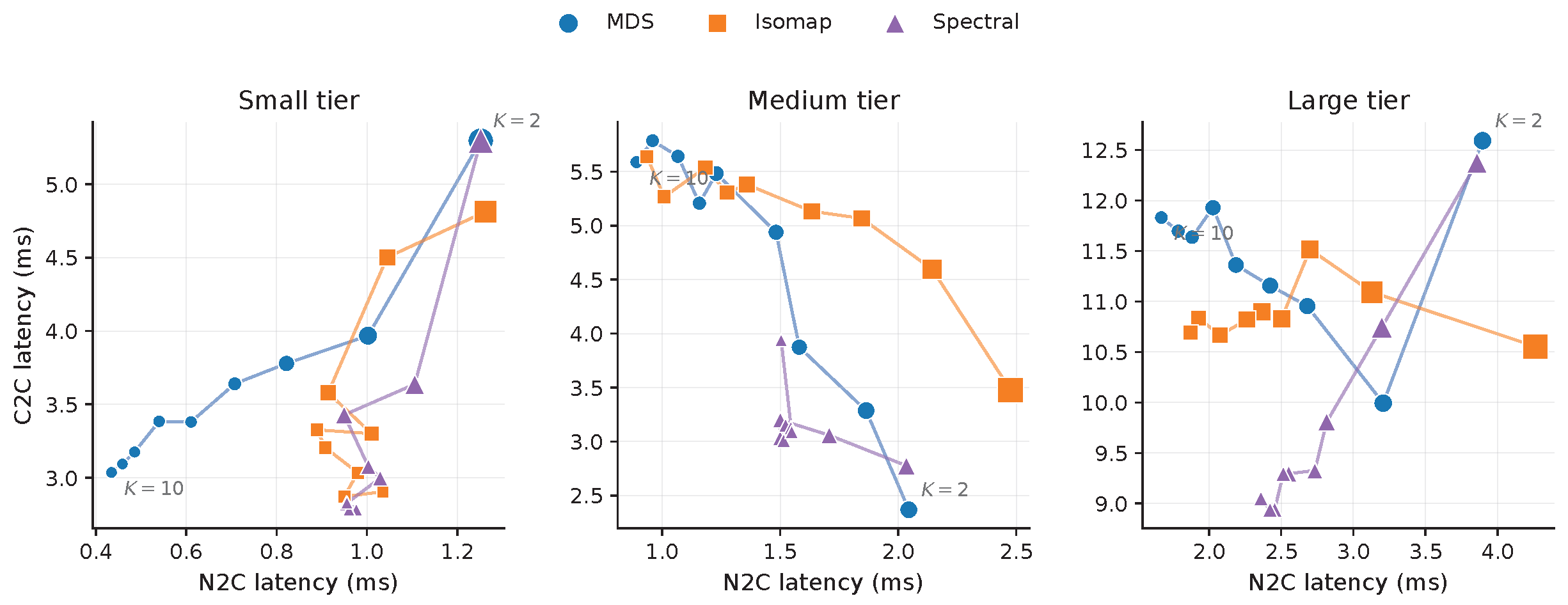

Disclaimer/Publisher’s Note: The statements, opinions and data contained in all publications are solely those of the individual author(s) and contributor(s) and not of MDPI and/or the editor(s). MDPI and/or the editor(s) disclaim responsibility for any injury to people or property resulting from any ideas, methods, instructions or products referred to in the content. |
© 2026 by the authors. Licensee MDPI, Basel, Switzerland. This article is an open access article distributed under the terms and conditions of the Creative Commons Attribution (CC BY) license.