Per-Link Path Loss Estimation Method in Low-Power Wide-Area Networks via Geographical Clustering: Experimental Results Using LoRa ^†

Abstract

Path loss modeling is essential for the design, analysis, and applications (e.g., localization) of low-power wide-area networks (LPWANs). Conventional models typically rely on coarse regional land cover classifications (e.g., urban or suburban), which fail to capture the direction-dependent path loss variations of long-range LPWAN links that traverse heterogeneous environments. Although per-link modeling and geographical clustering have individually shown promise in addressing these limitations, their combined potential remains unexplored. This paper presents GeoSeg, a path loss modeling approach that integrates per-link modeling with geographical clustering. GeoSeg represents the propagation environment between each transmitter-receiver pair as a variable-length sequence that encodes both land cover types and their spatial arrangement and employs a hidden Markov model (HMM)-based clustering method to group these sequences into subregions. A per-subregion path loss exponent is then estimated for each identified subregion, enabling spatially adaptive path loss estimation. Evaluated using an open-access LoRaWAN dataset, the preliminary results demonstrate median MAE reductions of up to 96% across the evaluated clusters compared with the standard log-distance path loss model. These results suggest that integrating per-link environmental characterization with geographical clustering can potentially improve path loss estimation accuracy in heterogeneous LPWAN deployments.

1. Introduction

IoT applications such as those in smart cities, precision agriculture, and environmental monitoring require technologies capable of long-range data transmission with minimal power consumption. Common wireless technologies such as ZigBee and Bluetooth are unsuitable for long-distance communication because of their limited range. While conventional cellular systems were historically considered unsuitable for energy-constrained IoT devices due to high power consumption [1], modern cellular networks have introduced massive Machine-Type Communication (mMTC) capabilities under the IMT-2020 framework, explicitly targeting connectivity density and energy efficiency for IoT applications, with an increasing number of connected devices expected with Beyond 5G (B5G) and 6G networks [2]. Nonetheless, LPWAN technologies continue to offer distinct advantages for applications requiring long-range connectivity combined with multi-year battery life, particularly in scenarios where cellular-based IoT deployment is economically unviable or limited by sparse cellular infrastructure.

Among the available LPWAN technologies—including Sigfox, NB-IoT, and LTE-M—long range (LoRa) has gained particular prominence in both research and industry [3]. LoRa is a proprietary chirp spread spectrum (CSS) modulation technology developed by Semtech that operates in the unlicensed sub-GHz industrial, scientific, and medical (ISM) bands [4]. Built on top of LoRa’s physical layer, the long-range wide-area network (LoRaWAN) is an open media access control (MAC) layer protocol and network architecture standardized by the LoRa Alliance [5]. In a typical LoRaWAN deployment, end devices transmit data to one or more gateways, which forward received packets to a network server for processing.

As of 2023, The Things Industries, a LoRa-based LPWAN IoT solutions provider, has reached 1 million devices connected to their network server infrastructure [6]. These millions of devices enable numerous applications that require or benefit from accurate path loss modeling. As a key component of wireless system design, path loss modeling enables coverage prediction and network planning. Since factors affecting path loss, like multipath fading and shadowing, are directly influenced by the propagation environment, land cover information becomes indispensable for accurate path loss estimation.

Although most propagation models used in LPWAN studies incorporate land cover information, they typically provide only a general description of the overall propagation area (e.g., Okumura–Hata or log-distance path loss model). Many LPWAN studies use regional modeling for path loss estimation [7,8,9,10,11], which relies on coarse environmental classifications such as urban, suburban, or rural. In this approach, all radio links within a region are modeled using the same path loss formula or propagation parameters. For example, the path loss of links in a suburban area may be estimated using the semi-urban variant of the Okumura–Hata model or the log-distance model with a path loss exponent adjusted for suburban environments. However, this regional approach produces an isotropic representation of gateway coverage, which is often incompatible with LPWAN deployments in areas with heterogeneous land cover. In practice, such heterogeneity introduces significant variability in path loss, depending on the direction of propagation.

Recent studies addressed the challenge associated with regional modeling by using a per-link approach to path loss estimation. For these studies, multi-spectral satellite images and GIS technology were used to create land cover classification maps. With granular propagation environment information, these studies then employed either of two methods: (1) creating a per-link variant of an existing propagation model [12,13] or (2) incorporating per-link data for a neural network-based path loss estimation [14].

Geographical clustering is another approach that addresses the issues related to regional models in diverse propagation environments. This approach partitions the propagation area into distinct subregions using unsupervised machine learning, with each subregion assumed to exhibit unique propagation characteristics. Per-subregion models are then developed to capture these variations.

One widely used propagation model in LPWAN studies is the log-distance path loss model. It is an empirical analytical model that offers an environment-specific parameter: the path loss exponent ($\eta$). Calibrating the log-distance path loss model primarily involves determining $\eta$. Once $\eta$ is known, the total path loss ($PL$) of a transmission at a distance (d) can be calculated using Equation (1). Here, $P{L}_0$ represents the measured path loss at the reference distance $d_0$, and $X_{\sigma }\sim \mathcal{N}(0,{\sigma }^2)$ denotes the shadowing component modeled as a zero-mean Gaussian random variable with variance ${\sigma }^2$:

$$PL=P{L}_0+10\eta log\left(d/d_0\right)+X_{\sigma }$$

(1)

This study introduces GeoSeg, a variant of the log-distance path loss model that integrates per-link modeling with geographical clustering. This proposed method was developed using an open-access LoRaWAN dataset [15]. To evaluate the performance of our proposed method, its path loss estimation accuracy was compared to the standard log-distance path loss model.

The succeeding sections of this paper are organized as follows. Section 2 presents a review of related works, surveying the existing literature relevant to the study. Section 3 details the methodology, describing the proposed approach and its theoretical foundations. Section 4 covers data exploration and preprocessing, outlining the dataset characteristics and the preparation steps applied prior to model training. Section 5 presents the results and discussion, where the experimental findings are analyzed and interpreted. Finally, Section 6 concludes the paper, summarizing the key contributions and suggesting directions for future work.

2. Review of Related Works

Accurate path loss estimation in LPWANs has motivated a range of modeling approaches that incorporate environmental information at varying levels of spatial granularity. While early studies relied primarily on regional propagation models, more recent work leverages geographic data such as satellite imagery and land cover maps to better capture environmental heterogeneity. These approaches differ in how environmental features are extracted and integrated into propagation models. This section reviews related studies with an emphasis on methods that utilize land cover information to improve path loss estimation in diverse propagation environments, particularly per-link modeling and geographical clustering.

2.1. Per-Link Path Loss Estimation

A number of studies have explored per-link approaches for LoRa-based LPWAN path loss estimation by incorporating environmental information specific to each radio link. Using land cover data derived from satellite imagery and GIS tools, these methods characterize the propagation environment along individual links to improve modeling accuracy [12,13,14].

2.1.1. Per-Link Variant of Okumura–Hata

One LoRa-based study developed per-link variants of the Okumura–Hata model [12]. Using satellite imagery, the dominant land cover type along each radio link is identified and used to determine the corresponding built-environment category. As a result, individual radio links can be classified as urban, semi-urban, or open space, depending on the dominant land cover along the link path. The appropriate Okumura–Hata formulation is then applied to estimate the path loss of each link [12]. The study showed that regional models, such as the free-space path loss model and the Bor model (a calibrated log-distance path loss model), are incompatible with diverse propagation environments, as they tend to produce overly optimistic or overly conservative estimates [12].

It is important to note that the Okumura–Hata model is assumed to be valid for frequencies between 150 MHz and 1500 MHz, base station antenna heights between 30 m and 200 m, mobile antenna heights between 1 m and 10 m, and link distances between 1 km and 20 km [16]. Most LPWAN technologies, e.g., LoRa, fall within the valid frequency range [17]. Hence, the appropriateness of using the Okumura–Hata model depends mainly on the physical deployment parameters of the base station and target nodes. Existing datasets that do not satisfy these validity ranges or do not provide the necessary system parameter information (e.g., base station antenna height and mobile antenna height) would be incompatible for evaluating the performance of the Okumura–Hata model.

2.1.2. Segmented Log-Distance Path Loss Model

Another study, SateLoc, computed the total link path loss by segmenting radio links based on land cover type and applying the log-distance model sequentially per segment, with path loss exponents calibrated from 1250 RSS field measurements across five land cover types. However, this method has two key limitations. First, representing links as single-pixel lines fails to capture attenuation from the surrounding environment, making estimates sensitive to land cover misclassifications [14]. Second, its calibration requirement that both the gateway and transmitter be located within the same land cover region [13] may limit applicability in existing deployments or datasets.

2.1.3. Neural Network-Based Modeling with 2D Radio Link

DeepLoRa, unlike SateLoc, used a 2D region (i.e., rectangular area) instead of a line to represent a radio link. This approach captures the signal attenuation caused by the surrounding land covers [14]. DeepLoRa used a bidirectional long short-term memory neural network to develop the path loss database. A large-scale measurement campaign was performed to obtain the dataset for the neural network (over 30,000 records in a span of three months). The comparison of the results of these studies, when applied in the same location, is shown in Table 1 [14]. Among these studies, DeepLoRa was most accurate, with a 3.56 dB mean path loss estimation error.

Table 1. Comparison of studies that used per-link approach for path loss estimation in LoRa.

Method	Mean Path Loss Error [dB]	Standard Deviation [dB]
per-link Okumura–Hata [12]	8.88	8.58
SateLoc [13]	15.61	12.90
DeepLoRa [14]	3.56	3.17

2.2. Geographical Clustering-Based Path Loss Modeling

Geographical clustering is another approach that addresses the limitations of regional models in diverse propagation environments. This method divides the propagation area into subregions using unsupervised machine learning, where each subregion is assumed to have distinct propagation characteristics, enabling the development of per-subregion propagation models. In an LTE network, it has been demonstrated that a site-specific geographical clustering approach can enhance path loss estimation accuracy by employing k-means clustering for subregion identification and convolutional neural networks for per-subregion modeling [18]. Notably, geographical clustering has yet to be applied in LPWAN propagation modeling studies.

Feature Development

A key design consideration in geographical clustering is how the link region is represented in the feature space. Fixed-size rectangular regions rotated along the Tx-Rx direction [19,20] do not cover the full link extent between the node and the base station. DeepLoRa improves on this by representing the full link as a rectangular area composed of sequential micro-links, each embedded as a vector of land cover proportions [14]. However, this embedding captures only the composition of land covers within each micro-link, without accounting for their spatial arrangement relative to the line of sight.

2.3. Research Gaps and Motivation

Across these studies, a clear progression is evident: from regional models that apply uniform parameters across the entire propagation area to per-link methods that account for land cover conditions along individual links and geographical clustering approaches that enable localized modeling through subregion partitioning. Despite these advances, no existing study has combined per-link modeling and geographical clustering for LoRa path loss estimation, and existing link region representations do not fully capture the 2D spatial arrangement of land covers relative to the propagation path. This work addresses these gaps by proposing a log-distance path loss model that integrates per-link environmental characterization with geographical clustering, underpinned by a link region representation that captures the 2D spatial distribution of land covers along the propagation path, enabling spatially adaptive path loss estimation for LoRa networks in diverse land cover environments.

3. Methodology

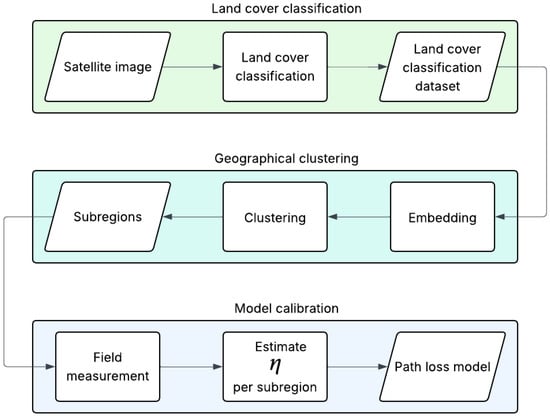
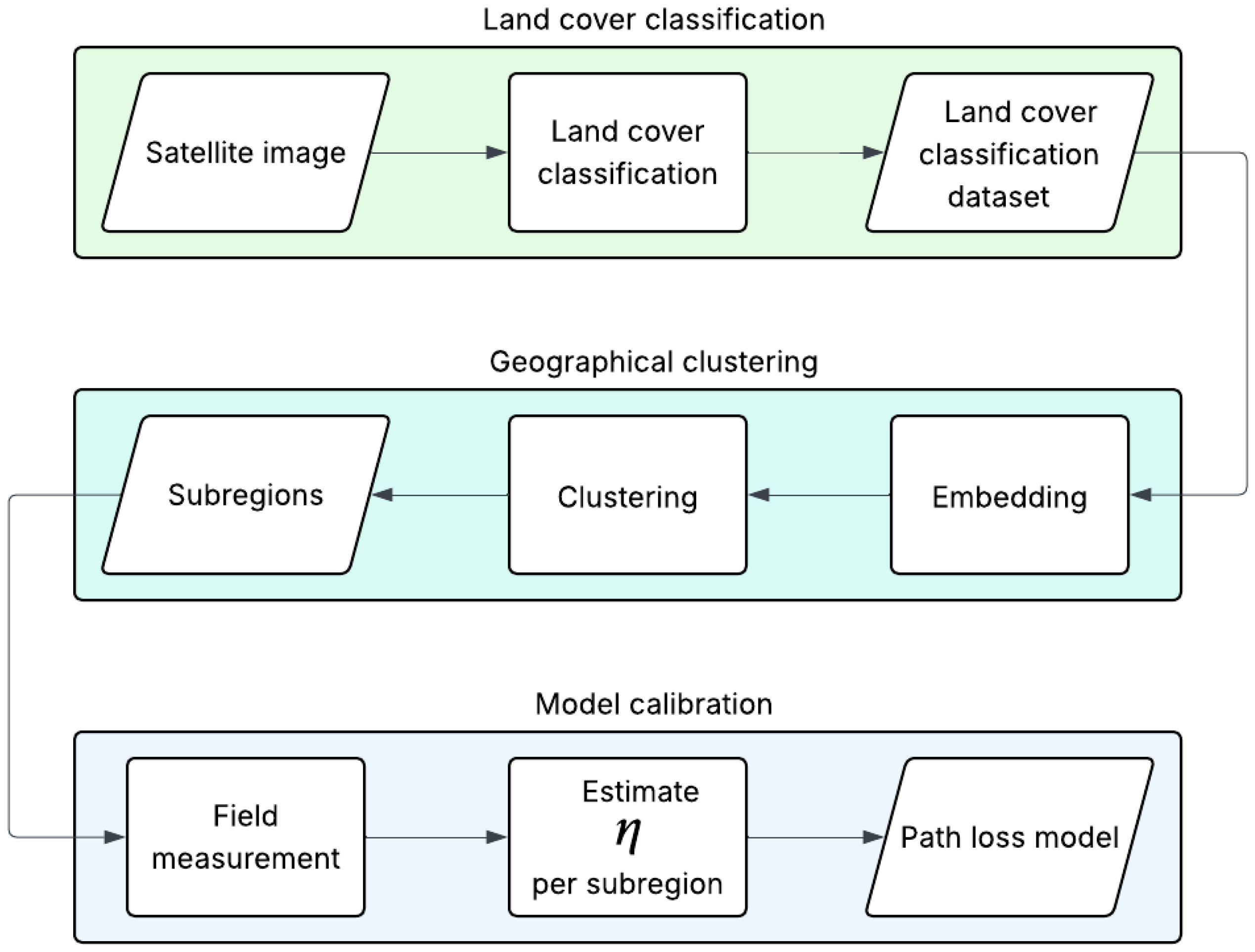
The development of GeoSeg comprised three main processes: land cover classification, geographical clustering, and model calibration. Figure 1 shows the path loss model development process. Multi-spectral satellite imagery and GIS data were employed for land cover classification. For geographical clustering, this study developed an embedding method—which generated features from each radio link’s propagation region—and utilized a hidden Markov model-based clustering approach. Finally, model calibration involved taking field measurements and using these to determine the path loss exponent for each subregion. The succeeding three sections—Section 3.1, Section 3.2 and Section 3.3—discuss each of these processes in detail.

Figure 1. Path loss model development process using the proposed method.

3.1. Land Cover Classification

The area of study was located in Antwerp, Belgium, where the dataset [15] for the path loss model calibration was collected. It was a 4.2 km × 2.6 km region bounded by the lower-left and upper-right coordinates 51.192966° N, 4.388045° E and 51.231055° N, 4.425235° E, respectively. The identification process of the area of study is detailed in Section 3.3.1.

The area comprised five main land cover types: buildings, trees, open fields, roads, and water. The multi-spectral image was obtained from the Copernicus Sentinel-2 database and filtered for the period from 1 January 2019 to 31 December 2019. The spectral bands used for the classification were B2 (blue, 490 nm), B3 (green, 560 nm), B4 (red, 665 nm), B5 (vegetation red edge, 704 nm), B6 (vegetation red edge, 740 nm), B7 (vegetation red edge, 783 nm), and B8 (near-infrared, 832 nm). Additionally, the normalized difference vegetation index (NDVI) was derived from the near-infrared and red bands (i.e., B8 and B4, respectively).

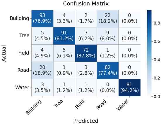
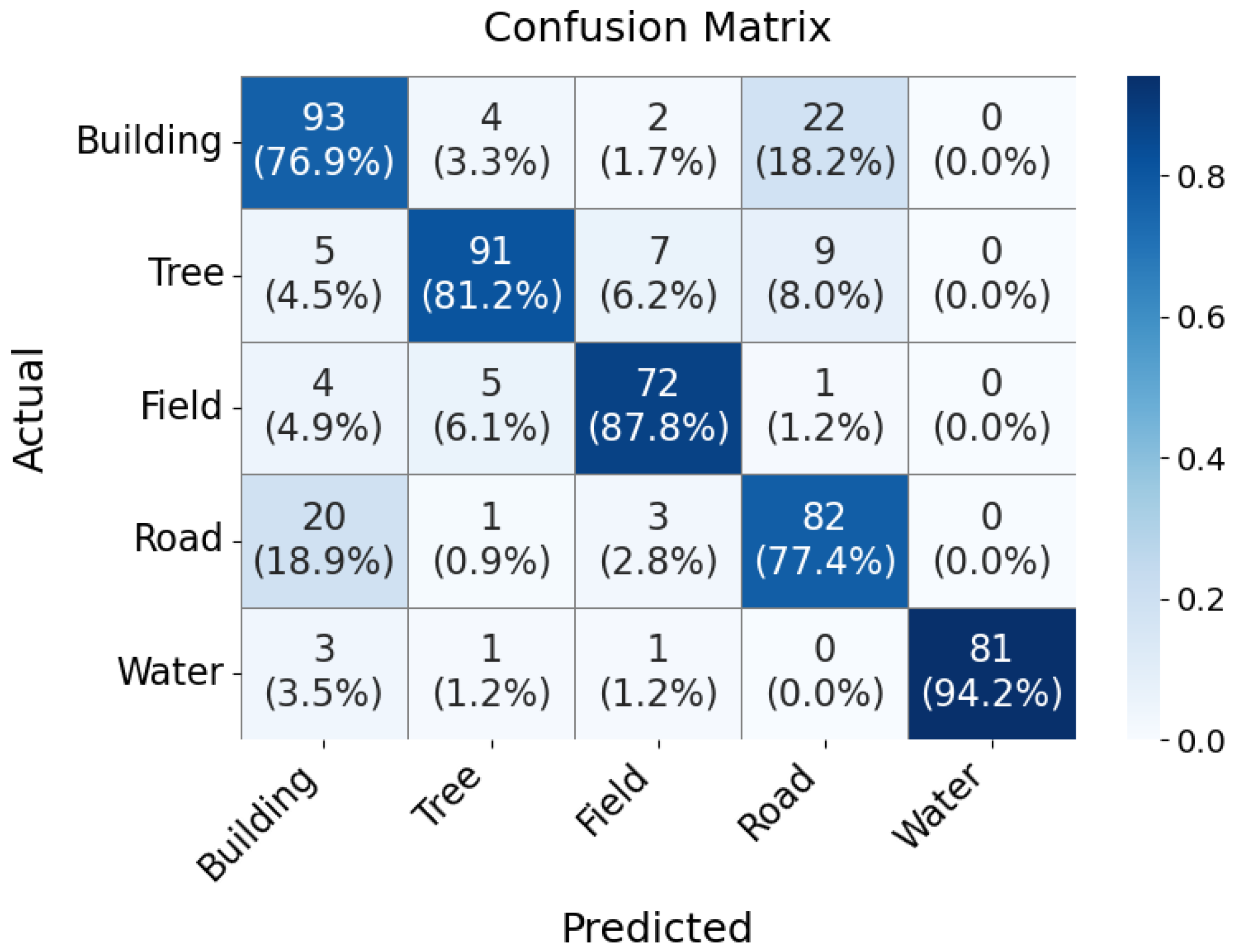
Google Earth Engine (GEE) was used for land cover classification. Training and validation cells were manually labeled, with the following distribution: 552 buildings, 513 trees, 504 fields, 517 roads, and 520 water, totaling 2606 data points. Of these, 80% of the dataset was used for training, and the remaining 20% was reserved for validation. GEE offers four built-in classifiers: random forest, naive Bayes, CART, and SVMs. Among these, the random forest classifier achieved the highest overall classification accuracy of 83% for this study’s dataset. The confusion matrix for the validation dataset is shown in Figure 2, and Table 2 shows the classification performance metrics.

Figure 2. Land cover classification confusion matrix.

Table 2. Precision, recall, and F1 score per class.

Class	Precision	Recall	F1 Score
Building	0.7440	0.7748	0.7591
Tree	0.8824	0.8208	0.8505
Field	0.8471	0.8780	0.8622
Road	0.7193	0.7736	0.7455
Water	1.0000	0.9419	0.9701
Macro Avg	0.8386	0.8378	0.8375
Weighted Avg	0.8364	0.8354	0.8354

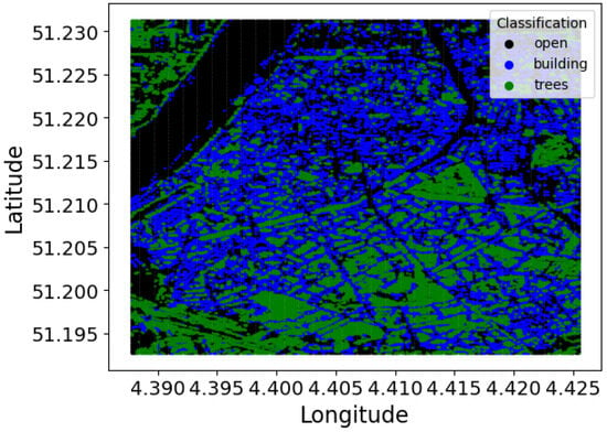
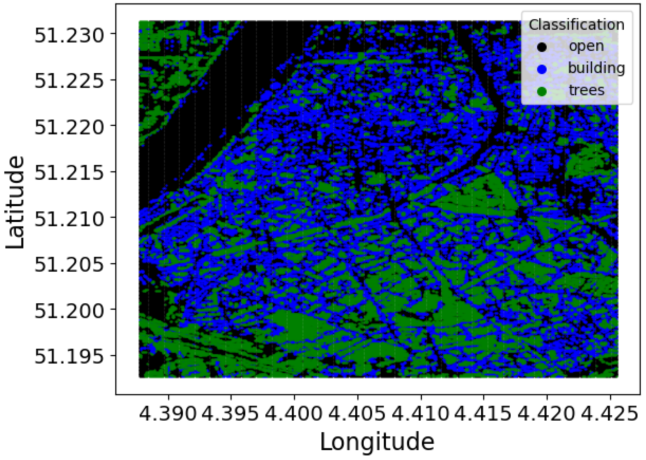
The resulting land cover classification map had a resolution of 10 m × 10 m, matching the cell resolution of the multi-spectral image. Figure 3 is the visualization of the land cover classification. The field, road, and water classes were collectively labeled as open.

Figure 3. Land cover classification of the study area.

3.2. Geographical Clustering

Every cell in the land cover classification map was assigned to a cluster. This assignment involved two main steps: (1) embedding the land cover information of the 2D propagation region between the cell and the gateway and (2) performing clustering. In this study, the gateway was located at 51.197458° N, 4.406731° E. The identification and details of this gateway are discussed in Section 3.3.1.

3.2.1. Embedding

The proposed methodology transforms the two-dimensional propagation region between a cell and the gateway into a feature vector suitable for clustering analysis. The region, characterized by a width w and length n, is converted into a vector $\mathbf{v}\in {\mathbb{R}}^{wn}$ through an embedding process that captures the following characteristics of the propagation environment: land cover types and their positions relative to the line-of-sight (LoS) path.

Each cell $(i,j)$ within the propagation region is assigned a value ${\omega }_{ij}$ that quantifies its impact on signal propagation, which is calculated as follows:

$${\omega }_{ij}={\lambda }_{ij}\times c_{ij}$$

(2)

where ${\lambda }_{ij}$ represents the position-dependent weight and $c_{ij}$ denotes the land cover classification. The land cover types are numerically encoded as follows:

$$c_{ij}=\left\{\begin{array}{cc}0\hfill & (\mathrm{open}\mathrm{space}:\mathrm{fields},\mathrm{roads},\mathrm{water})\hfill \\ 1\hfill & \left(\mathrm{trees}\right)\hfill \\ 2\hfill & \left(\mathrm{buildings}\right)\hfill \end{array}\right.$$

(3)

The positional weight ${\lambda }_{ij}$ is determined by the cell’s distance from the central LoS path, located at column $j=\lfloor w/2\rfloor$.

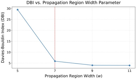
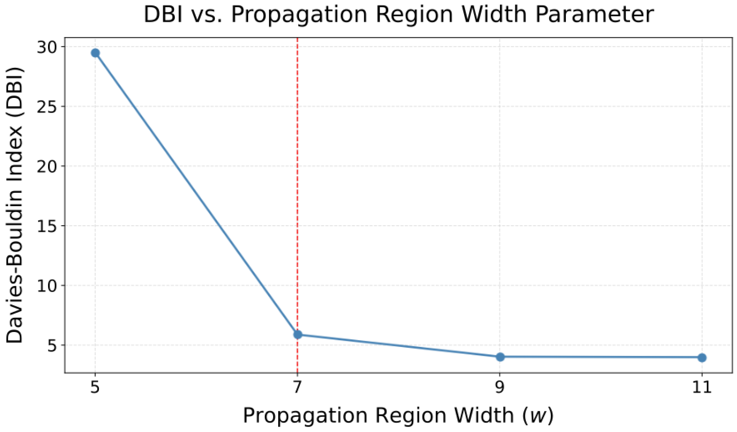
The propagation region width $w=7$ used throughout this study was initially adapted from [14], which employed the same 2D spatial representation. To validate this choice, a grid search over $w\in \{5,7,9,11\}$ was conducted, with clustering quality evaluated using the Davies–Bouldin index. The evaluation was conducted on a small portion of the study area around the gateway, following the clustering process (Steps 1–5) described in Section 3.2.2. As shown in Figure 4, $w=7$ yielded the largest marginal reduction, making it a reasonable choice. With a width $w=7$, the LoS lies at $j=3$. The weights decrease symmetrically with distance from the LoS:

$${\lambda }_{ij}=⌊{\displaystyle \frac{w}{2}}⌋+1-\left|j-⌊{\displaystyle \frac{w}{2}}⌋\right|$$

(4)

yielding discrete values of ${\lambda }_{ij}\in \{1,2,3,4\}$, as shown in

$${\lambda }_{ij}=\left\{\begin{array}{cc}1,\hfill & j=0,6\hfill \\ 2,\hfill & j=1,5\hfill \\ 3,\hfill & j=2,4\hfill \\ 4,\hfill & j=3\hfill \end{array}\right.$$

(5)

Figure 4. Davies–Bouldin indices at various propagation widths w, showing w = 7 having the largest marginal improvement.

Using Equation (2), the resulting ${\omega }_{ij}$ values for different land cover types and positions are shown in Equation (6). Note that at $c=0$, $\omega$ is always 0 because it is assumed that open spaces do not obstruct the signal:

$${\omega }_{ij}\in \left\{\begin{array}{cc}\left\{0\right\},\hfill & c=0\hfill \\ \{1,2,3,4\},\hfill & c=1\hfill \\ \{2,4,6,8\},\hfill & c=2\hfill \end{array}\right.$$

(6)

The final feature vector $\mathbf{v}$ is created by flattening the $n\times w$ matrix of ${\omega }_{ij}$ values using

$$v\left[k\right]={\omega }_{ij}\mathrm{where}k=w·i+j$$

(7)

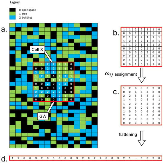
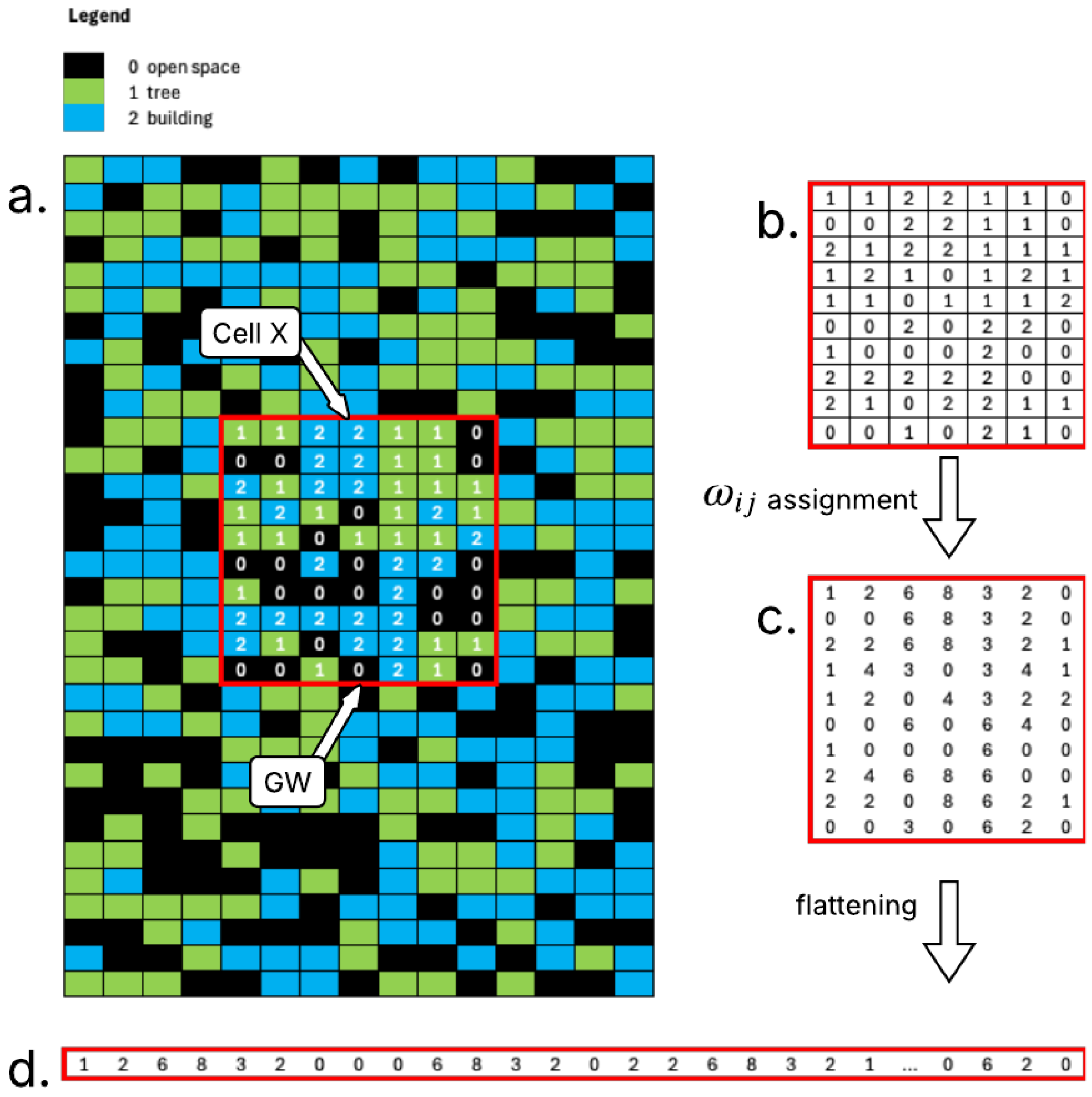
for $i\in \{0,\dots ,n-1\}$ and $j\in \{0,\dots ,w-1\}$. These feature vectors serve as inputs for the clustering algorithm, preserving both the land cover information and its spatial context relative to the propagation path. Figure 5 shows a sample embedding process to create the feature vector of the propagation region between the gateway (GW) and a cell X.

Figure 5. Embedding process visualization: (a) propagation region between gateway (GW) and cell X, (b) raw land cover data, (c) weighted cells (${\omega }_{ij}$ values), and (d) flattened feature vector $\mathbf{v}$.

3.2.2. Clustering

Due to the variable lengths of propagation regions, the corresponding feature vectors produced by the embedding process exhibited differing dimensionalities. This necessitated the use of a clustering method capable of handling variable-length inputs, which is a common challenge in sequential data analysis [21]. Distance-based clustering methods compute pairwise dissimilarities between sequences to construct a distance matrix, from which clustering algorithms can be applied [22]. Among the most widely used dissimilarity measures for variable-length sequence clustering are dynamic time warping, edit distance (Levenshtein distance), and longest common subsequence [23]. However, these methods have inherent quadratic time and space complexity in sequence length, i.e., $O(T_1\times T_2)$ per pairwise computation [24,25,26]; they additionally require $O\left(N^2\right)$ computations to construct the full distance matrix for N sequences, rendering them computationally expensive at scale. An alternative for handling large datasets is feature-based methods [22]. These methods map variable-length sequences into fixed-size vectors prior to clustering. Among these are deep learning-based approaches, such as autoencoder-based clustering, which use a neural network encoder to transform variable-length sequences into fixed-length representations and then apply a standard clustering algorithm to these representations [27]. However, this approach introduces significant architectural complexity and hyperparameter tuning requirements, such as the dimension of the fixed-length representation, the number of layers, and the number of neurons, which may require trial and error or grid searching to find optimal values [28].

This study employs a model-based approach, specifically a hidden Markov model (HMM)-based clustering method [29] which was modified to reduce computational burden for large datasets. This modification addresses the scalability limitation of distance-based methods while avoiding the architectural complexity of deep learning-based approaches. To illustrate this method, consider a dataset D with N sequences $\{X_1,\dots ,X_N\}$ of emissions (observed states) with varying lengths. The following steps describe the modified clustering procedure:

Step 1.

Randomly sample n sequences from the dataset D to create a reduced-sized dataset d of a size n.

Step 2.

Fit an HMM $m_i$ for each sequence $x_i\in d$, $1\le i\le n$.

Step 3.

For each fitted model $m_i$ and sequence $x_j$, evaluate the log-likelihood $L\left(x_j\right|m_i)$, $1\le i,j\le n$. The log-likelihoods are used to define pairwise distances of sequences $x_i$ and $x_j$ [29].

Step 4.

Create a distance matrix A. The elements $a_{ij}$ of A are equal to ${\displaystyle \frac{1}{2}}(L\left(x_j\right|m_i)+L\left(x_i\right|m_j))$.

Step 5.

Apply a hierarchical clustering algorithm to generate K clusters from the distance matrix A.

Step 6.

Having clustered the sequences into K groups, fit K HMMs $\{M_1,...,M_K\}$, with one for each cluster.

Step 7.

For each sequence $X_l\in D$, assign its cluster $k\in \{1,2,...,K\}$ by solving $k=\underset{M_k}{argmax}L\left(X_l\right|M_k)$.

With $n\ll N$, the distance matrix A in Step 4 is $n\times n$ rather than the $N\times N$ matrix required by direct distance-based clustering, reducing matrix construction from $O\left(N^2\right)$ to $O\left(n^2\right)$ and substantially lowering both the memory and computational cost.

Having established the clustering procedure, the remaining implementation details concern the configuration of the HMM itself. In this study, the number of observed states was set to seven, corresponding to the seven discrete values of $\omega$ described in Section 3.2.1. The number of hidden states was set to three based on domain knowledge of the propagation environment. Since the propagation environment consisted of three distinct land cover types, a three-state HMM was deemed a reasonable model complexity for capturing the underlying structure of the sequences. A more rigorous selection of the optimal number of hidden states is left for future work. Finally, to fit an HMM to a sequence of observed states, this study utilized the hmmlearn Python 3.9 package [30], with its emission model set to Categorical with randomly initialized model parameters, and the Baum–Welch algorithm for model training.

Identifying the Optimal Number of Clusters 

The Davies–Bouldin score was used to determine the optimal number of clusters. This score is calculated as the average similarity of each cluster with its most similar cluster, where similarity is defined as the ratio of intra-cluster distances to inter-cluster distances. Consequently, well-separated (farther apart) and compact (less dispersed) clusters yield better scores. Lower values indicate better clustering, and the minimum score is zero.

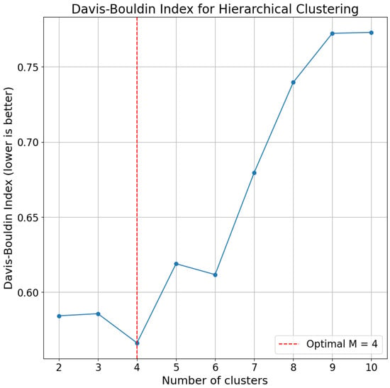
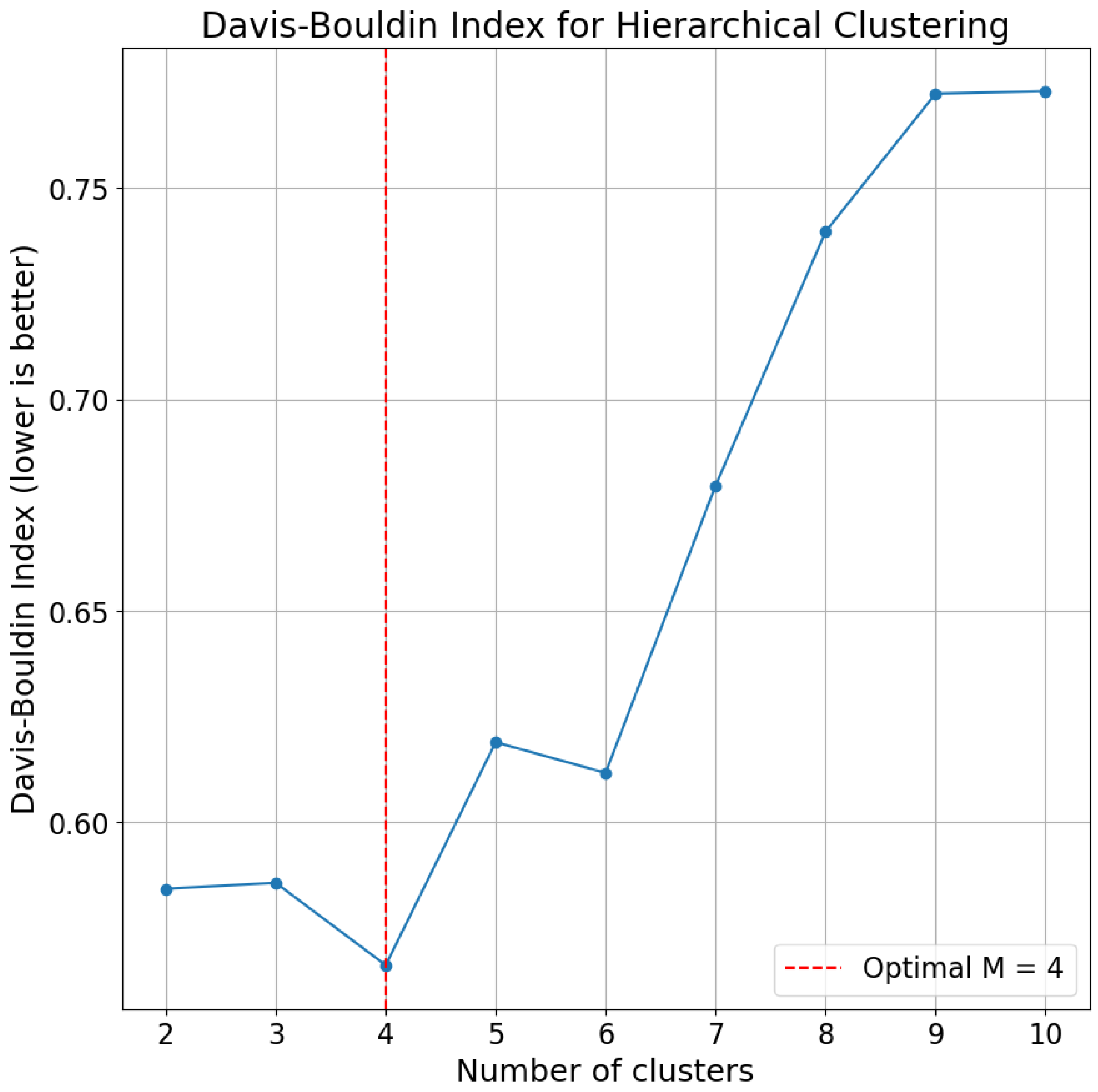
To identify the optimal K, Steps 1–5 of Section 3.2.2 were repeated for different values of K, and the corresponding Davies–Bouldin score was recorded. The built-in davies_bouldin_score implementation of Python’s Scikit Learn package was used for this. Figure 6 displays the scores for $K\in \{2,3,\dots ,10\}$, indicating that the optimal number of clusters was four ($K=4$).

Figure 6. Davies–Bouldin indices at various number of clusters, showing K = 4 as optimal.

Interpretation of the Clusters 

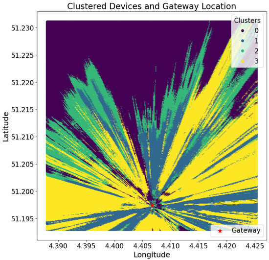
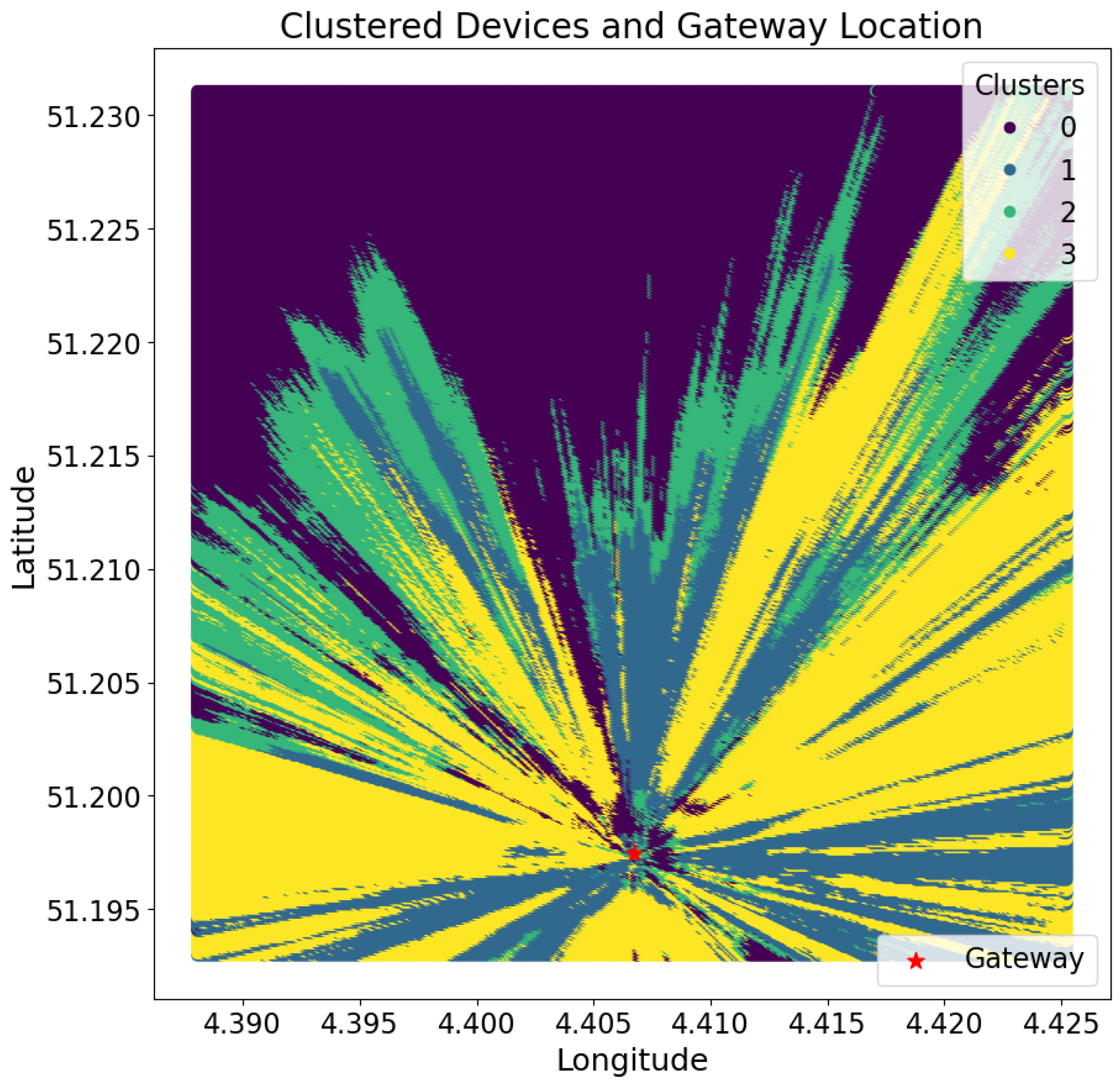
The visualization of the clusters is shown in Figure 7. To interpret the clustering results, two observable parameters were used. The first was the land cover distribution of the propagation regions within each cluster, which captures the aggregated proportions of land cover types—namely buildings, trees, and open space—across all propagation regions assigned to a given cluster. This metric reflects the dominant environmental composition characterizing the propagation regions in each cluster. The second parameter was the probability distribution of the land covers by distance from the line of sight, which indicates how the presence of each land cover type changes with increasing perpendicular distance from the line of sight. These parameters could provide a characterization of the spatial and environmental features associated with each cluster.

Figure 7. Visualization of the clusters at $K=4$.

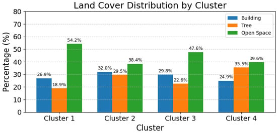
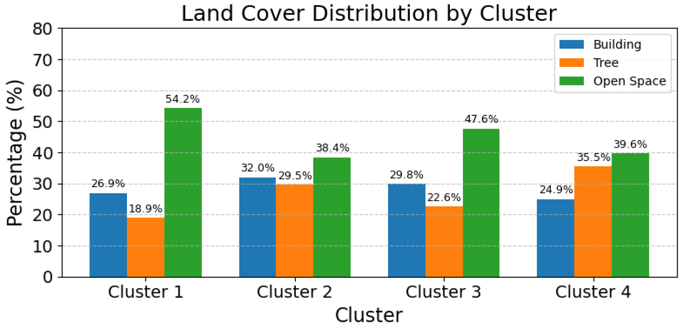
Figure 8 illustrates the distribution of the land cover types, namely buildings, trees, and open space, across the propagation regions represented in the clusters. Overall, open space constituted a large portion of the land cover, while buildings and trees contributed varying shares, depending on the environment. In certain cases, the distribution was relatively balanced, with buildings, trees, and open space occupying comparable proportions (e.g., Cluster 2). In other regions, a particular land cover type became more dominant, such as higher tree presence (e.g., Cluster 4: 35.5%) or extensive open areas (around 47–54%, Clusters 1 and 3), highlighting the diversity of propagation environments captured by the clustering process.

Figure 8. Land cover distribution (%) for each cluster.

On the other hand, the spatial arrangement of land cover types relative to the line of sight did not differ significantly across the clusters. The line of sight corresponded to $d=0$, and given a total width of $w=7$, the maximum perpendicular distance from the line of sight was $d=3$ cells in either direction. Table 3 presents the probability distributions of each land cover type at varying distances from the line of sight for each cluster.

Table 3. Probability distributions by distance d from the line of sight for each cluster.

Cluster	Land Cover	$\mathit{d}=3$	$\mathit{d}=2$	$\mathit{d}=1$	$\mathit{d}=0$	$\mathit{d}=1$	$\mathit{d}=2$	$\mathit{d}=3$
1	Building	0.141	0.140	0.141	0.143	0.145	0.144	0.146
	Tree	0.144	0.143	0.142	0.142	0.142	0.143	0.143
	Open	0.143	0.144	0.144	0.143	0.142	0.142	0.141
2	Building	0.137	0.142	0.144	0.146	0.148	0.145	0.138
	Tree	0.155	0.148	0.138	0.133	0.134	0.141	0.150
	Open	0.138	0.140	0.145	0.148	0.145	0.142	0.141
3	Building	0.144	0.143	0.143	0.143	0.143	0.142	0.142
	Tree	0.145	0.144	0.143	0.141	0.142	0.142	0.144
	Open	0.141	0.142	0.143	0.143	0.143	0.144	0.143
4	Building	0.144	0.149	0.146	0.142	0.139	0.140	0.140
	Tree	0.142	0.141	0.144	0.145	0.145	0.143	0.140
	Open	0.143	0.141	0.140	0.141	0.144	0.145	0.147

These distributions suggest that the clusters were not characterized by systematic differences in how land cover types were positioned relative to the line of sight. For example, buildings or trees were not consistently located closer to or farther from the line of sight in one cluster compared with another. Instead, the primary distinguishing feature among clusters appears to be the overall proportions of each land cover type within the propagation regions, as reflected in the land cover composition of each cluster.

To summarize, geographical clustering consists of two main steps: embedding and clustering. In the embedding step, the 2D propagation regions between each cell in the area of study and the gateway were transformed into feature vectors suitable for clustering. These feature vectors were composed of weighted values that accounted for both the land cover types and their spatial positions within the propagation region. For the clustering step, a hidden Markov model (HMM)-based method was employed, which is well suited for handling large datasets with variable-length feature vectors. Notably, analysis of the resulting clusters revealed that they were primarily distinguished by differences in land cover composition, while the spatial distribution of land covers with respect to the line of sight remained uniform across all clusters.

3.3. Model Calibration

3.3.1. Field Measurement

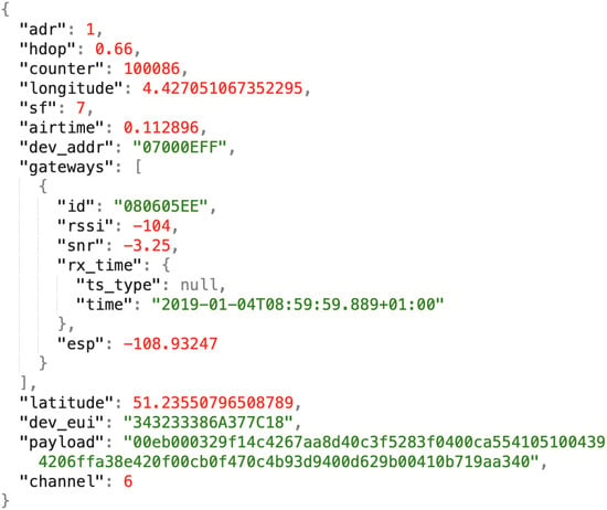
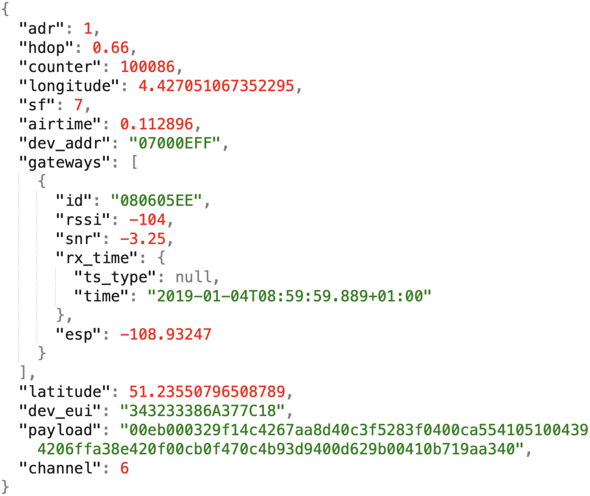
The calibration of GeoSeg requires field measurement. In this study, the field measurement data were obtained from an open-access LoRaWAN dataset collected in an urban area of Antwerp, Belgium [15]. This dataset was selected from other open-access LoRa-based datasets [31,32,33] not only for its scale and land cover appropriateness of the deployment area but, more importantly, because it provides geo-tagged transmissions and the exact geographical coordinates of the gateways, both of which were indispensable for this study. The most recent dataset version (v1.3, July 2019)—which includes the coordinates of the LoRaWAN gateways—was used in this study. Each transmission originated from one of 23 IM880B-L radio modules installed on a vehicle in Antwerp’s postal service fleet [15]. Each dataset entry contained GPS information (longitude, latitude, and HDOP) along with network parameters such as the RSSI, spreading factor, time of arrival, and receiving gateway IDs. The dataset was stored in JSON format, with Figure 9 illustrating a sample entry.

Figure 9. A sample data entry in the Antwerp dataset.

Gateway Selection and Area of Study 

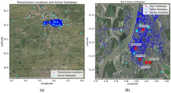
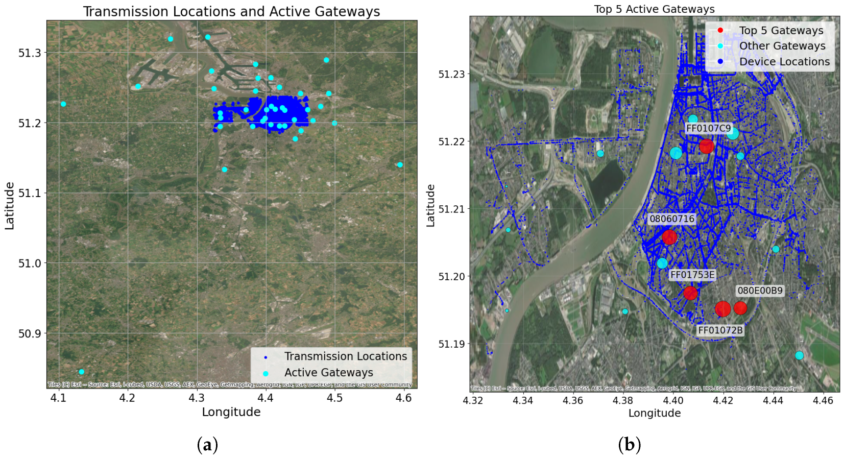
The Antwerp dataset comprises 39 active gateways and 130,430 transmissions. Figure 10a shows the spatial distribution of the gateways and transmission locations. Notably, although the gateway locations cover a large geographic region, transmissions are densely clustered in specific areas. This results in a non-uniform distribution of received transmissions per gateway, with some gateways receiving fewer than five transmissions and others exceeding 20,000.

Figure 10. (a) Spatial distribution of the active gateways and transmissions. (b) Most active gateways.

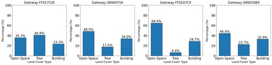
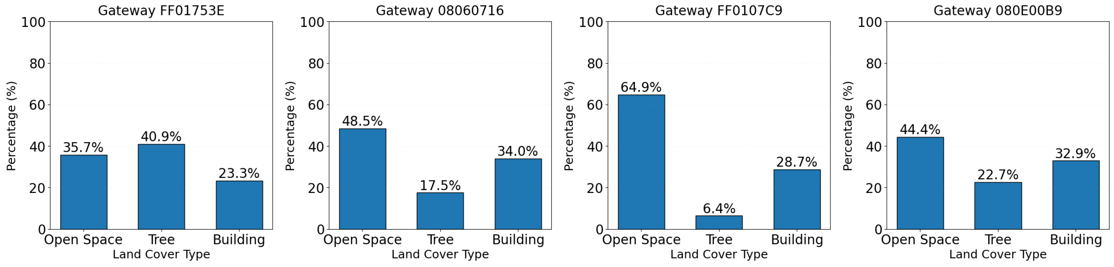
To develop GeoSeg, a gateway was selected based on its activity level and its surrounding land cover diversity. Figure 10b shows the locations of the five most active gateways, i.e., ones that had the highest receive transmission volume. For the land cover diversity, a gateway with uniform distribution of land cover classes is desired. The selected gateway (ID: FF01753E) was among the most active gateways and exhibited greater heterogeneity in its surrounding land covers, as shown by the relatively uniform distribution of land cover classes in Figure 11. This gateway received 28,529 transmissions.

Figure 11. Land cover frequency distribution of each most active gateway.

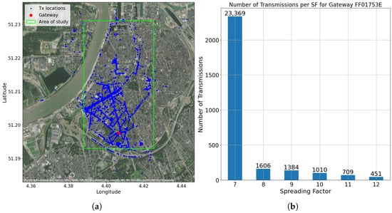
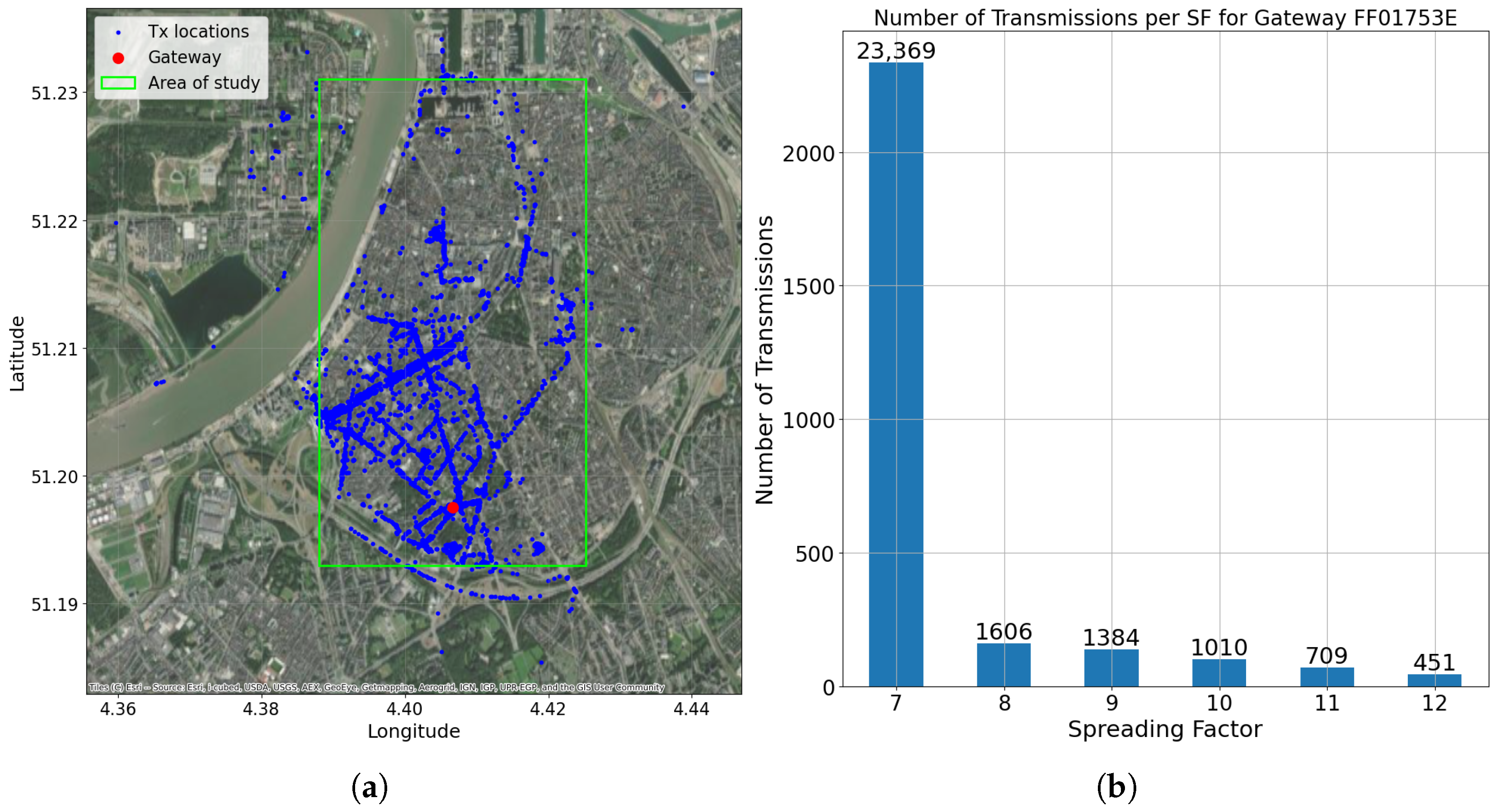
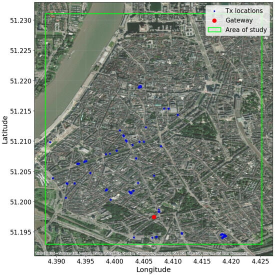
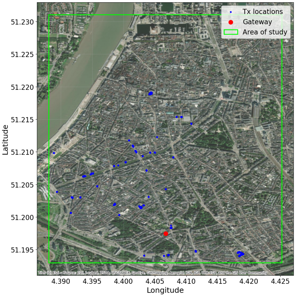
For this study, only the transmissions with a spreading factor of seven (SF7) were included since they were the most numerous (see Figure 12b). Also, all transmissions with HDOP > 5 (indicating low GPS accuracy) were removed from the dataset. This yielded a refined dataset of 22,912 entries. Figure 12a illustrates the study area, showing the spatial distribution of transmissions relative to the gateway location.

Figure 12. (a) Transmission locations and gateway located at coordinates 51.1974874° N and 4.406706° E. (b) Number of received transmissions per spreading factor for selected gateway FF01753E.

3.3.2. Estimating $\eta$

The log-distance path loss model (Equation (1)) is an empirical analytical model widely used in LoRa studies, offering an environment-specific parameter: the path loss exponent $\left(\eta \right)$. The calibration of the log-distance path loss model mainly requires determining the value of $\eta$. Since the radio link was assumed to travel through a uniform propagation environment, only a single $\eta$ needed to be estimated in Equation (1).

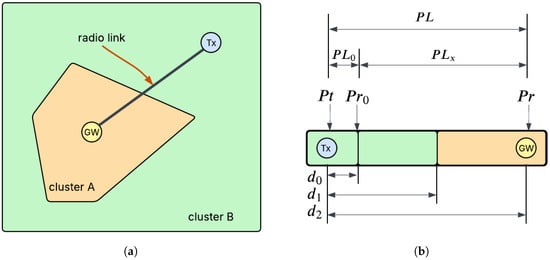
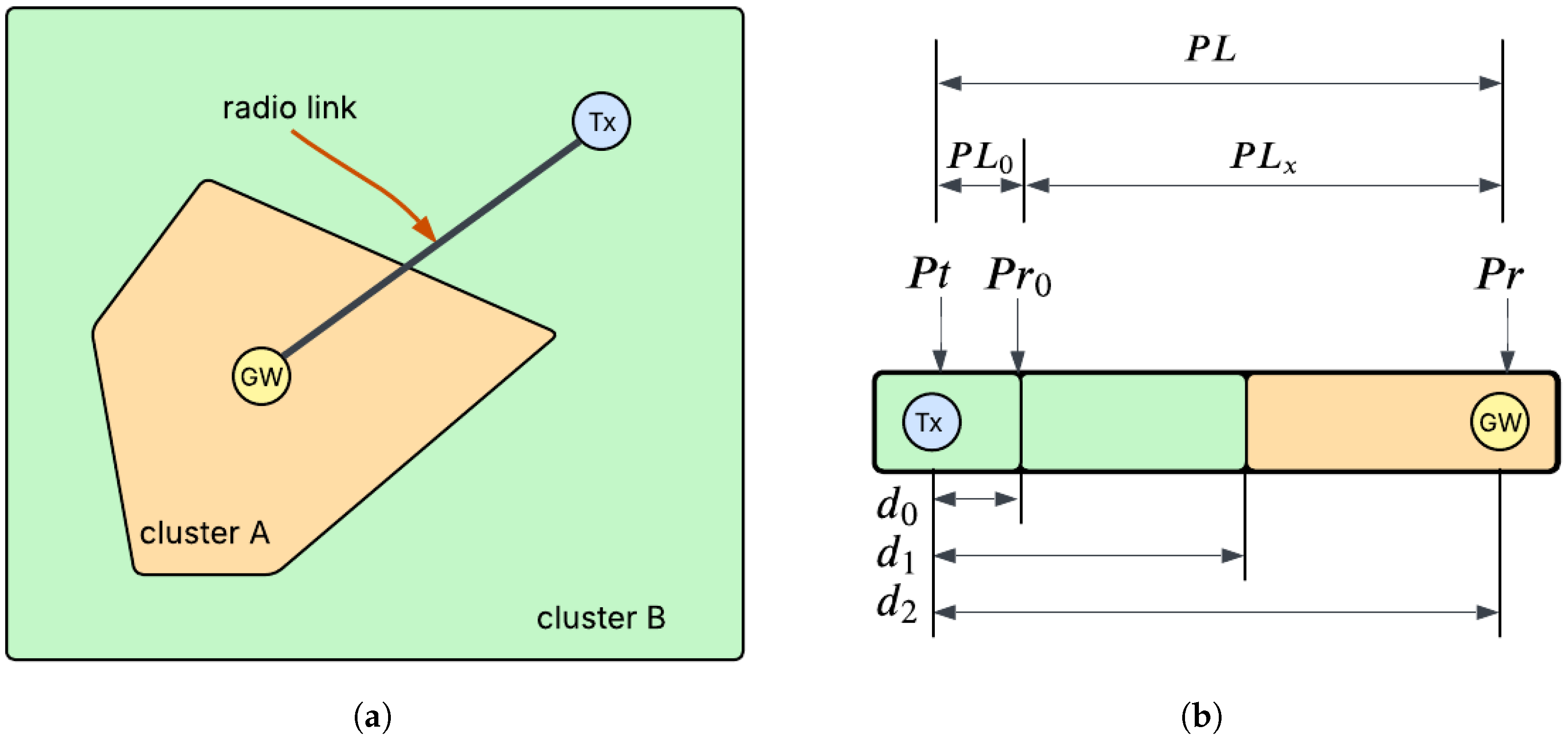
In GeoSeg, the radio link between the transmitter and receiver is modeled as a sequence of segments, each corresponding to a distinct subregion. This segmented representation requires a reformulation of the standard log-distance path loss model. A simple scenario used to derive this formulation is depicted in Figure 13a, while Figure 13b illustrates the resulting segments along the radio link between $T_x$ and $R_x$. The succeeding parts of this section describe the process of estimating the path loss exponent $\eta$, which was discussed in a previous work [34].

Figure 13. (a) Simple scenario where a radio link (propagation region) region traverses two subregions, (b) Segments and parts of a radio link. Adapted from [34].

In the scenario illustrated in Figure 12, the radio link is divided into two segments, each representing a distinct traversed subregion. The corresponding $P{L}_x$ is given by

$$P{L}_x=10{\eta }_{A}log\left({\displaystyle \frac{d_1}{d_0}}\right)+10{\eta }_{B}log\left({\displaystyle \frac{d_2}{d_1}}\right)$$

(8)

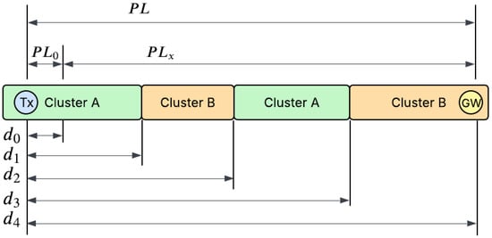
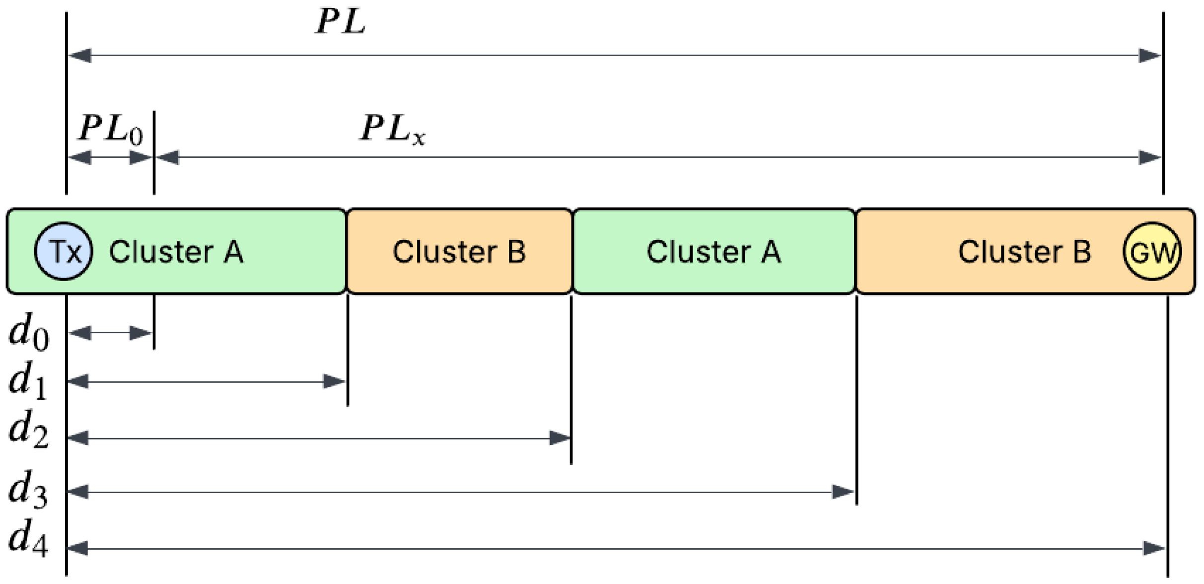
To demonstrate a more complex scenario, Figure 14 presents a case with four segments and repeating clusters. Consequently, $P{L}_x$ takes the form

$$P{L}_x=10{\eta }_{A}log\left({\displaystyle \frac{d_1}{d_0}}\right)+10{\eta }_{B}log\left({\displaystyle \frac{d_2}{d_1}}\right)+10{\eta }_{A}log\left({\displaystyle \frac{d_3}{d_2}}\right)+10{\eta }_{B}log\left({\displaystyle \frac{d_4}{d_3}}\right)$$

(9)

Figure 14. A more complicated case where subregions are traversed multiple times. Adapted from [34].

By consolidating terms from identical clusters and introducing the distance ratio $D_{(·)}$, the expression becomes

$$\begin{array}{cc}\hfill P{L}_x& =10{\eta }_{A}log\left({\displaystyle \frac{d_1{d}_3}{d_0{d}_2}}\right)+10{\eta }_{B}log\left({\displaystyle \frac{d_2{d}_4}{d_1{d}_3}}\right)\hfill \\ \hfill & =10{\eta }_{A}log\left(D_A\right)+10{\eta }_{B}log\left(D_B\right)\hfill \end{array}$$

(10)

The general expression for $P{L}_x$ with n segments and K clusters in $C=\{c_1,c_2,...,c_K\}$ is given in Equation (11), with $D_1,D_2,\dots ,D_K$ representing the distance ratio features as defined in Equation (10):

$$\begin{array}{cc}\hfill P{L}_x& =10{\eta }_{c\in C}log\left({\displaystyle \frac{d_1}{d_0}}\right)+10{\eta }_{c\in C}log\left({\displaystyle \frac{d_2}{d_1}}\right)+\dots +10{\eta }_{c\in C}log\left({\displaystyle \frac{d_n}{d_{n-1}}}\right)\hfill \\ \hfill & =10{\eta }_{c_1}log\left(D_1\right)+10{\eta }_{c_2}log\left(D_2\right)+\dots +10{\eta }_{c_k}log\left(D_K\right)\hfill \end{array}$$

(11)

Once the distance ratios have been determined, the estimation of the path loss exponent for each subregion becomes readily achievable. Equation (11) can be cast as a linear regression model $\mathit{y}=\mathit{X}\mathsf{\beta }+ϵ$, in which $ϵ$ represents the residual vector and the distance ratios $D_1,D_2,\dots ,D_K$ are features added to the dataset. Considering a training dataset of a size p, the vectors and matrix $\mathit{y}$, $\mathsf{\beta }$, and $\mathit{X}$ are given by

$$\mathit{y}=\left[\begin{array}{c}P{L}_X^{\left(1\right)}\\ P{L}_X^{\left(2\right)}\\ ⋮\\ P{L}_X^{\left(p\right)}\end{array}\right] \mathsf{\beta }=\left[\begin{array}{c}{\eta }_{c_1}\\ {\eta }_{c_2}\\ ⋮\\ {\eta }_{c_K}\end{array}\right] \mathit{X}=\left[\begin{array}{cccc}10log\left(D_1^{\left(1\right)}\right)& 10log\left(D_2^{\left(1\right)}\right)& \dots & 10log\left(D_K^{\left(1\right)}\right)\\ 10log\left(D_1^{\left(2\right)}\right)& 10log\left(D_2^{\left(2\right)}\right)& \dots & 10log\left(D_K^{\left(2\right)}\right)\\ ⋮& ⋮& \ddots & ⋮\\ 10log\left(D_1^{\left(p\right)}\right)& 10log\left(D_2^{\left(p\right)}\right)& \dots & 10log\left(D_K^{\left(p\right)}\right)\end{array}\right]$$

(12)

$$\widehat{\mathsf{\beta }}={\left({\mathit{X}}^{\mathit{T}}\mathit{X}\right)}^{-\mathbf{1}}{\mathit{X}}^{\mathit{T}}\mathit{y}$$

(13)

The path loss exponent estimates ($\widehat{\mathsf{\beta }}$) are then obtained via ordinary least squares (Equation (13)). The resulting $\widehat{\beta }$ values, each corresponding to the $\eta$ of a subregion, are subsequently substituted into Equation (11). Applying $PL=P{L}_0+P{L}_x$ then yields GeoSeg’s path loss model for an area with K clusters:

$$\widehat{PL}=P{L}_0+{\displaystyle \sum _{i=1}^K}10{\widehat{\beta }}_{i}log\left(D_i\right),$$

(14)

It is important to note that due to the segmented formulation of GeoSeg, as long as the radio links between the gateway and transmitters pass through a subregion, the path loss exponent of the said subregion can be estimated. This removes the need to co-locate the transmitter and gateway within the same subregion for path loss exponent calibration.

3.4. Summary of Methodology

GeoSeg’s development involves three main processes: land cover classification, geographical clustering, and model calibration. First, a multispectral satellite image of the study area was used to generate a land cover map considering three types: trees, buildings, and open spaces.

Next, an embedding process was applied to the land cover map to capture both the types and spatial arrangement of land cover within the 2D propagation region between each cell and the gateway. These embeddings were used as feature vectors for an HMM-based clustering method. For this study area, the optimal number of clusters was found to be four, with the clusters primarily differentiated by the frequency distribution of land cover types rather than their spatial arrangement.

Finally, after identifying the clusters, the path loss exponent for each cluster must be estimated. The following sections address model calibration (estimation of $\eta$) and the performance evaluation of the proposed method: GeoSeg.

4. Data Exploration and Preprocessing

Prior to the actual performance evaluation of GeoSeg, several preparatory steps need to be completed, namely determining the ground truth value, performing data preprocessing, and conducting initial data exploration. In addition, further insights regarding the dataset will be acquired during the validation stage.

4.1. Using $P{L}_x$ to Define Ground Truth

The ground truth for the total path loss is given by $PL=P_t-P_r$. While the received power $\left(P_r\right)$ is explicitly provided in the dataset, the transmit power $\left(P_t\right)$ is unavailable. Methods such as the EM algorithm could estimate this latent parameter $P_t$; however, incorporating such an estimation would make the identification of $PL$ part of the estimation process itself. Consequently, direct establishment of ground-truth values for the total path loss $\left(PL\right)$ becomes infeasible, necessitating the use of an alternative parameter to define the ground truth.

Referring to Figure 13b and Figure 14, the total path loss is the sum of two path loss components, $P{L}_0$ and $P{L}_x$, where $P{L}_x$ represents the path loss from $P{r}_0$ to $P_r$. $P{L}_x$ can be directly computed since $P_r$ is explicitly available in the dataset, and $P{r}_0$ is the received power at the designated reference distance $d_0$. Based on this, the study focuses exclusively on estimating $P{L}_x$, and the ground-truth value used for the validation process is given by

$$P{L}_x=P{r}_0-P_r$$

(15)

With $P{L}_x$ set as the ground truth, GeoSeg can be used to estimate $\widehat{P{L}_x}$. Using Equation (14), the path loss estimate is given by

$$\widehat{P{L}_x}={\displaystyle \sum _{i=1}^K}10{\widehat{\beta }}_{i}log\left(D_i\right),$$

(16)

4.2. Data Preprocessing

RSSI measurements are inherently noisy; consequently, data preprocessing was applied to mitigate noise effects. The filtered dataset was derived from the original dataset through local averaging. Let $\mathbf{X}=\{{\mathbf{x}}_1,{\mathbf{x}}_2,...,{\mathbf{x}}_n\}$ be the original set of data points. For each data point ${\mathbf{x}}_i$, using the longitude and latitude information of each dataset entry, we identify the set of neighbor data points ${\mathcal{N}}_i$ whose elements are $x_j\in \mathbf{X}$ within a radius r:

$${\mathcal{N}}_i=\{{\mathbf{x}}_j\in \mathbf{X} \mid \parallel {\mathbf{x}}_j-{\mathbf{x}}_i\parallel \le r\}$$

(17)

Data points with less than N neighbors were considered outliers and removed. For data points with at least N neighbors, their RSSI values were updated by taking the average of the RSSI values of all neighboring points, thereby generating a filtered dataset ${\mathbf{X}}^{\prime }$ containing

$${\mathbf{x}}_i^{\prime }={\displaystyle \frac{1}{|{\mathcal{N}}_i|}}\sum _{{\mathbf{x}}_j\in {\mathcal{N}}_i}{\mathbf{x}}_j$$

(18)

There are two parameters that could be adjusted in this process: the radius r and number of neighbors N. Grid searching was performed with r and N values of $\{10,30,50\}$ and $\{10,20,30\}$, respectively. The mean absolute error (MAE) was used as a metric for these comparisons. K-fold cross-validation (k = 30) was performed with the final MAE as the average across all folds. The MAE of a dataset with a size S is computed as follows:

$$\begin{array}{cc}\hfill \mathrm{MAE}& ={\displaystyle \frac{1}{S}}{\displaystyle \sum _{i=1}^S}\left|{\mathrm{Error}}^{\left(i\right)}\right|\hfill \end{array}$$

(19)

$$\begin{array}{cc}\hfill {\mathrm{Error}}^{\left(i\right)}& ={\widehat{PL}}_x^{\left(i\right)}-P{L}_x^{\left(i\right)}\hfill \end{array}$$

(20)

Table 4 shows the mean absolute error (MAE) values for varying N and r values, with $r=10$ and $N=30$ resulting in the best MAE. Hence, these r and N values were used for subsequent experiments.

Table 4. Performance metrics across different configurations of parameters r and N at $K=4$. The values represent comparative scores where lower numbers indicate better performance.

r	N	MAE (K = 4)
10	10	0.969
	20	0.864
	30	0.740
30	10	1.323
	20	0.956
	30	1.056
50	10	1.270
	20	1.186
	30	1.048

4.3. Preliminary Data Exploration

The filtering process further reduced the number of dataset entries to 17,256. Figure 15 shows the spatial distribution of data points after filtering. At this stage, each entry (transmission) in the dataset has location and cluster information, the received power at the gateway $\left(P_r\right)$, distance ratios $(D_1,D_2,D_3,D_4)$, and $P{L}_x$, computed using Equation (15). Table 5 shows the data structure.

Figure 15. Transmission locations after performing filtering process.

Table 5. Data structure for model calibration.

Latitude	Longitude	Cluster	${\mathbf{P}}_{\mathbf{r}}$	${\mathbf{D}}_1$	${\mathbf{D}}_2$	${\mathbf{D}}_3$	${\mathbf{D}}_4$	${\mathbf{PL}}_{\mathbf{x}}$
⋮	⋮	⋮	⋮	⋮	⋮	⋮	⋮	⋮

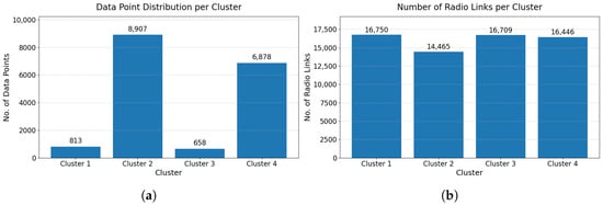
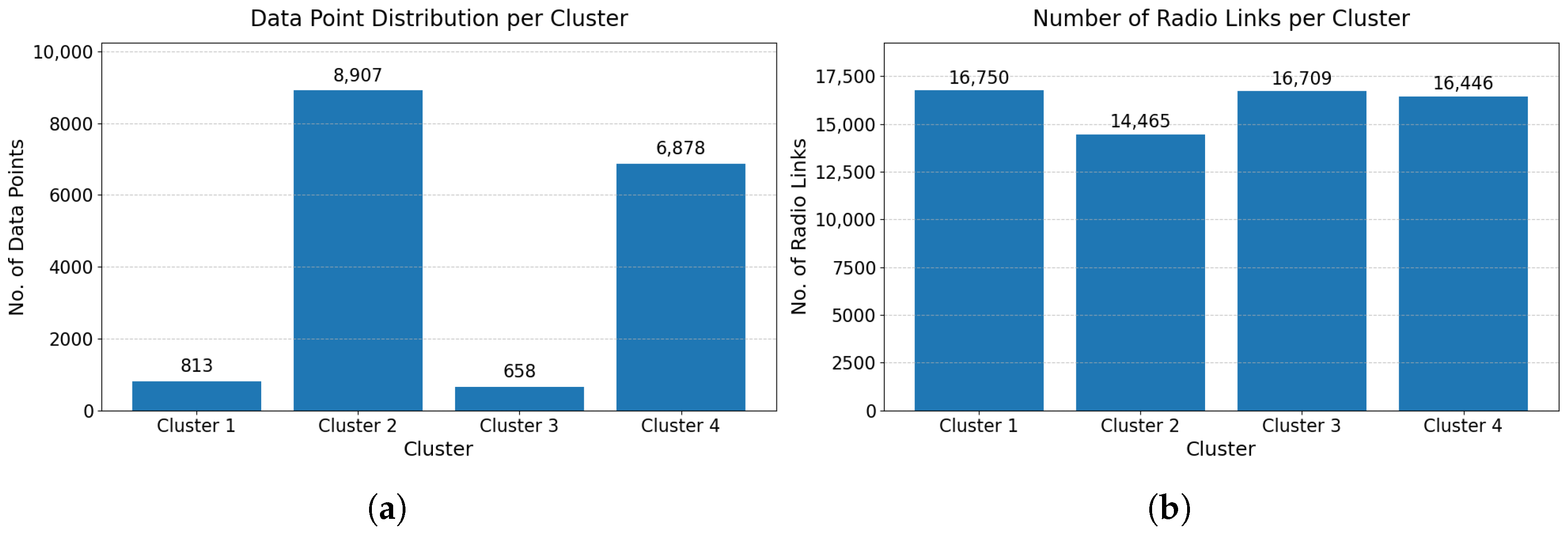
It is worth examining the distribution of data points across the clusters. As shown in Figure 16a, the number of data points was unevenly distributed among them. However, as discussed in Section 3.3.2, model calibration (i.e., the training stage) does not require data points to be located within the cluster being calibrated. As long as radio links pass through a cluster, its path loss exponent can still be estimated. Therefore, in model calibration, the distribution of data points among clusters is not the primary concern. A more important consideration is the number of radio links that pass through each cluster.

Figure 16. (a) Data point distribution per cluster and (b) number of radio links per cluster.

From the derivation in Section 3.3.2, it can be discerned that a data entry with a distance ratio $D_k=0$ indicates that the radio link for that transmission did not cross cluster k. Therefore, the number of radio links that passed through cluster k can be determined by counting all data entries with non-zero values for $D_k$. Figure 16b shows the number of radio links that passed through each cluster, indicating an almost uniform distribution.

5. Results and Discussion

5.1. Model Calibration ($\eta$ Estimation)

The dataset was split into 80% for model training and 20% for testing. Since model validation is performed per cluster, stratified sampling was used to prevent possible under-sampling of some clusters. Following the process described in Section 3.3.2, the estimates of the path loss exponents ($\eta$) for each cluster are

$$\widehat{\mathsf{\beta }}=\left[\begin{array}{c}2.109931\\ 1.460786\\ 3.636597\\ 2.612192\end{array}\right]$$

(21)

For the standard log-distance path loss model (SLDPLM), the path loss exponent was determined through the following derivation:

$$P{L}_x^{\left(i\right)}=10\eta log\left({\displaystyle \frac{d^{\left(i\right)}}{d_0}}\right)$$

(22)

Equation (22) can be rewritten as a linear regression model:

$$y^{\left(i\right)}=\theta x^{\left(i\right)}+{ϵ}^{\left(i\right)}$$

(23)

where

$$\begin{array}{cc}\hfill y^{\left(i\right)}& =P{L}_x^{\left(i\right)}\hfill \\ \hfill x^{\left(i\right)}& =log\left({\displaystyle \frac{d^{\left(i\right)}}{d_0}}\right)\hfill \\ \hfill \theta & =10\eta \hfill \end{array}$$

(24)

Minimizing the sum of squared errors, i.e., $\sum {\left({ϵ}^{\left(i\right)}\right)}^2$, gives

$$\begin{array}{cc}\hfill & {\displaystyle \frac{d}{d\theta }}\sum {\left(y^{\left(i\right)}-\theta x^{\left(i\right)}\right)}^2=0\hfill \\ \hfill & \theta \sum {\left(x^{\left(i\right)}\right)}^2=\sum x^{\left(i\right)}{y}^{\left(i\right)}\hfill \\ \hfill & \theta ={\displaystyle \frac{\sum x^{\left(i\right)}{y}^{\left(i\right)}}{\sum {\left(x^{\left(i\right)}\right)}^2}}\hfill \end{array}$$

(25)

Finally, after substituting the values for x, y, and $\theta$, the path loss exponent $\eta$ for a sample size S is given by

$$\eta ={\displaystyle \frac{{\sum }_{i=1}^{S}P{L}_x^{\left(i\right)}log\left(\frac{d^{\left(i\right)}}{d_0}\right)}{10{\sum }_{i=1}^S{\left[log\left(\frac{d^{\left(i\right)}}{d_0}\right)\right]}^2}}$$

(26)

Using Equation (26), the path loss exponent for the standard log-distance path loss model is

$$\eta =2.419453$$

(27)

5.2. Performance Evaluation

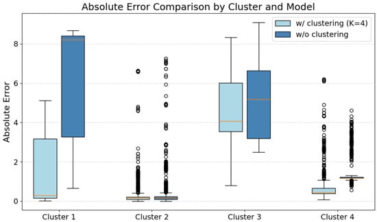
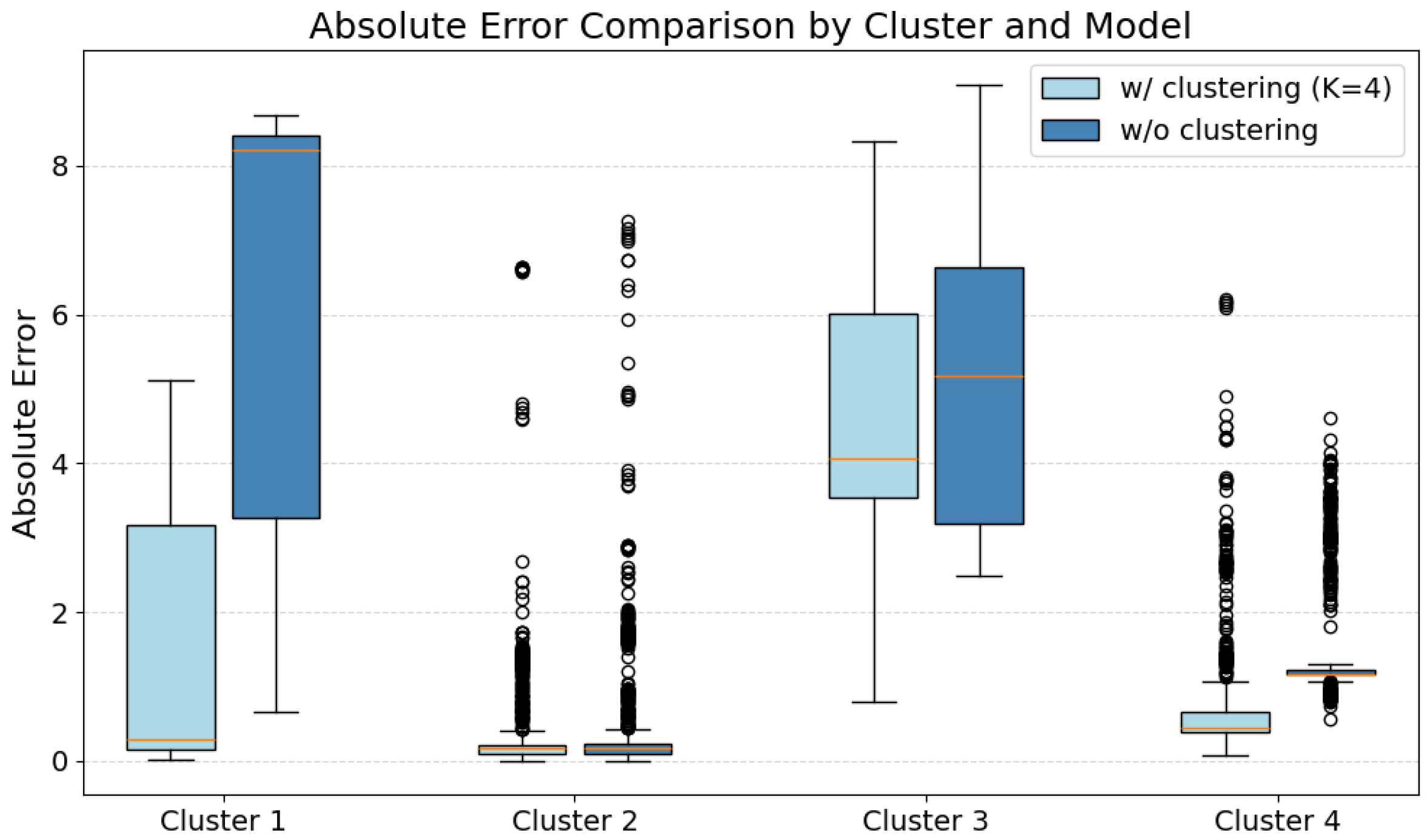
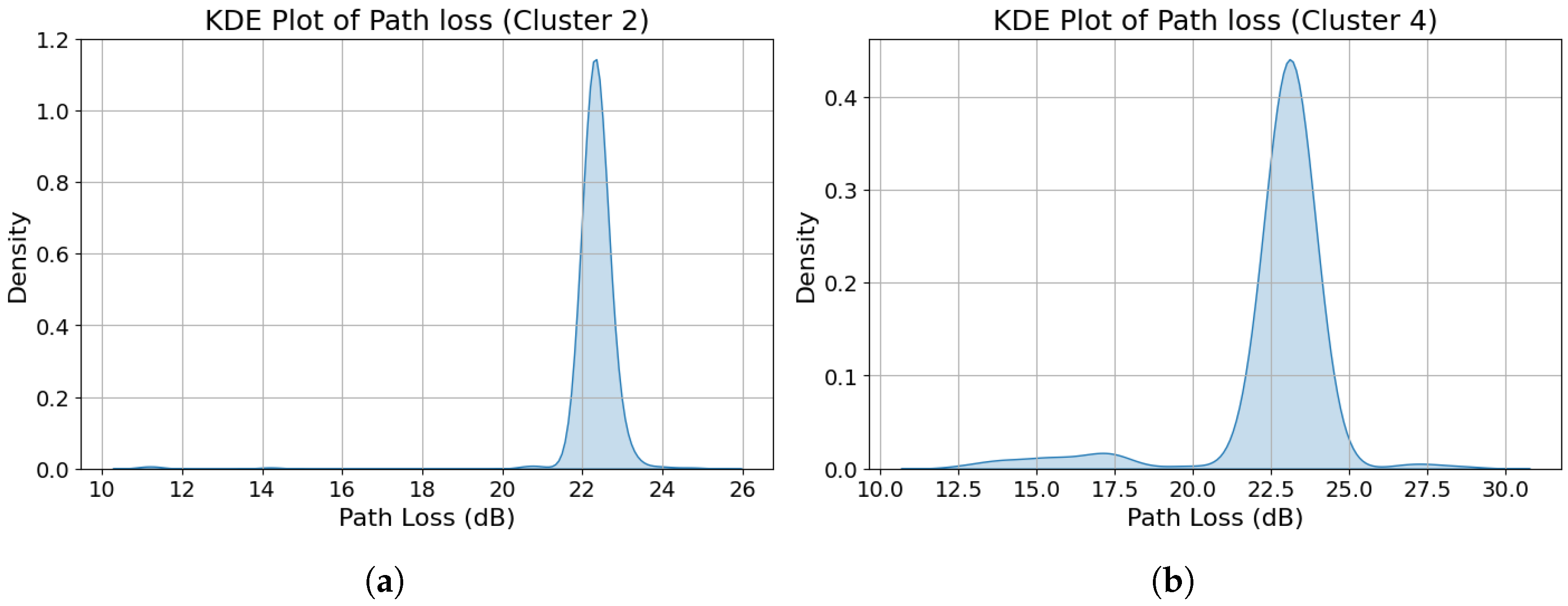
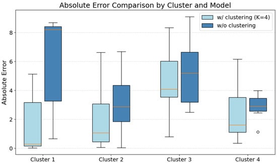
Figure 17 shows the per-cluster box plot comparison of the absolute errors of GeoSeg and the SLDPLM. The most striking feature appeared in Cluster 2 and Cluster 4, which exhibited both significant outliers and exceptionally narrow interquartile range (IQR) regions. These characteristics indicate possible underlying groupings, which is indicative of concentration of data. Specifically, the errors may have been taken from a narrow range of path loss estimate values. To further investigate, a kernel density estimation (KDE) plot of the path loss estimates was generated for these clusters to visualize the dataset concentration peaks.

Figure 17. Box plot of absolute errors for GeoSeg and standard log-distance path loss model (SLDPLM).

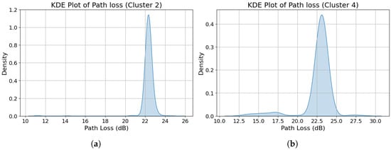
The observed data concentration in Cluster 2 and Cluster 4, evidenced by the tall, narrow peaks in their respective KDE plots (Figure 18a,b), prompted further investigation. Density-based (DBSCAN) spatial clustering was employed with parameters $ϵ=10\mathrm{m}$ and $\mathrm{minPts}=5$ to identify spatial groupings of test points in both clusters. This process revealed seven distinct groupings in Cluster 2, with one dominant group containing 84% of its test data (1496 out of 1780 points). Similarly, Cluster 4 exhibited 11 distinct groupings, with one dominant group containing 89% of its test data (1204 out of 1358 points). This spatial concentration of the data directly accounted for both the characteristic narrow peaks in the path loss KDE plots and the compact interquartile ranges (IQRs) observed in the corresponding error box plots.

Figure 18. Kernel density estimate plots of path loss values for (a) Cluster 2 and (b) Cluster 4.

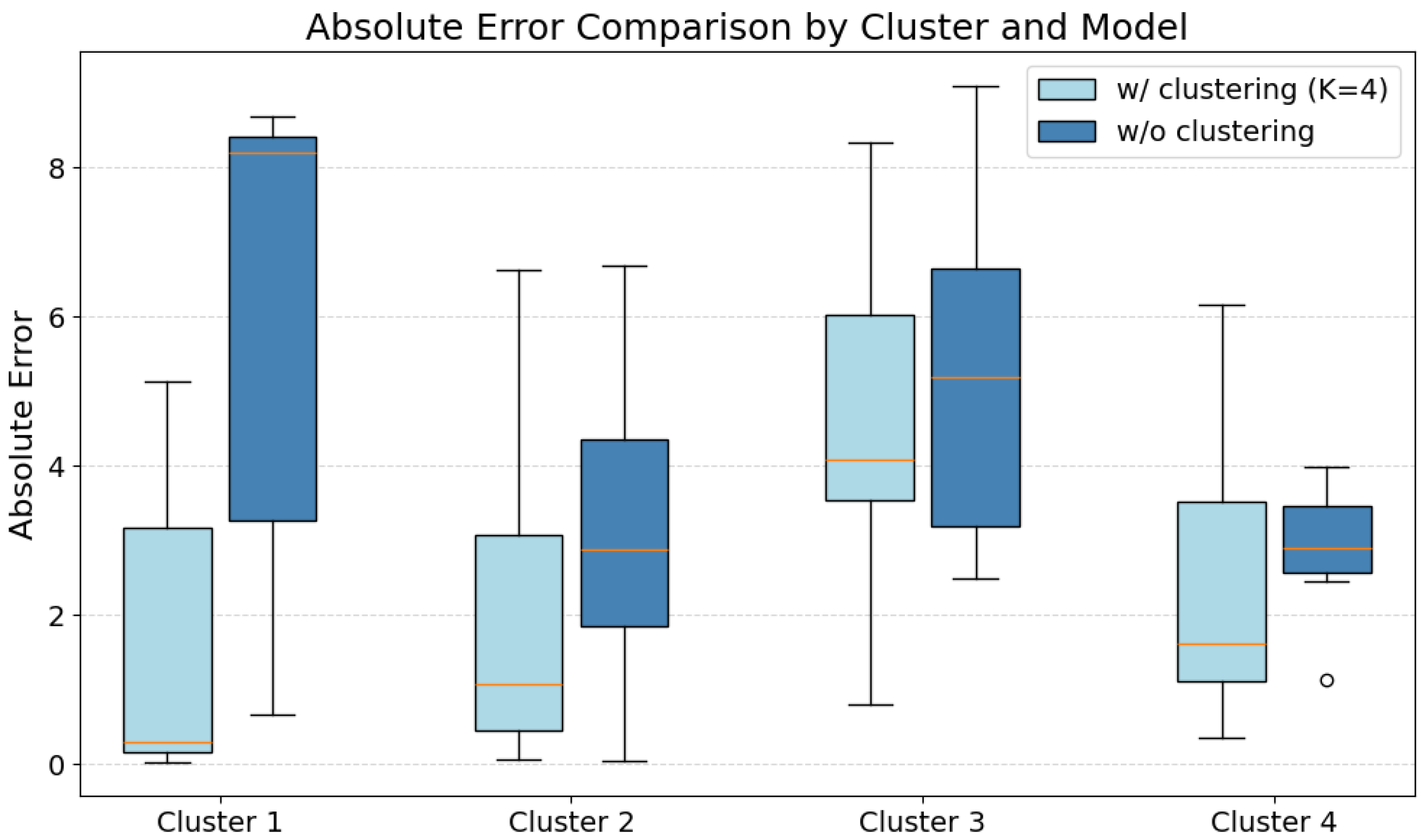
To proceed with the model performance comparison, a step was taken to mitigate the spatial bias by first averaging the path loss values within each grouping in Cluster 2 and Cluster 4 before recalculating the absolute errors. This resulted in a greatly reduced test dataset, i.e., $N_1=132$, $N_2=7$, $N_3=129$, and $N_4=11$ for Clusters 1, 2, 3, and 4, respectively. Figure 19 presents the resulting box plot after applying this correction procedure. Table 6 presents the summary statistics for GeoSeg and the standard log-distance path loss model.

Figure 19. Box plot of GeoSeg and standard log-distance path loss model for each cluster.

Table 6. Comparison of error statistics between GeoSeg and SLDPLM across clusters.

Cluster	Metric	GeoSeg	SLDPLM
1	Median Error	0.29	8.20
	Mean Error	1.54	5.94
	Std. Dev.	1.87	2.90
2	Median Error	1.08	2.87
	Mean Error	2.11	3.14
	Std. Dev.	2.34	2.04
3	Median Error	4.08	5.18
	Mean Error	4.57	5.34
	Std. Dev.	2.04	2.17
4	Median Error	1.62	2.90
	Mean Error	2.40	2.87
	Std. Dev.	1.76	0.76

In summary, the error analysis during the performance evaluation of GeoSeg highlighted the spatial distribution characteristics of the dataset. After applying the necessary data filtering, the dataset consisted of sparsely distributed measurements concentrated in dense groupings, with some groupings accounting for over 80% of all data points. These patterns became evident during the model validation phase. Aggregating the densely clustered data points drastically reduced the sample size for Clusters 2 and 4. Considering only Clusters 1 and 3, GeoSeg outperformed the standard log-distance model, with the median error dropping from 8.20 m to 0.29 m (96%) and 5.18 m to 4.08 m (21%) for Clusters 1 and 3, respectively. The disparity in the improvement magnitude suggests that the single-environment assumption, i.e., one path loss exponent $\eta$ for the entire propagation region (SLDPLM), misrepresented actual propagation conditions to varying degrees across the subregions.

6. Conclusions

This study presented GeoSeg, a segmented variant of the log-distance path loss model that combines per-link modeling and geographical clustering. Preliminary evaluation using an open-access LoRaWAN dataset showed that GeoSeg outperformed the standard log-distance path loss model, with median MAE reductions of 21% and 96% observed across the evaluated clusters. In practical terms, these improvements could support more reliable LPWAN coverage prediction, gateway placement, and localization performance in heterogeneous propagation environments.

Beyond the reported performance gains, the primary contribution of this work lies in the methodological framework used to construct GeoSeg. First, this study derived a per-link formulation of the conventional log-distance path loss model that represents a radio link as a sequence of traversed geographical subregions. This per-link formulation accounts for the anisotropic propagation behavior arising from land cover heterogeneity across different radio links. Second, since subregion identification via clustering requires a feature embedding process, this work introduced a context-aware, land cover-embedding procedure for representing propagation regions. Rather than relying on dominant land cover classes or simple land cover proportions, the proposed embedding encodes both the land cover type and its spatial position relative to the line-of-sight path, representing the propagation environment as a variable-length sequence that preserves spatial context within the radio link region. Third, this study adapted an HMM-based clustering procedure to handle large collections of variable-length sequence representations of embedded propagation regions. Taken together, these contributions establish GeoSeg as a generalized framework for integrating spatial environmental structure into LPWAN propagation modeling.

It should be noted that GeoSeg was evaluated only against the standard log-distance path loss model. Direct comparison with other per-link approaches, such as SateLoc and the per-link Okumura–Hata model, was not feasible due to differences in data requirements and missing system parameters. For example, SateLoc requires transceivers to be located within the same land cover type to estimate path loss exponents, while the per-link Okumura–Hata model requires system parameters unavailable in the dataset used in this study. Furthermore, this study relied on a single gateway from a single publicly available dataset, which limits the generalizability of the conclusions regarding GeoSeg’s effectiveness.

Future work should focus on collecting datasets with more uniform spatial coverage and complete system parameter information to enable broader comparative evaluations. In addition, measurement campaigns across geographically diverse regions and multiple gateways would also allow cross-regional validation of GeoSeg and provide deeper insights into the transferability and generalizability of the proposed framework.

References

- Singh, R.K.; Puluckul, P.P.; Berkvens, R.; Weyn, M. Energy Consumption Analysis of LPWAN Technologies and Lifetime Estimation for IoT Application. Sensors 2020, 20, 4794. [Google Scholar] [CrossRef] [Scilit] [PubMed]
- Miuccio, L.; Panno, D.; Riolo, S. A DNN-based estimate of the PRACH traffic load for massive IoT scenarios in 5G networks and beyond. Comput. Netw. 2021, 201, 108608. [Google Scholar] [CrossRef] [Scilit]
- Almuhaya, M.A.M.; Jabbar, W.A.; Sulaiman, N.; Abdulmalek, S. A Survey on LoRaWAN Technology: Recent Trends, Opportunities, Simulation Tools and Future Directions. Electronics 2022, 11, 164. [Google Scholar] [CrossRef] [Scilit]
- Sun, Z.; Yang, H.; Liu, K.; Yin, Z.; Li, Z.; Xu, W. Recent Advances in LoRa: A Comprehensive Survey. ACM Trans. Sen. Netw. 2022, 18, 1–44. [Google Scholar] [CrossRef] [Scilit]
- Jouhari, M.; Saeed, N.; Alouini, M.S.; Amhoud, E.M. A Survey on Scalable LoRaWAN for Massive IoT: Recent Advances, Potentials, and Challenges. IEEE Commun. Surv. Tutor. 2023, 25, 1841–1876. [Google Scholar] [CrossRef] [Scilit]
- The Things Industries. The Things Industries Reaches 1 Million of Connected Devices to Their LoRaWAN® Network Management Infrastructure; The Things Industries: Amsterdam, The Netherlands, 2023. [Google Scholar]
- Rademacher, M.; Linka, H.; Horstmann, T.; Henze, M. Path Loss in Urban LoRa Networks: A Large-Scale Measurement Study. In Proceedings of the 2021 IEEE 94th Vehicular Technology Conference (VTC2021-Fall); IEEE: New York, NY, USA, 2021; pp. 1–6. [Google Scholar] [CrossRef] [Scilit]
- Vo, H.; Hoang Long Nguyen, V.; Tran, V.L.; Ferrero, F.; Lee, F.Y.; Tsai, M.H. Advance Path Loss Model for Distance Estimation Using LoRaWAN Network’s Received Signal Strength Indicator (RSSI). IEEE Access 2024, 12, 83205–83216. [Google Scholar] [CrossRef] [Scilit]
- Bianco, G.M.; Giuliano, R.; Marrocco, G.; Mazzenga, F.; Mejia-Aguilar, A. LoRa System for Search and Rescue: Path-Loss Models and Procedures in Mountain Scenarios. IEEE Internet Things J. 2021, 8, 1985–1999. [Google Scholar] [CrossRef] [Scilit]
- Ballestrin, R.; Feijó, J.F.; Feldman, M.; Müller, I. Exploring Machine Learning Techniques for Path Loss Prediction in LoRa Networks. In Proceedings of the 2024 19th International Symposium on Wireless Communication Systems (ISWCS); IEEE: New York, NY, USA, 2024; pp. 1–6. [Google Scholar] [CrossRef] [Scilit]
- Onykiienko, Y.; Popovych, P.; Yaroshenko, R.; Mitsukova, A.; Beldyagina, A.; Makarenko, Y. Using RSSI Data for LoRa Network Path Loss Modeling. In Proceedings of the 2022 IEEE 41st International Conference on Electronics and Nanotechnology (ELNANO); IEEE: New York, NY, USA, 2022; pp. 576–580. [Google Scholar] [CrossRef] [Scilit]
- Demetri, S.; Zúñiga, M.; Picco, G.P.; Kuipers, F.; Bruzzone, L.; Telkamp, T. Automated estimation of link quality for LoRa: A remote sensing approach. In Proceedings of the 18th International Conference on Information Processing in Sensor Networks; Association for Computing Machinery: New York, NY, USA, 2019; pp. 145–156. [Google Scholar] [CrossRef] [Scilit]
- Lin, Y.; Dong, W.; Gao, Y.; Gu, T. Sateloc: A virtual fingerprinting approach to outdoor lora localization using satellite images. ACM Trans. Sens. Netw. (TOSN) 2021, 17, 1–28. [Google Scholar] [CrossRef] [Scilit]
- Liu, L.; Yao, Y.; Cao, Z.; Zhang, M. Deeplora: Learning accurate path loss model for long distance links in lpwan. In Proceedings of the INFOCOM, Vancouver, BC, Canada, 10–13 May 2021. [Google Scholar] [CrossRef] [Scilit]
- Aernouts, M.; Berkvens, R.; Van Vlaenderen, K.; Weyn, M. Sigfox and LoRaWAN Datasets for Fingerprint Localization in Large Urban and Rural Areas. Data 2018, 3, 13. [Google Scholar] [CrossRef] [Scilit]
- Griva, A.I.; Boursianis, A.D.; Wan, S.; Sarigiannidis, P.; Psannis, K.E.; Karagiannidis, G.; Goudos, S.K. LoRa-Based IoT Network Assessment in Rural and Urban Scenarios. Sensors 2023, 23, 1695. [Google Scholar] [CrossRef] [Scilit] [PubMed]
- Pérez, M.; Sierra-Sánchez, F.E.; Chaparro, F.; Chaves, D.M.; Paez-Rueda, C.I.; Galindo, G.P.; Fajardo, A. Coverage and Energy-Efficiency Experimental Test Performance for a Comparative Evaluation of Unlicensed LPWAN: LoRaWAN and SigFox. IEEE Access 2022, 10, 97183–97196. [Google Scholar] [CrossRef] [Scilit]
- Nagao, T.; Hayashi, T. Geographical Clustering of Path Loss Modeling for Wireless Emulation in Various Environments. In Proceedings of the 2022 16th European Conference on Antennas and Propagation (EuCAP); IEEE: New York, NY, USA, 2022; pp. 1–5. [Google Scholar] [CrossRef] [Scilit]
- Nagao, T.; Hayashi, T. Study on radio propagation prediction by machine learning using urban structure maps. In Proceedings of the 2020 14th European Conference on Antennas and Propagation (EuCAP); IEEE: New York, NY, USA, 2020; pp. 1–5. [Google Scholar] [CrossRef] [Scilit]
- Nagao, T.; Hayashi, T. A study on urban structure map extraction for radio propagation prediction using XGBoost. In Proceedings of the 2021 15th European Conference on Antennas and Propagation (EuCAP); IEEE: New York, NY, USA, 2021; pp. 1–5. [Google Scholar] [CrossRef] [Scilit]
- Duan, J.; Guo, L. Variable-Length Subsequence Clustering in Time Series. IEEE Trans. Knowl. Data Eng. 2022, 34, 983–995. [Google Scholar] [CrossRef] [Scilit]
- Khalifa, O.; Balendran, A.; Tran, V.T.; Petit, F. Clustering methods for categorical time series and sequences: A scoping review. BMC Med. Res. Methodol. 2026, 26, 123. [Google Scholar] [CrossRef] [Scilit] [PubMed]
- Abboud, A.; Backurs, A.; Williams, V.V. Quadratic-Time Hardness of LCS and other Sequence Similarity Measures. arXiv 2015, arXiv:1501.07053. [Google Scholar] [CrossRef] [Scilit]
- Salvador, S.; Chan, P. Toward accurate dynamic time warping in linear time and space. Intell. Data Anal. 2007, 11, 561–580. [Google Scholar] [CrossRef] [Scilit]
- Vlachos, M.; Kollios, G.; Gunopulos, D. Discovering similar multidimensional trajectories. In Proceedings of the 18th International Conference on Data Engineering; IEEE: New York, NY, USA, 2002; pp. 673–684. [Google Scholar] [CrossRef] [Scilit]
- Bringmann, K.; Künnemann, M. Quadratic Conditional Lower Bounds for String Problems and Dynamic Time Warping. In Proceedings of the 2015 IEEE 56th Annual Symposium on Foundations of Computer Science; IEEE: New York, NY, USA, 2015; pp. 79–97. [Google Scholar] [CrossRef] [Scilit]
- Alqahtani, A.; Ali, M.; Xie, X.; Jones, M.W. Deep Time-Series Clustering: A Review. Electronics 2021, 10, 3001. [Google Scholar] [CrossRef] [Scilit]
- Berahmand, K.; Daneshfar, F.; Salehi, E.S.; Li, Y.; Xu, Y. Autoencoders and their applications in machine learning: A survey. Artif. Intell. Rev. 2024, 57, 28. [Google Scholar] [CrossRef] [Scilit]
- Smyth, P. Clustering sequences with hidden Markov models. Adv. Neural Inf. Process. Syst. 1996, 9, 648–654. [Google Scholar]
- hmmlearn Developers. hmmlearn: Unsupervised Learning and Inference of Hidden Markov Models. Available online: https://hmmlearn.readthedocs.io/en/latest/ (accessed on 16 June 2026).
- Bhatia, L.; Breza, M.; Marfievici, R.; McCann, J.A. LoED: The LoRaWAN at the edge dataset: Dataset. In Proceedings of the Third Workshop on Data: Acquisition to Analysis (DATA’20); Association for Computing Machinery: New York, NY, USA, 2020; pp. 7–8. [Google Scholar] [CrossRef] [Scilit]
- Girolami, M.; Mavilia, F.; Berton, A.; Marrocco, G.; Bianco, G.M. An experimental dataset for search and rescue operations in avalanche scenarios based on lora technology. IEEE Access 2024, 12, 171015–171035. [Google Scholar] [CrossRef] [Scilit]
- Cardell-Oliver, R.; Hübner, C.; Leopold, M.; Beringer, J. Dataset: LoRa Underground Farm Sensor Network. In Proceedings of the 2nd Workshop on Data Acquisition to Analysis (DATA’19); Association for Computing Machinery: New York, NY, USA, 2019; pp. 26–28. [Google Scholar] [CrossRef] [Scilit]
- Arriesgado, A.; Talampas, M.C. GeoSeg: Path Loss Estimation Method for Outdoor LoRa LPWAN. In Proceedings of the 2025 International Symposium on Multimedia and Communications Technology (ISMAC); IEEE: New York, NY, USA, 2025; pp. 1–6. [Google Scholar] [CrossRef] [Scilit]
Disclaimer/Publisher’s Note: The statements, opinions and data contained in all publications are solely those of the individual author(s) and contributor(s) and not of MDPI and/or the editor(s). MDPI and/or the editor(s) disclaim responsibility for any injury to people or property resulting from any ideas, methods, instructions or products referred to in the content. |
© 2026 by the authors. Licensee MDPI, Basel, Switzerland. This article is an open access article distributed under the terms and conditions of the Creative Commons Attribution (CC BY) license.