Epidemic Dynamics Under Pulse Population Exchange

Abstract

Many epidemiological models assume either closed populations or continuous demographic turnover. We consider an intermediate setting in which exchange occurs through discrete pulses. In this paper, we introduce a population-conserving compartmental epidemiological model with pulse population exchange at a set of prescribed times. At each pulse, a fraction of the population in each compartment is replaced by a combination of susceptible and immunized individuals. In contrast to typical pulse birth or pulse vaccination models where only a single compartment undergoes a pulse population change, the pulses in this model have competing effects: removing infectious individuals reduces the force of infection, while introducing new susceptibles increases it. In addition, when some part of the incoming population is immunized, the net effect of pulses becomes state-dependent. After presenting the model, we prove both conservation of total population and non-negativity in each compartment. We then show that while the non-pulsed system has only the disease-free equilibrium, the demographic changes introduced by the pulses can produce two new types of solution: a pulse-periodic endemic equilibrium and a second wave of infection. We derive an exact expression for a post-pulse endemic equilibrium in terms of the integrals of the solutions between equispaced pulses using the Poincaré map. Next, we identify the exact threshold at which the pulse-induced reduction in the susceptible population changes sign. Above the threshold, the pulses in all compartments contribute to a net reduction in the force of infection. Below this threshold, competing effects take hold—incoming susceptible individuals replenish the susceptible compartment, while departing exposed and infectious individuals no longer contribute to secondary infections. Finally, using parameters motivated by recent outbreaks of disease on cruise ships, we characterize this threshold mechanism and investigate the effect of pulse start time on the solution trajectories.

1. Introduction

Infectious disease transmission is commonly modeled either in fully isolated populations or under assumptions of continuous demographic exchange. Many real-world systems, however, lie between these two extremes: populations remain largely closed while experiencing episodic discrete population exchange. Examples include long-duration transportation such as cross-country trains and cruise ships (pulse exchange at stations or ports), prisons and refugee camps (exchange at prescribed points in time), and worksites with seasonal workers such as farms and oil rigs. The systems studied in this paper have two key features that are sometimes overlooked by typical compartmental epidemiological SIR-type (Susceptible–Infected–Removed) frameworks. The first, and the primary mathematical novelty of this work, is that the pulse exchange acts on all compartments rather than being restricted to one or two compartments, as in pulse vaccination or pulse birth models. The second is the epidemiological assumption that the duration of infection is of the same order of magnitude as the timing between population turnover events (compared to something like airline travel where turnover would occur much faster than incubation). Although this assumption is not mathematically required, it is appropriate for the motivating applications considered here. When population turnover occurs on vastly different timescales than disease progression (for example, disease spread via airline travel), a different modeling framework would likely be more appropriate.

Systems of this type are especially vulnerable to pathogens with an asymptomatic or prodromal period, during which transmission may occur before infection is recognized. During a prodromal period, symptoms are often nonspecific, delaying recognition of infection and allowing ordinary patterns of interaction to continue. Many infections—for example, pertussis and Andes virus (ANDV)—are characterized by higher rates of viral shedding during this phase [1,2], which further stresses an already-vulnerable system. A 2026 cluster of ANDV infections aboard the Antarctic cruise ship MV Hondius [3] provides a motivating example. Though the primary transmission pathway for ANDV, and hantaviruses more generally, is through contact with aerosolized particles from rodent waste, ANDV is the only hantavirus that can be spread from person-to-person through contact with infected fluids [4,5,6]. Recurring outbreaks of measles, pertussis, varicella, influenza, and COVID-19 on cruise ships [7,8,9,10,11,12,13,14], cargo vessels [7], and cross-country rail [15] provide further motivating examples.

Though transport systems provide case studies, the system itself need not move in space. The model we present here directly generalizes to largely isolated populations with discrete turnover events. Particular real-world scenarios include congregate living environments, like prisons, which often experience a heightened incidence of infectious disease after prisoner transfer; this was a well-documented transmission pathway for early COVID-19 spread among inmates and guards [16,17,18].

In this paper, we develop a compartmental epidemiological SEAIR model (Susceptible–Exposed–Asymptomatic–Infected–Removed) for a closed population subject to pulse population exchange at prescribed times. The A component represents population in either an asymptomatic or prodromal period. In contrast to standard pulsed models in which one or two compartments undergo a sudden change (e.g., vaccination [19] or births [20,21]), we employ a “pulse population exchange” in which all compartments are affected. We allow a fraction of the population in all compartments to depart and replace that population with a mix of susceptible and immunized population. Whereas the single-compartment pulsed model acts uni-directionally on the force of infection, our model introduces competing effects of the pulses: reducing the infectious and pre-infectious populations decreases the force of infection, while backfilling with susceptible population increases it. Requiring a portion of the incoming population to be immunized introduces a state-dependence to these effects, with the directionality of the effects changing once the S and/or R populations cross particular thresholds. We show that the pulse population exchange introduces two solution types not present in the corresponding closed model: an endemic equilibrium driven by the pulses and a second peak. We then explore the threshold effects of immunization requirements for incoming population and pulse start times. The objective of this work is to develop and analyze a modeling framework for pulse population exchange rather than to calibrate the model to a specific outbreak, which would require disease-specific data, parameter estimation, sensitivity analysis, and validation against observations.

The paper is organized as follows. In Section 2 we introduce a pulsed SEAIR system of equations in which a continuous ODE system is implemented between pulses. At each pulse, a population-conserving population exchange is instantaneously applied. We prove that the coupling of the continuous and discrete systems conserves the total population and that the compartmental solutions remain non-negative for non-negative initial conditions. In Section 3, we explore the effect of the pulses on the system analytically and numerically. First, we discuss the “competing” effect of the pulses—removing an equal fraction of the population from each component both decreases the force of infection by removing infectious population and increases the force of infection by introducing new susceptible population. We present an exact analytic threshold for S which, when passed, changes the direction of the pulses for the susceptible compartment. We derive a basic reproduction number ${\mathcal{R}}_0$ for the non-pulsed system and an analytic expression for the post-pulse periodic endemic equilibrium in terms of an integral between equispaced pulses. In Section 4, we discuss the effects of parameters on the system—in particular, the threshold effects introduced by requiring a fraction of the population to be immunized and the sensitivity to the pulse start time. Section 5 concludes the paper with a discussion of the application of the model to real-world scenarios such as cruise ships and suggestions for future work.

2. The Pulsed SEAIR Model

We consider the following compartments:

• $S\left(t\right)$: susceptible population;
• $E\left(t\right)$: exposed population;
• $A\left(t\right)$: asymptomatic or prodromal population;
• $I\left(t\right)$: acute infected population;
• $R\left(t\right)$: removed population.

We assume the total population is normalized to 1 and use initial conditions $\left(S\left(0\right),E\left(0\right),A\left(0\right),I\left(0\right),R\left(0\right)\right)=\left(1-E_0,E_0,0,0,0\right)$, assuming the model begins when the first exposed population $E_0$ enters the system, unless otherwise specified. If pulses occur at $\{T_0,T_1,T_2,T_3,\dots \}$ (not necessarily equispaced), we have the following model between pulses: for $t\in (T_P,T_{P+1})$

$$\begin{array}{cc}\hfill \dot{S}& =-S\left({\beta }_{A}A+{\beta }_{I}I\right)\hfill \\ \hfill \dot{E}& =S\left({\beta }_{A}A+{\beta }_{I}I\right)-{\gamma }_{1}E\hfill \\ \hfill \dot{A}& ={\gamma }_{1}E-\left({\gamma }_2+{\gamma }_3\right)A\hfill \\ \hfill \dot{I}& ={\gamma }_{3}A-{\gamma }_{4}I\hfill \\ \hfill \dot{R}& ={\gamma }_{4}I+{\gamma }_{2}A\hfill \end{array}$$

(1)

Parameter explanations and approximate values for three example infections studied in this paper—pertussis (whooping cough), measles, and person-to-person transmitted Andes virus—are found in Table 1, with additional information about infection duration found in Table 2. Although cruise ships provide a motivating example, the parameter values reported in the tables are intended only as illustrative disease-specific benchmarks and are not representative of a particular outbreak. In applications, the parameters should be calibrated to local contact patterns, including overcrowding, treatment availability, vaccination requirements, and turnover schedules, rather than assumed to take these numerical values across all settings.

Table 1. Disease-specific parameters. All parameters are positive and approximated from infection duration data in Table 2. In the numerical experiments (Figure 1), we set ${\gamma }_2={\gamma }_3={\displaystyle \frac{1}{2}}{\gamma }^{\ast }$.

Parameter	Interpretation	Pertussis	Measles	Andes Virus
${\gamma }_1$ (days−1)	$E\to A$ transition rate, inverse of incubation period	$0.21$	$0.086$	$0.06$
$\begin{array}{c}\hfill {\gamma }^{\ast }={\gamma }_2+{\gamma }_3\end{array}$ (days−1)	$A\to \left(I\mathrm{or}R\right)$ transition rate, inverse of prodromal period	$0.11$	$0.20$	$0.32$
${\gamma }_4$ (days−1)	$I\to R$ transition rate, inverse of recovery rate	$0.51$	$0.58$	$0.33$
${\beta }_A$	infection rate from prodromal population (approximated as ${\gamma }^{\ast }{\mathcal{R}}_0$)	$1.3$	$2.6$	$0.6$
${\beta }_I$	infection rate from acutely infected population (approximated as ${\gamma }_4{\mathcal{R}}_0$)	$0.8$	$3.5$	$0.4$

Table 2. Infection stages for the three diseases fitting the infection profile studied in this paper.

Infection	Incubation Period	Prodromal Period	Acute Period	Reproduction Number ${\mathcal{R}}_0$
Pertussis	3–12 days [22,23]	1–2 weeks [2,23]	1–6 weeks [2,22]	12–17 [23,24]
Measles	10–14 days [25,26]	4–7 days [25,26]	3–4 days [25,26]	10.4–12.9 [27]
Andes virus	2–3 weeks [6,28]	2–7 days [4,5,6]	2–6 days [4,6]	1.2 [29]

Using notation consistent with the SIR literature for pulse vaccination [19] and pulse births [20,21], we employ a “pulse population exchange” when $t=T_P$ for $T_P$ in a prescribed list of times. Let $Y^{+}:=Y\left(T_P^{+}\right)$ be the population in compartment Y immediately after the pulse at time $T_P$, and $Y^{-}:=Y\left(T_P^{-}\right)$ be the population in compartment Y immediately preceding the pulse. The constant-population pulses are given by

$$\begin{array}{cc}\hfill S^{+}& =\left(1-\theta \right)S^{-}+(1-q)\theta \hfill \\ \hfill E^{+}& =(1-\theta )E^{-}\hfill \\ \hfill A^{+}& =(1-\theta )A^{-}\hfill \\ \hfill I^{+}& =\left(1-\theta \right)I^{-}\hfill \\ \hfill R^{+}& =\left(1-\theta \right)R^{-}+q\theta \hfill \end{array}$$

(2)

Parameter descriptions for the pulses can be found in Table 3. The parameter $\theta$ is the fraction of the population departing at each pulse, or the “migration factor.” By using the same $\theta$ across all compartments, we assume that the departing population is of the same composition as the internal system. This assumption is most natural in the context of the S, E, A, and R sub-populations, where symptoms are either absent, nonspecific, or mild. For the I category, having a migration factor equal to that of the other compartments is an idealization; in reality, depending on the infection and the logistics of the system, acutely infected individuals may be quarantined (migration factor and infection rate ${\beta }_I$ reduced) or medically evacuated (migration factor increased). Because quarantine of infected individuals is not the main focus of the present study, however, we keep $\theta$ the same for the I category as well. Compartmental $\theta$-values could be implemented with only minor changes to the mathematics.

Table 3. Other model parameters.

Parameter	Interpretation
$\theta \in [0,1]$	fraction departing at each pulse (migration fraction)
$q\in [0,1]$	fraction of arriving population with immunity, either through vaccination or prior exposure (immunized fraction)

As population departs, an equal amount of population (see Lemma 1) rejoins the system, this time made up only of S and R. Excluding any infected compartments in the incoming population reflects the assumption that secondary importation of infected individuals is negligible relative to the transmission within the closed continuous system. This simplification is likely reasonable for the spread of rare diseases in closed systems under pulse dynamics, as in one of our specific motivating examples of person-to-person ANDV transmission on a cruise ship [3] (see Section 1). However, to fully reflect the dynamics of a more common infection such as influenza, the model may be extended to include secondary importation of individuals in the E, A, and/or I components.

The fraction of incoming “removed” (typically immunized) population is given by q. The q parameter can be used to model an immunization requirement for entering the system or assess how the level of vaccinated population affects the outcome of epidemics [30].

We can think of the pulsed system (the continuous System 1 with pulses given in System 2) as a series of ODEs on $t\in (T_P,T_{P+1})$ with initial condition given by the post-pulse state $(S^{+},E^{+},A^{+},I^{+},R^{+})$.

Lemma 1

(Population conservation). Suppose

$$S\left(0\right)+E\left(0\right)+A\left(0\right)+I\left(0\right)+R\left(0\right)=1.$$

Then

$$S\left(t\right)+E\left(t\right)+A\left(t\right)+I\left(t\right)+R\left(t\right)=1\forall t\ge 0.$$

Proof. 

Between pulses, summing the equations in System 1 gives

$$\dot{S}+\dot{E}+\dot{A}+\dot{I}+\dot{R}=0$$

Thus, population is conserved on each interval $(T_P,T_{P+1})$. Likewise, we can see that the pulses conserve total population instantaneously at $T_P$ by summing System 2. The result is

$$S^{+}+E^{+}+A^{+}+I^{+}+R^{+}=S^{-}+E^{-}+A^{-}+I^{-}+R^{-}+\theta (1-S^{-}-E^{-}-A^{-}-I^{-}-R^{-}).$$

Since the pre-pulse state $(S^{-},E^{-},A^{-},I^{-},R^{-})$ satisfies System 1, we have $S^{-}+E^{-}+A^{-}+I^{-}+R^{-}=1$, and therefore,

$$S^{+}+E^{+}+A^{+}+I^{+}+R^{+}=S^{-}+E^{-}+A^{-}+I^{-}+R^{-}$$

i.e.,

$$\underset{t\to T_P^{+}}{\lim }S\left(t\right)+E\left(t\right)+A\left(t\right)+I\left(t\right)+R\left(t\right)=\underset{t\to T_P^{-}}{\lim }S\left(t\right)+E\left(t\right)+A\left(t\right)+I\left(t\right)+R\left(t\right)=1$$

Thus, the total population is conserved for $t\ge 0$. □

Lemma 2

(Non-negativity of solutions). Suppose

$$S\left(0\right),E\left(0\right),A\left(0\right),I\left(0\right),R\left(0\right)\ge 0.$$

Then

$$S\left(t\right),E\left(t\right),A\left(t\right),I\left(t\right),R\left(t\right)\ge 0\forall t\ge 0.$$

Proof. 

First note that the pulse operator, System 2, has non-negative coefficients $1-\theta$ and non-negative additive constants $(1-q)\theta$ and $q\theta$. Therefore, it maps non-negative pre-pulse states to non-negative post-pulse states.

Now we must check the non-negativity of solutions between pulses for $t\in (T_P,T_{P+1})$.

Given $S\left(T_P\right)\ge 0$, we can integrate the expression for $\dot{S}$ in System 1 directly, obtaining

$$S\left(t\right)=S\left(T_P\right)\exp \left(-{\int }_{T_P}^t\left({\beta }_{A}A\left(s\right)+{\beta }_{I}I\left(s\right)\right)ds\right)\ge 0$$

For the other compartments, we check the boundary.

• When $E=0$, we have $\dot{E}=S\left({\beta }_{A}A+{\beta }_{I}I\right)\ge 0$ when $A\ge 0,I\ge 0$, noting that $S\left(t\right)\ge 0$ as shown above.
• When $A=0$, we have $\dot{A}={\gamma }_{1}E\ge 0$ when $E\ge 0$.
• When $I=0$, we have $\dot{I}={\gamma }_{3}A\ge 0$ when $A\ge 0$.
• When $R=0$, we have $\dot{R}={\gamma }_{4}I+{\gamma }_{2}A\ge 0$ when $I\ge 0,A\ge 0$.

Thus, the solution can never cross the boundary of ${\mathbb{R}}_{+}^5$, so

$$S\left(t\right),E\left(t\right),A\left(t\right),I\left(t\right),R\left(t\right)\ge 0\forall t\ge 0.$$

□

Numerical Implementation

For the examples used in this paper, we solved System 1 on $(T_P,T_{P+1})$ using MATLAB R2025b’s “ode45” solver [31] with default settings. We set the initial conditions for successive intervals algebraically using System 2. All parameter sweeps were generated using a dense uniform sampling of parameters.

Since the main objective of this work is to characterize the qualitative behavior of pulse population exchange rather than fit empirical data from a specific outbreak, the disease parameters (Table 1 and Table 2) and pulse parameters (Table 3) used in the subsequent simulations are artificial approximations. Formal statistical parameter uncertainty analysis (e.g., confidence intervals, bootstrapping) is not included.

3. Effect of Pulses

It is helpful to define a quantity, often called the force of infection [19,32,33],

$$\lambda \left(t\right)=S\left(t\right)\left({\beta }_{A}A\left(t\right)+{\beta }_{I}I\left(t\right)\right)$$

(3)

A typical pulsed compartmental epidemiological model has only one or two compartments affected by a forcing term; some common frameworks are pulse vaccination [19,34,35,36] (S decreases and R increases $\Rightarrow \lambda$ decreases), pulse births [21,37] (S increases $\Rightarrow \lambda$ increases), pulse treatment or removal/quarantine [38,39] (I and/or A decreases and R increases $\Rightarrow \lambda$ decreases). In these standard models, the forcing term has a clear directional effect on the dynamics of the infection—either contributing to an increase or decrease in the force of infection.

A related category of exchange model is the so-called “metapopulation” or “patch” model, in which population movement occurs between spatially distinct populations [40,41,42]. Movement between patches may occur continuously [20,36,42,43] or at discrete pulse times [35,44]. Our model differs from conventional patch models in that it tracks a single patch coupled at pulse times to an unmodeled external population of fixed composition, with fraction $1-q$ susceptible and q immunized (removed).

In this model, the pulses have several competing outcomes that affect $\lambda$ in interesting ways. The E, A, and I compartments experience negative jumps, which decrease $\lambda$ (indirectly in the case of E because of the time delay), i.e.,

$$\begin{array}{cc}\hfill E^{+}-E^{-}& =-\theta E^{-}\hfill \\ \hfill A^{+}-A^{-}& =-\theta A^{-}\hfill \\ \hfill I^{+}-I^{-}& =-\theta I^{-}\hfill \end{array}$$

The S and R components have state-dependent jumps:

$$\begin{array}{cc}\hfill S^{+}-S^{-}& =\theta \left(1-q-S^{-}\right)\hfill \\ \hfill R^{+}-R^{-}& =\theta \left(q-R^{-}\right)\hfill \end{array}$$

In the case of $q=0$ (no immunization for incoming population),

$$\begin{array}{ccc}\hfill S^{+}-S^{-}& =\theta (1-S^{-})>0\hfill & \hfill \mathrm{for}S\in [0,1)\\ \hfill R^{+}-R^{-}& =-\theta R^{-}<0\hfill & \hfill \mathrm{for}R\in (0,1].\end{array}$$

The pulse in S contributes to an increase in the force of infection, competingwith the action of the jumps from the other components. The pulse in the R compartment has a similar mechanism. Immune population leaves the system and is directly replaced by susceptible population.

The case of $q>0$ introduces more complex behavior. The jumps for S and R change sign for $\theta \in (0,1)$ when

$$\begin{array}{cc}\hfill S^{-}& =1-q\hfill \\ \hfill R^{-}& =q\hfill \end{array}$$

In this case, q acts as a threshold parameter. Since the pulse effects are based on the pre-pulse state of the system, which includes additional E, A, and I compartments, the thresholds for S and R are not necessarily crossed simultaneously. In fact, conservation of population (Lemma 1) guarantees that these thresholds only coincide when $E=A=I=0$, i.e., at the disease-free equilibrium. To see this, recall that $S+E+A+I+R=1\forall t$, so $S+R=1-(E+A+I)$. If the thresholds are crossed simultaneously, then $(1-q)+q=1-(E+A+I)\Rightarrow E+A+I=0$. Since all solutions are non-negative by Lemma 2, this is equivalent to $E=A=I=0$. In epidemiologically meaningful scenarios, therefore, one lags the other, which creates three distinct regimes: pre-threshold, in-between thresholds, and post-threshold. In the pre-threshold regime, the pulses all contribute to a reduction in $\lambda$. When only one threshold has been crossed, one pulse (either in the S or R compartment) contributes to an increase in $\lambda$, and after both thresholds have been crossed, the pulses in both the S and the R components contribute to an increase in $\lambda$.

Assuming $S\left(0\right)\approx 1$ and $R\left(0\right)=0$, the model generally begins with $S^{-}>1-q$ and $R^{-}<q$. In this case, the S threshold is crossed first, as individuals do not reach the R component without first progressing through the E, A, and/or I categories. Once the S population decreases below $1-q$, the net effect of the pulse on the S-component switches from decreasing the susceptible population to replenishing it, contributing to an increase in the force of infection $\lambda$. Once the R population increases above its threshold at q, the net effect is the removal of the R population rather than its addition to the system. This results indirectly in an increase in the force of infection, as the population contains fewer immune individuals, so that now two pulse categories contribute to an increase in $\lambda$ rather than one. More generally, the order in which the thresholds are crossed depends on the initial conditions.

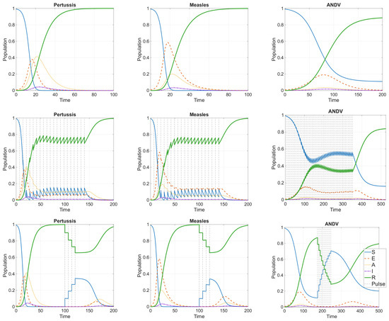
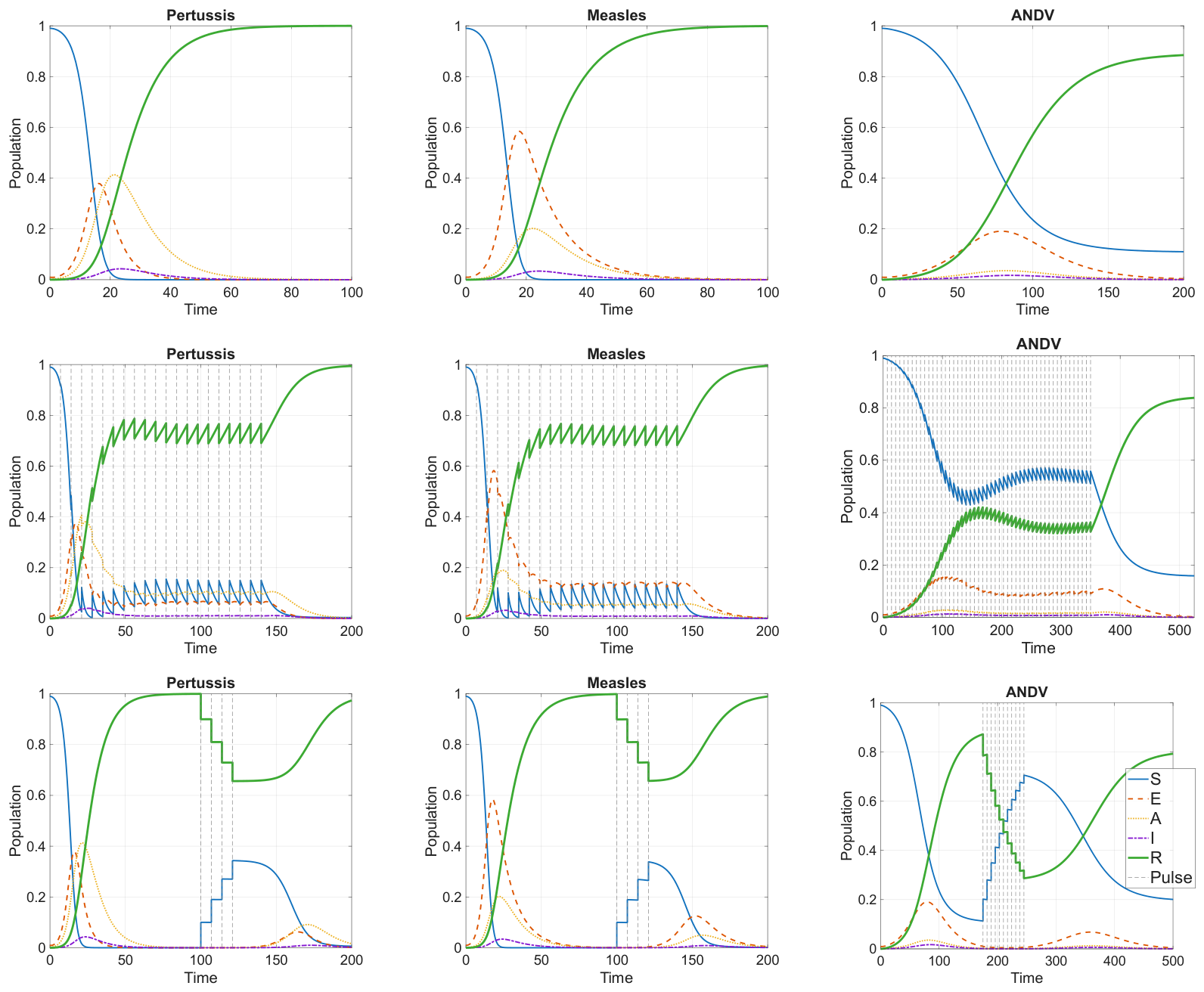
The pulses can produce two new types of behavior that are not present in the non-pulsed model: endemic equilibria in which the disease exists in the population at a low level indefinitely, and a secondary peak if pulsing is turned on after the infection has died out. Examples of each type of behavior with $q=0$ for the parameters in Table 1 are shown in Figure 1. The top row shows the system with no pulses ($\theta =0$ case), described in Section 3.1. All trajectories converge to the disease-free equilibrium. The middle row shows the system with a pulse every 7 days for 20 weeks followed by a stop in pulsing. This type of forcing can cause a periodic endemic equilibrium in which the compartment-wise population at the pulses ${\mathbf{X}}_P^{+}$ approaches a constant, as described in Section 3.2. The last row shows how starting a pulsing cycle after the infection has run its course can initiate a secondary peak by introducing newly susceptible population, as described in Section 3.3. Threshold properties for the $q>0$ case are discussed in Section 4.

Figure 1. The figure shows SEAIR curves for the three infections described in Table 1. The top row is the system with no pulses ($\theta =0$). The middle row shows the system undergoing pulses every 7 days for 20 weeks, resulting in prolonged endemic infections sustained by the pulses, which decay after pulsing stops. The bottom row shows pulses at days 100, 107, 114, and 121, resulting in a late secondary peak after the system is near its DFE. In all nine plots, we set $q=0$.

3.1. Dynamics Without Pulses

Taking $\theta =0$ removes the forcing term. The only non-negative equilibrium of the non-forced system is the disease-free equilibrium (DFE) [45]: $(S,E,A,I,R)=(S^{★},0,0,0,1-S^{★})$ for some $S^{★}\in [0,1]$. Convergence to the DFE can be seen in the top row of Figure 1. To characterize local stability of the DFE, we compute the basic reproduction number ${\mathcal{R}}_0$ using the next-generation matrix approach [46,47]. We decompose the ODE for the infected subsystem $\mathbf{Z}=(E,A,I)$ into $\dot{\mathbf{Z}}=\mathcal{F}\left(\mathbf{Z}\right)-\mathcal{V}\left(\mathbf{Z}\right)$. $\mathcal{F}$ is the vector of new infections (transmissions), which in this system consists only of the $S({\beta }_{A}A+{\beta }_{I}I)$ term. $\mathcal{V}$ is the vector of transfers into each of the compartments of $\mathbf{Z}$ (transitions).

$$\mathcal{F}\left(\mathbf{Z}\right)=\left[\begin{array}{c}S({\beta }_{A}A+{\beta }_{I}I)\\ 0\\ 0\end{array}\right],\mathcal{V}\left(\mathbf{Z}\right)=\left[\begin{array}{c}{\gamma }_{1}E\\ -{\gamma }_{1}E+({\gamma }_2+{\gamma }_3)A\\ -{\gamma }_{3}A+{\gamma }_{4}I\end{array}\right].$$

The Jacobian matrices of $\mathcal{F}\left(\mathbf{Z}\right)$ and $\mathcal{V}\left(\mathbf{Z}\right)$ evaluated at the DFE are

$$F=\left[\begin{array}{ccc}0& S^{★}{\beta }_A& S^{★}{\beta }_I\\ 0& 0& 0\\ 0& 0& 0\end{array}\right],V=\left[\begin{array}{ccc}{\gamma }_1& 0& 0\\ -{\gamma }_1& {\gamma }_2+{\gamma }_3& 0\\ 0& -{\gamma }_3& {\gamma }_4\end{array}\right]$$

Then

$$F{V}^{-1}=\left[\begin{array}{ccc}{S}^{★}\left({\displaystyle \frac{{\beta }_A}{{\gamma }_2+{\gamma }_3}}+{\displaystyle \frac{{\beta }_I{\gamma }_3}{{\gamma }_4({\gamma }_2+{\gamma }_3)}}\right)& S^{★}\left({\displaystyle \frac{{\beta }_A}{{\gamma }_2+{\gamma }_3}}+{\displaystyle \frac{{\beta }_I{\gamma }_3}{{\gamma }_4({\gamma }_2+{\gamma }_3)}}\right)& {\displaystyle \frac{S^{★}{\beta }_I}{{\gamma }_4}}\\ 0& 0& 0\\ 0& 0& 0\end{array}\right].$$

The basic reproduction number is given by the spectral radius of the next-generation matrix, which, because the matrix is upper-triangular, is

$${\mathcal{R}}_0=\left({\displaystyle \frac{{\beta }_A{\gamma }_4+{\beta }_I{\gamma }_3}{{\gamma }_4({\gamma }_2+{\gamma }_3)}}\right)S^{★}.$$

The DFE is stable if ${\mathcal{R}}_0<1$ and unstable if ${\mathcal{R}}_0>1$ [45,46,47].

3.2. Pulse-Periodic Endemic States

The middle row of Figure 1 shows trajectories that appear to converge toward a pulse-periodic endemic state. To describe this periodic fixed point for a sequence of equispaced pulses at times $\left\{T_P\right\}$, we introduce the Poincaré map [48]:

$$\begin{array}{c}\hfill {\mathbf{X}}_{P+1}^{+}=\mathsf{\Psi }\circ \mathsf{\Phi }\left({\mathbf{X}}_P^{+}\right)\end{array}$$

(4)

where $\mathsf{\Psi }$ is the pulse operator (System 2) and $\mathsf{\Phi }$ is the continuous system between pulses (System 1).

Applying the Fundamental Theorem of Calculus to the continuous system yields the integral form between pulses:

$$\begin{array}{c}\hfill \mathsf{\Phi }\left({\mathbf{X}}_P^{+}\right)={\mathbf{X}}_{P+1}^{-}={\mathbf{X}}_P^{+}+{\int }_{T_P^{+}}^{T_{P+1}^{-}}\mathbf{G}\left(\mathbf{X}\left(t\right)\right)dt\end{array}$$

where

$$\begin{array}{c}\hfill {\displaystyle \mathbf{G}\left(\mathbf{X}\left(t\right)\right)=\left[\begin{array}{c}-\lambda \left(t\right)\\ \lambda \left(t\right)-{\gamma }_{1}E\left(t\right)\\ {\gamma }_{1}E\left(t\right)-\left({\gamma }_2+{\gamma }_3\right)A\left(t\right)\\ {\gamma }_{3}A\left(t\right)-{\gamma }_{4}I\left(t\right)\\ {\gamma }_{4}I\left(t\right)+{\gamma }_{2}A\left(t\right)\end{array}\right]}\end{array}$$

with $\lambda \left(t\right)$ the force of infection given in Equation (3).

A pulse-periodic equilibrium solution is a fixed point of the Poincaré map and therefore satisfies

$$\begin{array}{c}\hfill {\mathbf{X}}_{P+1}^{+}={\mathbf{X}}_P^{+}={\mathbf{X}}^{\ast }\end{array}$$

We can find an analytic expression for the pulse-periodic equilibrium for $t=T_P$ evaluated after each pulse using ${\mathbf{X}}^{\ast }=\mathsf{\Psi }\left({\mathbf{X}}_{P+1}^{-}\right)$. For $\theta >0$,

$$\begin{array}{cc}\hfill S^{\ast }& =1-q-{\displaystyle \frac{1-\theta }{\theta }}{\int }_{T_P^{+}}^{T_{P+1}^{-}}\lambda \left(t\right)dt\hfill \\ \hfill E^{\ast }& ={\displaystyle \frac{1-\theta }{\theta }}\left[{\int }_{T_P^{+}}^{T_{P+1}^{-}}\lambda \left(t\right)dt-{\gamma }_1{\int }_{T_P^{+}}^{T_{P+1}^{-}}E\left(t\right)dt\right]\hfill \\ \hfill A^{\ast }& ={\displaystyle \frac{1-\theta }{\theta }}\left[{\gamma }_1{\int }_{T_P^{+}}^{T_{P+1}^{-}}E\left(t\right)dt-({\gamma }_2+{\gamma }_3){\int }_{T_P^{+}}^{T_{P+1}^{-}}A\left(t\right)dt\right]\hfill \\ \hfill I^{\ast }& ={\displaystyle \frac{1-\theta }{\theta }}\left[{\gamma }_3{\int }_{T_P^{+}}^{T_{P+1}^{-}}A\left(t\right)dt-{\gamma }_4{\int }_{T_P^{+}}^{T_{P+1}^{-}}I\left(t\right)dt\right]\hfill \\ \hfill R^{\ast }& =q+{\displaystyle \frac{1-\theta }{\theta }}\left[{\gamma }_4{\int }_{T_P^{+}}^{T_{P+1}^{-}}I\left(t\right)dt+{\gamma }_2{\int }_{T_P^{+}}^{T_{P+1}^{-}}A\left(t\right)dt\right]\hfill \end{array}$$

Detailed derivations may be found in Appendix A. For $\theta =0$, the pulses have no effect.

These expressions show that the pulse-periodic equilibrium is determined entirely by the cumulative compartmental flows over a single pulse interval. The pulse exchanges are simultaneously removing infectious individuals and replenishing susceptible individuals. The latter prevents the depletion of susceptibles that would otherwise terminate the epidemic.

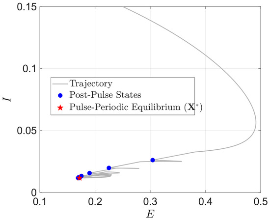
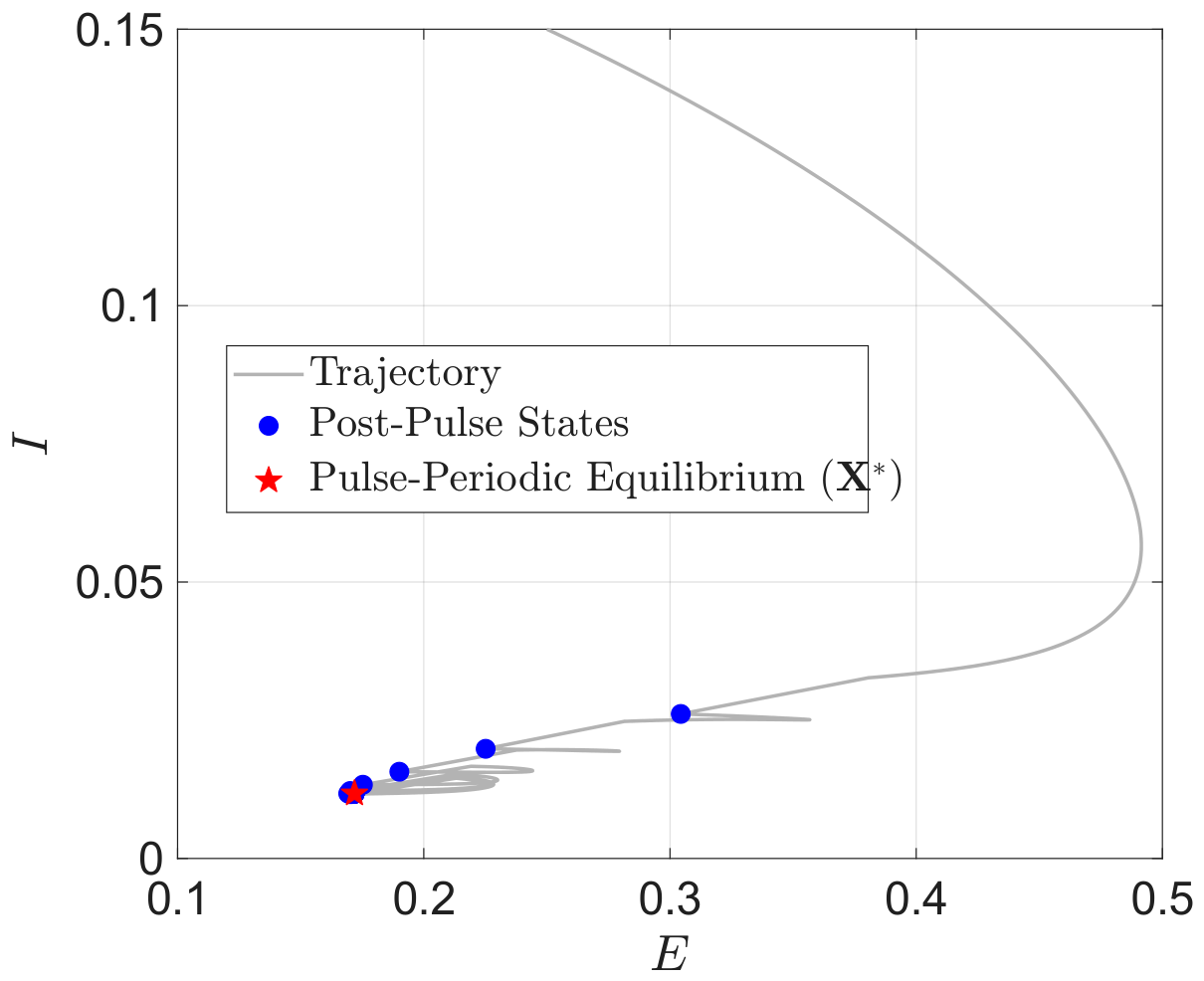
Figure 2 shows the long-term trajectory of the endemic pulsed system in terms of E and I for the measles parameters in Table 1. We use $q=0.1,\theta =0.2$, initial conditions $\left(S\right(0),E(0),A(0),I(0),R(0\left)\right)=(0.40,0.25,0.15,0.15,0.05)$, and one pulse every 7 days for 20 weeks. The system settles to an endemic equilibrium whose post-pulse fixed point is $(S^{\ast },E^{\ast },A^{\ast },I^{\ast },R^{\ast })=(0.2080,0.1718,0.0708,0.0117,0.5376)$.

Figure 2. Phase portrait in the $(E,I)$-plane illustrating convergence to a pulse-periodic endemic equilibrium.

3.3. Secondary Re-Emergence Driven by Pulses

When pulses are introduced once the system is near its DFE, the infusion of susceptible population can introduce a second wave of infection, as shown in the bottom row of Figure 1. When $q=0$, the sudden onset of pulsing increases the susceptible population and thus the force of infection.

In real life, however, population counts are discrete. The ability of an arbitrarily small residual infection to seed a future outbreak is a consequence of the continuum approximation inherent in deterministic compartmental models. In finite populations, if the infection has truly gone extinct, no secondary outbreak can occur without reintroduction of infection. Setting a compartment-specific ${\theta }_E={\theta }_A={\theta }_I=1$ for the infected components for the first pulse will “zero out” the E, A, and I compartments and prevent a second peak, maintaining the system at its DFE.

4. Immunization Requirements for Arrivals

Now we consider the case of nonzero $q\in (0,1]$. As discussed in Section 3, a nonzero q introduces a threshold effect when $S=1-q$. S begins near 1 and decreases in between pulses. If the threshold is crossed, the pulse-induced jumps in the S component change from decreasing the susceptible population to replenishing it. R begins near 0 and increases between pulses until the population crosses the $R=q$ threshold, after which the pulses act to diminish the R component and replace it with more S-population, further replenishing the susceptible compartment.

To isolate the effects of the parameter q without the time-delay effects introduced by the E and A components or the effects of different transition rates, we consider a simplified SIR model. For $t\in (T_P,T_{P+1})$,

$$\begin{array}{cc}\hfill S^{\prime }& =-\beta SI\hfill \\ \hfill I^{\prime }& =\beta SI-\gamma I\hfill \\ \hfill R^{\prime }& =\gamma I\hfill \end{array}$$

with pulses

$$\begin{array}{cc}\hfill S^{+}& =\left(1-\theta \right)S^{-}+(1-q)\theta \hfill \\ \hfill I^{+}& =\left(1-\theta \right)I^{-}\hfill \\ \hfill R^{+}& =\left(1-\theta \right)R^{-}+q\theta ,\hfill \end{array}$$

and force of infection given by

$$\begin{array}{c}\hfill {\lambda }_{SIR}\left(t\right)=\beta S\left(t\right)I\left(t\right)\end{array}$$

(5)

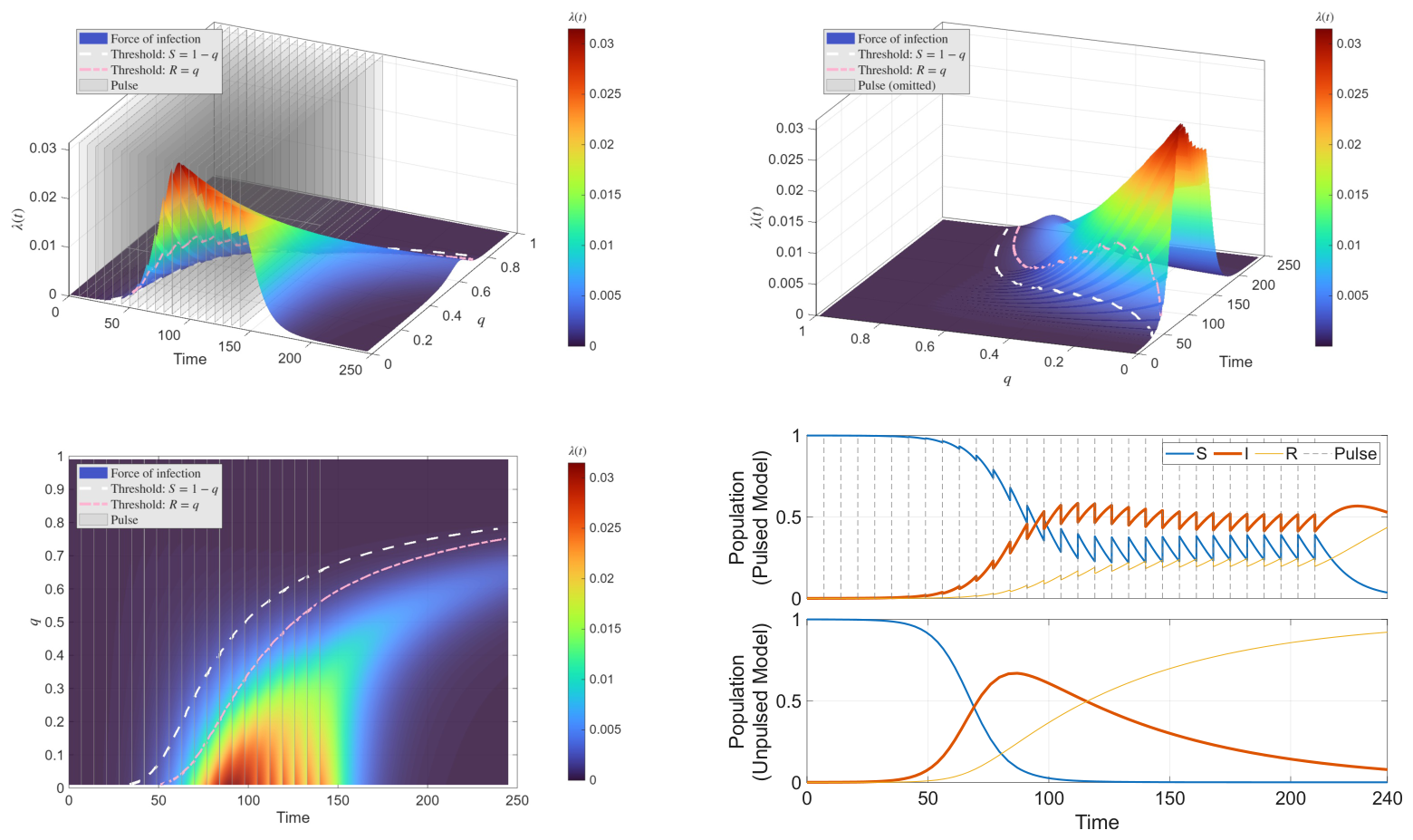
We consider an artificial infection (“Infection A”) with parameters designed to emphasize the effect of pulses. We take $\beta =0.15$, $\gamma =0.015$ (an exaggeratedly long infectious period of 66 days), $I\left(0\right)=0.0001$, and $\theta =0.2$. In this example, pulses are performed starting at $t=7$ every 7 days until $t=210$. The model stops when $t=240$. The effects of varying q are shown in Figure 3.

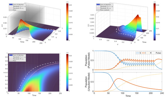
Figure 3. Force of infection ${\lambda }_{SIR}\left(t\right)$ as a function of time as q varies. The top row shows two views of the surface plot. The bottom shows a top-view heatmap of the same surface. The time at which the threshold $S=1-q$ is first met is indicated by the dotted white curve, and $R=q$ by the dotted–dashed pink curve. The bottom right shows the corresponding SIR trajectories for $q=0$, including the unpulsed system for reference.

Figure 3 shows the force of infection ${\lambda }_{SIR}\left(t\right)$ (Equation (5)) as a function of time for q varying from 0 to 1. The threshold $S=1-q$, at which the action of the pulse changes, is plotted as a dotted white line (see discussion in Section 3). The figure shows a maximum force of infection when $q=0$ near $t=75$. As q increases but before the threshold $S=1-q$ is crossed, the peak ${\lambda }_{SIR}\left(t\right)$ decreases, with the time of peak force of infection remaining about the same. For small q, the pulses replenish the susceptible population, which can lead to pulse-periodic endemic persistence.

Sensitivity to Pulse Start Time

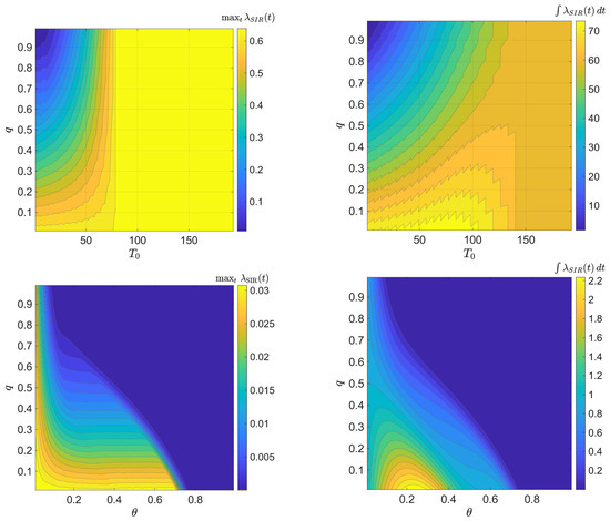
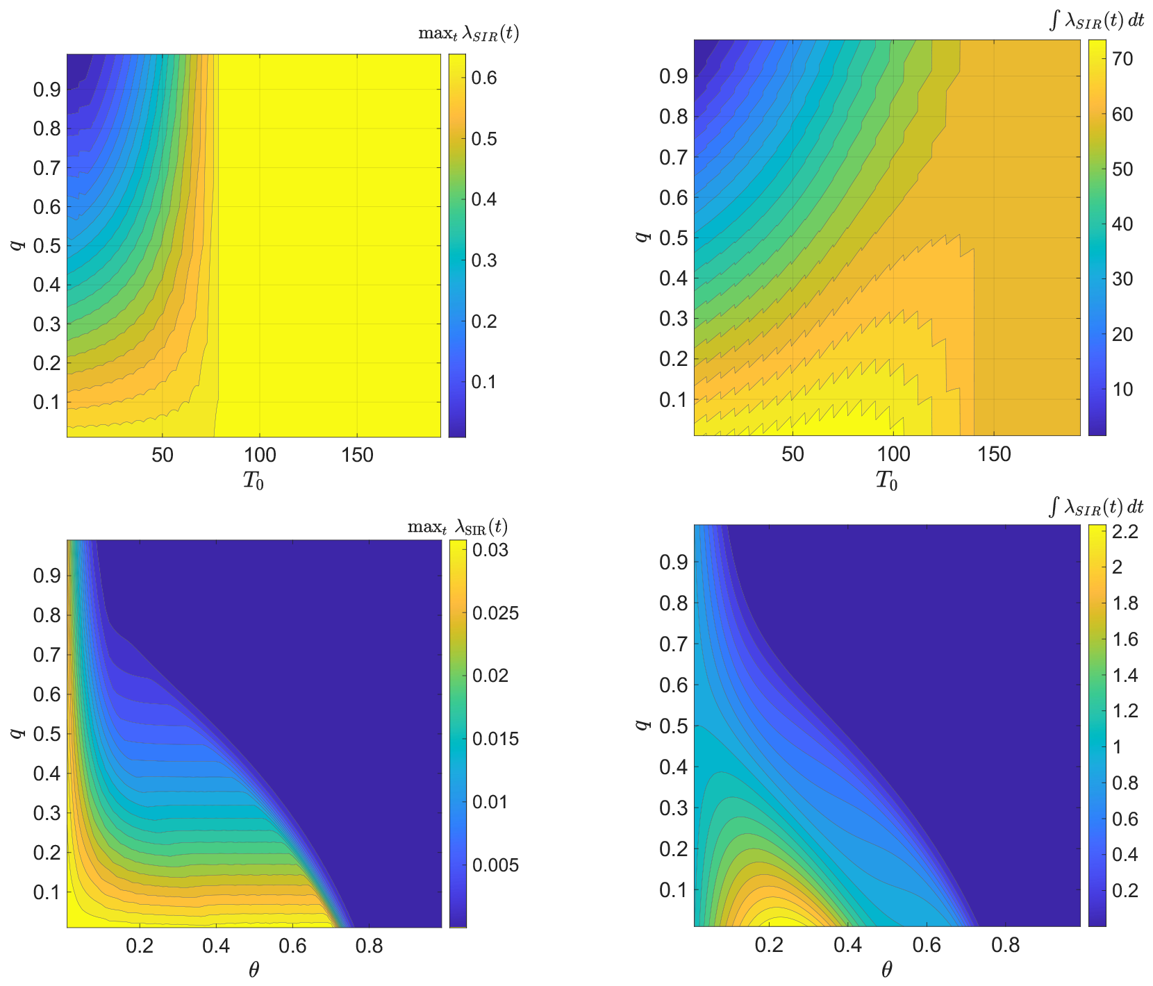
Figure 4 shows contour plots of two metrics: the peak force of infection, ${\max }_t{\lambda }_{SIR}\left(t\right)$ and the cumulative force of infection $\int {\lambda }_{SIR}\left(t\right)dt$ as q is varied with start time $T_0$ (top row) and with migration fraction $\theta$ (bottom row). The top left plot shows that the lowest peak force of infection occurs when q is near 1 and $T_0$ is near 0; the $q\approx 1$ component is expected, as nearly all incoming population is immunized, while the early $T_0$ means that infected population departs before the infection can effectively spread through the population. A late pulse start after about $t=75$ has little effect on the overall maximum force of infection. The top right plot presents the cumulative force of infection as q and $T_0$ are varied. Unlike the plot of ${\max }_t{\lambda }_{SIR}\left(t\right)$, this plot of $\int {\lambda }_{SIR}\left(t\right)dt$ is able to capture the low-level endemic solutions. This plot shows that starting the pulses between $T_0=50$ and $T_0=100$ for small q will result in high overall cumulative force of infection. Again, increasing q decreases the cumulative force of infection by introducing incoming immunized population, as long as the pulsing begins early enough. The bottom row of Figure 4 shows the combined effects of varying q and $\theta$, the departing fraction. Since $\theta$ is uniform across all compartments, small $\theta$ results in a large maximum force of infection, especially when combined with small q. The bottom right plot of the cumulative force of infection shows that when $\theta$ is too small, not enough population leaves to be backfilled with new susceptible population, even if q is near zero. A maximum cumulative force of infection occurs when $q=0$ and $\theta$ is around $0.25$.

Figure 4. Dependence of the peak force of infection (left) and cumulative force of infection (right) on the pulse parameters. The top row shows q varying with start time $T_0$, and the bottom row shows q varying with $\theta$.

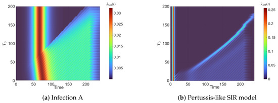
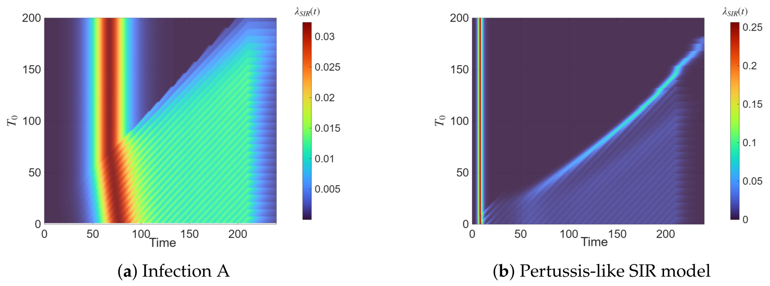
Figure 5 shows top-view heatmaps of the time progression of the force of infection ${\lambda }_{SIR}\left(t\right)$ as the pulse start time $T_0$ is varied. The figure is unchanged along the vertical axis above a jagged diagonal line, which represents the unpulsed system. The introduction of pulses shifts the time of maximum infection later, which can be most easily seen in the left panel (Figure 5a) for the artificial infection. Once the peak infection has passed, pulse-periodic endemic states persist until the pulsing is stopped. The right panel shows a pertussis-like infection using $\beta =1.3$, $\gamma =0.2$, and $I\left(0\right)=0.0001$. For this combination of parameters, the secondary peak infection can be seen as a diagonal light blue line.

Figure 5. Heatmaps of the time evolution of the force of infection ${\lambda }_{SIR}\left(t\right)$ for increasing pulse start times $T_0$ ($q=0$ case).

5. Discussion and Conclusions

5.1. Summary of Main Results

In this paper, we introduced an SEAIR model with pulse population exchange at a prescribed list of times. In contrast to standard pulsed compartmental epidemiological models where only one or two compartments are affected, an equal fraction of each compartment departs at each pulse. To maintain a constant-population model, the population is then backfilled with a combination of population from the S and R compartments. In Section 2, we proved that the population is in fact conserved, and that each compartment maintains non-negativity $\forall t\ge 0$. This population exchange introduces competing effects on the force of infection. In a closed population, the infection declines over time as the susceptible population is depleted. In this model, however, the pulses introduce additional susceptible population which can produce two new types of behavior that are not present in the non-pulsed system: an endemic trajectory in which the infection persists in the population at a low level and a secondary peak after the infection has subsided. In Section 3, we explored the effects of the pulses in several ways: first graphically and then by deriving an expression for the post-pulse periodic endemic solution in terms of the integrals between pulses. Next, in Section 4, we looked at parameter effects, including threshold effects of the immunized fraction q, and numerically demonstrated how the start time of the pulses can produce different behaviors for an artificial infection.

5.2. Application to Cruise Ships

As discussed in Section 1, this framework may be applied to many types of systems with discrete population exchange, but the assumptions of a largely closed, fully mixed population with occasional population exchange make this model particularly well-suited to describe infection dynamics on cruise ships and similar long-duration forms of transportation (e.g., trains and cargo vessels). The spread of infectious disease in mobile populations is often modeled using PDEs [32,49], but this ODE framework may provide an appropriate level of abstraction when the spatial component is not a driving factor in the spread.

Cruise ships often experience repeated outbreaks of infectious disease. There are likely many contributing factors: a large population in close quarters for an extended duration [9,50], crew members from countries without organized vaccination programs [8,50], passengers with a higher than average median age and additional risk factors [7,9,50], and shore-acquired infections [9,51]. The present model suggests an additional mechanism; repeated passenger exchange continually replenishes the susceptible population, interrupting the depletion of susceptibles that would otherwise cause the infection to die out. Whether the presence of an endemic low-level infection represents some actual disease process on cruise ships or related systems is an open problem at this time that would require model calibration and extensive data collection.

Our results suggest that requiring boarding passengers to be immunized (where possible) can be an effective strategy for mitigating this prolonged infectious state. If no immunization is possible (e.g., the $q=0$ case), temporary quarantine (delaying passenger exchange by increasing $T_0$) may be an effective measure to limit the cumulative force of infection, but results in an earlier peak in this model, as no infectious population leaves the system, and may also result in a later secondary peak.

5.3. Future Work

In this study, the only source of infection was an initial exposed population. As mentioned in Section 3, this reflects an assumption that any importation of infection is negligible compared to the infections generated within the system. This assumption makes the most sense in the case of rare diseases such as person-to-person ANDV transmission [3]. However, shore-acquired infection (at ports of call) is a common mode of disease spread on cruise ships [9]. Therefore, a reasonable future extension would be to allow the arriving population to include infectious or pre-infectious categories E, A, or I. This would naturally require more parameters analogous to our immunized fraction q—an exposed fraction, an asymptomatic fraction, and an infectious fraction. A pulse map for such a system is

$$\begin{array}{cc}\hfill S^{+}& =\left(1-\theta \right)S^{-}+(1-\left[q_E+q_A+q_I+q_R\right])\theta \hfill \\ \hfill E^{+}& =(1-\theta )E^{-}+q_E\theta \hfill \\ \hfill A^{+}& =(1-\theta )A^{-}+q_A\theta \hfill \\ \hfill I^{+}& =\left(1-\theta \right)I^{-}+q_I\theta \hfill \\ \hfill R^{+}& =\left(1-\theta \right)R^{-}+q_R\theta \hfill \end{array}$$

with $0\le q_E+q_A+q_I+q_R\le 1$.

As with many other ODE-based SIR-type systems, we assume a “well-mixed” population, which means that our model does not capture heterogeneous contact patterns. In situations where contact structure is a primary driver of infection spread, an agent-based model [52,53] or social network model [54] may be more appropriate. Adding stratification to account for differences in subpopulations—on a cruise ship these might be crew members and passengers [7,9], or passengers stratified by age [7] or deck [55]—would also make the model more realistic, as each group may have different vulnerabilities, vaccination statuses, and behavior [7,9].

The model introduced here may serve as a starting point for a more complex network-based model, with coupled metapopulations exchanging population at pulses. Previously, network-based metapopulation exchange models have been studied with pulse migration [36,44], often incorporating other pulsed mechanisms like births [20] or vaccinations [36]. Adding stochastic effects into the model—for example in the migration fraction $\theta$ or the immunized fraction q—is also a promising extension and may make the model more realistic [43]. The pulse times or exchange fractions could also be treated as state-dependent control variables, for example, in response to current infection levels; the control problem may be more complex than expected, as decreasing pulse frequency or delaying the first pulse reduces susceptible replenishment but also decreases the removal of infectious population. A delayed exchange event may also increase the possibility of a secondary peak, as illustrated in the bottom row of Figure 1 and Figure 5b.

In a network-based metapopulation model, we can also study the dual problem by tracking the departed E, A, and I population at each vertex to assess the epidemiological impact of, for example, cruise ships on their ports of call. The result would be a type of percolation centrality study [56,57] in which the impact of network topology and system parameters would determine the most affected vertices. This type of study would help identify, for example, ports of call experiencing the highest burden of infectious disease from a cruise line [58]. Examining how network topology, inter-population exchange, and other topologically defined parameters affect the dynamics of the system is another promising direction which can build on our previous work on PDE-based network models [32,56,59]. A rigorous mathematical analysis of the pulse-periodic solutions, including conditions for their existence, uniqueness, and stability, remains an important direction for future work.

References

- Ferrés, M.; Martínez-Valdebenito, C.; Henriquez, C.; Marco, C.; Angulo, J.; Barrera, A.; Palma, C.; Pinto, G.B.; Cuiza, A.; Ferreira, L.; et al. Viral shedding and viraemia of Andes virus during acute hantavirus infection: A prospective study. Lancet Infect. Dis. 2024, 24, 775–782. [Google Scholar] [CrossRef] [Scilit] [PubMed]
- Kline, J.M.; Smith, E.A.; Zavala, A. Pertussis: Common questions and answers. Am. Fam. Physician 2021, 104, 186–192. [Google Scholar] [PubMed]
- Velavan, T.P.; Schmidt-Chanasit, J. When rare zoonoses travel: Andes virus, hantavirus cardiopulmonary syndrome, and the preparedness gap. Int. J. Infect. Dis. 2026, 169, 108778. [Google Scholar] [CrossRef] [Scilit] [PubMed]
- Singh, S.; Numan, A.; Sharma, D.; Shukla, R.; Alexander, A.; Jain, G.K.; Ahmad, F.J.; Kesharwani, P. Epidemiology, virology and clinical aspects of hantavirus infections: An overview. Int. J. Environ. Health Res. 2022, 32, 1815–1826. [Google Scholar] [CrossRef] [Scilit] [PubMed]
- Martinez, V.P.; Bellomo, C.; San Juan, J.; Pinna, D.; Forlenza, R.; Elder, M.; Padula, P.J. Person-to-person transmission of Andes virus. Emerg. Infect. Dis. 2005, 11, 1848. [Google Scholar] [CrossRef] [Scilit] [PubMed]
- Vial, P.A.; Ferrés, M.; Vial, C.; Klingström, J.; Ahlm, C.; López, R.; Le Corre, N.; Mertz, G.J. Hantavirus in humans: A review of clinical aspects and management. Lancet Infect. Dis. 2023, 23, e371–e382. [Google Scholar] [CrossRef] [Scilit] [PubMed]
- Regan, J.J.; Vega, J.S.; Brown, C.M. Infectious illnesses on cruise and cargo ships. In Infectious Diseases; John Wiley & Sons, Ltd.: Hoboken, NJ, USA, 2017; Volume 4, pp. 35–44. [Google Scholar] [CrossRef] [Scilit]
- Rice, M.E.; Bannerman, M.; Marin, M.; Lopez, A.S.; Lewis, M.M.; Stamatakis, C.E.; Regan, J.J. Maritime varicella illness and death reporting, US, 2010–2015. Travel Med. Infect. Dis. 2018, 23, 27–33. [Google Scholar] [CrossRef] [Scilit] [PubMed]
- Kak, V. Infections on cruise ships. Microbiol. Spectr. 2015, 3, 10–1128. [Google Scholar] [CrossRef] [Scilit] [PubMed]
- Brotherton, J.; Delpech, V.; Gilbert, G.; Hatzi, S.; Paraskevopoulos, P.; McAnulty, J. A large outbreak of influenza A and B on a cruise ship causing widespread morbidity. Epidemiol. Infect. 2003, 130, 263–271. [Google Scholar] [CrossRef] [Scilit] [PubMed]
- Millman, A.J.; Kornylo Duong, K.; Lafond, K.; Green, N.M.; Lippold, S.A.; Jhung, M.A. Influenza outbreaks among passengers and crew on two cruise ships: A recent account of preparedness and response to an ever-present challenge. J. Travel Med. 2015, 22, 306–311. [Google Scholar] [CrossRef] [Scilit] [PubMed][Green Version]
- Ward, K.A.; Armstrong, P.; McAnulty, J.M.; Iwasenko, J.M.; Dwyer, D.E. Outbreaks of pandemic (H1N1) 2009 and seasonal influenza A (H3N2) on cruise ship. Emerg. Infect. Dis. 2010, 16, 1731–1737. [Google Scholar] [CrossRef] [Scilit] [PubMed]
- Filia, A.; Bella, A.; Cadeddu, G.; Milia, M.R.; Del Manso, M.; Rota, M.C.; Magurano, F.; Nicoletti, L.; Declich, S. Extensive nosocomial transmission of measles originating in cruise ship passenger, Sardinia, Italy, 2014. Emerg. Infect. Dis. 2015, 21, 1444–1446. [Google Scholar] [CrossRef] [Scilit] [PubMed]
- Bert, F.; Scaioli, G.; Gualano, M.R.; Passi, S.; Specchia, M.L.; Cadeddu, C.; Viglianchino, C.; Siliquini, R. Norovirus outbreaks on commercial cruise ships: A systematic review and new targets for the public health agenda. Food Environ. Virol. 2014, 6, 67–74. [Google Scholar] [CrossRef] [Scilit] [PubMed]
- Kim, H.; Schultz-Heienbrok, R.; Uhle, M.; Neubert, J.; Ball, F.; Metz, M.; Gravert, C. Longitudinal study of SARS-CoV-2 infections in different employee groups of long distance train services from June 2020 until February 2021 in Germany. Epidemiol. Infect. 2022, 150, 1–22. [Google Scholar] [CrossRef] [Scilit] [PubMed]
- Parsons, T.L.; Worden, L. Assessing the risk of cascading COVID-19 outbreaks from prison-to-prison transfers. Epidemics 2021, 37, 100532. [Google Scholar] [CrossRef] [Scilit] [PubMed]
- Beaudry, G.; Zhong, S.; Whiting, D.; Javid, B.; Frater, J.; Fazel, S. Managing outbreaks of highly contagious diseases in prisons: A systematic review. BMJ Glob. Health 2020, 5, e003201. [Google Scholar] [CrossRef] [Scilit] [PubMed]
- Jenness, S.M.; Wallrafen-Sam, K.; Schneider, I.; Kennedy, S.; Akiyama, M.J.; Spaulding, A.C. Dynamic contact networks of residents of an urban jail in the era of SARS-CoV-2. Epidemics 2024, 47, 100772. [Google Scholar] [CrossRef] [Scilit] [PubMed]
- Gao, S.; Teng, Z.; Nieto, J.J.; Torres, A. Analysis of an SIR epidemic model with pulse vaccination and distributed time delay. BioMed Res. Int. 2007, 2007, 064870. [Google Scholar] [CrossRef] [Scilit] [PubMed]
- Colombi, D.; Serra-Cobo, J.; Métras, R.; Apolloni, A.; Poletto, C.; López-Roig, M.; Bourhy, H.; Colizza, V. Mechanisms for lyssavirus persistence in non-synanthropic bats in Europe: Insights from a modeling study. Sci. Rep. 2019, 9, 537. [Google Scholar] [CrossRef] [Scilit] [PubMed]
- Clayton, T.; Duke-Sylvester, S.; Gross, L.J.; Lenhart, S.; Real, L.A. Optimal control of a rabies epidemic model with a birth pulse. J. Biol. Dyn. 2010, 4, 43–58. [Google Scholar] [CrossRef] [Scilit] [PubMed]
- Chhatwal, J.; Reid, D.; Pinkerton, I.W. Infectious Diseases. In Hutchison’s Atlas of Paediatric Physical Diagnosis, 1st ed.; Goel, K.M., Carachi, R., Cass, H., Eds.; Jaypee Brothers Medical Publishers: New Delhi, India, 2014. [Google Scholar]
- Nieves, D.J.; Heininger, U. Bordetella pertussis. Microbiol. Spectr. 2016, 4, 10–1128. [Google Scholar] [CrossRef] [Scilit] [PubMed]
- Belcher, T.; Dubois, V.; Rivera-Millot, A.; Locht, C.; Jacob-Dubuisson, F. Pathogenicity and virulence of Bordetella pertussis and its adaptation to its strictly human host. Virulence 2021, 12, 2608–2632. [Google Scholar] [CrossRef] [Scilit] [PubMed]
- World Health Organization. Measles Fact Sheet, 2025. Available online: https://www.who.int/news-room/fact-sheets/detail/measles (accessed on 18 May 2026).
- Xavier, A.R.; Rodrigues, T.S.; Santos, L.S.; Lacerda, G.S.; Kanaan, S. Clinical, laboratorial diagnosis and prophylaxis of measles in Brazil. J. Bras. De Patol. E Med. Lab. 2019, 55, 390–401. [Google Scholar] [CrossRef] [Scilit]
- Guerra, F.M.; Bolotin, S.; Lim, G.; Heffernan, J.; Deeks, S.L.; Li, Y.; Crowcroft, N.S. The basic reproduction number (R0) of measles: A systematic review. Lancet Infect. Dis. 2017, 17, e420–e428. [Google Scholar] [CrossRef] [Scilit] [PubMed]
- Riquelme, R.; Rioseco, M.L.; Bastidas, L.; Trincado, D.; Riquelme, M.; Loyola, H.; Valdivieso, F. Hantavirus pulmonary syndrome, southern Chile, 1995–2012. Emerg. Infect. Dis. 2015, 21, 562. [Google Scholar] [CrossRef] [Scilit] [PubMed]
- Martínez, V.P.; Di Paola, N.; Alonso, D.O.; Pérez-Sautu, U.; Bellomo, C.M.; Iglesias, A.A.; Coelho, R.M.; López, B.; Periolo, N.; Larson, P.A.; et al. Super-spreaders’ and person-to-person transmission of Andes virus in Argentina. N. Engl. J. Med. 2020, 383, 2230–2241. [Google Scholar] [CrossRef] [Scilit] [PubMed]
- Mouchtouri, V.A.; Lewis, H.C.; Hadjichristodoulou, C.; Partnership, E.S.A.J.A. A systematic review for vaccine-preventable diseases on ships: Evidence for cross-border transmission and for pre-employment immunization need. Int. J. Environ. Res. Public Health 2019, 16, 2713. [Google Scholar] [CrossRef] [Scilit] [PubMed]
- The MathWorks, Inc. MATLAB R2025b, Natick, MA, USA, 2025. Available online: https://www.mathworks.com/ (accessed on 13 July 2026).
- Kravitz, H.; Durón, C.; Nieves, B.; Brio, M. Data-driven optimization and parameter estimation for a metric graph epidemic model with applications to COVID-19 spread in Poland: A real-world example of optimization for a challenging Rosenbrock-type objective function. An. Int. J. Optim. Control Theor. Appl. (IJOCTA) 2025, 15. [Google Scholar] [CrossRef] [Scilit]
- Oke, M.; Ogunmiloro, O.; Akinwumi, C.; Raji, R. Mathematical modeling and stability analysis of a SIRV epidemic model with non-linear force of infection and treatment. Commun. Math. Appl. 2019, 10, 717. [Google Scholar] [CrossRef] [Scilit]
- Meng, X.; Li, Z.; Wang, X. Dynamics of a novel nonlinear SIR model with double epidemic hypothesis and impulsive effects. Nonlinear Dyn. 2010, 59, 503–513. [Google Scholar] [CrossRef] [Scilit] [PubMed]
- Jiao, J.; Cai, S.; Li, L. Impulsive vaccination and dispersal on dynamics of an SIR epidemic model with restricting infected individuals boarding transports. Phys. A Stat. Mech. Its Appl. 2016, 449, 145–159. [Google Scholar] [CrossRef] [Scilit] [PubMed]
- Terry, A.J. Pulse vaccination strategies in a metapopulation SIR model. Math. Biosci. Eng. 2010, 7, 455–477. [Google Scholar] [CrossRef] [Scilit] [PubMed]
- Peel, A.J.; Pulliam, J.; Luis, A.; Plowright, R.; O’Shea, T.; Hayman, D.; Wood, J.L.; Webb, C.; Restif, O. The effect of seasonal birth pulses on pathogen persistence in wild mammal populations. Proc. R. Soc. B Biol. Sci. 2014, 281, 20132962. [Google Scholar] [CrossRef] [Scilit] [PubMed]
- Bolzoni, L.; Tessoni, V.; Groppi, M.; De Leo, G.A. React or wait: Which optimal culling strategy to control infectious diseases in wildlife. J. Math. Biol. 2014, 69, 1001–1025. [Google Scholar] [CrossRef] [Scilit] [PubMed]
- Tang, S.; Xiao, Y.; Clancy, D. New modelling approach concerning integrated disease control and cost-effectivity. Nonlinear Anal. Theory Methods Appl. 2005, 63, 439–471. [Google Scholar] [CrossRef] [Scilit]
- Sattenspiel, L.; Herring, D.A. Simulating the effect of quarantine on the spread of the 1918–19 flu in central Canada. Bull. Math. Biol. 2003, 65, 1–26. [Google Scholar] [CrossRef] [Scilit] [PubMed]
- van den Driessche, P. Spatial Structure: Patch Models. In Mathematical Epidemiology; Brauer, F., van den Driessche, P., Wu, J., Eds.; Springer: Berlin/Heidelberg, Germany, 2008; pp. 179–189. [Google Scholar] [CrossRef] [Scilit]
- Chen, S.; Owolabi, Y.; Li, A.; Lo, E.; Robinson, P.; Janies, D.; Lee, C.; Dulin, M. Patch dynamics modeling framework from pathogens’ perspective: Unified and standardized approach for complicated epidemic systems. PLoS ONE 2020, 15, e0238186. [Google Scholar] [CrossRef] [Scilit] [PubMed]
- Shah, S.M.A.; Gang, P.; Alkhazzan, A. Stochastic Modeling and Analysis of Hepatitis B Virus Dynamics Under Transportation and Lévy Noise. J. Appl. Math. 2026, 2026, 9297530. [Google Scholar] [CrossRef] [Scilit]
- Simoy, M.I.; Simoy, M.V.; Canziani, G.A. Epidemic metapopulation model on weighted directed networks with pulse movements between nodes. Int. J. Appl. Comput. Math. 2022, 8, 39. [Google Scholar] [CrossRef] [Scilit]
- Keeling, M.J.; Rohani, P. Modeling Infectious Diseases in Humans and Animals; Princeton University Press: Princeton, NJ, USA, 2008. [Google Scholar] [CrossRef] [Scilit]
- Diekmann, O.; Heesterbeek, J.A.P.; Roberts, M.G. The construction of next-generation matrices for compartmental epidemic models. J. R. Soc. Interface 2009, 7, 873. [Google Scholar] [CrossRef] [Scilit] [PubMed]
- Van den Driessche, P.; Watmough, J. Reproduction numbers and sub-threshold endemic equilibria for compartmental models of disease transmission. Math. Biosci. 2002, 180, 29–48. [Google Scholar] [CrossRef] [Scilit] [PubMed]
- Strogatz, S.H. Nonlinear Dynamics and Chaos: With Applications to Physics, Biology, Chemistry, and Engineering, 2nd ed.; CRC Press: Boca Raton, FL, USA, 2015. [Google Scholar] [CrossRef] [Scilit]
- Besse, C.; Faye, G. Dynamics of epidemic spreading on connected graphs. J. Math. Biol. 2021, 82, 52. [Google Scholar] [CrossRef] [Scilit] [PubMed]
- McCarter, Y.S. Infectious disease outbreaks on cruise ships. Clin. Microbiol. Newsl. 2009, 31, 161–168. [Google Scholar] [CrossRef] [Scilit]
- De Bellis, A.; Bizzotto, A.; Anagnostopoulos, L.; Kourentis, L.; Marziano, V.; Mouchtouri, V.; Merler, S.; Guzzetta, G. Mitigating norovirus spread on cruise ships: A model-based assessment of diagnostic timing and isolation. J. Travel Med. 2025, 32, taaf059. [Google Scholar] [CrossRef] [Scilit] [PubMed]
- Hackl, J.; Dubernet, T. Epidemic spreading in urban areas using agent-based transportation models. Future Internet 2019, 11, 92. [Google Scholar] [CrossRef] [Scilit]
- Borjigin, S.G.; He, Q.; Niemeier, D.A. COVID-19 transmission in US transit buses: A scenario-based approach with agent-based simulation modeling (ABSM). Commun. Transp. Res. 2023, 3, 100090. [Google Scholar] [CrossRef] [Scilit]
- Liu, F.; Li, X.; Zhu, G. Using the contact network model and Metropolis-Hastings sampling to reconstruct the COVID-19 spread on the “Diamond Princess”. Sci. Bull. 2020, 65, 1297–1305. [Google Scholar] [CrossRef] [Scilit] [PubMed]
- Lai, C.C.; Hsu, C.Y.; Jen, H.H.; Yen, A.M.F.; Chan, C.C.; Chen, H.H. The Bayesian Susceptible-Exposed-Infected-Recovered model for the outbreak of COVID-19 on the Diamond Princess Cruise Ship. Stoch. Environ. Res. Risk Assess. 2021, 35, 1319–1333. [Google Scholar] [CrossRef] [Scilit] [PubMed]
- Durón, C.; Kravitz, H.; Brio, M. Edge percolation centrality: A new measure to quantify the influence of edges during percolation in networks. PLoS ONE 2025, 20, e0331475. [Google Scholar] [CrossRef] [Scilit] [PubMed]
- Piraveenan, M.; Prokopenko, M.; Hossain, L. Percolation centrality: Quantifying graph-theoretic impact of nodes during percolation in networks. PLoS ONE 2013, 8, e53095. [Google Scholar] [CrossRef] [Scilit] [PubMed]
- Marshall, C.A.; Morris, E.; Unwin, N. An epidemiological study of rates of illness in passengers and crew at a busy Caribbean cruise port. BMC Public Health 2016, 16, 314. [Google Scholar] [CrossRef] [Scilit] [PubMed]
- Kravitz, H.; Durón, C.; Brio, M. A Coupled Spatial-Network Model: A Mathematical Framework for Applications in Epidemiology. Bull. Math. Biol. 2024, 86, 132. [Google Scholar] [CrossRef] [Scilit] [PubMed]
Disclaimer/Publisher’s Note: The statements, opinions and data contained in all publications are solely those of the individual author(s) and contributor(s) and not of MDPI and/or the editor(s). MDPI and/or the editor(s) disclaim responsibility for any injury to people or property resulting from any ideas, methods, instructions or products referred to in the content. |
© 2026 by the authors. Licensee MDPI, Basel, Switzerland. This article is an open access article distributed under the terms and conditions of the Creative Commons Attribution (CC BY) license.