Hydrodynamic Features of Two-Phase Oil–Gas Flow in Pipelines

Abstract

The results of the experiments on the transport process of fluid flow through a pipeline under temperature gradient conditions between the internal and external environments, and on continuous gas generation at the contact boundary of the transported media, are presented in this paper. The test results showed that under non-isothermal flow conditions, a slippage effect will impact flow velocity and pressure, as well as the temperature distributions in variable cross-section pipes. Laboratory experiments were conducted in order to study the effects of the gas nucleus at the pipe walls on the hydrodynamic characteristics of the fluid flow. It is shown that the throughput capacity of the pipe is affected by the temperature difference between the oil and the pipe walls. The test results also demonstrated that at certain temperature gradients on the border layer, the pipe’s capacity reaches its maximum value. Quantitatively, the hydroconductivity of Q/ΔP increased from about 1.45 × 10⁻⁵ m³/(s·MPa) under relatively isothermal conditions to a maximum value of approximately 2.04 × 10⁻⁵ m³/(s·MPa) with a temperature difference in the oil–pipe-wall zone of about 3–5 K, which corresponds to an increase of about 41%. With a further increase in the temperature difference, the hydroconductivity decreased to about 1.64 × 10⁻⁵ m³/(s·MPa) at 10 K and then stabilized in the range of (1.60–1.64) × 10⁻⁵ m³/(s·MPa). This non-monotonic behavior is explained by the temperature-induced release of gas and the formation of a gas-saturated wall zone, which initially reduces the effective resistance of the wall and creates an apparent sliding effect. At high temperature differences, gas accumulation, thermal insulation of the wall area and two-phase flow disturbances limit this effect, which leads to the decrease and subsequent stabilization of the pipe capacity.

1. Introduction

Maintaining the projected regime parameters during the pipeline transportation of hydrocarbons is associated with the solution of the operational problems caused by the separation and accumulation of the gas phase. The phenomena occurring during the simultaneous flow of liquid and gas phases are different from the phenomena taking place during a single-phase flow; they are not studied sufficiently in this context.

In mathematical modeling, the no-slip boundary condition is conventionally imposed on the solid wall. However, experimental studies [1,2] have demonstrated deviations from the no-slip condition at solid boundaries, resulting in the occurrence of wall-slip. In [3], using the example of flow in a planar channel, several models describing the interaction between a fluid and a solid wall are examined, in which the tangential velocity is expressed as a function of the normal and tangential stresses. Steady pressure-driven flow in channels with various cross-sectional geometries, accounting for the Maxwell slip boundary condition, is investigated in [4,5]. The numerical implementation of the Navier slip boundary condition within the finite element framework for both two-dimensional and three-dimensional flows is described in detail by Borzenko et al. [6]. Investigations of viscous fluid flow in microchannels considering wall-slip effects at solid boundaries have also been reported in [7,8].

In the present study, the flow of an incompressible Newtonian fluid in a tube is investigated. Three types of boundary conditions at the solid wall are considered: the classical no-slip condition, the Navier slip condition, and a slip condition with a threshold shear stress. The mathematical formulation of the flow problem is based on the incompressible Navier–Stokes and continuity equations, which, in dimensionless vector form, are written as follows:

$$\left\{\begin{array}{l}Re((U\cdot \nabla )U)=-\nabla p+\Delta U,\hfill \\ \nabla \cdot U=0.\hfill \end{array}\right.$$

(1)

where $U=(U,V)$ is the velocity vector, p is the pressure, $\mathrm{Re}=\rho U_{0}L/\mu$ is the Reynolds number, ρ is the fluid density, and μ is the dynamic viscosity. The following quantities are used as the characteristic scales for nondimensionalization of length, velocity, time, and pressure, respectively: D, the width of the inlet channel; U₀, the bulk mean velocity at the inlet cross-section; $L/U_0$ and $\mu U_0/L$. Under these definitions, the velocity profile coincides with the parabolic profile characteristic of fully developed flow of a Newtonian fluid at a solid wall.

In addition to the conventional no-slip boundary condition (Model 1), the Navier slip boundary condition (Model 2) is also considered at the solid wall. According to this condition, the tangential velocity at the solid boundary is proportional to the tangential shear stress. In the present formulation, its dimensionless form is given by

$$\left\{\begin{array}{l}{u}_s=\beta {\displaystyle \frac{\partial u_s}{\partial n}},\hfill \\ u_n=0.\hfill \end{array}\right.$$

(2)

where $\beta ={\beta }^{*}{\displaystyle \frac{\mu }{L}}$ is the dimensionless slip coefficient, ${\beta }^{*}$ is the dimensional slip coefficient, u_s is the tangential velocity, and u_n is the normal velocity.

The next model considered is the threshold-slip model, according to which the fluid begins to slip along the solid wall once the tangential shear stress at the wall exceeds a certain threshold value. A distinctive feature of this model is that regions satisfying the no-slip condition may coexist with slip regions on the solid boundary. The dimensionless slip boundary condition for the threshold-slip model can be written as

$$\left\{\begin{array}{l}{u}_s=0,u_n=0,if\tau \le {\tau }_0,\hfill \\ \left|u_s\right|=\beta \left(\left|{\displaystyle \frac{d{u}_s}{dn}}\right|-{\tau }_0\right),u_n=0,if\tau >{\tau }_0.\hfill \end{array}\right.$$

(3)

where ${\tau }_0={\displaystyle \frac{{\tau }_0^{*}L}{\mu U}}$ is the dimensionless criterion, $\tau =\left|{\displaystyle \frac{\partial u_s}{\partial n}}\right|$ is the tangential shear stress, and ${\tau }_0^{*}$ is the dimensional threshold shear stress. The threshold-slip boundary condition (3) reduces to the Navier slip boundary condition (2) when ${\tau }_0=0$. Thus, the solution of the problem is reduced to determining the velocity and pressure fields satisfying the governing equations (1) together with the prescribed boundary conditions. In the case of non-isothermal flow, thermal interaction between the phases affects the flow velocity as well as the pressure and temperature distributions in the tubes [1].

It is well known that temperature variations in gas-containing liquids lead to gas liberation. The gas formed on the inner surface of the pipe affects the fluid structure as well as the development of the shear layer in the near-wall region, thereby influencing the hydraulic characteristics of the flow. Studies have shown that the temperature difference between the oil and the surrounding environment results in gas liberation at the interface of the transported gas-containing liquid flow [1]. The resulting gas layer may become a decisive factor in increasing the flow capacity of the pipeline.

Since the investigation of this important phenomenon requires a detailed and rigorous analysis, the present study addresses this problem. Particular attention is paid to determining the amplitude of temperature variations and the possible frequencies for controlling the hydraulic characteristics during hydrocarbon transportation through pipelines. The development of measures aimed at maintaining the operating parameters of pipelines at their design values is closely associated with the investigation of the technological challenges arising during hydrocarbon transportation.

Unfortunately, the effect of the temperature difference on the gas bubbles’ formation at the interface of the oil and the pipe walls was not given enough attention in previous experimental studies. Systematic research in this area would help the development of theoretical concepts and clarify the existing recommendations for the design of the oil/gas collector systems and pipelines.

Early studies demonstrated that the formation of the gas bubbles as a relaxation phenomenon is associated with the temperature gradient at the interface of the boundary layer of the fluid and the tube wall [9,10]. This explains the remarkable coincidence of the maximum slowdown in the growth rate of the bubbles and their sizes during the detachment of the bubbles with the beginning of the maximum flow rate at the same low concentrations of the components in a binary system. This effect requires further experimental and theoretical studies of the gas bubble growth phenomena in mixtures. Fang et al. [11] observed high-frequency local temperature fluctuations at the contact surfaces of the pipe and the liquid which coincide with the periodic gas release near the active center. Mamaev et al. [12] showed that with increasing flow rate, true gas content increases and the resistance coefficient declines. However, Afanasiev [13] and Chernikin [14] showed that the resistance coefficient increases with increasing flow rate, which contradicts the results obtained by Mamaev et al. [12] and points again to the need for further research in pipeline two-phase gas/oil flow simulations [15].

Dammer and Lohse [16] presented the results of the molecular dynamics simulations of the Lennard-Jones systems to study the dissolved gas effects at the “liquid/wall” and “liquid/gas” interfaces. Gas concentration at the hydrophobic pipe walls exceeded by more than two orders of magnitude that of the gas concentration in the liquid/gas mixture. As a result, the structure of the mixture at the wall was significantly changed, which resulted in increased slip at the wall.

A transition from the lyophilic surface to the lyophobic one is characterized by a change in the binding energy between the molecules of the walls and the fluid. The surface is more lyophobic if the bonds are weaker. Numerical experiments showed that gas migrates to the surface, and in the case of a highly lyophobic surface the liquid does not touch the walls. They are separated by a monoatomic gas layer, Forster and Zuber [17]. A significant slippage of the liquid can be observed, even when the thickness of the adsorbed layer of gas is 0.15 nm. The changes in the pressure gradients and the velocity of the gas and liquid phases’ flow are observed during the slippage mode, when the velocity of the gas phase is reduced, and the velocity of the liquid is significantly increased. However, there may be a reverse effect when the newly formed gas bubbles compensate for the effect of temperature changes on the formation of new gas nuclei. An important factor here is to determine the conditions of separation of the generated gas bubbles from the pipe wall. The critical radius of the bubbles to be detached from the pipe wall can be defined as in Scriven [9]:

$$R\left(t\right)={\displaystyle \frac{b}{e}}C\theta t^{{\displaystyle \frac{1}{2}}}$$

(4)

where t is the time when the bubble breaks away from the adherent heating surface, b is a microlayer parameter, e is a parameter characterizing an instant overheating of the liquid, and C is the bubble growth constant.

The number of active sites which generate gas bubbles in the gas formation area depends on the material of the pipe, and it increases rapidly with increasing temperature difference. Falcone et al. [18] provided a critical review of multiphase-flow loop facilities. The review shows the main features of a selection of facilities to study multiphase flows occurring in the oil industry in commercial scales. The loops were classified by total length, maximum diameter, inclination angle, operating pressure, test section length and fluid type. However, the review shows a need for more process parameters such as flow rates, phase superficial velocities, etc. Nevertheless, the authors showed a need for flow loops for the experimental modeling of reservoir–wellbore interaction processes.

Faraji et al. [19] proposed new dimensionless parameters and power-law correlation to predict pressure losses during the gas/liquid flow in horizontal pipes. The developed equation was applied for various stratified and annular flow regimes and compared to available published experimental data.

Malekzadeh et al. [20] experimentally investigated flow instabilities in two-phase gas/liquid flow. The flow regimes are classified into five categories: slug flow, oscillating gas void fraction, accumulation of liquid in elbows, transient slugs, and high- and low-frequency fluctuations.

Wang et al. [21] developed a model to predict the pressure drop in oil/water flow in perforated horizontal pipes. The model considers various combinations of the basic flow phases. The model predictions were compared to the available experimental data and a good agreement was obtained. The mathematical model was re-developed to predict pressure losses for two-phase oil/water flow. The six correlations and a mechanistic model were compared to available field data for various pipe diameters, superficial velocities and inclination angles.

Magrini et al. [22] conducted experimental studies to investigate the effect of pipe inclination angles on the entrainment fraction in air/water annular flow. The results were compared with existing models and correlations. The best prediction methods were identified for each flow orientation.

2. Experimental Setup and Procedure

The temperature gradient between the external environment of the metal pipeline and the internal oil flow can cause local gas release at the pipe wall due to a decrease in the solubility of the gas in the cooled wall layer. The inner surface of the pipe acts as a lubricating layer for the formation of the gas phase. Laboratory experiments were conducted to study the effect of gas emission at the inner surface of a metal pipe on the hydrodynamic characteristics of the flow. The aim of the experiment is to identify the influence of the temperature regime of the external environment of the pipe (cooling/heating of the wall) on the onset and intensity of gas release from the oil, as well as changes in pressure drop, flow rate and flow modes.

When the external temperature decreases, the wall layer inside the tube cools, and the equilibrium of the dissolved gas changes locally, which can cause heterogeneous gas formation on the wall of the metal tube and the appearance of bubbles. This leads to a change in the flow regime and pressure fluctuations $\Delta P$. A comparison of a series of experiments with different temperature gradient parameters $T_{out}-T_{in}$ makes it possible to determine the threshold conditions for the onset of gas emission.

During the tests, the experimental installation (pressure/flow/temperature sensors) was initially tested by laboratory modeling the water flow in the test tube and recording the flow characteristics $Q-\Delta P$ at a constant temperature. Then, the system was filled with oil and the flow curves were taken at a constant temperature. In the PVT cell, the corresponding experimental model conditions were created: saturation pressure $P_{sat}$ was set, the system was thermostatically controlled ($T_{ct}$) until equilibrium was reached (until a stable pressure value was reached). The circulation thermostat was set to a preset temperature and the temperature regime was stabilized (±0.1–0.2 K). In the experiments, oil from the Kursangi oil field (Azerbaijan) was used as a model sample with the following parameters: density 891.0 kg/m³, gas factor 0.2 m³/m³ and kinematic viscosity—0.285 × 10⁻⁴ m²/s.

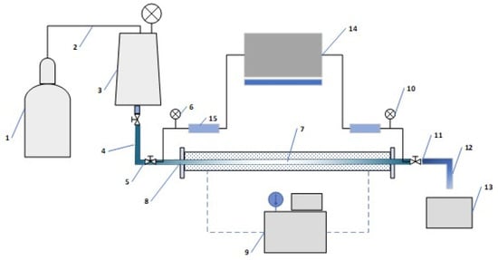
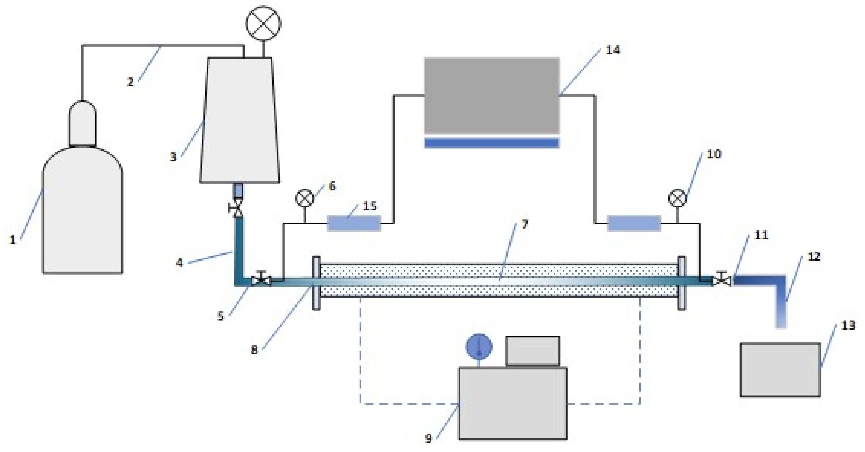
Figure 1 shows a diagram of a laboratory setup consisting of the following elements: 1—gas cylinder with pressure regulator; 2—gas injection line with shut-off valve; 3—saturator/mixing vessel for oil–gas equilibration; 4—oil feed line to the test section; 5—inlet valve to the test tube; 6—inlet pressure transducer; 7—test tube (horizontal pipe section); 8—thermostatic jacket/external thermal bath surrounding the test tube; 9—circulating thermostat unit (temperature control system); 10—outlet pressure transducer; 11—outlet valve; 12—flow meter; 13—outlet separator/collection vessel; 14—data acquisition system (DAQ); 15—temperature sensors (fluid and wall temperatures). The volumetric flow rate was measured using a KATflow 200 hand-held clamp-on ultrasonic flowmeter (Katronic Technologies Ltd., Coventry, UK). The instrument employs the ultrasonic transit-time difference method and allows non-invasive measurement without interrupting the flow or modifying the pipe.

Figure 1. Schematic of the experimental setup for studying the flow of gas-saturated oil in a horizontal tube under controlled external thermal conditions.

Although the experimental setup is laboratory-scale, it represents a physically consistent model of oil transportation through a pipeline under conditions of temperature heterogeneity. The key control mechanisms observed in industrial pipelines—namely, pressure drop along the flow path, heat exchange between the metal pipe wall and the external environment, and, as a result, disruption of the thermodynamic equilibrium of oil and gas—are fully preserved in this setup.

The experimental conditions were chosen to ensure that the relevant dimensionless parameters (Reynolds, Peclet, and supersaturation coefficients) were within the ranges typical for practical oil pipeline operation. Thus, the observed gas separation at the pipe wall and its effect on the pressure drop and flow behavior are directly relevant to real pipeline systems, especially in cold environments and at low flow rates.

The experiments were conducted in a straight horizontal steel tube with a circular cross-section. The test section had an internal diameter of D = 0.004 m, a length of L = 4.0 m. The tube was surrounded by a thermostatic jacket that provided controlled heating or cooling of the pipe wall.

It should be emphasized that the steel test section did not provide optical access to the near-wall region. Therefore, neither the formation of a continuous gas layer nor the local wall-slip velocity was directly visualized or measured. Their occurrence was inferred from the repeatable changes in hydraulic conductance, pressure fluctuations, and flow behavior produced by variations in the temperature difference between the oil and the pipe wall. Consequently, the term “apparent slip” is used here to describe the macroscopic hydrodynamic response consistent with reduced effective wall resistance.

The working fluid was gas-saturated crude oil containing 7 wt.% asphaltenes and a total of 1 wt.% resins and paraffins. The imposed temperature difference between the oil and the pipe wall was varied from 273 to 288 K.

The following procedure was used in our laboratory experiments:

• The required flow rate (or pressure drop) is set and the oil is injected through the test tube.
• Flow curves are taken at different values of the temperature gradient by adjusting the ambient temperature by the circulating thermostat.
• The pressure drop during the flow is maintained constant by means of an automatic regulator at the various pressure levels and the temperature gradients (0–15 K).

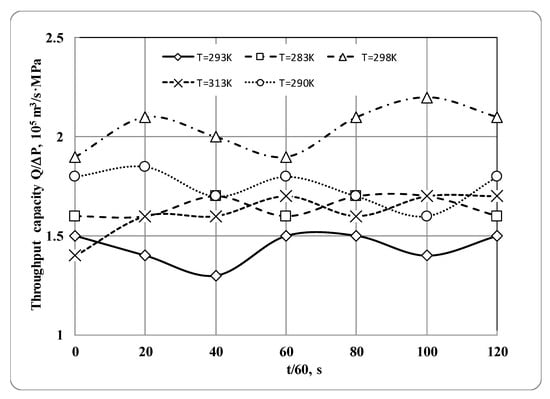
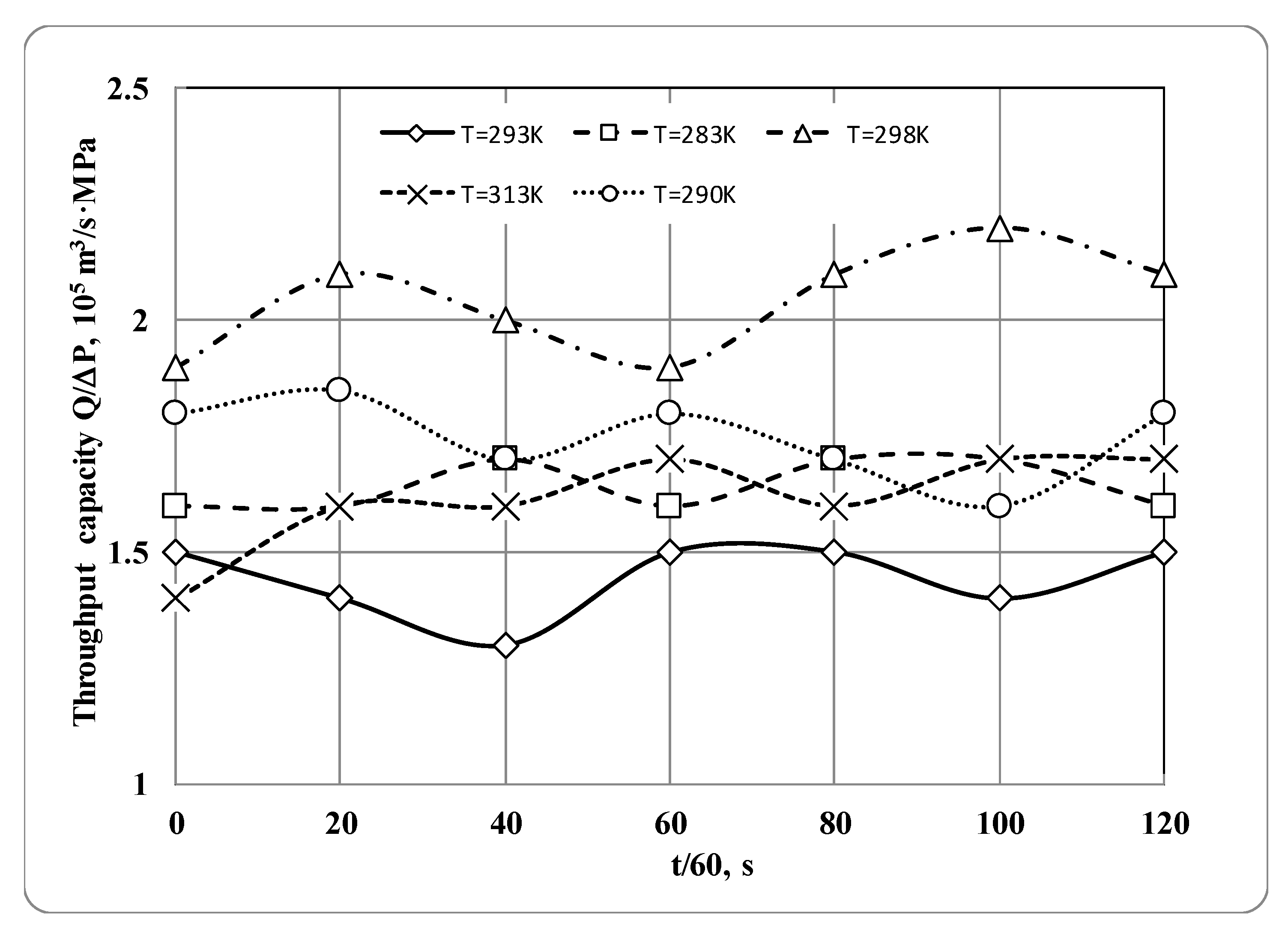
During the experiments, flow curves ($Q-\Delta P$) were taken at various temperature parameters as shown in Figure 2.

Figure 2. Time variation in hydraulic conductance Q/ΔP at different ambient temperatures.

3. Results and Discussions

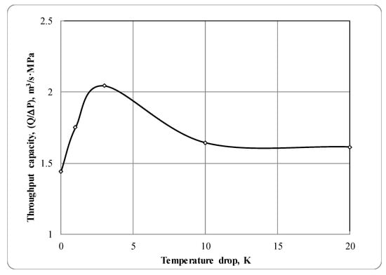
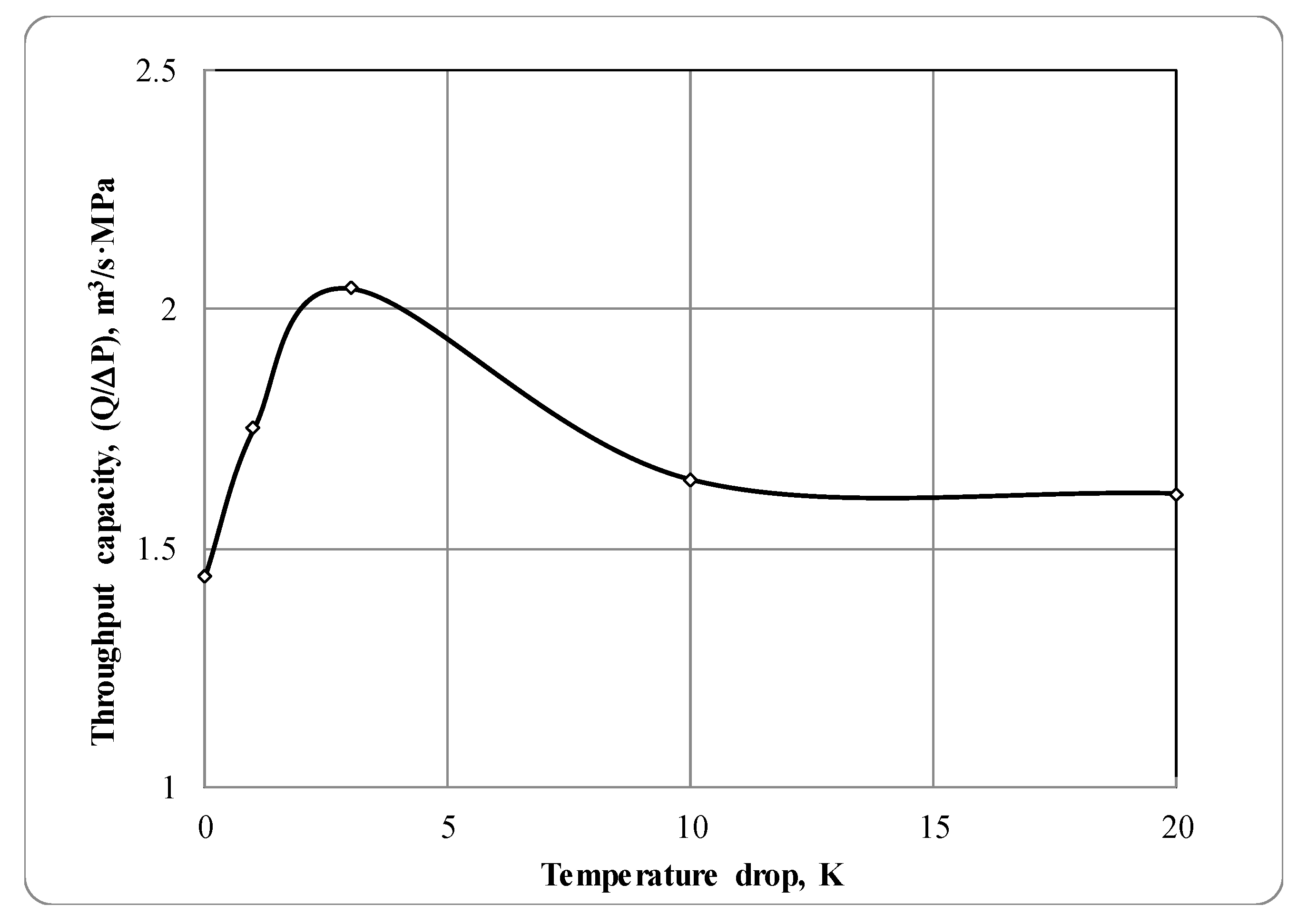
Figure 2 shows the variation in the throughput capacity (hydraulic conductance) with time at various ambient temperatures. Here, Q is the volumetric flow rate with the unit m³/s, and $∆P$ is the pressure drop in MPa. Figure 3 shows the variation in the throughput capacity (hydraulic conductance) with the temperature gradient (difference between inside and outside of the pipe). As we see from these Figures, the throughput capacity of the pipe initially increases with the temperature difference between the oil and the pipe and it reaches a maximum value when the temperature difference is ~5 K. A further increase in the temperature difference results in the declining throughput capacity of the pipe, which starts stabilizing with a temperature difference of 10 K and stays constant as the temperature difference continues to increase. Earlier experimental studies showed that during the pipeline transportation of gas–liquid two-phase flows, continuous gas formation at the interfaces takes place due to the temperature differences between the oil and the pipe wall. This causes high-frequency wavy processes, which cannot be controlled and optimized. This alone introduces further, quite substantial, uncertainties into the operational reliability of the pipeline; That is, the high-frequency vibrations generated can seriously affect the carrying capacity of the pipeline.

Figure 3. Variation in pipe throughput capacity vs. temperature gradient.

Thus, the experimental results provide indirect hydrodynamic evidence consistent with the development of a gas-enriched near-wall region and apparent wall slip. However, they do not constitute a direct visualization or independent quantitative measurement of the gas-layer thickness or slip velocity.

4. Effect of Gas Generation on Hydrodynamic Parameters of Hydrocarbon Fluid Flow

Fluid dynamics effects arising from the gas–liquid joint flow are significantly different compared to the flow of single-phase structures. Research on the main hydrodynamic parameters of the flow of gas–liquid mixtures in pipes is of great importance in the design of the pipeline transport and the technological processes running in the pipeline. Recent studies of gas–liquid flows have shown that even at low liquid flow rates, there is a significant difference between two-phase and single-phase flow. The study of the mutual interaction between the fluid, pipe walls and gas phase—including temperature factor as a limiting state of gas–liquid flow—can be of considerable interest.

Temperature change in pipelines is caused by heat exchange between the environment and the fluid flow. Under known conditions, the temperature can be influenced by various processes: evaporation and condensation of the transported product, gas expansion, hydraulic resistance factor, crystallization and melting of paraffin, etc., as shown by Ogibalov, Ribeiro et al. and Bahrebar et al. [23,24,25].

Studies by Beasley [26] have shown that the emergence of high-frequency wave flows in pipes reduces the reliability of operation on the one hand, and increases the efficiency of oil transport on the other hand.

Fang et al. and Kovarik [11,27] have shown that the generation of active gas centers due to temperature changes between the pipe surface and the transported fluid periodically coincides with the moment of fluctuation manifestation. In horizontal flow, the characteristics of mean and pulsation bubble flow have been widely investigated. However, at low flow rates of such phases, large-scale bubble structures with a high gas concentration are formed along the flow direction.

The hydrodynamic properties of the flow are affected by large-scale gas-foam structures arising along the flow path. In recent years, one has been able to find papers in the literature devoted to experimental studies of large-scale structures in bubble flow. Brodskyi et al. [28] presented their findings regarding the formation of small fluctuations or alternating bubble structures depending on the bubble density. The speed of formation of such structures becomes higher than the average flow velocity.

Joshi et al. [29] showed that small gas bubbles cluster in a chain, forming bubble regions that will then move together in a wave-like fashion. Large-scale vortex structures are formed between the channel wall and the ‘ribbon’ of bubbles, which create flows in opposite directions within the flow, as shown by Yan et al. [30].

Astarita et al. [31] note that fluctuations lead to the formation of thin 10⁻⁵ m liquid microlayers between the gas bubbles and the surface, and to their rapid disappearance. Given these generation periods, it is possible to estimate the local heat transfer cases using information on the periods of primary gas bubble formation. The following well-known equations of Astarita et al. [31] are used for the influence of internal processes in the pipe on the temperature:

$$t_k=t_0+\left(t_n-t_0\right)e^{-a}$$

(5)

$$a={\displaystyle \frac{K\pi dL}{GC}}$$

(6)

where $t_H$, $t_K$ and $t_0$—ambient temperatures at the initial and final points of the flow in the pipe, respectively; K—total heat transfer coefficient from the flow to the environment; D and L—pipe diameter and length; and G—mass heat capacity of the mixture.

It should be noted that Equations (5) and (6) include a fixed value of the K—heat transfer coefficient which does not take into account heat losses along the pipe length. Otherwise, the following expression is given by Chernikin for the following case [14]:

$$a={\displaystyle \frac{K\pi dL}{G(C\pm C^0)}}$$

(7)

where a is the amount of heat released (+K) or absorbed (−K) in 1.0 kg of product when the temperature changes by 1 K, as shown by Chen [32].

Equations (5) and (6), obtained for a single-phase flow, can also be used for a gas–liquid mixture. The only difference may be in finding the heat capacity and thermal conductivity coefficients. The heat transfer coefficient takes into account the whole complex process of heat conduction and is determined by the condition of heat exchange of the temperature of the flowing product with the environment through the pipe wall. This is described by the following expression proposed by Chernikin in [14]:

$${\displaystyle \frac{1}{k{d}_{BH}}}={\displaystyle \frac{1}{{\alpha }_1{D}_{BH}}}+\sum {\displaystyle \frac{\ln \frac{d_H}{d_{BH}}}{2\lambda }}+{\displaystyle \frac{1}{{\alpha }_2{D}_H}},$$

(8)

where

${\alpha }_1$—internal heat transfer coefficient (heat transfer from the flow to the pipe walls);

${\alpha }_2$—external heat transfer coefficient (heat transfer from the pipe wall to the environment);

D_in and D_o are the outside diameter of the pipe together with the inside diameter and, respectively, with insulation;

$\lambda$—heat conductivity coefficient of the pipe and insulation.

As shown by Chen and Cui [32,33], the characterization of a two-phase flow is affected only by its internal heat transfer coefficient ${\alpha }_1$. For hydrocarbon system transport conditions, the thermal resistance of gas bubbles formed at the interface between the liquid and the metallic inner surface of the pipe has a great effect. The number of active centers transforming into gas bubbles depended on the pipe material and the temperature difference, which increases even more with their increase. If the temperature difference exceeds the critical temperature θ_0max, typically (5–10 K), gas bubbles often accumulate near the tube surface. At this time, the pipe surface is covered by a roughly ordinary gas layer. This results in thermal insulation and a reduction in the intensity of the temperature flux. The thickness of the thermal insulating micro-layer adjacent to the gas bubbles can be found from the following equation [16]:

$$-C{\displaystyle \frac{d\theta }{dt}}=hA\theta$$

(9)

where $C=V_{{\rho }_1}C$—heat capacity of gas bubbles; $C$—specific heat capacity of a bubble; h—coefficient of stationary temperature transfer, $V=Ad=4\pi b{R}^{2}d$; V—bubble volume; and b—bubble growth parameter.

Under these conditions, Equation (9) is reduced to the following form:

$$-{\displaystyle \frac{d\theta }{dt}}={\displaystyle \frac{h}{{\rho }_{1}cd}}\theta ;l_n\theta ={\displaystyle \frac{h}{{\rho }_{1}cd}}i$$

(10)

$\theta$—temperature; d—gas microlayer thickness; and D—some transformations were obtained by van Stralen [5]:

$$d(t)={\displaystyle \frac{{\rho }_{2}l}{{\rho }_{1}C}}{C}_1\left(t_1-t\right)$$

(11)

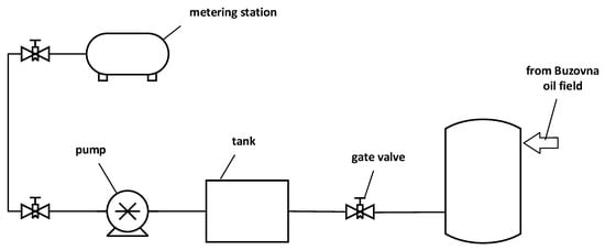
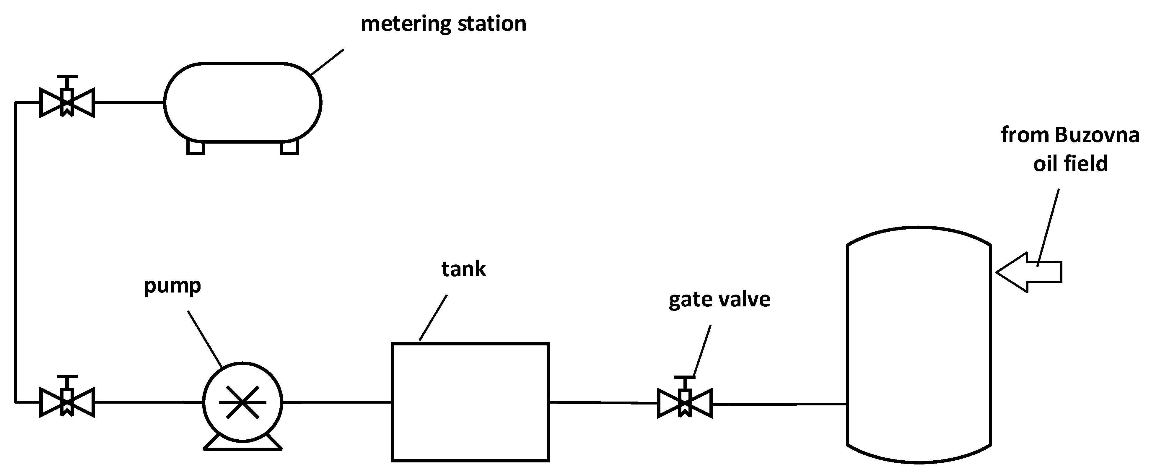
The test fluid was transported through the pump CNZV200x2 from the reservoir at a constant temperature (T = 313 K) through 198 km long and 0.2 m diameter pipeline to the Sabunchi pumping station (Baku, Azerbaijan) (Figure 4). The process parameters in these pilot field tests were measured in two-hour time intervals. The physical and chemical characteristics of the test oil are shown in Table 1.

Figure 4. Schematic diagram of the Buzovna–Sabunchi oil field (Azerbaijan) pipeline capacity study.

Table 1. Physical and chemical characteristics of transported oil.

Density, kg/m3	Viscosity, Pa·s	Paraffins, %	Resins, %	Asphaltenes, %	Water, %	Impurities, %	Chlorides, %	Gas Factor, m3/m3
0.91	0.159	0.75	11	0.14	0.18	0.03	0.05	0.2

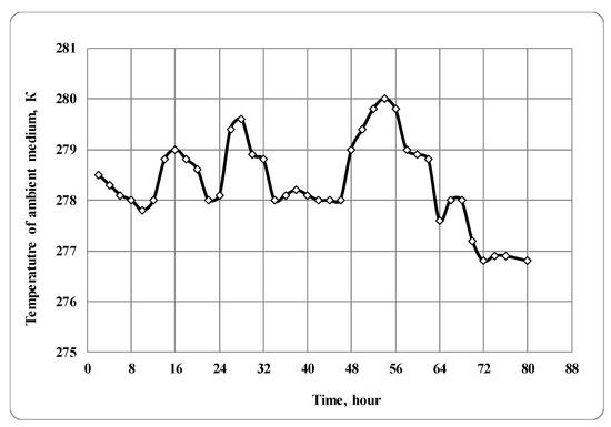
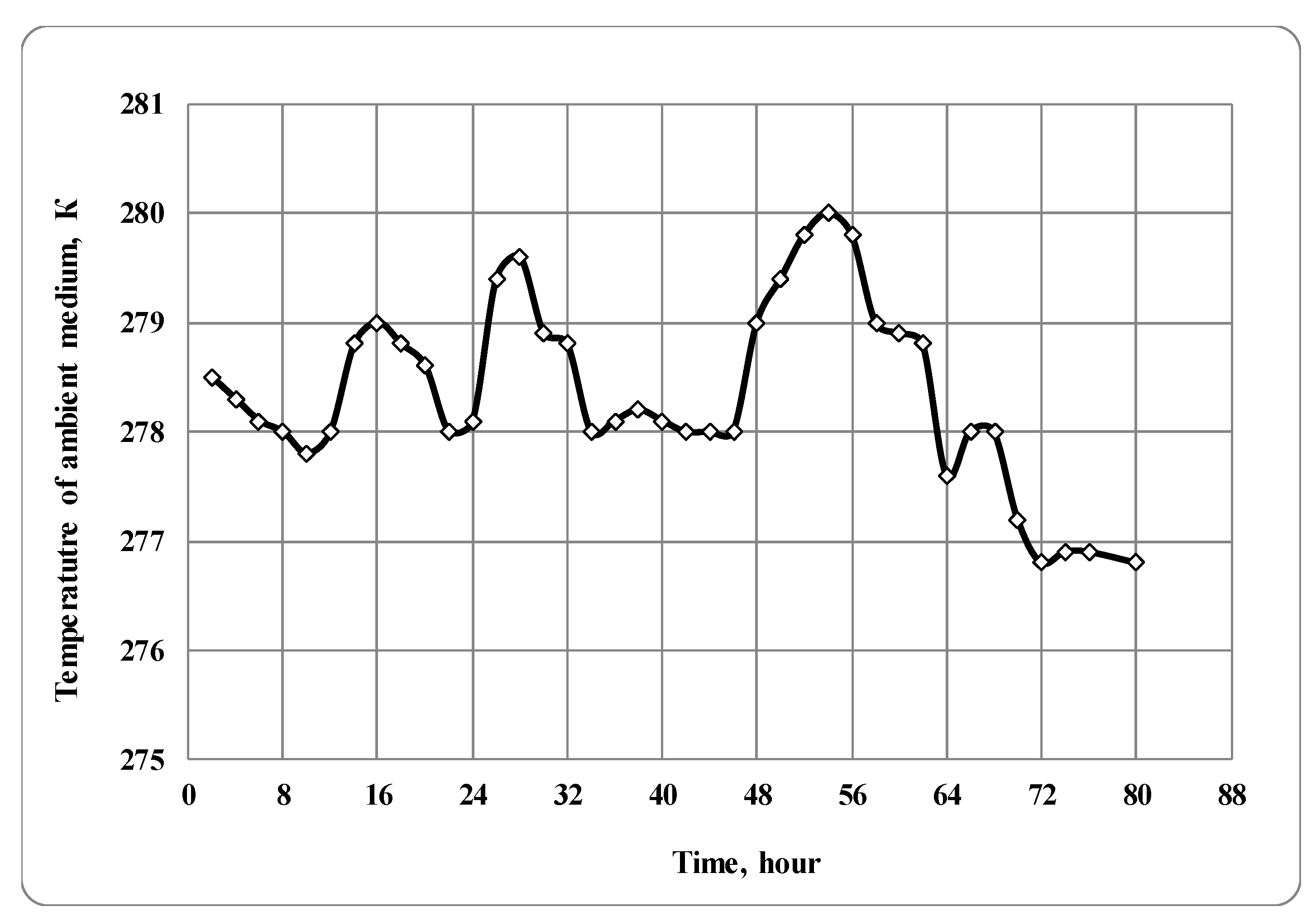
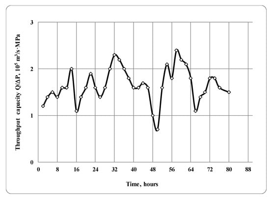
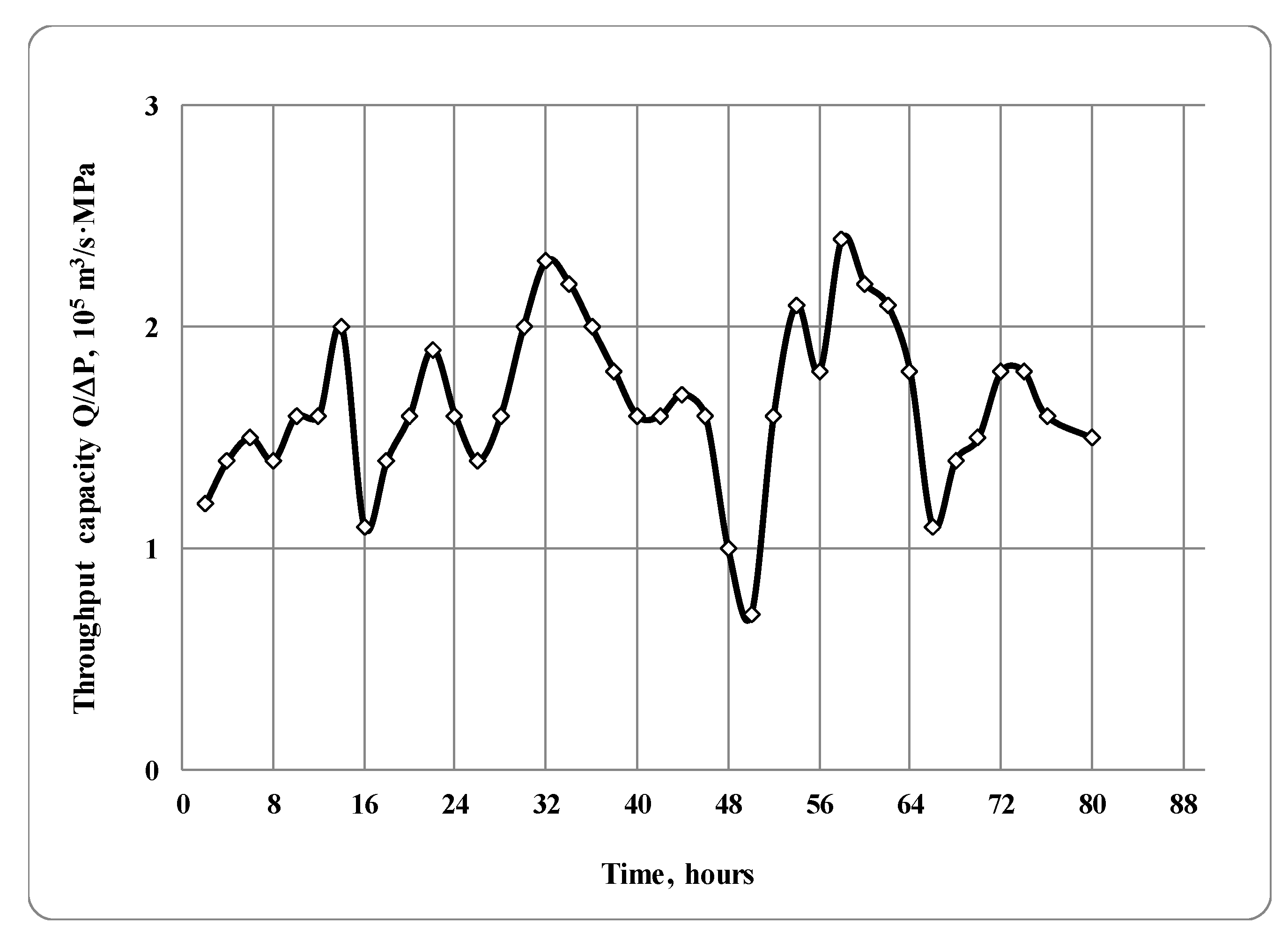
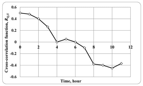
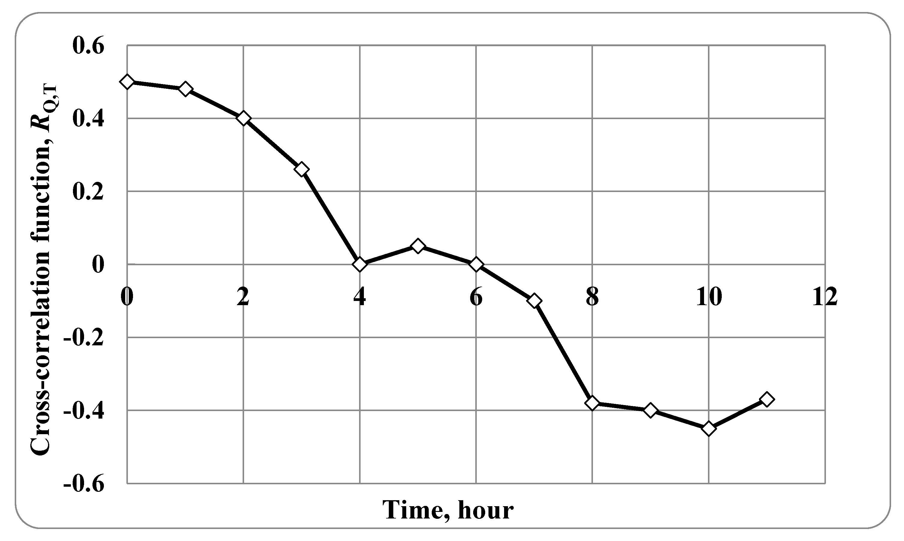
Figure 5 and Figure 6 show an oscillatory character of the variations in both the temperature and the throughput capacity of the pipe with time. Therefore, one would assume that it is impossible to establish a direct relationship between these parameters. To determine the influence of the ambient temperature changes on the pipe throughput, the values of their mutual correlation function on the exposure were calculated and they are shown in Figure 7.

Figure 5. Ambient temperature change.

Figure 6. Variation in pipeline throughput capacity with time.

Figure 7. Time-dependent correlation of pipe capacity and ambient temperature change.

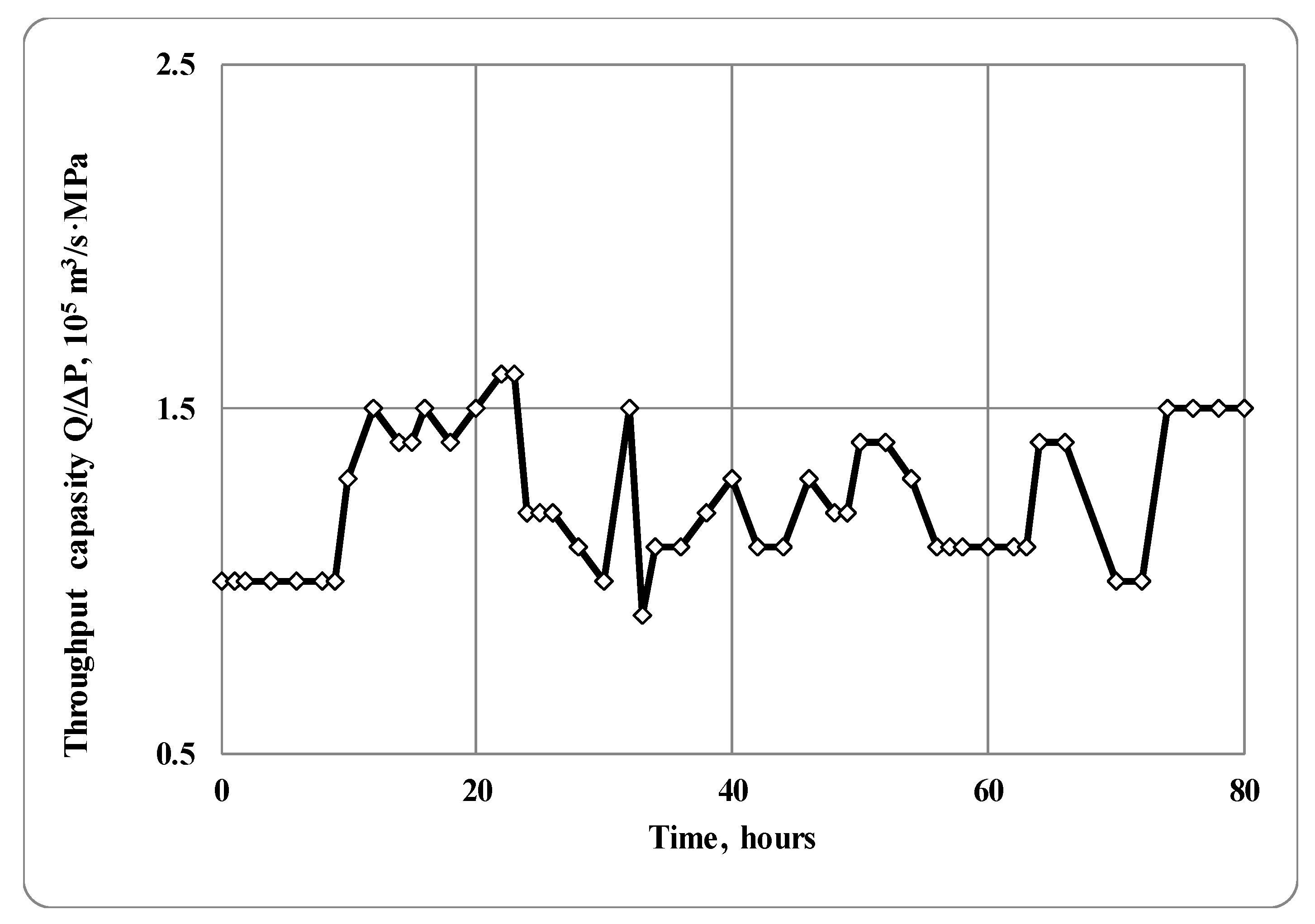
Figure 7 shows that the maximum value of the cross-correlation function does not exceed 0.48. This also indicates that there is no relationship between temperature change and pipe throughput. The pilot field tests also were conducted to confirm the time dependence of the throughput capacity of the pipe. Under small temperature gradients between the fluid flow in oil pipeline and the surrounding environment (T = 303 K), a variation in the throughput capacity in real time was recorded during these pilot tests (Figure 8).

Figure 8. Variation in pipe throughput capacity as a function of time.

As seen in Figure 8, the throughput capacity of the pipeline in the transported gas and fluid systems at the temperatures equal the ambient temperature is characterized by weak fluctuations. Under these conditions, the throughput of the pipe is slightly less than that under conditions other than ambient temperature. However, we note that a very important factor in the pipe throughput capacity is the slip effect, due to the layer formed by gas bubbles on the surface of the pipe wall. A number of studies [34,35,36] confirmed the formation of gas bubbles on the surface of pipe walls, which may decrease the hydraulic resistance of the transported fluids.

5. Conclusions

This paper presents the results of the study of the transport process of the fluid flow through a pipeline under various temperature gradients between the internal and external environments and continuous gas generation at the contact boundary of the media. The test results demonstrated that under the non-isothermal flow case, a slippage effect will significantly affect the flow velocity, the pressure and the temperature distributions in the variable cross-section pipes. Laboratory experiments were also performed to study the effects of the gas nucleus at the pipe walls on the hydrodynamic characteristics of the flow. A new approach was applied in the study, which consists of a combination of methods for determining slip limits and threshold slip in non-isothermal experiments with a relatively constant pressure drop. A technique is proposed that allows the simultaneous measurement of oil temperature and pipe wall, pressure drop, and volumetric flow rate. This allowed us to determine the initial, peak, and subsequent stages of attenuation of the slippage effect.

The test results showed that the throughput capacity of the pipe is considerably affected by the temperature difference between the fluid and the pipe walls. At certain temperature gradients on the border layer, the pipe capacity reaches a maximum value. In particular, the hydraulic conductivity Q/ΔP increased from approximately 1.45 × 10⁻⁵ m³/(s·MPa) at ΔT = 0 K to approximately 2.04 × 10⁻⁵ m³/(s·MPa) at ΔT ≈ 3–5 K, representing an increase of about 41%. At ΔT = 10 K, the conductivity decreased to approximately 1.64 × 10⁻⁵ m³/(s·MPa), which is about 20% lower than its maximum value, and subsequently stabilized within the range of approximately (1.60–1.64) × 10⁻³ m³/(s·MPa). The initial increase is consistent with the formation of a gas-saturated zone near the wall and the resulting reduction in the effective resistance of the wall. The subsequent decline and steadiness can be explained by the accumulation of gas, the thermal insulation of the adjacent layer, and the increased disturbances in the two-phase flow.

Future research studies must be focused on the identification of the reasons for the origin of these high-frequency vibrations, the range of possible frequencies and amplitudes of the temperature fluctuations, and the selection of the insulating coatings with lowest thermal conductivity.

The conducted research has confirmed the importance of accounting for heat transfer processes under thermal instability conditions when managing the throughput capacity of pipelines used for gas–liquid mixture transportation. The efficiency of multiphase flow transport is essentially determined by the thermophysical properties of the gas phase, with key parameters being the thermal conductivity coefficient and the thickness of the gas layer. Understanding the regularities of heat and mass transfer and their impact on flow dynamics provides a basis for optimizing design solutions for transporting multiphase systems under variable thermobaric conditions. This would enable more accurate control of flow regimes and improve the operational reliability of pipeline systems.

During field tests, which were conducted on a 198 km long and 0.2 m diameter pipeline section, it was found that the correlation coefficient between temperature and throughput did not exceed 0.48. This indicates that the pipeline capacity is affected not only by temperature conditions, but also by other factors such as heat transfer, gas release, gas accumulation at the walls and the characteristics of the two-phase flow.

References

- Neto, C.; Evans, D.R.; Bonaccurso, E.; Butt, H.-J.; Craig, V.S.J. Boundary slip in Newtonian liquids: A review of experimental studies. Rep. Prog. Phys. 2005, 68, 2859–2897. [Google Scholar] [CrossRef] [Scilit]
- Yankov, V.I.; Boyarchenko, V.I.; Pervadchuk, V.P.; Glot, I.O.; Shakirov, N.V. Processing of fiber-forming polymers: Fundamentals of polymer rheology and polymer flow in channels. In Regular and Chaotic Dynamics; Institute of Computer Science: Izhevsk, Russia, 2008. [Google Scholar]
- Rao, I.J.; Rajagopal, K.R. The effect of the slip boundary condition on the flow of fluids in a channel. Acta Mech. 1999, 135, 113–126. [Google Scholar] [CrossRef] [Scilit]
- Bahrami, M.; Tamayol, A.; Taheri, P. Slip-flow pressure drop in microchannels of general cross section. J. Fluids Eng. 2009, 131, 031201. [Google Scholar] [CrossRef] [Scilit]
- van Stralen, S.J.D.; Zijl, W. Fundamental developments in bubble dynamics. In Proceedings of the 6th International Heat Transfer Conference, Toronto, ON, Canada, 7–11 August 1978; pp. 429–447. [Google Scholar]
- Borzenko, E.I.; Dyakova, O.A.; Shrager, G.R. Investigation of the slip phenomenon in viscous fluid flow through a curved channel. Vestn. Tomsk. Gos. Univ. Mat. I Mekhanika 2014, 2, 35–44. (In Russian) [Google Scholar]
- Minakov, A.V.; Rudyak, V.Y.; Dekterev, A.A.; Gavrilov, A.A. Investigation of slip boundary conditions in the T-shaped microchannel. Int. J. Heat Fluid Flow 2013, 43, 161–169. [Google Scholar] [CrossRef] [Scilit]
- Hooman, K.; Hooman, F.; Famouri, M. Scaling effects for flow in micro-channels: Variable properties, viscous heating, velocity slip, and temperature jump. Int. Commun. Heat Mass Transf. 2009, 36, 192–196. [Google Scholar] [CrossRef] [Scilit]
- Scriven, L.E. On dynamics of phase growth. Chem. Eng. Sci. 1959, 10, 1–13. [Google Scholar] [CrossRef] [Scilit]
- Arnautovic, Z.; Welzl, M.; Heberle, F.; Brüggemann, D. Enhanced heat transfer correlation for nucleate boiling of fluid mixtures. Int. J. Heat Mass Transf. 2024, 231, 125804. [Google Scholar] [CrossRef] [Scilit]
- Fang, S.; Zhou, C.; Zhu, Y.; Qian, Z.; Wang, C. Review on Research Progress of Pulsating Heat Pipes. Inventions 2024, 9, 86. [Google Scholar] [CrossRef] [Scilit]
- Mamaev, V.A.; Odishariya, G.E.; Semenov, N.I.; Tochigin, A.A. Hydrodynamics of Gas-Liquid Mixtures in Pipes; Nedra Publ.: Moscow, Russia, 1969. (In Russian) [Google Scholar]
- Afanasyev, V.M. Pipelines simulations for transportation of gas-liquid mixture. J. Oil Bus. 1962. (In Russian) [Google Scholar]
- Chernikin, V.I. Gidrotransport vyazkikh neftey po truboprovodam. Neft. Khozyaystvo 1965, 7, 56–59. (In Russian) [Google Scholar]
- Hong, B.Y.; Liu, S.N.; Li, X.P.; Fan, D.; Ji, S.P.; Chen, S.H.; Li, C.C.; Gong, J. A liquid loading prediction method of gas pipeline based on machine learning. Pet. Sci. 2022, 19, 3004–3015. [Google Scholar] [CrossRef] [Scilit]
- Dammer, S.M.; Lohse, D. Gas enrichment at liquid-wall interfaces. Phys. Rev. Lett. 2006, 96, 206101. [Google Scholar] [CrossRef] [Scilit] [PubMed]
- Forster, H.K.; Zuber, N. Growth of vapor bubble in superheated liquid. J. Appl. Phys. 1954, 25, 474–478. [Google Scholar] [CrossRef] [Scilit]
- Falcone, G.; Teodoriu, C.; Reinicke, K.M.; Bello, O.O. Multiphase-flow modeling based on experimental testing: An overview of research facilities worldwide and the need for future developments. SPE Proj. Facil. Constr. 2008, 3, 1–10. [Google Scholar] [CrossRef] [Scilit]
- Faraji, F.; Santim, C.; Chong, P.L.; Hamad, F. Two-phase flow pressure drop modelling in horizontal pipes with different diameters. Nucl. Eng. Des. 2022, 395, 111863. [Google Scholar] [CrossRef] [Scilit]
- Malekzadeh, R.; Henkes, R.A.W.M.; Mudde, R.F. Experimental study of flow instabilities in a hilly-terrain pipeline/riser system. SPE J. 2013, 18, 179–188. [Google Scholar]
- Wang, Z.; Zhang, Q.; Zeng, Q.; Wei, J. A unified model of oil/water two-phase flow in the horizontal wellbore. SPE J. 2016, 22, 353–364. [Google Scholar] [CrossRef] [Scilit]
- Magrini, K.L.; Sarica, C.; Al-Sarkhi, A.; Zhang, H.Q. Liquid entrainment in annular gas/liquid flow in inclined pipes. SPE J. 2012, 17, 617–630. [Google Scholar] [CrossRef] [Scilit]
- Ogibalov, P.M.; Mirzadzhanzade, A.H. Mekhanika Fizicheskikh Protsessov; MGU Press: Moscow, Russia, 1976. (In Russian) [Google Scholar]
- Ribeiro, D.; Santos, L.; Romero, O. Heavy oil transportation through steam heating: An analytical and numerical approach. J. Pet. Sci. Eng. 2020, 195, 107932. [Google Scholar] [CrossRef] [Scilit]
- Bahrebar, S.; Ambat, R. Investigation of critical factors effect to predict leakage current and time to failure due to ECM on PCB under humidity. Microelectron. Reliab. 2021, 127, 114418. [Google Scholar] [CrossRef] [Scilit]
- Beasley, C.; Castel, B.; Zimmerman, T.; Lestz, R.; Yoshioka, K.; Long, A.; Lutz, S.J.; Riedel, K.; Sheppard, M.; Sood, S. Mining heat. Oilfield Rev. 2010, 21, 4–13. [Google Scholar] [CrossRef] [Scilit]
- Kovarik, B. The oil reserve fallacy: Proven reserves are not a measure of future supply. In Proceedings of the International Communication Association (ICA) Annual Meeting, Boston, MA, USA, 26–30 May 2011. [Google Scholar]
- Brodskyi, Y.; Gyrya, V.; Zlotnik, A. Simulation of gas mixture dynamics in a pipeline network using explicit staggered-grid discretization. Appl. Math. Model. 2025, 137, 115717. [Google Scholar] [CrossRef] [Scilit]
- Joshi, J.B.; Pandit, A.B.; Kataria, K.L.; Kulkarni, R.P.; Sawarkar, A.N.; Tandon, D.; Ram, Y.; Kumar, M.M. Petroleum residue upgradation via visbreaking: A review. Ind. Eng. Chem. Res. 2008, 47, 8960–8988. [Google Scholar] [CrossRef] [Scilit]
- Yan, Y.; Wang, L.; Chen, J. A mesoscale bubble-induced turbulence model and simulation of gas–liquid flows. Phys. Fluids 2023, 35, 013314. [Google Scholar] [CrossRef] [Scilit]
- Astarita, G.; Marrucci, G.; Joseph, D. Principles of Non-Newtonian Fluid Mechanics; McGraw-Hill: London, UK; New York, NY, USA, 1974; ISBN 0070840229. [Google Scholar]
- Chen, L.W. A theoretical and experimental study on flow characterisation in an acoustically excited chamber. Wave Motion 2015, 58, 68–76. [Google Scholar] [CrossRef] [Scilit]
- Cui, G. Research on oil-gas gathering and transportation process technology in Qingdong-5 zone. Pet. Sci. Technol. 2016, 57, 339–346. [Google Scholar]
- Kaloni, P.N.; Qiao, Z. Nonlinear convection with inclined temperature gradient and horizontal mass flow. Int. J. Eng. Sci. 1997, 35, 299–309. [Google Scholar] [CrossRef] [Scilit]
- Nasehi, M.; Asghari, K. Use of CO2 in heavy-oil waterflooding. In Proceedings of the SPE International Conference on CO2 Capture, Storage, and Utilization, New Orleans, LA, USA, 12 November 2010; pp. 474–486. [Google Scholar]
- Yuan, H.; Zhou, D. Evaluation of two-phase flow correlations and mechanistic models for small-diameter pipelines at slightly inclined downward flow. SPE Proj. Facil. Constr. 2010, 5, 5–12. [Google Scholar] [CrossRef] [Scilit]
Disclaimer/Publisher’s Note: The statements, opinions and data contained in all publications are solely those of the individual author(s) and contributor(s) and not of MDPI and/or the editor(s). MDPI and/or the editor(s) disclaim responsibility for any injury to people or property resulting from any ideas, methods, instructions or products referred to in the content. |
© 2026 by the authors. Licensee MDPI, Basel, Switzerland. This article is an open access article distributed under the terms and conditions of the Creative Commons Attribution (CC BY) license.