


Abstract
We investigate the information-geometric structure of a self-consistent second-virial approximation with the van der Waals form of the second virial coefficient, using the Fisher information as a generating potential. By constructing the associated Hessian metric and scalar curvature, we obtain a geometric description of thermodynamic fluctuations that complements the standard equation-of-state approach. We show that interaction effects enter the Fisher information selectively through their temperature dependence, with attractive interactions playing the dominant role while excluded-volume contributions remain subleading. The Hessian determinant of the Fisher information changes sign along well-defined crossover loci in the reduced parameter space, separating regions of saddle-like and locally convex curvature of the fluctuation landscape, and diverges as at the closure boundary. The scalar curvature diverges at the closure boundary as a simple pole, with a leading term that is universal and independent of the interaction parameters. We derive its exact closed-form expression, which shows that the curvature is negative for weak-to-moderate effective coupling but turns positive in the strong-coupling regime, where the underlying Fisher–Rao metric loses positive-definiteness. The curvature diverges on approach to this metric boundary, which lies strictly inside the mechanically stable region, short of the closure boundary itself. These results demonstrate that Fisher geometry provides a selective probe of interaction-induced fluctuations, capturing how thermal states reorganize under temperature variations rather than encoding phase transitions directly. This approach offers a complementary perspective on interacting systems and suggests new avenues for extending information-geometric methods to more strongly correlated and quantum regimes.
1. Introduction
The geometrization of thermodynamics and statistical mechanics has provided deep insight into the structure of fluctuations and interactions in many-body systems. Beginning with the foundational work of Rao [1] and Fisher, probability distributions can be endowed with a Riemannian metric that quantifies statistical distinguishability. This framework, later formalized as information geometry [2], has found widespread applications in physics, particularly in the study of equilibrium thermodynamics.
In parallel, geometric approaches to thermodynamics were developed by Weinhold [3] and Ruppeiner [4], who introduced metric structures on the space of equilibrium states. Within Ruppeiner’s formulation, the scalar curvature has been interpreted as a measure of correlations in the underlying system, providing a powerful diagnostic of interactions and critical phenomena [5,6]. In particular, curvature singularities have been associated with phase transitions, while its sign has been linked to the effective nature of interactions.
More recently, increasing attention has been devoted to the role of information-theoretic quantities, such as the Fisher information, in thermodynamics. In equilibrium systems, the Fisher information with respect to temperature is directly related to energy fluctuations, establishing a bridge between statistical estimation theory and thermodynamic response [7,8]. This connection has led to the concept of thermodynamic length and to bounds on dissipation in nonequilibrium processes [9], further highlighting the physical relevance of information geometry.
Despite these advances, the role of Fisher information in interacting classical systems has received comparatively less attention than the Weinhold/Ruppeiner framework, and it remains only partially understood how microscopic interactions manifest themselves in the information-geometric structure of thermodynamic state space. Equation-of-state-based approaches characterize how interactions modify macroscopic response functions, but have paid comparatively less attention to the complementary question of how interactions affect the distinguishabilitybetween nearby statistical states, which is the focus of the present work.
In this work, we investigate this question using a self-consistent second-virial approximation with the van der Waals form of the second virial coefficient, , one of the simplest and most paradigmatic parametrizations of interacting fluids [10,11,12,13,14]. By combining the virial expansion with information-geometric methods, we derive explicit expressions for the Fisher information, its Hessian structure, and the associated scalar curvature. This allows us to analyze how interactions shape the geometry of fluctuations in a controlled and analytically tractable setting.
Our results reveal several nontrivial features. First, interaction effects enter the Fisher information exclusively through derivatives of the second virial coefficient, indicating that Fisher geometry probes the thermal sensitivity of interactions rather than their static magnitude. Second, we find that the Fisher information is insensitive to the excluded-volume parameter, highlighting a selective sensitivity to energetic correlations. Third, the Hessian of the Fisher information changes sign along well-defined crossover loci in the reduced parameter space, separating regions of saddle-like and locally convex curvature of the fluctuation landscape. Finally, the scalar curvature admits an exact closed form with a universal leading term, , that would formally diverge as a simple pole at the closure boundary (referred to as “spinodal-like” below, in the restricted sense defined in Section 2, where its relation to a genuine finite-density thermodynamic instability is discussed); it is negative for weak-to-moderate effective coupling but turns positive in the strong-coupling regime, at low reduced temperature and density, before diverging on approach to the boundary where the underlying Fisher–Rao metric loses positive-definiteness—a locus that lies strictly inside the mechanically stable region, short of itself.
These findings provide a complementary perspective on interacting systems, in which the focus shifts from thermodynamic potentials to the geometry of fluctuations. Within this framework, interactions are characterized by how they modify the distinguishability between nearby thermal states, offering a new lens through which to analyze classical fluids.
The paper is organized as follows: Section 2 establishes the grand canonical framework and the self-consistent virial approximation. Section 3 derives the Fisher information and links it to macroscopic energy fluctuations. In Section 4, we introduce reduced variables to uncover universal scaling laws. Section 5 investigates the Hessian of the Fisher information and identifies geometric crossover loci in the stable region. Section 6 extends this to intrinsic geometry by computing the Ricci scalar curvature and its scaling near the closure boundary . Finally, Section 7 and Section 8 provide a summary of results and concluding remarks.
2. Grand Canonical Framework
We consider a classical interacting system described within the grand canonical ensemble, characterized by the grand partition function [15,16]
where
is the canonical partition function [15]. Here is the fugacity and is the thermal wavelength [15]. The configurational integral is given by [15,16,17]
where the normalization ensures that in the ideal gas limit.
2.1. Second Virial Approximation and Mean-Field Closure
For a dilute interacting gas, the configurational integral admits a virial expansion. Retaining only the second virial contribution, one obtains the standard approximation [16,17]
In order to proceed analytically within the grand canonical ensemble, we further introduce a mean-field closure in which the instantaneous density is replaced by a self-consistent mean-field parameter [15]. This yields the approximate form
which captures interaction effects at the level of the second virial coefficient while allowing for a closed-form evaluation of .
With this approximation, the grand partition function becomes [15,16,17]
2.2. Self-Consistent Density
Self-consistency of the mean-field closure requires that the parameter n entering Equation (5) coincide with the mean particle number computed at fixed n — i.e., before the implicit dependence is taken into account. Holding n fixed, the trial grand potential is linear in z, so that
Imposing self-consistency—i.e., requiring this quantity to equal —yields the implicit equation for the density
Equation (8) defines n as a self-consistent function of . Using Equation (8), one can rewrite
which becomes an exact identity within the present mean-field closure [15,16,17].
It is important to stress that, once is regarded as the implicit solution of Equation (8), Equation (9) is an exact function of z alone (at fixed ), and the true mean particle number must be obtained by differentiating Equation (9) including the implicit z-dependence of n. Simply reading off Equation (9) would amount to treating n as z-independent, which contradicts Equation (8) itself. Introducing , so that , and differentiating implicitly with respect to at fixed gives
where we introduce, once and for all, the control parameter
which will be used throughout this work (bare, as “D”, whenever the functional dependence is clear from context) as a unified control parameter governing stability, response functions, and information geometry.
Therefore the mean-field parameter n solving Equation (8) is not itself the physical mean density: the latter is given exactly by
which coincides with n only in the dilute limit , where . The direct thermodynamic interpretation of D implied by Equation (13) is made explicit below, once the equation of state has been derived.
2.3. Mean Energy
The mean energy is given by the standard grand canonical relation [15,16]
Since depends implicitly on , the derivative must be computed consistently. Using Equation (8), one obtains
Differentiating Equation (8) with respect to at fixed z, and defining , we find
which leads to the final expression
2.4. Virial Equation of State and Self-Consistency
The equation of state can be derived from the grand potential. To ensure consistency with the self-consistent density defined in Equation (8), we invoke the Gibbs–Duhem relation at constant temperature, [16], where is the physical mean density given by Equation (13). Recalling that , we have at fixed T, so that
where the last step uses Equation (10). Integrating Equation (18), and imposing the ideal-gas limit as , gives
Unlike the response functions considered below (, , ), the pressure carries no singular dependence on the control parameter D and remains regular at (see below for the precise meaning of this boundary).
Equation (13), , can be solved exactly for n:
Substituting Equation (20) into Equation (19) gives the equation of state in terms of the physical density,
which, expanded for , recovers the standard second virial expansion
We stress that , as it appears in Equations (20) and (21), is not a conventional van der Waals spinodal. For finite physical density , Equation (20) shows that can never vanish; instead corresponds to (for ). Correspondingly, differentiating Equation (21) gives
identically, for all finite : unlike the genuine van der Waals loop, the present self-consistent closure yields a pressure that is strictly monotonic in the physical density, with no interior extremum. The condition is therefore better understood as a singular boundary of the self-consistent closure itself—the locus where the map between the mean-field parameter and the physical density breaks down—rather than a finite-density mechanical instability of the conventional van der Waals type. We nonetheless refer to below as a spinodal-like closure boundary, in this restricted sense, to denote the divergence of response functions and information-geometric quantities associated with it, without implying the existence of a genuine liquid–gas instability at finite density; the term “spinodal” unqualified is reserved for the conventional finite-density instability, which the present closure does not reproduce.
2.5. D as the Compressibility Factor
Combining the exact equation of state, Equation (19), with Equation (13) gives a direct thermodynamic interpretation of the control parameter D introduced in Equation (11):
i.e., D coincides exactly with the compressibility factor Z of the fluid. Thus D provides a direct measure of the deviation from ideal-gas behavior: corresponds to the ideal-gas limit, while deviations of D from unity quantify the effect of interactions on the equation of state.
2.6. Compressibility and the Closure Boundary
The isothermal compressibility provides the standard diagnostic of mechanical stability [15,17,18]: for a fluid system, mechanical stability requires to be positive, defined in terms of the physical mean density [Equation (13)]:
To evaluate within the present closure, it is convenient to use n as the independent variable and apply the chain rule,
From the exact equation of state, Equation (19), , so that
From Equation (13), , so that
Combining these results, and using ,
Equation (29) diverges () as , i.e., at the closure boundary discussed above rather than at a finite-density thermodynamic instability. From an information-geometric perspective, this same condition defines a singularity where the Fisher information metric diverges, reflecting the system’s infinite sensitivity to infinitesimal changes in thermodynamic coordinates.
Crucially, is physically accessible only if . This occurs exclusively at temperatures below the Boyle temperature (), where attractive interactions prevail. For , we have , meaning , and the system remains unconditionally stable within the second virial approximation.
3. Interacting Gas: Second Virial Approximation
3.1. Fisher Information
The Fisher information with respect to the inverse temperature at fixed fugacity z is defined as [7,19,20]
This quantity measures the variance of energy fluctuations, . Within the second virial approximation, the Fisher information takes the form
where the density-dependent factor is given by
and [Equation (11)] is the stability control parameter. For the van der Waals form of the second virial coefficient, , so that and ; specializing the control parameter of Equation (11) accordingly gives
which we use throughout the remainder of this work whenever the explicit van der Waals form is needed. With , Equation (32) reduces to
As the system approaches the closure boundary , the Fisher information diverges as , signaling that the energy fluctuations become macroscopic there. This cubic divergence, together with the requirement that as a genuine energy-fluctuation variance, is discussed further in Appendix A, where it is shown to fail once the interaction is strong enough even within the mechanically stable region .
3.2. Comments on the Fisher Information
3.2.1. Key Physical Insight
Interaction effects enter the Fisher information through both and its derivatives. However, the genuinely new contributions to energy fluctuations arise from the temperature derivatives of the second virial coefficient. This shows that Fisher geometry probes the thermal sensitivity of interactions rather than their static contribution, providing access to features of the system that remain hidden in conventional approaches.
3.2.2. Selective Sensitivity to Interactions
At leading order in the dilute regime, the interaction-dependent contribution to the reduced Fisher information depends only on the attractive parameter a (since ), while the excluded-volume parameter b enters only through the self-consistent control factor , not through the explicit derivative structure of . This shows that Fisher information selectively probes energetic correlations through the thermal derivatives of the interaction, while remaining insensitive, at this order, to the geometric constraint of excluded volume itself. Physically, this reflects the fact that energy fluctuations are primarily influenced by attractive interactions, whereas excluded-volume effects mainly affect configurational entropy.
4. Reduced Variables and Unified Response Structure
In order to analyze the Fisher measure within the present self-consistent closure, we introduce reduced variables.
4.1. Reduced Variables
For comparison with the conventional van der Waals parametrization, we introduce the standard van der Waals reference scales [12,15]
and define the corresponding reference reduced variables
We stress that and are used here purely as convenient reference units, borrowed from the full van der Waals equation of state; the present self-consistent closure, as discussed in Section 2, does not possess a genuine critical point of its own.
4.2. Reduced Equation of State
Using the exact equation of state derived in Equation (19), , together with the reduced variables defined in Equations (35) and (36), the pressure can be written in dimensionless form as
Equation (37) shows that, when expressed in terms of the natural mean-field variable n, the pressure carries no explicit dependence on the control function defined in Equation (38) below—in sharp contrast with response functions such as , which diverge as . All of the closure’s nonlinear structure is therefore encoded not in itself, but in the nonlinear map [Equation (13)] relating the closure parameter n to the physical density .
We define the control parameter in reduced variables as
4.3. Reduced Compressibility
For later convenience and to make explicit the role of the control parameter in dimensionless form, we introduce the reduced isothermal compressibility
Using Equation (29) together with the reduced variables defined in Equations (35) and (36), we obtain
where the control parameter is given by Equation (38). The expression for makes explicit that the divergence of the compressibility is entirely controlled by the vanishing of , while the prefactor sets the thermodynamic scale. Therefore, the reduced compressibility provides the most direct physical realization of the control function governing stability—a role that, as shown above, the pressure itself does not share.
4.4. Dimensionless Fisher Information
We define a normalized Fisher information,
Using the reduced variables and the relation , the expression (34) takes the following dimensionless form:
The condition corresponds to the closure boundary discussed in Section 2, here expressed in the plane. Within the present framework, this corresponds to
As shown in the previous subsection, this condition coincides with the divergence of the isothermal compressibility, signaling the divergence of density fluctuations at this closure boundary. From an information-geometric perspective, this same locus acts as a singular boundary in the statistical manifold where the Fisher information matrix fails to be well-defined.
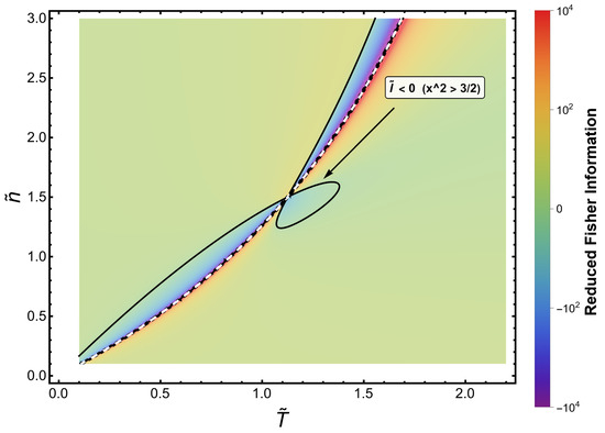
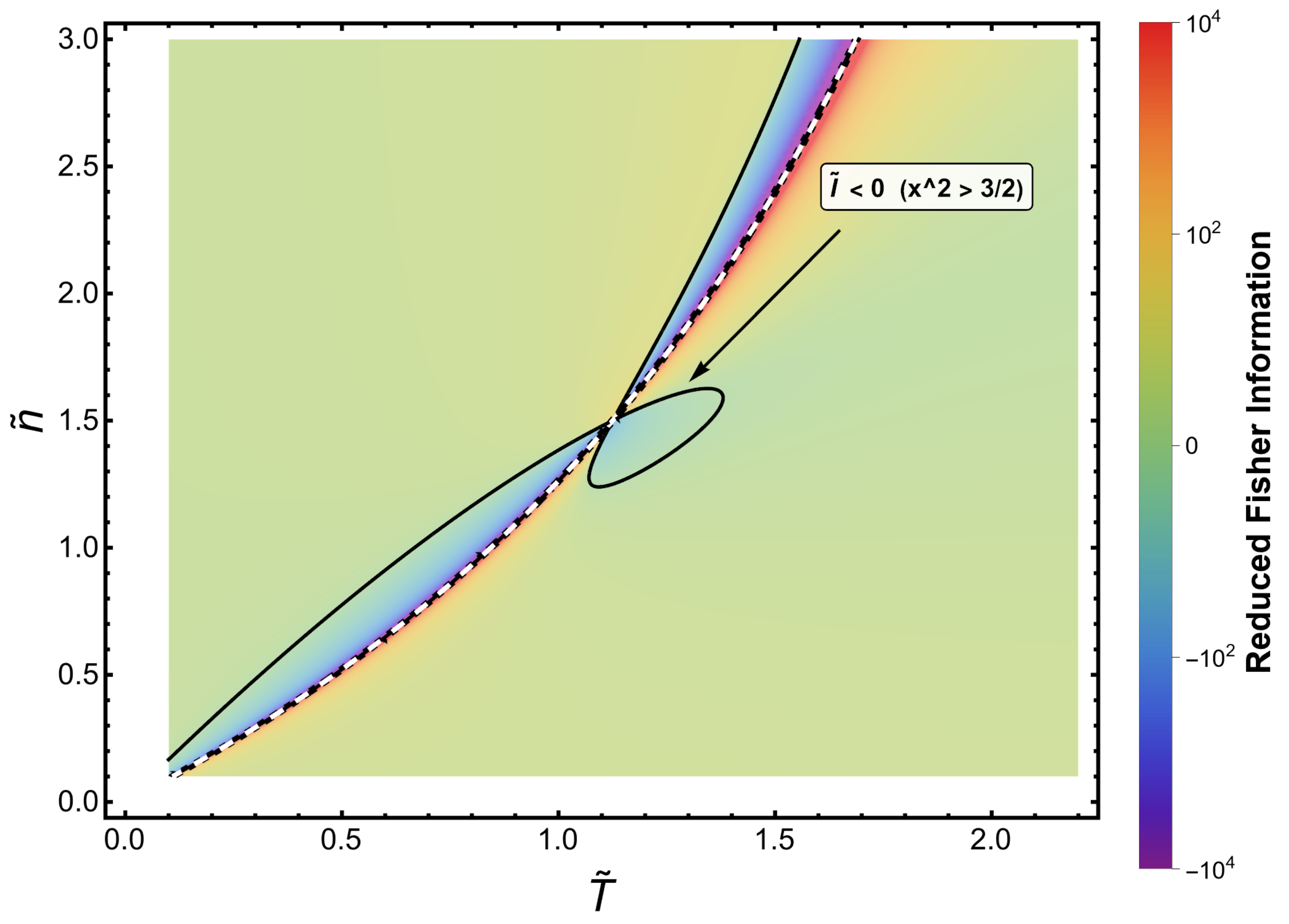
In Figure 1 we show the behaviour of the reduced Fisher information in the reduced density–temperature plane .
Figure 1.
Sign structure of the reduced Fisher information in the reduced density–temperature plane . The color map shows on a signed-log scale (green: , blue: ). The solid black curve is the zero contour , enclosing the pathological region where the mean-field closure causes the Fisher information to become negative (condition , or equivalently ). The dashed white curve denotes the closure boundary . Within the valid domain , the Fisher information is positive and provides a well-defined measure of energy fluctuations.
4.5. Reduced Heat Capacity and Fisher Information
The heat capacity at fixed fugacity is defined as
Using the relation between derivatives with respect to T and , one obtains
Recalling the definition of the Fisher information in Equation (30), we obtain the exact identity
Introducing the reduced heat capacity per particle,
where is the exact physical particle number [Equation (12)]—not itself—and using [Equation (31)] together with the normalized Fisher information , we obtain
Unlike the naive normalization by , Equation (48) shows that the reduced heat capacity per particle is not identical to the normalized Fisher information; the two differ by an explicit factor of the control parameter , reflecting the fact that n itself is not the physical density.
This modifies the critical scaling near the closure boundary. From Equation (32), the dominant singular contribution to as behaves as , so that . Combined with the extra factor of in Equation (48),
showing that the heat capacity per particle diverges at the closure boundary one power of more weakly than the Fisher information itself—a distinction that is invisible if is incorrectly identified with .
5. Hessian Structure
5.1. Hessian Determinant
We consider the Fisher measure within the present self-consistent closure, given by Equation (34). To analyze the geometry of the information surface, we define the Hessian determinant of the Fisher information in the space as
with .
After straightforward algebraic steps, the Hessian determinant can be written as
where [Equation (33)] and is the polynomial in x, given by
5.2. Reduced Dimensionless Hessian
Consistent with the reduced variables defined in Equation (36), we introduce the dimensionless Hessian . Substituting and , we obtain
with given by Equation (38), and the reduced polynomial is
where is the polynomial given in Equation (52).
Alternatively, absorbing the parameter-dependent prefactor into the definition of a dimensionless Hessian, we define
so that
The factor is the reduced form of the denominator controlling the isothermal response of the fluid within the present closure. Consequently, the Hessian exhibits singular behavior at , provided that the reduced polynomial does not cancel the corresponding leading divergence. Thus, the closure boundary discussed in Section 2 is a distinguished locus of the information-geometric Hessian.
5.3. Comments on the Hessian Structure
5.3.1. Sign Structure and Crossover Behavior
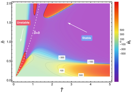
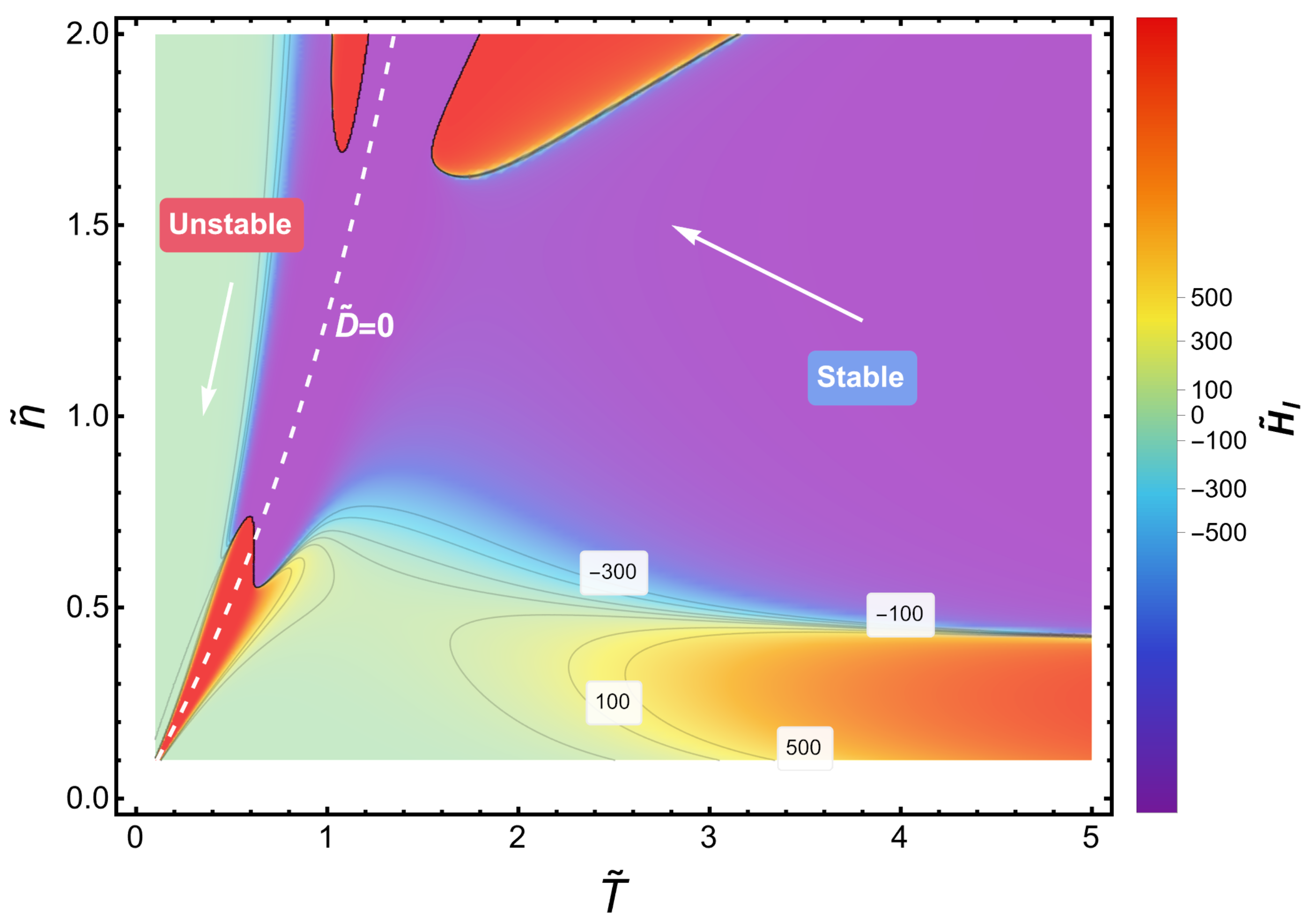
The polynomial is not sign-definite over the stable region : it changes sign along a well-defined contour , meaning likewise changes sign within the physically accessible domain. Consequently, Fisher-geometric crossover does occur with the corrected Fisher information and the natural coordinates . The locus (i.e., ) separates regions of saddle-like () and locally convex or concave () curvature of the Fisher information landscape. This sign change is a genuine feature of the geometry, not an artefact of the approximation; its structure is illustrated in Figure 2.
Figure 2.
Hessian determinant of the Fisher information in the reduced density–temperature plane . The color map encodes the value of : blue–purple tones indicate (saddle-like curvature), while green–yellow–red tones indicate . The two closed dark contours visible near and are the crossover loci (equivalently ), enclosing the regions where the curvature of the Fisher information landscape changes sign. The dashed white curve is the closure boundary , where diverges as . Labeled gray contours indicate selected values of , emphasizing the sharp growth near this boundary. The green region on the left is the mechanically unstable domain .
5.3.2. Critical Divergence
As , the Hessian exhibits a power-law divergence
reflecting the extreme sensitivity of the Hessian to the closure boundary discussed in Section 2: as , the response functions built from become singular and the self-consistent map between the closure parameter n and the physical density loses regularity.
The only singular behavior arises at this closure boundary, where the present mean-field description itself breaks down. In Figure 2 we display the behaviour of the Hessian determinant in the parameter space.
6. Ricci Scalar Curvature
6.1. Fisher Metric and Curvature
The Hessian of the logarithm of the grand partition function defines a natural symmetric bilinear form in parameter space,
where is the probability distribution in the grand canonical ensemble, and , with , are the natural exponential-family coordinates conjugate to and N, respectively. Within the domain where this Hessian is positive definite, it defines a genuine Fisher–Rao metric, providing a geometric measure of thermodynamic fluctuations and allowing the construction of the associated scalar curvature R [2,5,6]. As shown in Appendix A, because of the self-consistent mean-field closure of Section 2, is not guaranteed to remain the cumulant-generating function of an actual joint probability distribution of ; outside the region of positive-definiteness identified below, is only an indefinite Hessian extension, not a genuine Fisher–Rao metric.
6.2. Scalar Curvature Within the Present Closure
For the van der Waals form of the second virial coefficient, within the present self-consistent closure, explicit calculation (Appendix A) shows that the scalar curvature associated with the Fisher–Rao metric takes the closed form
with D given by Equation (33).
This structure shows that the scalar curvature inherits the same control parameter D governing thermodynamic stability. In particular, as , the curvature diverges as a simple pole,
reflecting the amplification of thermodynamic fluctuations near the closure boundary. Remarkably, this leading singular term is universal, independent of the interaction parameters ; interactions enter only through the subleading, regular terms above (see Appendix A for the full derivation, the resulting sign structure, and the domain of validity of the metric).
The pole is a formal singularity of the analytic continuation of the curvature expression. It is not accessible within the positive-definite Fisher–Rao domain, because the metric loses positive definiteness first at (Appendix A), well before the closure boundary is reached. There are thus two distinct singular loci in this problem: the formal closure boundary , and the physical Fisher-metric boundary , and the latter is always encountered first within the admissible Riemannian domain.
This result reinforces the central role of the control function D, which consistently governs the singular behavior of thermodynamic response functions, Fisher information, and the underlying information geometry.
6.3. Reduced Scalar Curvature: Closed Form
To maintain consistency with the dimensionless formulation introduced in the previous sections, we define the reduced scalar curvature
using a single power of , rather than the ansatz suggested by naive power counting.
Using the reference-scale definitions of Equation (35), the dimensionless combination appearing in the exact curvature of Equation (A11) reduces to
while the control function becomes , given in Equation (38). Substituting Equations (62) and (38) into Equation (A11), the V- and -dependence cancels identically, and one obtains the fully dimensionless closed form
This exact result (Appendix A) replaces the naive scaling estimate obtained from power counting on the self-consistent density equation (): an algebraic cancellation between the numerator and , invisible at the level of power counting, reduces the true divergence at the closure boundary to a simple pole,
i.e., the exponent in the general ansatz is , and the corresponding row of Table 1 should be read accordingly. Consequently, the scalar curvature diverges one power of more slowly than the Fisher information, versus : Fisher-geometric distinguishability and thermodynamic response are governed by different critical exponents near this boundary.
Table 1.
Unified role of the function in the thermodynamic and information-geometric description of the system.
As discussed in Appendix A, Equation (63) defines a genuine Riemannian curvature only where the Fisher–Rao metric remains positive-definite, i.e., for . In reduced variables this condition reads
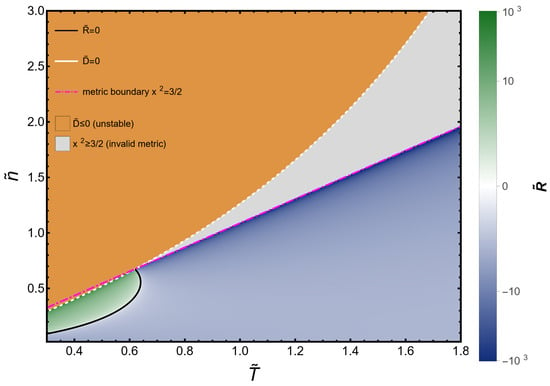
which lies strictly inside the mechanically stable region for all shown in Figure 3. The simple pole at implied by Equation (A12) is therefore never reached without first crossing the signature-changing locus (65); within the admissible domain , the dominant singular behavior of is instead governed by the vanishing of as , where . Figure 3 shows over the full plane, together with the closure boundary , the metric boundary , and the interior sign-change contour : within the admissible domain, the curvature is negative except in a pocket of strong effective coupling at low and low , where it turns positive before diverging on approach to the metric boundary.
Figure 3.
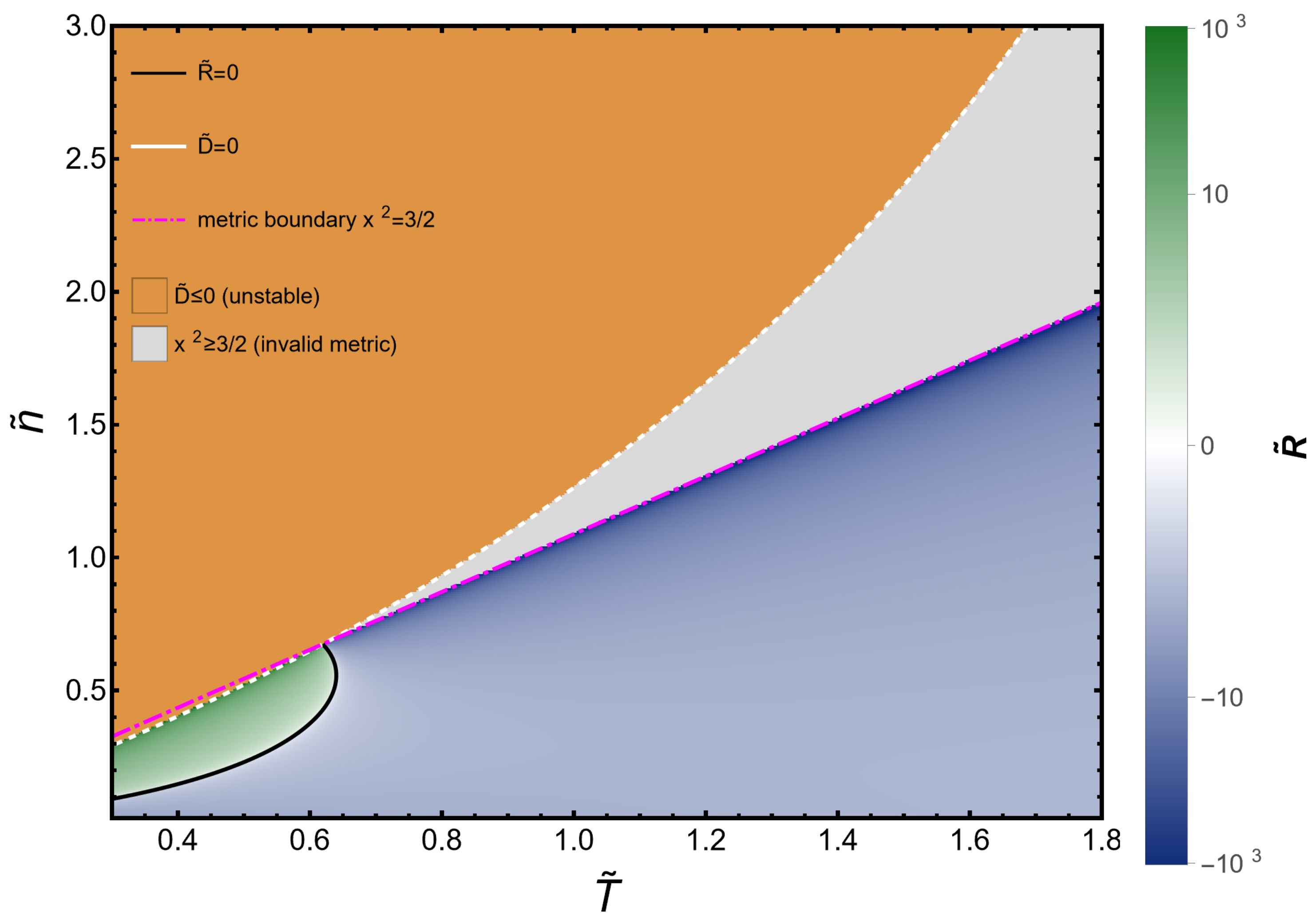
Reduced Fisher–Rao scalar curvature in the reduced density–temperature plane , Equation (63). The color map shows on a signed-log scale (green: , blue: ). The solid black curve is the interior zero contour , enclosing a pocket of positive curvature at low and low (strong effective coupling ); outside this pocket the curvature is negative and diverges on approach to the magenta dash-dotted curve. The magenta dash-dotted curve marks the metric boundary , Equation (65), beyond which the Fisher–Rao metric loses positive-definiteness (gray region); this is the dominant source of divergence of in the physically admissible domain. The dashed white curve is the closure boundary , where the leading term would formally diverge as a simple pole; this boundary lies outside the admissible domain (green region, , mechanically unstable) and is never reached without first crossing the metric boundary.
We plot in Figure 3 the reduced Fisher–Rao scalar curvature in the reduced density–temperature plane .
7. Summary of Main Results
Table 1 summarizes the central result of this work, highlighting how the control function governs the singular behavior across different physical layers.
While the equation of state carries no singular dependence on , response functions and information-geometric quantities exhibit singular inverse powers of , revealing a hierarchy of sensitivity to the closure boundary discussed in Section 2. Notably, the Ricci curvature diverges with the same exponent as the compressibility (), one power weaker than the heat capacity () and two powers weaker than the Fisher information (), showing that Fisher-geometric distinguishability and thermodynamic response are governed by distinct critical exponents (see Appendix A). We stress that the exponents associated with and describe the formal asymptotics of the corresponding closed-form expressions; the scalar curvature, in particular, loses its Riemannian meaning before this limit is reached, at the metric boundary (Section 6, Appendix A).
8. Conclusions
We have analyzed the information-geometric structure of a self-consistent second-virial approximation with the van der Waals form of the second virial coefficient, using the Fisher information as a generating potential. By constructing the associated Hessian metric and scalar curvature, we obtained a geometric characterization of thermodynamic fluctuations that complements the standard description based on macroscopic observables. Our results reveal three main features: First, interaction effects enter the Fisher information selectively through their temperature dependence. In particular, the attractive parameter a contributes via its thermal derivatives, while the excluded-volume parameter b enters primarily through the self-consistent control parameter D, whereas the explicitly interaction-sensitive derivative contribution is governed by the attractive parameter a. This shows that Fisher geometry probes the thermal responsiveness of interactions rather than their static magnitude. Second, the Hessian determinant of the Fisher information exhibits a rich sign structure in the reduced parameter space, changing sign along well-defined crossover loci that separate regions of saddle-like () and locally convex () curvature of the fluctuation landscape. Both the crossover loci and the divergence at the closure boundary are encoded in the polynomial of Equation (52). Third, an explicit closed-form calculation of the scalar curvature (Appendix A) shows that it diverges at the closure boundary as a simple pole, —one power of D weaker than the heat capacity, , and dramatically weaker than the Hessian determinant, —with a leading singular term that is universal and independent of the interaction parameters. This pole is, however, a formal singularity of the analytic continuation of R: within the physically admissible, positive-definite Fisher–Rao domain, the metric loses positive definiteness at , strictly before the closure boundary is reached. This closed-form result also shows that the curvature is not sign-definite: it is negative in the weakly-interacting regime but turns positive in the strong-coupling regime, at low reduced temperature and density (Figure 3), before diverging as the underlying Fisher–Rao metric itself loses positive-definiteness once the interaction is strong enough, restricting the hyperbolic-manifold picture to the corresponding region of parameter space (see Appendix A for the precise condition). This metric boundary lies strictly inside the mechanically stable region: the formal simple pole of the curvature at the closure boundary, , is therefore never reached in the physically admissible domain without first crossing it. The underlying algebraic mechanism is nonetheless shared with the Hessian determinant, whose divergence at the closure boundary follows from the same control parameter D, albeit with a different critical exponent. This divergence reflects the same sign change in mechanical stability discussed above, now propagating into the information-geometric quantities built from D. Taken together, these results indicate that Fisher geometry provides a physically meaningful probe of interacting systems at the level of fluctuations. Rather than signaling phase transitions through geometric singularities in the present approximation, it captures how interactions continuously reshape the distinguishability structure of thermal states. Future work should extend this analysis beyond the second virial approximation, where stronger correlations may induce genuinely nontrivial geometric features. It would also be of interest to compare Fisher and Ruppeiner geometries in regimes closer to criticality, as well as to explore quantum and nonequilibrium extensions, where information geometry may reveal qualitatively new behavior.
Author Contributions
The two authors have contributed in equal measure to the preparation of this manuscript. Investigation, F.P. and A.P.; Project administration, F.P. and A.P.; Writing—original draft preparation, F.P. and A.P. All authors have read and agreed to the published version of the manuscript.
Funding
Research was partially supported by ANID/FONDECYT, grant 1251928.
Data Availability Statement
No new data were created in this study. All derivations and results are presented within the article.
Conflicts of Interest
The authors declare no conflict of interest.
Appendix A. Explicit Calculation of the Fisher–Rao Scalar Curvature
In this appendix we carry out the calculation of the Ricci scalar curvature R of the Fisher–Rao metric explicitly, without resorting to power counting. The result corrects the scaling estimate quoted in the main text: the actual divergence at the closure boundary is .
Appendix A.1. Setup
We work with the natural exponential-family coordinates , , for which
with determined implicitly by
The Fisher–Rao metric is
Throughout, we use the control function D defined in Equation (33), and the dimensionless combination
Appendix A.2. A Useful Identity for Hessian Metrics
Because is itself the Hessian of a scalar potential (), the third partial derivatives are totally symmetric in all three indices. The Christoffel symbols of the first kind,
therefore collapse to
This identity (standard in the theory of Hessian/affine manifolds) considerably simplifies the construction of the Riemann tensor, since every geometric object is built directly out of derivatives of .
Appendix A.3. Derivatives of N(β,γ)
Implicit differentiation of Equation (A2) gives, to first order,
Differentiating again (all derivatives below are exact, obtained by repeated implicit/chain-rule differentiation and cross-checked by computer algebra)
Third derivatives are obtained in the same way (the algebra is straightforward but lengthy; we used computer algebra to carry it out and to verify all intermediate symmetry relations, e.g., ).
Appendix A.4. Closed-Form Scalar Curvature
Assembling and into Equation (A6), constructing the Riemann tensor, and contracting to the Ricci scalar, one obtains the exact closed-form result
This expression reduces to the flat result in the ideal-gas limit .
Appendix A.5. Divergence at the Closure Boundary: K=1
Equation (A11) is manifestly exact in D—it is not a truncated expansion. It shows that R has a simple pole at
with the remarkable feature that the leading singular term is universal: at leading order it does not depend on the interaction parameters at all. Interactions enter only through the sub-leading, finite terms in Equation (A11).
Appendix A.6. Corollary: Sign of the Divergence
Appendix A.7. Domain of Validity: Loss of Positive-Definiteness
Equation (A11) makes it natural to ask where the metric itself remains Riemannian. A direct computation gives the exact closed form
so that, since throughout the stable region, the metric is positive-definite if and only if
For the signature becomes indefinite (Lorentzian) and no longer defines a genuine Fisher–Rao metric. Crucially, the locus lies inside the mechanically stable region (): numerically, for representative parameters ( in the units of Section 2) the signature changes already at , well before the closure boundary . This is also visible directly in Equation (A11): the terms and diverge on the very same locus, so the sign change of R noted in the previous subsection and the loss of positive-definiteness are the same phenomenon, not two independent effects.
Physically, this is plausibly a consequence of the self-consistent mean-field closure of Equations (5)–(8): replacing inside the configurational integral before completing the grand-canonical sum means is no longer guaranteed to be the exact cumulant-generating function of a genuine joint distribution of . For an exact cumulant-generating function, the Cauchy–Schwarz inequality forces , i.e., automatically; the closure used here provides no such guarantee, and Equation (A14) shows explicitly that the guarantee indeed fails once interactions are strong enough.
We therefore recommend restricting the quantitative claims of Section 6 and Section 7 (in particular “negative throughout the stable domain” and the hyperbolic-manifold interpretation) to the region , and stating Equation (A15) explicitly as the actual domain of validity of the Fisher-geometric picture, rather than the full mechanically stable region .
References
- Rao, C.R. Information and the accuracy attainable in the estimation of statistical parameters. Bull. Calcutta Math. Soc. 1945, 37, 81–89. [Google Scholar]
- Amari, S.; Nagaoka, H. Methods of Information Geometry; American Mathematical Society: Providence, RI, USA, 2000. [Google Scholar]
- Weinhold, F. Metric geometry of equilibrium thermodynamics. J. Chem. Phys. 1975, 63, 2479–2483. [Google Scholar] [CrossRef] [Scilit]
- Ruppeiner, G. Thermodynamics: A Riemannian geometric model. Phys. Rev. A 1979, 20, 1608. [Google Scholar] [CrossRef] [Scilit]
- Ruppeiner, G. Riemannian geometry in thermodynamic fluctuation theory. Rev. Mod. Phys. 1995, 67, 605, Erratum in Rev. Mod. Phys. 1996, 68, 313. [Google Scholar] [CrossRef] [Scilit]
- Ruppeiner, G. Thermodynamic curvature measures interactions. Am. J. Phys. 2010, 78, 1170–1180. [Google Scholar] [CrossRef] [Scilit]
- Mandelbrot, B. Information theory and statistical mechanics. IRE Trans. Inf. Theory 1956, 2, 190. [Google Scholar]
- Crooks, G.E. Measuring thermodynamic length. Phys. Rev. Lett. 2007, 99, 100602. [Google Scholar] [CrossRef] [Scilit] [PubMed]
- Sivak, D.A.; Crooks, G.E. Thermodynamic metrics and optimal paths. Phys. Rev. Lett. 2012, 108, 190602. [Google Scholar] [CrossRef] [Scilit] [PubMed]
- Van der Waals, J.D. The Equation of State for Gases and Liquids. Nobel Lecture, 12 December 1910. In Nobel Lectures, Physics 1901–1921; Elsevier: Amsterdam, The Netherlands, 1967. [Google Scholar]
- Kittel, C.; Kroemer, H. Thermal Physics, 2nd ed.; Freeman: New York, NY, USA, 1980. [Google Scholar]
- Johnston, D.C. Advances in Thermodynamics of the van der Waals Fluid; Morgan and Claypool Publishers: San Rafael, CA, USA, 2014. [Google Scholar]
- De Boer, J. Van der Waals in his time and the present revival. Physica 1974, 73, 1–27. [Google Scholar] [CrossRef] [Scilit]
- Pennini, F.; Plastino, A. The Classical-Quantum Passage: A van der Waals Description. Entropy 2022, 24, 182. [Google Scholar] [CrossRef] [Scilit] [PubMed]
- Pathria, R.K.; Beale, P.D. Statistical Mechanics, 4th ed.; Academic Press: Cambridge, MA, USA, 2021. [Google Scholar]
- Pennini, F.; Plastino, A. An Endogenous Quantum–Classical Crossover Temperature in the van der Waals Fluid: Quantumness as an Emergent Behavior. Entropy 2026, 28, 789. [Google Scholar] [CrossRef] [Scilit] [PubMed]
- Reif, F. Fundamentals of Statistical and Thermal Physics, 1st ed.; Waveland Press: Long Grove, IL, USA, 2009. [Google Scholar]
- Callen, H.B. Thermodynamics and an Introduction to Thermostatistics, 2nd ed.; Wiley: New York, NY, USA, 1985. [Google Scholar]
- Frieden, B.R. Science from Fisher Information: A unification; Cambridge University Press: Cambridge, UK, 2004. [Google Scholar]
- Pennini, F.; Plastino, A. Analytical Information Links Between Fisher’s Measure and Gibbs’ Ensembles. Int. J. Catal. Chem. Eng. 2025, 1, 1–14. [Google Scholar]

Disclaimer/Publisher’s Note: The statements, opinions and data contained in all publications are solely those of the individual author(s) and contributor(s) and not of MDPI and/or the editor(s). MDPI and/or the editor(s) disclaim responsibility for any injury to people or property resulting from any ideas, methods, instructions or products referred to in the content. |
© 2026 by the authors. Licensee MDPI, Basel, Switzerland. This article is an open access article distributed under the terms and conditions of the Creative Commons Attribution (CC BY) license.