


Abstract
This study investigates software-based compensation of systematic indication errors in a precision Length Metroscope over the measurement range from 1.005 mm to 25 mm. Calibration was performed using 28 reference lengths represented by Grade 1 ceramic gauge blocks, with ten repeated measurements at each calibration point. The initial indication error ranged from 1.49 µm to 4.29 µm, and only 3.6 % of the investigated calibration points had mean indication errors numerically within the nominal ±1.5 µm MPE limits. Five compensation approaches were developed and compared: linear regression, third-order polynomial regression, piecewise linear interpolation, shape-preserving cubic Hermite interpolation (PCHIP), and Gaussian Process Regression (GPR). Predictive performance was evaluated using leave-one-out cross-validation. All methods reduced the original RMSE by more than 80 %. GPR achieved the lowest MAE of 0.287 µm and maximum residual of 0.737 µm, while linear regression provided an almost identical RMSE of 0.379 µm with substantially lower implementation complexity. The results demonstrate that software-based correction can significantly improve the effective metrological performance of existing precision length measuring instruments without mechanical modification.
1. Introduction
Dimensional metrology is a fundamental component of modern manufacturing and quality assurance because dimensional conformity directly influences product interchangeability, assembly capability, functional performance, and process control. Increasing requirements for manufacturing accuracy have simultaneously increased the demands placed on dimensional measuring equipment, particularly with respect to traceability, stability, measurement uncertainty, and conformity with specified metrological characteristics. Within the Geometrical Product Specifications (GPS) framework, measuring equipment must be characterized by clearly defined metrological properties, while dimensional measurements are referred to a standard reference temperature of 20 °C [1,2]. At the same time, reliable interpretation of calibration and verification results requires a consistent treatment of measurement uncertainty and conformity decisions, particularly when measured deviations approach the maximum permissible error (MPE) of an instrument [3,4,5,6,7].
Precision length measurement relies on traceable reference standards capable of transferring the realization of the unit of length from primary standards to industrial measuring equipment. Gauge blocks remain among the most important material length standards for this purpose. Their dimensional and metrological characteristics are standardized by ISO 3650, and their calibration may be performed either by interferometric methods or by mechanical comparison against reference gauge blocks of higher metrological quality [8,9]. Considerable research has therefore been devoted to improving gauge-block calibration and evaluating its associated uncertainty. Interferometric investigations have addressed wavelength realization, phase correction, thermal effects, wringing, optical imperfections, and the calibration of both short and long gauge blocks [9,10,11,12,13,14,15]. Mechanical comparison methods have likewise been investigated with particular attention to uncertainty budgets, comparator behaviour, repeatability, and traceability transfer [16,17]. More recent developments include automated interferometric systems and international comparisons of short gauge blocks, demonstrating the continuing importance of reliable material length standards in dimensional metrology [18,19].
The calibration of dimensional measuring instruments, however, is not limited to establishing the properties of the reference standards themselves. The complete measurement chain must be characterized, including the displacement transducer, mechanical guide system, measuring contacts, positioning mechanism, environmental influences, data acquisition system, and numerical processing of the measurement result. Modern calibration systems therefore increasingly combine material standards with interferometric or encoder-based reference systems. Step gauges, precision positioning stages, and optical linear encoders have been investigated as transfer standards or displacement-measurement systems for high-accuracy dimensional calibration [20,21,22,23,24]. These studies demonstrate that even high-resolution measuring systems can exhibit position-dependent, cyclic, thermal, geometric, or interpolation errors and that the nominal resolution of a measuring system alone cannot be regarded as an indicator of its achievable measurement accuracy.
In precision length measuring equipment, the observed indication error generally results from the combined action of systematic and random influences. Geometric imperfections of guideways, scale errors, positioning errors, Abbe offsets, angular motions, elastic deformation, contact conditions, thermal expansion, encoder interpolation errors, and assembly deviations can produce a position-dependent error characteristic. When these influences remain sufficiently stable, a substantial part of the resulting deviation is systematic and therefore potentially correctable. This principle has been extensively investigated in machine-tool and coordinate-metrology research. Early studies established mathematical approaches for geometric-error identification and numerical compensation [25], while subsequent work demonstrated increasingly comprehensive strategies for mapping, modelling, and correcting position-dependent and volumetric errors [26,27,28,29,30,31,32,33,34,35,36,37,38]. The development of numerical compensation has consequently transformed calibration data from a purely diagnostic result into information that can also be used to improve the effective accuracy of a measuring or positioning system.
Software-based error compensation is particularly attractive for existing precision instruments because it can improve their effective metrological performance without mechanically rebuilding the measuring structure. In its simplest form, compensation may be based on a global analytical model, such as linear or polynomial regression, where a single mathematical function describes the error over the entire measuring range. Such models require only a small number of coefficients and are readily implemented in measurement software or embedded controllers. Alternatively, local approaches based on correction tables and interpolation can reproduce position-dependent deviations more closely because the correction at a given location is determined from neighbouring calibration points. Piecewise linear interpolation provides a computationally simple implementation, whereas higher-order interpolation can produce smoother correction functions. Error maps, lookup tables, regression models, and local correction strategies have all been successfully applied in precision positioning, machine-tool calibration, and coordinate metrology [25,26,27,28,29,30,31,32,33,34,35,36,37,38,39,40,41]. Nevertheless, the choice of model involves an inherent trade-off between numerical complexity, local adaptability, robustness, and predictive capability.
An important limitation of highly flexible compensation functions is that close reproduction of the calibration points does not necessarily imply equally good prediction at positions that were not explicitly used to construct the model. A local interpolation function can reproduce an experimental calibration curve almost exactly and yet remain sensitive to local measurement fluctuations, point spacing, or extrapolation at the boundaries. Conversely, a low-order global approximation may suppress local variations but provide greater robustness when the dominant systematic component follows a relatively smooth trend. The distinction between fitting accuracy and predictive performance is therefore particularly important when compensation models are intended for practical measurement rather than only for retrospective description of calibration data. Contemporary machine-tool calibration research similarly emphasizes the need to consider model identification, validation, uncertainty, and robustness rather than approximation accuracy alone [29,30,31,32,33,34,35,36,37,38].
The increasing digitalization of measurement systems has also stimulated the application of data-driven modelling techniques for systematic-error prediction. In machine-tool metrology, statistical learning and artificial-intelligence methods have been used extensively for thermal-error compensation, where the relationship between temperature, machine state, and geometric deviation is frequently nonlinear and time-dependent. Approaches based on principal-component regression, adaptive neuro-fuzzy inference systems, least-squares support vector machines, adaptive input selection, recurrent neural networks, and self-optimizing autoregressive models have demonstrated that data-driven methods can provide effective correction when conventional analytical models are insufficient [42,43,44,45,46,47,48,49,50,51,52]. Recent investigations have further integrated uncertainty analysis, digital-twin concepts, optimized sensor information, and adaptive model updating into error compensation, indicating a transition from static calibration tables toward information-rich and potentially self-adaptive correction systems [53,54,55]. Recent studies demonstrate a continued evolution toward more adaptive machine learning architectures, uncertainty-aware compensation, and model updating under changing operating conditions [55,56,57].
Among probabilistic regression techniques, Gaussian Process Regression (GPR) is particularly relevant to calibration problems involving relatively small experimental datasets. A Gaussian process defines a probability distribution over possible functions and uses the covariance between observations to infer the response at unmeasured positions. Unlike a fixed-order polynomial, the shape of the regression function is therefore determined by the data and the selected covariance kernel rather than by a predefined algebraic equation. GPR additionally provides a probabilistic description of its predictions, which is attractive for metrological applications in which prediction reliability is of interest. The fundamental formulation of Gaussian processes for nonlinear regression was established by Williams and Rasmussen [49]. More recently, Wei et al. applied GPR to thermal-error modelling and compensation of CNC machine tools and demonstrated its suitability for describing complex systematic-error behaviour [50].
Despite the extensive development of geometric, thermal, and volumetric compensation methods, the existing literature is dominated by machine tools, coordinate measuring machines, precision positioning stages, and encoder systems [20,21,22,23,24,25,26,27,28,29,30,31,32,33,34,35,36,37,38,39,40,41,42,43,44,45,46,47,48,49,50,51,52]. Comparatively less attention has been devoted to the direct comparison of multiple compensation strategies for conventional precision length measuring instruments operating over short measurement ranges. There remains a practical need to determine whether the added complexity of nonlinear interpolation or probabilistic machine learning models provides a meaningful improvement over simple global regression when the instrument exhibits a predominantly systematic length-dependent error. The surveyed literature also indicates that methods are often evaluated under different instruments, datasets, operating conditions, and performance criteria, which complicates direct comparison of their effectiveness. This motivates the use of one common experimental dataset and one common validation procedure for all investigated compensation approaches. This research-gap statement is an inference from the distribution of applications in the cited literature.
A further methodological consideration concerns the distinction between calibration-model fitting and actual compensation capability. If a model is evaluated only using the same calibration points from which it was constructed, highly flexible interpolation techniques can produce artificially small residuals. Independent validation is therefore required to assess whether the identified systematic relationship is sufficiently stable to predict an omitted calibration point. For a limited number of calibration positions, leave-one-out cross-validation (LOOCV) offers a suitable strategy because each observation is successively treated as an independent validation point while the remaining observations are used for model construction. Such an approach enables the compensation methods to be compared under identical experimental conditions and prevents the assessment from being based exclusively on in-sample fitting quality.
Based on the identified research gap, the present study investigates the calibration and software-based compensation of a precision Length Metroscope over the range from 1.005 mm to 25 mm. Twenty-eight reference lengths represented by Grade 1 ceramic gauge blocks were investigated, with ten repeated measurements performed at each calibration point. The initial calibration was used to characterize the systematic indication error and its repeatability relative to the specified MPE of ±1.5 μm. The same experimental dataset was subsequently used to develop five compensation approaches: linear regression, third-order polynomial regression, piecewise linear interpolation, shape-preserving piecewise cubic Hermite interpolation (PCHIP), and Gaussian Process Regression with a squared-exponential covariance function.
Accordingly, the objectives of this study are: (1) to experimentally characterize the indication-error behaviour and repeatability of the investigated Length Metroscope over the calibrated range; (2) to develop compensation models representing global regression, local interpolation, and probabilistic data-driven approaches; (3) to evaluate their predictive capability using an identical leave-one-out cross-validation procedure; and (4) to compare the models using the root mean square error (RMSE), mean absolute error (MAE), maximum absolute residual error, cross-validated coefficient of determination, and the percentage of cross-validated residuals falling within a ±1.5 µm residual benchmark corresponding numerically to the nominal MPE magnitude.
The principal contribution of the work is therefore not limited to obtaining a calibration equation for one measuring instrument. Instead, the study establishes a common experimental framework for the direct comparison of compensation methods with substantially different mathematical complexity. Three main contributions are provided: (1) experimental characterization of a precision Length Metroscope using 280 repeated measurements distributed across 28 reference lengths; (2) a direct comparison of classical global and local correction techniques with GPR using identical calibration data and validation conditions; and (3) an assessment of the trade-off between predictive accuracy and implementation complexity, providing a basis for selecting a compensation strategy for existing precision dimensional measuring equipment.
The remainder of the paper is organized as follows. Section 2 describes the Length Metroscope, reference standards, environmental conditions, calibration procedure, mathematical compensation models, and validation criteria. Section 3 presents the experimental calibration results and the performance of the investigated compensation methods. Section 4 discusses the results from both metrological and practical implementation perspectives, including the relative advantages of simple regression and data-driven compensation. Finally, Section 5 summarizes the main conclusions and outlines directions for further experimental validation and uncertainty-aware compensation.
2. Materials and Methods
The experimental study was designed to characterize the systematic indication error of a precision Length Metroscope and to obtain a consistent dataset for the subsequent development and comparison of mathematical compensation models. The experimental procedure included characterization of the investigated measuring instrument, selection of traceable reference standards, control of environmental conditions, repeated measurements at individual calibration points, and statistical evaluation of the obtained results.
The investigated range extended from 1.005 mm to 25 mm, corresponding to the physical working displacement of the measuring mechanism, and consisted of 28 reference lengths distributed across the complete stroke. Each reference length was measured ten times, resulting in a total of 280 individual measurements. The resulting calibration dataset was subsequently used for error modelling, compensation, and cross-validated comparison of the investigated correction methods.
2.1. Length Metroscope
The investigated instrument was a precision Length Metroscope intended for comparative dimensional measurements over short measuring ranges. The instrument consists of a rigid mechanical frame, fixed and movable measuring contacts, a precision displacement mechanism, and an indication system used to determine the displacement corresponding to the measured length.
During measurement, the reference standard is positioned between the measuring contacts. The movable measuring contact is displaced until contact with the opposite measuring surface is established, after which the instrument indication is recorded and compared with the corresponding certified reference value.
The Length Metroscope used in the experimental investigation is shown in Figure 1.
Figure 1.
Precision Length Metroscope used in the calibration experiment.
According to the specified metrological characteristics of the investigated instrument, the maximum permissible error within the evaluated range is MPE = ±1.5 µm. The digital resolution of the indication system was 0.0001 mm (0.1 µm).
No mechanical adjustment, correction, or modification of the Length Metroscope was performed before calibration. This was intentional because the objective was first to characterize the actual metrological condition of the instrument and subsequently to investigate whether the observed systematic indication error could be reduced by mathematical software-based compensation.
The physical working displacement of the investigated Length Metroscope is approximately 0 mm–25 mm. Although the instrument allows measurements of larger nominal dimensions, up to approximately 100 mm, these extended ranges are obtained through a scaling coefficient in the indication system, while the underlying mechanical measuring displacement remains within the same 0 mm–25 mm stroke. Because the present study focuses on position-dependent systematic errors associated with the physical displacement of the measuring mechanism, the calibration and compensation analysis was restricted to the interval from 1.005 mm to 25 mm. Accordingly, the developed compensation models and the conclusions concerning their performance are valid only for this experimentally investigated physical displacement range. Extended nominal measurement ranges were not evaluated in the present study and would require separate verification before application of the proposed compensation.
2.2. Reference Standards
Calibration was performed using a set of Grade 1 ceramic gauge blocks. Gauge blocks are widely used as material length standards in dimensional metrology and provide a direct means of transferring metrological traceability to precision measuring instruments. Their dimensional and metrological requirements are specified in ISO 3650 [8].
Ceramic gauge blocks were selected because of their dimensional stability, high wear resistance, corrosion resistance, and suitability for repeated contact measurements. The selected standards covered the investigated dimensional interval and provided reference lengths distributed throughout the entire calibration range.
The gauge blocks used during the experimental calibration are shown in Figure 2.
Figure 2.
Grade 1 ceramic gauge blocks used as reference standards.
The reference value assigned to each gauge block was obtained from its calibration documentation. Therefore, the indication error of the Length Metroscope was evaluated using the certified reference length rather than only the nominal value marked on the gauge block.
The calibration documentation also provided the standard uncertainty of the reference gauge blocks. For gauge blocks within the range from 1.005 mm to 9 mm, the standard uncertainty was uref = 0.10 µm. For gauge blocks from 10 mm to 25 mm, the corresponding standard uncertainty was uref = 0.15 µm. These values were subsequently included directly in the uncertainty budget of the compensated measurement result.
For a gauge block having a nominal length Lnom,i and a certified deviation from nominal length ΔLGB,i, the reference length can be expressed as
where Lref,i is the calibrated reference value used at the i-th calibration point.
Lref,i = Lnom,i + ∆LGB,i,
The use of calibrated reference values ensures that the deviations of individual gauge blocks from their nominal dimensions are taken into account and provides metrological traceability of the experimental calibration results.
2.3. Environmental Conditions
Dimensional measurements are sensitive to temperature because both the measuring instrument and the reference standards are affected by thermal expansion. According to ISO 1, the standard reference temperature for dimensional and geometrical measurements is 20 °C [2].
Prior to the calibration experiment, the Length Metroscope and the ceramic gauge blocks were allowed to thermally stabilize under laboratory conditions. The temperature during calibration was maintained at 20 °C ± 1 °C. The standard uncertainty associated with temperature measurement was 0.01 °C. This contribution was subsequently propagated to the measured length through the thermal sensitivity coefficient and included in the uncertainty budget of the corrected measurement result.
The laboratory temperature was monitored during the experiment in order to minimize the influence of thermal variations on both the measuring instrument and the reference standards.
No deliberate variation in environmental conditions was introduced during the experiment. All calibration measurements were therefore performed under nominally comparable laboratory conditions so that the observed changes in indication error could primarily be associated with the metrological behaviour of the instrument rather than with intentionally varying environmental influences.
2.4. Calibration Procedure
The calibration procedure was designed to characterize both the overall trend and local variations in the indication error over the complete physical working stroke of the Length Metroscope. A total of 28 reference lengths between 1.005 mm and 25 mm were selected. The calibration positions were distributed across the entire investigated interval with a maximum spacing of 1 mm between neighbouring points; several additional points were included in the lower part of the range, where the spacing was reduced to 0.1 mm–0.5 mm. Considering the complete interval, the average spacing between adjacent calibration positions was approximately 0.89 mm. The number and distribution of calibration points were selected to provide sufficiently dense sampling of the physical displacement range to identify both the global systematic trend and local deviations of the indication error. At the same time, 28 calibration positions provided a dataset sufficiently large for direct comparison of compensation models with substantially different mathematical complexity. In each LOOCV iteration, 27 calibration points remained available for model construction. This number is substantially larger than the number of coefficients required by the linear and third-order polynomial regression models and also provides a relatively dense set of nodes for the interpolation-based and GPR approaches.
The selection of 28 points was therefore intended to provide a detailed characterization of the instrument over its physical working stroke rather than to establish a mathematically optimal number of calibration positions. Optimization of calibration-point density was outside the scope of the present study.
Before each measurement series, the measuring contacts of the Length Metroscope and the measuring surfaces of the corresponding gauge block were cleaned in order to minimize the influence of dust, grease, and other surface contamination. The gauge block was subsequently positioned between the measuring contacts and aligned with the measurement direction to reduce positioning and cosine errors.
Each reference length was measured ten times under nominally identical conditions. Between repeated measurements, the gauge block was repositioned so that the observed variation included not only the short-term variability of the indication system but also the influence associated with repeated positioning and establishment of the measuring contact.
For every calibration point, the arithmetic mean of the ten repeated measurements was calculated as
where is the mean indicated length at the i-th calibration point, Lind,ij is the j-th indication obtained at the i-th reference length, n = 10 is the number of repeated measurements.
The mean indication error at each calibration point was then determined as
where ei denotes the indication error and Lref,i is the certified reference length of the corresponding gauge block.
According to Equation (3), a positive value of ei indicates that the Length Metroscope overestimates the reference length, whereas a negative value of ei indicates underestimation.
The repeatability of the measurement process was characterized using the experimental standard deviation of the ten repeated measurements:
where si is the experimental standard deviation at the i-th calibration point.
The experimentally determined indication error was compared with the specified maximum permissible error of the instrument. For descriptive comparison with the nominal instrument specification, the mean indication error at each calibration point was compared with the numerical MPE limits of ±1.5 µm. A calibration point was classified as lying within the nominal MPE band when
|ei| ≤ 1.5 μm.
This classification is used only to describe the magnitude of the experimentally observed indication error relative to the nominal MPE limits and should not be interpreted as a formal conformity decision, which requires consideration of measurement uncertainty and an appropriate decision rule [5,6,7].
The final experimental dataset therefore consisted of 28 reference lengths, their corresponding mean indication errors, and the standard deviations calculated from ten repeated measurements at each calibration position. The complete experimental calibration results are summarized in Table 1.
Table 1.
Experimental calibration results of the investigated Length Metroscope.
The complete calibration dataset was subsequently used as the common input for all investigated mathematical compensation methods. Using identical experimental data for each model ensured that differences in predictive performance were attributable to the mathematical compensation strategy rather than to differences in the underlying calibration dataset.
2.5. Mathematical Compensation Models
The experimentally determined indication errors were used to construct mathematical models describing the systematic error of the Length Metroscope as a function of the measured length. The objective of the compensation procedure was to estimate the systematic component of the indication error and subsequently subtract this estimated error from the instrument indication. Similar numerical compensation strategies are widely applied in precision positioning systems, coordinate metrology, and machine-tool calibration [25,26,27,28,29,30,31,32,33,34,35,36,37,38].
Five compensation approaches with different levels of mathematical complexity were investigated:
- Linear regression;
- Third-order polynomial regression;
- Piecewise linear interpolation;
- Shape-preserving piecewise cubic Hermite interpolation (PCHIP);
- Gaussian Process Regression (GPR).
All models were developed using the same set of 28 calibration points so that their performance could be compared under identical experimental conditions.
Throughout the compensation analysis, all length quantities are expressed in millimetres, whereas indication errors, predicted errors, and residual errors are expressed in micrometres unless stated otherwise.
For the i-th calibration point, the experimentally determined mean indication error was denoted by ei, while the corresponding reference length was denoted by Li. Each compensation model provided an estimate of the systematic indication error:
where f(L) represents the mathematical compensation function and where L denotes the certified reference length during model identification and validation
The corrected indication can then be expressed as
where Lind is the original instrument indication expressed in millimetres, is the predicted systematic indication error expressed in micrometres, and Lcorr is the corrected measurement result expressed in millimetres. During model construction, the certified reference lengths were used as the independent variable. The same calibration dataset was used for all five models.
During calibration, Lref is known from the certified value of the corresponding gauge block and is therefore used as the independent variable of the compensation function. The same applies during LOOCV, where the omitted calibration position remains known and the model predicts the indication error at that reference length. In routine measurement, however, the true reference length is unknown. Therefore, the raw instrument indication Lind is used as an initial estimate of the position at which the compensation function is evaluated.
This substitution introduces only a very small difference in the model input because Lind − Lref corresponds to the indication error, which did not exceed 4.29 µm (0.00429 mm) in the present experiment. This displacement is substantially smaller than the spacing between neighbouring calibration points and is also small relative to the investigated measurement range. For practical implementation, the estimate can additionally be refined iteratively as described in Section 2.7.
2.5.1. Linear Regression
Linear regression was selected as the simplest global compensation model. It assumes that the systematic indication error changes approximately linearly with the measured length. The compensation function is defined as
where a0 is the intercept and a1 is the slope of the regression line.
The coefficients were determined by minimizing the sum of squared differences between the experimentally determined indication errors and the model predictions:
where N = 28 represents the number of calibration points.
Linear regression provides a computationally efficient correction model requiring only two coefficients. Its main advantage is straightforward implementation in measurement software or embedded systems. However, a single straight line cannot reproduce local nonlinear variations in the calibration curve. The model was therefore included both as a practical compensation method and as a baseline against which the more complex approaches could be compared.
2.5.2. Polynomial Regression
A third-order polynomial model was used to provide greater flexibility in representing nonlinear variations in the systematic error. The predicted indication error is expressed as
where b0, b1, b2, and b3 are regression coefficients obtained from the experimental calibration data.
The third-order polynomial was selected as a compromise between model flexibility and numerical complexity. Compared with linear regression, it is capable of reproducing gradual curvature in the error characteristic without requiring a large number of parameters.
Higher polynomial orders were not considered because increasing the polynomial degree can improve the approximation of the calibration points while simultaneously increasing sensitivity to local fluctuations and producing unrealistic behaviour between or outside the calibrated positions. This is particularly relevant for compensation models, where predictive performance is more important than exact reproduction of the calibration dataset.
Polynomial compensation has been widely employed in numerical correction of systematic machine and positioning errors because of its simple mathematical representation and low computational requirements [25,26,27,28,29,30].
2.5.3. Piecewise Linear Interpolation
In contrast to the global regression models, piecewise linear interpolation represents the calibration characteristic locally. The measured indication errors themselves form correction nodes, and the error between two adjacent calibration points is estimated by linear interpolation.
For a length L located between two neighbouring calibration points Li and Li+1,
the estimated error is calculated as
Li ≤ L ≤ Li+1,
This method exactly reproduces the experimental mean error at every calibration node and does not require the estimation of global regression coefficients.
From an implementation perspective, piecewise linear interpolation can be interpreted as a correction lookup table combined with linear interpolation between neighbouring entries. Such an approach is attractive for industrial measuring systems because of its simplicity and low computational demand.
However, exact reproduction of calibration points does not necessarily guarantee superior predictive performance. The method can be sensitive to local experimental fluctuations because each segment is directly determined by two neighbouring calibration values. Its behaviour at the boundaries of the calibrated range must also be considered when extrapolation is required.
2.5.4. Shape-Preserving Cubic Hermite Interpolation
To obtain a smoother local compensation function while limiting the oscillations that may occur with conventional cubic spline interpolation, shape-preserving piecewise cubic Hermite interpolation (PCHIP) was also investigated.
PCHIP constructs an individual cubic polynomial between each pair of neighbouring calibration points while preserving the local shape and monotonic behaviour of the data. For the interval between and, the interpolation can be written in the general Hermite form
where
and
hi = Li+1 − Li
The cubic Hermite basis functions are
and
h00(t) = 2t3 − 3t2 + 1,
h10(t) = t3 − 2t2 + t,
h01(t) = −2t3 + 3t2,
h11(t) = t3 − t2.
The quantities di and di+1 represent the local derivatives at Li and Li+1, respectively, determined from neighbouring calibration points using the shape-preserving interpolation algorithm.
Unlike a conventional cubic spline, PCHIP limits overshoot between adjacent data points and therefore provides a smoother representation of the calibration characteristic while preserving its local shape. This property makes it potentially suitable for compensation of systematic errors characterized by local variations.
At the same time, PCHIP remains fundamentally an interpolation-based model and consequently reproduces the calibration nodes exactly. Its behaviour is therefore most reliable when the evaluated position lies between two retained calibration nodes. Near the boundaries of the calibration interval, particular care is required. If a prediction is requested outside the outermost available calibration nodes, PCHIP no longer operates as an interpolation method but extrapolates the terminal cubic segment. In this situation, the predicted value is not constrained by calibration data on both sides of the evaluated position and can therefore become more sensitive to the local slope and curvature estimated at the boundary. For this reason, the predictive performance of PCHIP should be evaluated separately for internal and boundary positions, and extrapolation beyond the calibrated domain should be avoided in practical compensation.
2.5.5. Gaussian Process Regression
Gaussian Process Regression was investigated as a probabilistic data-driven alternative to conventional regression and interpolation methods. GPR is particularly suitable for relatively small datasets because it can represent nonlinear relationships without requiring a predefined polynomial form [49,50].
A Gaussian process defines a distribution over possible functions and is described by a mean function m(L) and a covariance function k(L, L′):
e(L) = GP[m(L), k(L, L′)].
In the present implementation, a constant basis function was used for the mean component, such that m(L) = β0, where β0 is estimated from the calibration data. The observed indication error was modelled as the sum of the latent Gaussian-process response and independent additive measurement noise:
where σn denotes the observation-noise standard deviation.
ei = f(Li) + εi,
In the present study, the relationship between the reference length and the systematic indication error was modelled using a squared-exponential covariance function
where represents the signal variance and l is the characteristic length scale controlling the smoothness of the predicted error function.
The measured calibration data can additionally contain random variability. Consequently, the covariance matrix of the observations can be expressed as
where K is the covariance matrix obtained from the squared-exponential kernel, is the variance of the independent Gaussian observation-noise term, and I is the identity matrix. The noise variance was not fixed a priori but was estimated from the calibration data during GPR fitting. For a new length L*, the predicted systematic indication error is obtained from the posterior mean of the Gaussian process:
where e contains the experimentally determined indication errors, k* represents the covariance between the new input and the calibration points, and m contains the corresponding values of the mean function.
The GPR model was implemented in MATLAB R2026a using the fitrgp function. The squared-exponential covariance function and a constant basis function were used. The predictor, corresponding to measurement length, was standardized by centering and scaling during model fitting (Standardize = true). Because the dataset contained only 28 observations, exact Gaussian-process fitting was used. The observation noise was assumed to be independent, additive, and normally distributed with zero mean. Its standard deviation σn was not fixed but was estimated during model fitting together with the kernel parameters and the constant mean coefficient by optimization of the Gaussian-process marginal likelihood. Parameter estimation was performed using the quasi-Newton optimization procedure. No separate external hyperparameter-search procedure was applied.
The equivalent MATLAB model specification can be expressed as fitrgp(L, e, ‘KernelFunction’, ‘squaredexponential’, ‘BasisFunction’, ‘constant’, ‘Standardize’, true, ‘FitMethod’, ‘exact’, ‘ConstantSigma’, false), with the remaining optimization settings retained at their MATLAB defaults.
Unlike conventional interpolation, GPR does not require the correction function to pass exactly through every calibration point. Instead, it balances agreement with the observed data against the smoothness implied by the covariance function. This characteristic can be advantageous when the calibration dataset contains both a systematic trend and random measurement variability.
An additional feature of GPR is the possibility of estimating the predictive standard deviation together with the predicted mean response. In MATLAB, the predict function was used to obtain both quantities. The returned predictive standard deviation describes the uncertainty of the predicted response and therefore includes the observation-noise component. For visualization of the GPR predictive dispersion, a nominal 95 % prediction interval was calculated as
where spred(L) is the predicted response standard deviation. This interval was used only to visualize the predictive dispersion of the fitted GPR model and was not used as a substitute for the complete measurement uncertainty evaluated in Section 2.8 [49,50].
The five investigated compensation models therefore represent different modelling philosophies. Linear and polynomial regression provide global analytical approximations; piecewise linear interpolation and PCHIP provide local data-driven correction functions; and GPR provides a probabilistic nonlinear regression model. Their performance cannot be evaluated solely from their ability to fit the original calibration points. Therefore, an identical cross-validation procedure was subsequently applied to all models, as described in Section 2.6.
2.6. Model Validation and Performance Metrics
The performance of the compensation models was evaluated using a common validation procedure to ensure a direct and unbiased comparison between methods with different levels of mathematical complexity. Evaluation based only on the same calibration points used for model construction would be insufficient, particularly for interpolation-based methods, because such models can reproduce the calibration data exactly while providing poorer predictions at unmeasured positions. Therefore, leave-one-out cross-validation (LOOCV) was applied to all five compensation models.
For a dataset containing calibration points, LOOCV consists of N = 28 consecutive validation steps. In each step, one calibration point was excluded from the dataset and treated as an independent validation point. The corresponding compensation model was then reconstructed using the remaining N − 1 = 27 calibration points, and the indication error at the omitted reference length was predicted.
For the i-th validation step, the predicted error can be expressed as
where f−i denotes the compensation model constructed without the i-th calibration point and is the predicted systematic error at the omitted reference length Li.
The corresponding cross-validated residual error was calculated as
where ei represents the experimentally determined mean indication error at the omitted calibration point.
The ri residual therefore represents the indication error that would remain after applying the compensation predicted from the remaining calibration data. A residual value close to zero indicates that the model is able to predict the systematic error accurately at a calibration position that was not used during model construction.
All investigated models were retrained independently during each cross-validation iteration. For linear and polynomial regression, new regression coefficients were determined from the remaining 27 calibration points. Piecewise linear interpolation and PCHIP were reconstructed from the reduced calibration dataset. Similarly, the GPR model was refitted during each iteration using only the corresponding training subset. This procedure prevented information from the validation point from influencing model construction.
For the interpolation-based methods, omission of an internal calibration point resulted in prediction by interpolation between the neighbouring retained calibration positions. Of the 28 LOOCV iterations, 26 involved omission of an internal calibration point and therefore remained genuine interpolation cases. The remaining two iterations corresponded to omission of the lower boundary point at 1.005 mm and the upper boundary point at 25 mm. In these two cases, the validation position lay outside the range defined by the remaining 27 calibration points and prediction necessarily required extrapolation. Consequently, boundary extrapolation occurred in
of the LOOCV iterations, whereas 92.9 % of the iterations remained within the interpolation domain. These endpoint cases were intentionally retained because excluding them would artificially improve the reported predictive performance of the interpolation-based methods and would provide an incomplete assessment of their behaviour near the limits of the calibrated range.
It should be noted that omission of an endpoint also places the validation input outside the reduced training-input interval for the global regression and GPR models. However, the term boundary extrapolation is used here specifically in relation to the interpolation-based methods, for which omission of an endpoint changes the mathematical operation from interpolation between neighbouring nodes to extrapolation of the terminal segment.
This distinction is particularly important for PCHIP. For an omitted internal calibration point, neighbouring retained calibration values are available on both sides of the validation position, and the prediction remains within the interpolation domain. When an endpoint is omitted, however, the validation position lies outside the reduced training interval. PCHIP must then extend the terminal cubic segment beyond the last retained node. Consequently, the endpoint prediction is more dependent on the locally estimated boundary derivative and is inherently less constrained than an internal interpolation. The endpoint cases were intentionally retained in LOOCV because they represent a relevant stress test of the compensation method near the limits of the calibrated range.
2.6.1. Root Mean Square Error
The overall predictive accuracy of each compensation model was primarily evaluated using the root mean square error (RMSE), calculated from the cross-validated residuals as
RMSE gives greater weight to relatively large residual errors because the individual residuals are squared before averaging. It is therefore suitable for identifying compensation methods that may provide generally good predictions but occasionally produce large deviations. A lower RMSE indicates better overall predictive performance.
2.6.2. Mean Absolute Error
The mean absolute error (MAE) was used as an additional measure of prediction accuracy:
Unlike RMSE, MAE weights all residual deviations linearly and is consequently less sensitive to isolated large errors. The simultaneous use of RMSE and MAE provides a more complete assessment of the typical prediction error and the influence of larger residual deviations.
2.6.3. Maximum Absolute Residual Error
For metrological applications, the largest remaining error can be particularly important because a compensation model may exhibit a low average residual while still producing an unacceptable deviation at an individual measurement position. Therefore, the maximum absolute residual error was determined as
This parameter represents the worst prediction obtained during the complete LOOCV procedure and was used to evaluate the robustness of each compensation method over the investigated measurement range.
2.6.4. Standard Deviation of Residual Errors
The dispersion of the cross-validated residual errors was characterized by their experimental standard deviation:
where
is the mean residual error.
The residual standard deviation characterizes the dispersion of the cross-validated residual errors across the investigated calibration positions. A lower value indicates that the residual errors are more closely concentrated around their mean value and that the compensation model provides more uniform predictive performance over the investigated measurement range.
2.6.5. Cross-Validated Coefficient of Determination
The predictive ability of the compensation models was additionally quantified using the cross-validated coefficient of determination, :
where
is the mean experimentally determined indication error over all calibration points.
Values of approaching 1 indicate that the model successfully predicts the systematic variation in indication error throughout the investigated range. In contrast to the conventional coefficient of determination calculated directly from fitted calibration data, reflects out-of-sample prediction and is therefore more appropriate for comparing models intended for practical compensation.
2.6.6. ±1.5 µm Residual Benchmark
In addition to the statistical prediction metrics, the cross-validated residual errors were compared with a symmetric ±1.5 µm benchmark. The numerical value of this benchmark corresponds to the nominal MPE magnitude of the investigated Length Metroscope; however, it is used here exclusively as a reference for comparing the magnitude of model residuals and does not represent a conformity criterion.
For each omitted calibration point, the residual was classified as lying within the benchmark when
|ri| ≤ 1.5 μm.
The percentage of cross-validated residuals falling within this benchmark was calculated as
where N1.5 is the number of validation points for which |ri| ≤ 1.5 μm.
This quantity is used solely as a descriptive model-performance indicator. It does not demonstrate that the compensated instrument complies with its MPE specification. Formal conformity assessment requires implementation of the compensation model in the actual measurement chain, independent recalibration, evaluation of the associated measurement uncertainty, and application of an appropriate conformity decision rule [5,6,7].
2.6.7. Compensation Improvement
To quantify the improvement achieved relative to the uncompensated instrument, the reduction in RMSE was calculated as
where RMSEoriginal represents the RMSE calculated from the original uncompensated indication errors and RMSEcomp represents the RMSE of the cross-validated residual errors for the corresponding compensation model.
An analogous evaluation can be performed for MAE and maximum absolute error. These relative indicators provide a direct measure of the reduction in systematic indication error achieved by each compensation strategy.
The final comparison of the five compensation methods was therefore based on RMSE, MAE, maximum absolute residual error, residual standard deviation, , the percentage of residuals satisfying the percentage of cross-validated residuals falling within the ±1.5 µm residual benchmark, and the relative reduction in prediction error. The same experimental dataset and validation procedure were used throughout the analysis, enabling differences between the models to be evaluated under identical conditions.
2.7. Practical Implementation of Error Compensation
The developed compensation models are intended to be implemented as part of the measurement-data processing procedure rather than evaluated manually by the operator. Model identification is performed during calibration, after which the resulting coefficients, calibration nodes, or trained model parameters are stored in the measurement software. During routine measurement, the operator therefore performs the measurement in the conventional manner, while the systematic-error correction is calculated automatically.
The practical compensation procedure consists of the following sequence. First, the Length Metroscope provides the raw indicated length Lind. The Length Metroscope first provides the raw indicated length Lind. This value is used as the initial estimate of the corresponding position within the compensation model. The resulting corrected estimate is then checked against the validated compensation interval of 1.005–25 mm. If this condition is satisfied, the stored compensation model is evaluated at the measured position to obtain the predicted systematic indication error
In Equation (27), Lind is used as the initial practical approximation of the unknown reference length. This differs from model identification, where the certified reference length is available. Because the difference between these quantities is only of the order of several micrometres in the present dataset, direct evaluation at Lind provides an adequate first estimate of the required correction.
The corrected measurement result is subsequently calculated as
where Lcorr and Lind are expressed in millimetres and is expressed in micrometres.
Particular care is required near the limits of the calibrated interval. The compensation function is considered valid only within the experimentally investigated range from 1.005 mm to 25 mm. If the raw indication lies very close to a boundary, it may differ slightly from the corresponding reference position because of the systematic indication error. Therefore, a boundary value is not rejected solely on the basis of a micrometre-scale difference in the raw indication. Instead, the corrected estimate is evaluated relative to the validated interval. Compensation is accepted only when the resulting corrected value lies within 1.005–25 mm. If the estimated corrected value remains outside this interval, the software does not extrapolate the compensation function and the measurement is flagged as outside the validated compensation range.
Because the compensation models were identified using reference lengths as the independent variable, whereas the true reference length is unknown during routine measurement, the raw indication is used as the model input. In the present application, this approximation is justified by the small magnitude of the correction relative to the measurement range: the uncompensated indication error did not exceed 4.29 µm over a range extending to 25 mm. If required, the procedure can be implemented iteratively by using the first corrected value as an updated model input; however, for the investigated error magnitude, the resulting change in the predicted correction is negligible relative to the instrument resolution.
2.7.1. Implementation of Regression Models
For linear and polynomial regression, practical implementation requires only storage of the corresponding regression coefficients. The linear model identified from the complete calibration dataset was , where L is expressed in millimetres and is obtained in micrometres.
Consequently, implementation of the linear compensation requires only the two coefficients a0 = 1.3382 and a1 = 0.099816. For example, if the raw instrument indication is 20.0000 mm, the predicted systematic error is approximately
The corresponding corrected result is therefore
The same principle applies to the third-order polynomial model, for which four regression coefficients are stored and evaluated automatically by the software.
2.7.2. Implementation of the Interpolation Models
For piecewise linear interpolation and PCHIP, implementation is based on storage of the calibration nodes and their corresponding experimentally determined mean indication errors. The resulting dataset acts as a correction lookup table.
For piecewise linear interpolation, the software identifies the two neighbouring calibration nodes surrounding the measured length and calculates the corresponding correction by linear interpolation according to Equation (11).
PCHIP uses the same calibration nodes but evaluates a shape-preserving cubic interpolation function according to Equation (12). No manual calculation is required from the operator in either case.
The interpolation-based models should only be evaluated within the calibrated interval. Measurements outside the validated range should not be automatically corrected by extrapolation because the error behaviour outside the experimental range has not been verified. In practical software, an out-of-range indication should therefore generate a warning and return the uncompensated result or require a separate validated calibration model.
For PCHIP-based compensation, the outermost calibration nodes should therefore be treated as hard validity limits. The software should not extrapolate the PCHIP correction beyond these positions. If the intended operational measurement range extends from Lmin to Lmax, the preferred calibration strategy is to include additional guard calibration points slightly below Lmin and above Lmax, where physically feasible. In this way, routine measurements remain inside the interpolation domain rather than at its mathematical boundary. Increasing the density of calibration points near the limits can additionally improve the estimation of the local trend, but it does not eliminate the fundamental risk associated with extrapolation.
2.7.3. Implementation of the GPR Model
For GPR compensation, the trained regression model is stored directly in the measurement software. Practical implementation therefore requires the training inputs, model parameters, kernel definition, and optimized hyperparameters obtained during calibration. For each new measurement, the software evaluates the posterior prediction at the measured length and uses the predicted mean systematic error as the correction value.
Unlike the linear regression model, GPR is not intended to be evaluated manually by the operator. The calculation is performed automatically within the software environment, while the operator receives only the relevant measurement information.
An additional advantage of GPR is that predictive dispersion can be obtained together with the predicted correction. This information may be used as an additional input in uncertainty-aware software implementation, although the complete uncertainty of the corrected measurement result must still include the additional contributions described in Section 2.8.
2.7.4. Software Workflow and Reported Measurement Result
A practical software implementation can therefore follow the sequence:
- Acquire the raw Length Metroscope indication Lind;
- Verify that Lind lies within the validated interval of 1.005–25 mm;
- Load the currently valid compensation model;
- Calculate the predicted systematic error ;
- Calculate the corresponding correction ;
- Calculate the corrected measurement result Lcorr;
- Determine the uncertainty associated with the corrected result according to Section 2.8;
- Display and store the measurement result together with the correction and model information.
For traceability, the software output should contain at least the raw indication, applied correction, corrected measurement result, associated expanded uncertainty, identification of the compensation model, and identification or date of the calibration dataset from which the model was derived. This enables the numerical correction applied to an individual measurement to be reconstructed during subsequent data evaluation.
The compensation model should be treated as calibration-dependent rather than permanent. Following recalibration, maintenance, mechanical adjustment, replacement of measuring contacts, or evidence of significant instrumental drift, the stored compensation function should be re-evaluated and, if necessary, replaced by a model derived from the new calibration dataset.
For the investigated Length Metroscope, linear regression is particularly attractive for routine implementation because the correction can be represented by only two coefficients while providing predictive performance and measurement uncertainty close to those obtained using GPR. Nevertheless, the same software architecture can accommodate all five investigated models, allowing the selected compensation method to be changed without modifying the underlying measurement procedure.
2.8. Uncertainty Model for the Compensated Measurement Result
The cross-validated residual errors described in Section 2.6 characterize the predictive performance of the compensation models but do not constitute the measurement uncertainty of the corrected measurement result. Therefore, an additional uncertainty evaluation was performed in accordance with the general principles of the Guide to the Expression of Uncertainty in Measurement (GUM) [3,4].
For a compensated measurement, the corrected length is expressed as (29). The following uncertainty contributions were considered: uref, urep, ures, uT, umodel, where uref represents the standard uncertainty of the calibrated reference gauge block, urep the measurement repeatability contribution, ures the instrument-resolution contribution, uT the temperature-related contribution, and umodel the uncertainty associated with prediction of the compensation model.
The standard uncertainty of the reference gauge blocks was uref = 0.10 µm for 1.005 ≤ L ≤ 9 mm and uref = 0.15 µm for 10 ≤ L ≤ 25 mm.
The Type A contribution associated with repeatability was calculated from the ten repeated measurements at each calibration point:
where si is the experimental standard deviation and n = 10. Across the investigated calibration positions, urep ranged from 0.021 µm to 0.287 µm, with a root-mean-square value of approximately 0.180 µm.
The Length Metroscope resolution was 0.0001 mm, corresponding to 0.1 µm. Assuming a rectangular distribution associated with digital quantization, the standard uncertainty contribution was
The standard uncertainty associated with temperature measurement was
u(t) = 0.01 °C.
The corresponding length contribution was evaluated using
where α is the coefficient of thermal expansion of the reference standard and L is the measured length. Owing to the short measurement range and the small temperature uncertainty, this contribution was substantially smaller than the repeatability and compensation-model contributions.
uT = αLu(t),
The compensation-model contribution was estimated using the dispersion of the LOOCV residuals. Because the residual variance also includes the repeatability contribution associated with the omitted calibration-point mean, direct combination of the complete residual standard deviation with urep would partially double-count the same variability. Therefore, the model-related contribution was estimated as
where sr is the standard deviation of the LOOCV residuals and is the mean variance of the calibration-point means.
The resulting model-related standard uncertainties were 0.341 µm for linear regression, 0.344 µm for polynomial regression, 0.461 µm for piecewise linear interpolation, 0.492 µm for PCHIP, and 0.341 µm for GPR.
Assuming independent uncertainty contributions, the combined standard uncertainty was calculated as
The expanded uncertainty was subsequently obtained as
using a coverage factor of k = 2.
U = kuc,
The uncertainty evaluation is intentionally separated from the residual-error analysis. Cross-validated residuals quantify the predictive capability of the compensation model, whereas the combined uncertainty characterizes the uncertainty associated with the final corrected measurement result.
3. Results
This section presents the experimental calibration results and evaluates the performance of the five mathematical compensation methods described in Section 2.5. The analysis begins with the initial indication-error characteristic and repeatability of the investigated Length Metroscope. The fitted compensation functions are then compared using the complete calibration dataset, followed by evaluation of their predictive performance using leave-one-out cross-validation. Finally, the compensation methods are quantitatively compared using RMSE, MAE, maximum absolute residual error, residual standard deviation, the cross-validated coefficient of determination, and the percentage of cross-validated residuals falling within the ±1.5 µm residual benchmark.
3.1. Initial Calibration Results
The calibration results showed a systematic positive indication error throughout the investigated range from 1.005 mm to 25 mm. The mean indication error varied from 1.49 µm to 4.29 µm, with an overall mean value of 2.515 µm. The minimum mean error of 1.49 µm was observed at 1.5 mm, whereas the maximum value of 4.29 µm occurred at 23 mm.
The experimentally determined indication errors together with the standard deviations of ten repeated measurements at each calibration point are shown in Figure 3.
Figure 3.
Calibration error of the Length Metroscope as a function of reference length. Error bars represent ±1 experimental standard deviation obtained from ten repeated measurements. Dashed lines indicate the specified MPE of ±1.5 µm.
As shown in Figure 3, the indication error remained positive over the entire investigated range, indicating a consistent tendency of the Length Metroscope to overestimate the reference length. In the lower part of the range, approximately between 1 mm and 10 mm, the indication error was relatively stable and predominantly varied between approximately 1.5 µm and 2.1 µm. Above approximately 10 mm, the error generally increased with reference length, although several local fluctuations were present.
A pronounced increase was observed in the upper part of the investigated range. The indication error reached 3.33 µm at 16 mm, 3.64 µm at 18 mm, 4.25 µm at 22 mm, and 4.29 µm at 23 mm. Although the error decreased locally at several positions, the overall trend clearly indicates a length-dependent systematic component.
The uncompensated dataset produced an RMSE of RMSEoriginal = 2.652 μm, an MAE of MAEoriginal = 2.515 μm, and a maximum absolute indication error of ∣e∣max = 4.290 μm.
Only one of the 28 investigated calibration points satisfied the specified criterion of ±1.5 µm. Therefore, the proportion of calibration points within the MPE before compensation was only
These results confirm that the original error characteristic was dominated by a systematic component sufficiently large to justify the application of mathematical compensation.
3.2. Measurement Repeatability
The short-term measurement variability was evaluated using the experimental standard deviation calculated from the ten repeated measurements at each calibration point. The resulting standard deviation characteristic is shown in Figure 4.
Figure 4.
Repeatability of the Length Metroscope expressed as the experimental standard deviation of ten repeated measurements at each reference length.
The standard deviation varied from 0.0677 µm to 0.9062 µm, with a mean value of approximately 0.516 µm. The lowest standard deviation, 0.0677 µm, occurred at 11 mm, whereas the largest value, 0.9062 µm, was observed at 1.5 mm.
Relatively high standard deviations were also observed at 4 mm, 5 mm, 9 mm, 20 mm, 23 mm, and 25 mm. In contrast, several calibration positions exhibited considerably lower dispersion.
Importantly, the repeatability characteristic shown in Figure 4 does not follow the same increasing trend as the mean indication error shown in Figure 3. The standard deviation fluctuates irregularly over the complete measurement range, whereas the mean indication error exhibits a clear overall increase with reference length.
This difference indicates that the progressive growth of the indication error cannot be explained solely by increasing random measurement variability. Instead, the data suggest the presence of a repeatable systematic component superimposed on short-term measurement scatter. Such behaviour is suitable for software-based compensation because the systematic contribution can, in principle, be approximated using a deterministic or data-driven mathematical model.
3.3. Representation of the Calibration Error by Compensation Models
The five compensation methods were initially fitted to the complete experimental dataset to evaluate their ability to represent the observed error characteristic. Figure 5 compares the experimental mean indication errors with the fitted linear regression, third-order polynomial regression, piecewise linear interpolation, PCHIP, and GPR models.
Figure 5.
Comparison of the mathematical compensation models fitted to the experimental indication-error data. The shaded region represents the nominal 95 % GPR prediction interval, calculated as the predicted mean ±1.96 times the predicted response standard deviation.
As shown in Figure 5, the investigated models represent the calibration characteristic in fundamentally different ways.
The linear regression model captures the dominant increasing trend of the indication error using a single straight-line approximation. Despite its simplicity, the model follows the global behaviour of the experimental data reasonably well over the complete range.
The third-order polynomial regression introduces additional curvature and therefore follows the nonlinear trend more closely than the linear model, particularly in the middle and upper portions of the measurement interval.
The piecewise linear and PCHIP methods reproduce the experimentally determined calibration values almost exactly because both are interpolation-based methods. Consequently, these models also reproduce the local peaks and decreases observed at individual calibration positions.
The GPR model provides a smooth nonlinear representation of the systematic indication error. In contrast to the interpolation-based approaches, it does not reproduce every local fluctuation exactly but instead estimates a smooth relationship between reference length and indication error.
The fitted curves in Figure 5 are useful for visual comparison; however, they cannot by themselves be used to determine which compensation method provides the best practical prediction. Interpolation-based models are expected to show nearly perfect agreement with the calibration nodes because these same data points are used for model construction. Therefore, predictive performance was evaluated separately using LOOCV.
3.4. Cross-Validated Residual Errors
The residual errors obtained using leave-one-out cross-validation are shown in Figure 6.
Figure 6.
Leave-one-out cross-validated residual errors for the five investigated compensation methods. Dashed horizontal lines indicate the ±1.5 µm residual benchmark, numerically equal to the nominal MPE magnitude.
The residuals shown in Figure 6 are substantially smaller than the original indication errors presented in Figure 3. For most calibration positions, the residual errors remained concentrated around zero, demonstrating that all investigated models were able to remove a large proportion of the systematic indication error.
Linear regression produced residuals predominantly within approximately ±0.8 µm, with a maximum absolute residual of 0.795 µm. The third-order polynomial model showed very similar behaviour and produced a maximum absolute residual of 0.808 µm.
The piecewise linear model exhibited larger residual excursions, particularly at several positions in the middle and upper regions of the measurement interval. Its maximum absolute residual reached 1.470 µm, but all cross-validated residuals remained within the ±1.5 µm criterion.
PCHIP produced the largest maximum residual among the investigated compensation methods, reaching 1.550 µm. This value slightly exceeded the ±1.5 µm residual benchmark. The maximum residual occurred at the upper boundary of the calibration range. When this endpoint was omitted during LOOCV, the validation position lay outside the range of the remaining calibration nodes, forcing PCHIP to extrapolate its terminal cubic segment rather than interpolate between neighbouring calibration data. This boundary condition provides a substantially weaker constraint on the predicted correction than an internal interpolation. Boundary extrapolation occurred in only 2 of the 28 LOOCV iterations (7.1 %) for each interpolation-based model. Nevertheless, one of these relatively infrequent cases governed the worst-case PCHIP performance: the maximum residual of 1.550 µm occurred when an endpoint was omitted and extrapolation of the terminal PCHIP segment was required.
The GPR model produced the lowest maximum absolute residual, equal to 0.737 µm, and all 28 cross-validated residuals remained within ±1.5 µm.
The residual patterns demonstrate that fitting flexibility alone does not necessarily lead to better predictive performance. Although the interpolation-based methods reproduce the calibration data more closely in Figure 5, their cross-validated residuals are generally larger than those obtained using linear regression, polynomial regression, and GPR.
3.5. Quantitative Comparison of Predictive Performance
The quantitative performance of the five compensation methods is summarized in Table 2.
Table 2.
Cross-validated predictive performance of the investigated compensation models.
The comparison of RMSE, MAE, and maximum absolute residual error is also visualized in Figure 7.
Figure 7.
Predictive performance of the investigated compensation models based on RMSE, MAE, and maximum absolute cross-validated residual error.
The lowest RMSE values were obtained using linear regression and GPR, both equal to approximately 0.379 µm when rounded to three decimal places. Polynomial regression produced only a marginally higher RMSE of 0.382 µm.
The interpolation-based methods exhibited noticeably larger RMSE values. Piecewise linear interpolation produced an RMSE of 0.489 µm, while PCHIP resulted in the highest RMSE of 0.517 µm.
The same general tendency was observed for MAE. GPR produced the lowest value of 0.287 µm, followed by linear regression with 0.293 µm and polynomial regression with 0.297 µm. Piecewise linear interpolation and PCHIP produced MAE values of 0.324 µm and 0.340 µm, respectively.
A clearer distinction between the models was observed for the maximum absolute residual. GPR produced the lowest maximum value of 0.737 µm, followed by linear regression at 0.795 µm and polynomial regression at 0.808 µm. Piecewise linear interpolation and PCHIP produced substantially larger worst-case residuals of 1.470 µm and 1.550 µm, respectively.
The cross-validated coefficient of determination showed a similar ranking. GPR achieved the highest value, , followed very closely by linear regression, , and polynomial regression, .
Lower values were obtained for piecewise linear interpolation and PCHIP, equal to 0.662 and 0.622, respectively.
These results show that the three global or probabilistic regression approaches provided better out-of-sample predictive performance than the two local interpolation methods for the investigated dataset.
At the same time, the numerical difference between GPR and linear regression was very small. Although GPR achieved the lowest MAE, lowest maximum residual, and highest , linear regression provided nearly identical RMSE and residual dispersion.
3.6. Reduction in Error After Compensation
To quantify the improvement achieved relative to the original uncompensated instrument, the relative reductions in RMSE, MAE, and maximum absolute error were calculated. The results are summarized in Table 3.
Table 3.
Reduction in error metrics relative to the uncompensated Length Metroscope.
All compensation methods reduced the RMSE of the original error characteristic by more than 80 %. The largest reductions were obtained using linear regression and GPR, both approximately 85.7 %.
The MAE decreased by between approximately 86.5 % and 88.6 %, with the largest reduction obtained using GPR.
The most pronounced differences between the compensation approaches occurred for the maximum absolute error. GPR reduced the maximum error from 4.290 µm to 0.737 µm, corresponding to a reduction of approximately 82.8 %. Linear and polynomial regression provided similar reductions of 81.5 % and 81.2 %, respectively.
Piecewise linear interpolation and PCHIP showed smaller reductions in maximum error, equal to approximately 65.7 % and 63.9 %.
Overall, the results demonstrate that the dominant systematic component of the Length Metroscope indication error can be substantially reduced using software-based mathematical correction.
3.7. Residual Evaluation Relative to the ±1.5 µm Benchmark
The proportion of cross-validated residuals satisfying the ±1.5 µm criterion is shown in Figure 8.
Figure 8.
Percentage of cross-validated residual errors falling within the ±1.5 µm residual benchmark.
Before compensation, only 1 of 28 calibration points, corresponding to 3.6 %, satisfied the specified MPE criterion.
After compensation, linear regression, polynomial regression, piecewise linear interpolation, and GPR produced residual errors within ±1.5 µm at all 28 validation points, corresponding to 100 % of the investigated positions.
Before compensation, only 1 of the 28 calibration points (3.6 %) had a mean indication error within the numerical ±1.5 µm limits. After cross-validated compensation, all residuals obtained using linear regression, polynomial regression, piecewise linear interpolation, and GPR fell within the ±1.5 µm residual benchmark, corresponding to 100 % of the investigated validation positions. For PCHIP, 27 of 28 residuals (96.4 %) fell within the benchmark, while one endpoint residual reached 1.550 µm.
These percentages quantify only the distribution of the cross-validated residual errors relative to the selected numerical benchmark. They do not represent the percentage of measurements for which the compensated instrument formally complies with its MPE specification. Formal conformity assessment requires independent calibration of the compensated system, consideration of the complete measurement uncertainty, and application of an appropriate decision rule.
These results demonstrate a substantial reduction in the residual indication error for all investigated compensation strategies. However, the percentages presented in Figure 8 should be interpreted as an MPE-based residual criterion rather than a formal statement of conformity. Formal verification of a compensated instrument would require implementation of the selected correction model, subsequent independent recalibration, and consideration of the associated measurement uncertainty.
3.8. Uncertainty Budget and Results for the Compensated Measurement Result
The uncertainty components described in Section 2.8 were combined for each compensation model and calibration position. Table 4 summarizes the principal contributions included in the uncertainty budget.
Table 4.
Uncertainty budget for the compensated measurement result.
The model-prediction contribution represented one of the dominant components of the uncertainty budget. Measurement repeatability also contributed noticeably and varied with calibration position. In comparison, the contribution associated with the instrument resolution was relatively small. The temperature-related contribution was also small over the investigated short length range.
Using the uncertainty components summarized in Table 4, the combined standard uncertainty was calculated at each calibration position for each of the five compensation models according to Equation (34). The corresponding expanded uncertainty was subsequently obtained using a coverage factor of (k = 2). Because the repeatability and reference-standard contributions vary with calibration position, the resulting uncertainty is expressed as a range rather than as a single value. The resulting combined and expanded uncertainties for the investigated compensation methods are summarized in Table 5.
Table 5.
Combined and expanded uncertainty of the compensated measurement result.
The lowest combined standard uncertainties were obtained for linear regression and GPR, ranging from approximately 0.361 µm to 0.458 µm. The corresponding expanded uncertainty (k = 2) ranged from approximately 0.722 µm to 0.915 µm. Polynomial regression produced very similar values. The interpolation-based approaches resulted in larger uncertainties because of their greater cross-validated residual dispersion. PCHIP produced the highest combined standard uncertainty, reaching approximately 0.579 µm, corresponding to an expanded uncertainty of approximately 1.158 µm.
The uncertainty analysis therefore supports the general ranking obtained from the cross-validation metrics. However, it also demonstrates that the residual error of a compensation model cannot be interpreted directly as the uncertainty of the corrected measurement result, because the latter additionally includes reference-standard uncertainty, measurement repeatability, instrument resolution, and environmental contributions.
3.9. Summary of the Results
The experimental results demonstrate three main findings.
First, the original Length Metroscope exhibited a clear positive systematic indication error that increased with measurement length and had mean indication errors outside the nominal ±1.5 µm MPE band at 27 of 28 calibration positions.
Second, all five mathematical compensation methods substantially reduced the original indication error. Cross-validated RMSE values decreased from 2.652 µm in the uncompensated condition to between 0.379 µm and 0.517 µm after compensation.
Third, the most complex model did not provide a proportionally large improvement over the simplest model. GPR achieved the best overall predictive metrics, including the lowest MAE, lowest maximum residual, and highest . However, linear regression achieved virtually the same RMSE and residual standard deviation while requiring only two regression coefficients.
Fourth, the uncertainty evaluation showed that the expanded uncertainty of the compensated measurement result ranged from approximately 0.722 µm to 1.158 µm depending on the compensation method and measurement position. Linear regression and GPR provided the lowest uncertainty range, whereas PCHIP produced the highest values.
This result indicates that both predictive accuracy and implementation complexity should be considered when selecting a practical compensation strategy. The implications of this trade-off, together with the practical implementation of software-based correction during routine measurement, are discussed in Section 4.
4. Discussion
The results obtained in this study demonstrate that the systematic indication error of the investigated Length Metroscope can be substantially reduced by software-based mathematical compensation. The initial calibration revealed a positive indication error over the entire investigated range, increasing from approximately 1.5 µm–2.0 µm at shorter lengths to values exceeding 4 µm in the upper part of the range. Only one of the 28 calibration points satisfied the specified ±1.5 µm MPE criterion before compensation. In contrast, after application of the investigated models, the cross-validated residual errors were markedly reduced, with RMSE values between 0.379 µm and 0.517 µm. These results confirm that a considerable part of the original error was systematic and therefore predictable from the measurement position.
The systematic increase in indication error with reference length is consistent with the general behaviour of precision displacement and positioning systems, in which geometric imperfections, scale errors, alignment deviations, Abbe offsets, guideway errors, and other position-dependent effects can accumulate along the measuring axis [25,26,27,28,29,30,31,32,33,34,35,36,37,38]. However, the present experiment was designed to characterize and compensate the resulting indication-error function rather than to identify the individual physical contribution of each error source. Consequently, the observed length-dependent trend should be interpreted as the combined systematic response of the complete measuring chain. Additional measurements using, for example, laser interferometry, angular-error measurement, or independent characterization of the displacement scale would be required to separate the individual mechanical and geometric contributions.
The repeatability results provide additional evidence that the increasing indication error was not caused solely by random measurement variability. The experimental standard deviation varied between 0.0677 µm and 0.9062 µm and did not exhibit the same systematic increase with length as the mean indication error. In several regions where the indication error was relatively large, the measurement dispersion remained moderate. This distinction between the behaviour of the mean error and the short-term standard deviation indicates the presence of a stable systematic component superimposed on random measurement scatter. Such behaviour is favourable for numerical compensation because systematic deviations can be modelled, whereas purely random errors cannot be removed by deterministic correction.
A central finding of the present study is that increasing mathematical complexity did not lead to a proportional improvement in predictive performance. Gaussian Process Regression provided the best overall numerical results, with an MAE of 0.287 µm, maximum absolute residual of 0.737 µm, and . Nevertheless, linear regression achieved an almost identical RMSE of 0.379 µm, an MAE of 0.293 µm, a maximum residual of 0.795 µm, and . Third-order polynomial regression also performed similarly, with an RMSE of 0.382 µm. Therefore, the additional flexibility of GPR produced only a relatively small improvement over the much simpler global regression approaches for the investigated calibration characteristic.
This result can be explained by the dominant global trend observed in the experimental data. Although local fluctuations are clearly visible, a substantial portion of the indication error increases gradually with reference length. Consequently, a simple linear model is already capable of describing much of the systematic variation. The third-order polynomial introduces additional curvature but provides only marginal improvement because the additional degrees of freedom also begin to follow local experimental variations. GPR offers a more flexible nonlinear representation while simultaneously imposing smoothness through its covariance structure [49,50]. This allows the model to adapt to the global nonlinear behaviour without reproducing every local fluctuation exactly, which likely contributes to its slightly lower MAE and maximum residual.
The results of the interpolation-based methods further illustrate the distinction between fitting capability and predictive capability. Piecewise linear interpolation and PCHIP reproduced the calibration nodes very closely when fitted to the complete dataset, as shown in Figure 5. However, their LOOCV performance was poorer than that of the regression-based models. Piecewise linear interpolation produced an RMSE of 0.489 µm and PCHIP an RMSE of 0.517 µm, compared with approximately 0.38 µm for linear regression, polynomial regression, and GPR. This behaviour demonstrates that exact reproduction of calibration data does not necessarily imply superior prediction at unmeasured positions.
The poorer cross-validated performance of the interpolation-based methods can be attributed partly to their direct dependence on neighbouring calibration points. Local experimental fluctuations therefore influence the interpolated correction more strongly than in global regression models. This effect becomes particularly important near the boundaries of the calibration interval. For an internal LOOCV step, removal of one calibration point still leaves neighbouring calibration data on both sides of the omitted position, and the predicted value remains a genuine interpolation. In contrast, omission of the first or last calibration point places the validation position outside the domain of the remaining calibration dataset. Under this condition, PCHIP extrapolates the terminal cubic segment rather than interpolating between neighbouring observations.
Quantitatively, 26 of the 28 LOOCV iterations (92.9 %) for each interpolation-based model involved omission of an internal calibration point and therefore remained within the interpolation domain. Only two iterations (7.1 %) involved omission of an endpoint and consequently required extrapolation. Despite their relatively low frequency, these boundary cases are important because they can dominate the worst-case performance of a local interpolation method. In the present study, the maximum PCHIP residual of 1.550 µm occurred in one of these two boundary-extrapolation cases.
This mathematical distinction explains the increased boundary sensitivity observed in the present results. The maximum PCHIP residual of 1.550 µm occurred under an endpoint condition. Because the extrapolated value is governed largely by the local behaviour of the terminal segment and its estimated derivative, it is less constrained than predictions made within the calibration domain. The observed boundary residual should therefore not be interpreted as evidence that PCHIP is generally unsuitable for systematic-error compensation; rather, it demonstrates that an interpolation method should not be expected to provide the same robustness when it is forced to operate as an extrapolator.
From a practical calibration-design perspective, the preferred strategy is to ensure that the intended operational measurement range lies entirely inside the calibrated interpolation domain. Where possible, one or more additional guard calibration points should therefore be introduced beyond each boundary of the intended working interval. These points are not intended to extend routine operation but to provide neighbouring information for interpolation close to the operational limits. Increasing calibration-point density near the boundaries can further improve representation of the local error characteristic.
If additional guard points cannot be obtained, the compensation software should treat the first and last calibrated positions as hard validity limits and should not automatically extrapolate a PCHIP correction beyond them. Measurements requiring correction outside these limits should instead be supported by an extended calibration or by a separately validated global compensation model, such as linear regression or GPR. This approach reduces the risk of applying poorly constrained corrections outside the experimentally verified range.
This observation is also important from a calibration-design perspective. If interpolation-based compensation is selected for practical implementation, calibration points should preferably extend slightly beyond the intended working interval so that routine measurements remain within the interpolation domain. Alternatively, the instrument software could prohibit compensated measurements outside the validated calibration range. Such measures would reduce the risk associated with extrapolation and improve the robustness of local correction strategies.
The strong performance of GPR is consistent with the increasing use of data-driven and probabilistic methods for modelling systematic errors in precision engineering. Recent research has increasingly emphasized not only prediction accuracy but also robustness, predictive uncertainty, adaptability, and practical implementation of compensation models [55,56]. In particular, uncertainty-aware GPR has recently been used to combine systematic-error prediction with prediction-confidence assessment and model recalibration [55]. These developments support the use of GPR when the error characteristic is sufficiently complex to justify a probabilistic model. However, the present results also indicate that machine learning complexity should not be introduced solely because more advanced models are available. For the investigated Length Metroscope, the practical advantage of GPR over linear regression is relatively small. Linear compensation requires only two regression coefficients and can therefore be implemented easily in a spreadsheet, microcontroller, measurement application, or embedded instrument interface. GPR, in contrast, requires storage of the trained model and numerical evaluation of the covariance-based predictor. Thus, although GPR achieved the best numerical metrics, linear regression may provide the most favourable balance between accuracy, transparency, computational simplicity, and ease of implementation.
From a practical perspective, the expanded implementation framework presented in Section 2.7 demonstrates that compensation can be integrated transparently into the measurement workflow. The operator performs the conventional measurement, whereas model evaluation, correction, range validation, and uncertainty calculation are executed automatically by the software. Of the investigated approaches, linear regression is particularly attractive because it requires only two stored coefficients while achieving predictive performance close to that of GPR. When the indication is expressed in millimetres and the predicted error in micrometres, the predicted error is divided by 1000 before being subtracted from the indicated value. For regression models, only the fitted coefficients need to be stored. For piecewise linear and PCHIP compensation, the calibration positions and corresponding correction values can be stored as a lookup table. For GPR, the trained model can be evaluated directly in the measurement software. Consequently, the compensation procedure can be transparent to the operator, who receives both the raw and corrected measurement results.
The comparison with the ±1.5 µm residual benchmark further illustrates the practical magnitude of the achieved error reduction. Before compensation, only 3.6 % of the investigated calibration points had mean indication errors within the numerical ±1.5 µm band. Following LOOCV compensation, all residuals obtained using linear regression, polynomial regression, piecewise linear interpolation, and GPR fell within this benchmark, whereas PCHIP achieved 96.4 %. The reduction in RMSE exceeded 80 % for every method, reaching approximately 85.7 % for linear regression and GPR. Similarly, GPR reduced the maximum error from 4.290 µm to 0.737 µm, corresponding to a reduction of approximately 82.8 %.
Nevertheless, these results must not be interpreted as a formal confirmation that the compensated instrument complies with its MPE specification. The comparison performed in this study concerns cross-validated residual errors relative to the numerical MPE limit. A formal conformity decision would require implementation of the selected compensation model in the actual measurement chain, followed by independent recalibration and evaluation of the associated measurement uncertainty in accordance with established metrological principles [3,4,5,6,7]. This distinction is particularly important because the residual prediction error represents only one component of the overall measurement result.
The study also has several limitations. First, the investigation was performed on a single Length Metroscope and over the restricted interval from 1.005 mm to 25 mm. The identified error characteristic is therefore specific to the investigated instrument and cannot be directly transferred to another Length Metroscope without independent calibration. The proposed methodology, however, is instrument-independent and can be applied to other dimensional measuring systems provided that an appropriate calibration dataset is available.
Second, the compensation models were constructed from 28 calibration positions distributed over the physical working stroke from 1.005 mm to 25 mm. The maximum spacing between neighbouring calibration positions was 1 mm, with a denser distribution in the lower part of the range. This point density was sufficient to reveal the overall systematic trend, identify local variations, and support the common LOOCV comparison of all five compensation models. However, the present study did not investigate whether the same predictive performance could be achieved using a smaller number of strategically selected calibration positions, nor whether a still denser grid would improve the performance of local interpolation or GPR models. Optimization of both the number and spatial distribution of calibration points therefore remains an important direction for future research. Third, the present study evaluates short-term repeatability under controlled laboratory conditions but does not investigate the long-term stability of the compensation function. Systematic errors may change due to mechanical wear, thermal history, maintenance, contact replacement, scale drift, or changes in the alignment of the measuring mechanism. A compensation function should therefore not be regarded as permanent. Its stability should be verified periodically, and the calibration interval should be selected according to the observed drift of the instrument.
The influence of temperature also deserves further investigation. Measurements in the present study were performed under nominally stable laboratory conditions close to the 20 °C reference temperature. Consequently, temperature was not included as an input variable in the compensation models. If the instrument is used under more variable thermal conditions, the error may depend simultaneously on length and temperature. In such cases, multivariable regression or GPR could potentially provide a significant advantage over a simple one-dimensional calibration function, as demonstrated by data-driven thermal compensation approaches in machine-tool metrology [42,43,44,45,46,47,48].
The uncertainty evaluation of the compensated measurement result provides an important complement to the residual-error analysis. The results demonstrate that cross-validated residuals alone cannot represent the uncertainty of the corrected measurement value. In addition to model-prediction uncertainty, the final result is influenced by the standard uncertainty of the reference gauge blocks, measurement repeatability, instrument resolution, and temperature-related effects.
For the investigated system, the compensation-model contribution represented one of the dominant uncertainty components, together with measurement repeatability. Linear regression and GPR produced the lowest expanded uncertainties, ranging from approximately 0.722 µm to 0.915 µm, while polynomial regression yielded nearly identical values. The interpolation-based approaches produced larger uncertainties, reaching approximately 1.105 µm for piecewise linear interpolation and 1.158 µm for PCHIP. This behaviour is consistent with their larger LOOCV residual dispersion.
These results further support the practical attractiveness of linear regression. Although GPR achieved slightly better prediction metrics, both methods produced essentially the same uncertainty range, whereas linear regression requires substantially simpler implementation.
Future work should focus on experimental validation of the uncertainty budget after implementation of the compensation function, assessment of its long-term stability, and investigation of possible correlations between calibration-point density, environmental conditions, and model-related uncertainty. The implementation of the selected model in a dedicated software interface should also be investigated. Such a system could automatically acquire the raw instrument indication, calculate the appropriate correction, display the corrected result, and store both values for traceability.
Overall, the results demonstrate that software-based compensation provides an effective approach for improving the metrological performance of an existing precision Length Metroscope without mechanical modification. GPR achieved the best overall predictive metrics, but its advantage over linear regression was limited for the investigated dataset. The practical choice of compensation method should therefore consider not only minimum numerical error but also robustness, transparency, computational requirements, ease of implementation, and long-term maintainability. For the present instrument, linear regression represents a particularly attractive practical solution, whereas GPR provides greater flexibility for future applications involving more complex, nonlinear, or multivariable error behaviour.
5. Conclusions
In this work, the systematic indication error of a precision Length Metroscope was experimentally characterized and subsequently compensated using five mathematical approaches with different levels of complexity. Calibration was performed over the range from 1.005 mm to 25 mm using 28 reference lengths represented by Grade 1 ceramic gauge blocks, with ten repeated measurements at each calibration point. Linear regression, third-order polynomial regression, piecewise linear interpolation, PCHIP, and Gaussian Process Regression were developed from the same calibration dataset and evaluated using leave-one-out cross-validation.
The initial calibration revealed a systematic positive indication error over the entire investigated range. The mean error varied from 1.49 µm to 4.29 µm, with an overall mean value of 2.515 µm. Only 1 of 28 calibration points (3.6 %) was within the specified MPE of ±1.5 µm. The different behaviour of the mean indication error and measurement standard deviation further indicated that a substantial part of the observed deviation was systematic rather than purely random and was therefore suitable for mathematical compensation.
The main contributions of the study can be summarized as follows:
- (a)
- Experimental characterization and software-based compensation of systematic indication error.
- (b)
- The study demonstrated that calibration data can be used not only to characterize the metrological condition of a precision length measuring instrument but also to construct numerical correction models capable of substantially reducing its systematic indication error. All investigated compensation methods reduced the original RMSE by more than 80 %, demonstrating the effectiveness of software-based correction without requiring mechanical modification of the instrument.
- (c)
- Direct comparison of compensation models using identical validation conditions.Five compensation approaches representing global regression, local interpolation, and probabilistic data-driven modelling were evaluated using the same experimental dataset and an identical LOOCV procedure. GPR achieved the best overall predictive metrics, with an MAE of 0.287 µm, a maximum absolute residual of 0.737 µm, and . However, linear regression achieved an almost identical RMSE of 0.379 µm and , demonstrating that increased model complexity does not necessarily result in a proportional improvement in compensation performance.
- (d)
- Identification of a practical trade-off between prediction accuracy and implementation complexity.
The results showed that linear regression represents a particularly attractive solution for routine implementation because the complete compensation function can be represented by only two coefficients while providing predictive performance very close to that of GPR. In contrast, GPR provides greater flexibility and slightly better worst-case prediction and may therefore be advantageous for instruments exhibiting more complex nonlinear or multivariable error behaviour.
The interpolation-based approaches demonstrated an important methodological limitation. Although piecewise linear interpolation and PCHIP closely reproduce the calibration data when fitted to the complete dataset, their cross-validated predictive performance was poorer than that of the global regression and GPR models. PCHIP produced the largest residual of 1.550 µm, occurring at a boundary condition where LOOCV required extrapolation. This finding confirms that agreement with calibration points alone is insufficient for evaluating compensation models and that independent or cross-validated prediction should be considered when selecting a correction strategy.
After cross-validated compensation, all residuals obtained using linear regression, polynomial regression, piecewise linear interpolation, and GPR fell within the ±1.5 µm residual benchmark, whereas 27 of 28 PCHIP residuals (96.4 %) fell within the same benchmark. These values characterize model-prediction performance only and should not be interpreted as formal MPE compliance of the compensated instrument. However, this comparison should be interpreted as an MPE-based evaluation of residual errors rather than as formal confirmation of conformity. Formal verification would require implementation of the selected correction model, subsequent independent recalibration, and inclusion of measurement uncertainty in the conformity assessment.
A complete uncertainty evaluation was additionally performed for the corrected measurement result. Depending on the compensation model and calibration position, the combined standard uncertainty ranged from approximately 0.361 µm to 0.579 µm, while the corresponding expanded uncertainty (k = 2) ranged from approximately 0.722 µm to 1.158 µm. Linear regression and GPR produced the lowest uncertainty ranges, whereas PCHIP produced the highest values. This confirms that prediction residuals characterize compensation-model performance but should not be interpreted as a substitute for the uncertainty of the corrected measurement result.
From a practical perspective, the proposed compensation can be integrated directly into measurement software. The operator records the raw instrument indication, while the stored compensation model automatically predicts the corresponding systematic error and calculates the corrected measurement result. Consequently, routine users do not need to perform additional mathematical calculations during measurement. For the investigated Length Metroscope, the linear compensation model appears particularly suitable for such implementation because of its simplicity, transparency, and performance.
The present study was carried out using a single Length Metroscope and within the restricted calibration interval of 1.005–25 mm. Consequently, the numerical compensation coefficients obtained in this work are instrument-specific and should not be directly transferred to other measuring systems. Furthermore, the present investigation focused on short-term calibration under controlled laboratory conditions and did not evaluate long-term drift, calibration-point density, thermal dependence, or the complete measurement uncertainty after compensation.
Future research should therefore include independent validation using reference lengths not involved in model development, repeated calibration campaigns to assess the temporal stability of the correction function, and systematic investigation of the influence of calibration-point density and distribution. Although a complete uncertainty budget for the compensated result was evaluated, the investigation was limited to short-term measurements under controlled laboratory conditions and did not address long-term drift, optimization of calibration-point density, or temperature-dependent changes in the compensation function. Implementation of the selected compensation model in dedicated measurement software, followed by independent recalibration of the compensated instrument, represents the next step toward practical application.
In conclusion, the study demonstrates that software-based mathematical compensation can substantially improve the effective metrological performance of an existing precision Length Metroscope. The results also show that the optimal compensation method should not be selected solely according to minimum numerical residual error. For the investigated instrument, linear regression provides the most favourable balance between predictive accuracy and implementation simplicity, whereas GPR offers the greatest modelling flexibility and the best overall predictive metrics. This provides a practical methodological framework for extending calibration from passive error characterization toward active software-based correction of precision dimensional measuring instruments.
Author Contributions
Conceptualization, D.M.; Software, D.M.; Validation, D.M.; Formal analysis, D.M.; Investigation, D.M., T.K. and M.K.; Resources, T.K.; Data curation, T.K.; Writing—review and editing, M.K., J.Ž. and R.H.; Supervision, T.K. and M.K.; Project administration, M.K. All authors have read and agreed to the published version of the manuscript.
Funding
The authors would like to thank the Slovak Grant Agency—project VEGA 1/0191/24, and project KEGA 004TUKE-4/2024.
Data Availability Statement
The original contributions presented in this study are included in the article. Further inquiries can be directed to the corresponding author.
Conflicts of Interest
The authors declare no conflicts of interest.
References
- ISO 14978:2018; Geometrical Product Specifications (GPS)—General Concepts and Requirements for GPS Measuring Equipment. International Organization for Standardization: Geneva, Switzerland, 2018.
- ISO 1:2022; Geometrical Product Specifications (GPS)—Standard Reference Temperature for the Specification of Geometrical and Dimensional Properties. International Organization for Standardization: Geneva, Switzerland, 2022.
- JCGM GUM-1:2023; Guide to the Expression of Uncertainty in Measurement—Part 1: Introduction. Joint Committee for Guides in Metrology, Bureau International des Poids et Mesures: Sèvres, France, 2023.
- JCGM 100:2008; Evaluation of Measurement Data—Guide to the Expression of Uncertainty in Measurement. Joint Committee for Guides in Metrology, Bureau International des Poids et Mesures: Sèvres, France, 2008.
- JCGM 106:2012; Evaluation of Measurement Data—The Role of Measurement Uncertainty in Conformity Assessment. Joint Committee for Guides in Metrology, Bureau International des Poids et Mesures: Sèvres, France, 2012.
- ISO 14253-1:2017; Geometrical Product Specifications (GPS)—Inspection by Measurement of Workpieces and Measuring Equipment—Part 1: Decision Rules for Verifying Conformity or Nonconformity with Specifications. International Organization for Standardization: Geneva, Switzerland, 2017.
- ISO 14253-2:2011; Geometrical Product Specifications (GPS)—Inspection by Measurement of Workpieces and Measuring Equipment—Part 2: Guidance for the Estimation of Uncertainty in GPS Measurement, in Calibration of Measuring Equipment and in Product Verification. International Organization for Standardization: Geneva, Switzerland, 2011.
- ISO 3650:1998; Geometrical Product Specifications (GPS)—Length Standards—Gauge Blocks. International Organization for Standardization: Geneva, Switzerland, 1998.
- Lewis, A.J.; Hughes, B.; Aldred, P.J.E. Long-term study of gauge block interferometer performance and gauge block stability. Metrologia 2010, 47, 473–486. [Google Scholar] [CrossRef] [Scilit]
- Decker, J.E.; Pekelsky, J.R. Uncertainty evaluation for the measurement of gauge blocks by optical interferometry. Metrologia 1997, 34, 479–493. [Google Scholar] [CrossRef] [Scilit]
- Darnedde, H. High-precision calibration of long gauge blocks using the vacuum wavelength comparator. Metrologia 1992, 29, 349–359. [Google Scholar] [CrossRef] [Scilit]
- Darnedde, H.; Helmcke, J. European comparison of long gauge blocks. Metrologia 1996, 33, 485–491. [Google Scholar] [CrossRef] [Scilit]
- Malinovsky, I.; Titov, A.; Dutra, J.A.; Belaïdi, H.; França, R.D.S.; Massone, C.A. Toward subnanometer uncertainty in interferometric length measurements of short gauge blocks. Appl. Opt. 1999, 38, 101. [Google Scholar] [CrossRef] [Scilit] [PubMed]
- Boensch, G. Automatic gauge block measurement by phase stepping interferometry with three laser wavelengths. Proc. SPIE Int. Soc. Opt. Eng. SPIE 2001, 4401, 1. [Google Scholar] [CrossRef] [Scilit]
- Decker, J.E.; Schödel, R.; Bönsch, G. Considerations for the evaluation of measurement uncertainty in interferometric gauge block calibration applying methods of phase step interferometry. Metrologia 2004, 41, L11–L17. [Google Scholar] [CrossRef] [Scilit]
- Godina, A.; Acko, B.; Druzovec, M. New approach to uncertainty evaluation in the calibration of gauge block comparators. Measurement 2006, 40, 607–614. [Google Scholar] [CrossRef] [Scilit]
- Godina, A.; Acko, B. Measurement uncertainty analysis for calibration of gauge blocks. Procedia Eng. 2014, 69, 191–198. [Google Scholar] [CrossRef] [Scilit][Green Version]
- Buchta, Z.; Šarbort, M.; Čížek, M.; Hucl, V.; Řeřucha, Š.; Pikálek, T.; Dvořáčková, Š.; Dvořáček, F.; Kůr, J.; Konečný, P.; et al. System for automatic gauge block length measurement optimized for secondary length metrology. Precis. Eng. 2017, 49, 322–331. [Google Scholar] [CrossRef] [Scilit]
- Prieto, E.; Rodriguez, J.; Bartl, G.; Pirée, H.; Meli, F.; Picotto, G.B.; Franco, M.; Balling, P. Measurement of short gauge blocks by interferometry. Metrologia 2022, 59, 04002. [Google Scholar] [CrossRef] [Scilit]
- Ren, G.; Qu, X.; Chen, X. A New Computational Model of Step Gauge Calibration Based on the Synthesis Technology of Multi-Path Laser Interferometers. Appl. Sci. 2020, 10, 2089. [Google Scholar] [CrossRef] [Scilit]
- Kajima, M.; Minoshima, K. High-precision positioning stage using optical zooming laser interferometer for linear encoder calibration. Int. J. Precis. Eng. Manuf. 2010, 11, 681–687. [Google Scholar] [CrossRef] [Scilit]
- Gurauskis, D.; Kilikevičius, A.; Borodinas, S. Experimental Investigation of Linear Encoder’s Subdivisional Errors under Different Scanning Speeds. Appl. Sci. 2020, 10, 1766. [Google Scholar] [CrossRef] [Scilit]
- Gurauskis, D.; Kilikevičius, A.; Kasparaitis, A. Thermal and Geometric Error Compensation Approach for an Optical Linear Encoder. Sensors 2021, 21, 360. [Google Scholar] [CrossRef] [Scilit] [PubMed]
- Huang, Y.; Su, Z.; Chang, D.; Sun, Y.; Tan, J. Error Analysis of an Economical On-Site Calibration System for Linear Optical Encoders. Metrology 2024, 4, 131–140. [Google Scholar] [CrossRef] [Scilit]
- Sartori, S.; Zhang, G.X. Geometric error measurement and compensation of machines. CIRP Ann. 1995, 44, 599–609. [Google Scholar] [CrossRef] [Scilit]
- Schwenke, H.; Knapp, W.; Haitjema, H.; Weckenmann, A.; Schmitt, R.; Delbressine, F. Geometric error measurement and compensation of machines—An update. CIRP Ann. 2008, 57, 660–675. [Google Scholar] [CrossRef] [Scilit]
- Ramesh, R.; Mannan, M.A.; Poo, A.N. Error compensation in machine tools—A review: Part I: Geometric, cutting-force induced and fixture-dependent errors. Int. J. Mach. Tools Manuf. 2000, 40, 1235–1256. [Google Scholar] [CrossRef] [Scilit]
- Ramesh, R.; Mannan, M.A.; Poo, A.N. Error compensation in machine tools—A review: Part II: Thermal errors. Int. J. Mach. Tools Manuf. 2000, 40, 1257–1284. [Google Scholar] [CrossRef] [Scilit]
- Zhu, S.; Ding, G.; Qin, S.; Lei, J.; Zhuang, L.; Yan, K. Integrated geometric error modeling, identification and compensation of CNC machine tools. Int. J. Mach. Tools Manuf. 2011, 52, 24–29. [Google Scholar] [CrossRef] [Scilit]
- Aguado, S.; Samper, D.; Santolaria, J.; Aguilar, J.J. Identification strategy of error parameter in volumetric error compensation of machine tool based on laser tracker measurements. Int. J. Mach. Tools Manuf. 2011, 53, 160–169. [Google Scholar] [CrossRef] [Scilit]
- Bringmann, B.; Knapp, W. Model-based ‘Chase-the-Ball’ calibration of a 5-Axes machining center. CIRP Ann. 2006, 55, 531–534. [Google Scholar] [CrossRef] [Scilit]
- Uddin, M.S.; Ibaraki, S.; Matsubara, A.; Matsushita, T. Prediction and compensation of machining geometric errors of five-axis machining centers with kinematic errors. Precis. Eng. 2008, 33, 194–201. [Google Scholar] [CrossRef] [Scilit]
- Ibaraki, S.; Iritani, T.; Matsushita, T. Calibration of location errors of rotary axes on five-axis machine tools by on-the-machine measurement using a touch-trigger probe. Int. J. Mach. Tools Manuf. 2012, 58, 44–53. [Google Scholar] [CrossRef] [Scilit]
- Hong, C.; Ibaraki, S. Non-contact R-test with laser displacement sensors for error calibration of five-axis machine tools. Precis. Eng. 2012, 37, 159–171. [Google Scholar] [CrossRef] [Scilit]
- Yang, H.; Huang, X.; Ding, S.; Yu, C.; Yang, Y. Identification and compensation of 11 position-independent geometric errors on five-axis machine tools with a tilting head. Int. J. Adv. Manuf. Technol. 2017, 94, 533–544. [Google Scholar] [CrossRef] [Scilit]
- Calvo, R.; D’Amato, R.; Gómez, E.; Domingo, R. Integration of Error Compensation of Coordinate Measuring Machines into Feature Measurement: Part I—Model Development. Sensors 2016, 16, 1610. [Google Scholar] [CrossRef] [Scilit] [PubMed]
- Calvo, R.; D’Amato, R.; Gómez, E.; Domingo, R. Integration of Error Compensation of Coordinate Measuring Machines into Feature Measurement: Part II—Experimental Implementation. Sensors 2016, 16, 1705. [Google Scholar] [CrossRef] [Scilit] [PubMed]
- Gao, W.; Ibaraki, S.; Donmez, M.A.; Kono, D.; Mayer, J.R.R.; Chen, Y.-L.; Szipka, K.; Archenti, A.; Linares, J.-M.; Suzuki, N. Machine tool calibration: Measurement, modeling, and compensation of machine tool errors. Int. J. Mach. Tools Manuf. 2023, 187, 104017. [Google Scholar] [CrossRef] [Scilit]
- Kaftan, P.; Porquez, F.; Mayr, J.; Pomodoro, K.; Keel, M.; Trombert, D.; Wegener, K. Thermal Error Measurement and Compensation with Torque Limit Skip in Swiss-type Lathe Manufacturing. Precis. Eng. 2024, 88, 315–323. [Google Scholar] [CrossRef] [Scilit]
- Li, Z.; Dai, Y.; Guan, C.L.; Lai, T.; Hu, H. On-machine measurement error modeling and compensation in three-axis machine tools based on measurement error transformation matrices. Precis. Eng. 2026, 99, 346–353. [Google Scholar] [CrossRef] [Scilit]
- He, Y.-X.; Chen, Y.; Luo, Z.; Bian, D.; Cheng, Y.; Jiang, W.; Li, Y.; Li, R.-J. Achieving sub-μm accuracy on a pagoda-type micro-CMM via dynamic volumetric error compensation. Precis. Eng. 2025, 98, 292–303. [Google Scholar] [CrossRef] [Scilit]
- Miao, E.; Liu, Y.; Liu, H.; Gao, Z.; Li, W. Study on the effects of changes in temperature-sensitive points on thermal error compensation model for CNC machine tool. Int. J. Mach. Tools Manuf. 2015, 97, 50–59. [Google Scholar] [CrossRef] [Scilit]
- Abdulshahed, A.M.; Longstaff, A.P.; Fletcher, S. The application of ANFIS prediction models for thermal error compensation on CNC machine tools. Appl. Soft Comput. 2014, 27, 158–168. [Google Scholar] [CrossRef] [Scilit]
- Yin, Q.; Tan, F.; Chen, H.; Yin, G. Spindle thermal error modeling based on selective ensemble BP neural networks. Int. J. Adv. Manuf. Technol. 2018, 101, 1699–1713. [Google Scholar] [CrossRef] [Scilit]
- Zimmermann, N.; Lang, S.; Blaser, P.; Mayr, J. Adaptive input selection for thermal error compensation models. CIRP Ann. 2020, 69, 485–488. [Google Scholar] [CrossRef] [Scilit]
- Kizaki, T.; Tsujimura, S.; Marukawa, Y.; Morimoto, S.; Kobayashi, H. Robust and accurate prediction of thermal error of machining centers under operations with cutting fluid supply. CIRP Ann. 2021, 70, 325–328. [Google Scholar] [CrossRef] [Scilit]
- Liu, J.; Ma, C.; Gui, H.; Wang, S. Thermally-induced error compensation of spindle system based on long short term memory neural networks. Appl. Soft Comput. 2021, 102, 107094. [Google Scholar] [CrossRef] [Scilit]
- Zimmermann, N.; Büchi, T.; Mayr, J.; Wegener, K. Self-optimizing thermal error compensation models with adaptive inputs using Group-LASSO for ARX-models. J. Manuf. Syst. 2022, 64, 615–625. [Google Scholar] [CrossRef] [Scilit]
- Williams, C.K.I.; Rasmussen, C.E. Gaussian processes for regression. In Advances in Neural Information Processing Systems 8; Touretzky, D.S., Mozer, M.C., Hasselmo, M.E., Eds.; MIT Press: Cambridge, MA, USA, 1996; pp. 514–520. Available online: https://proceedings.neurips.cc/paper/1995/hash/7cce53cf90577442771720a370c3c723-Abstract.html (accessed on 31 October 2026).
- Wei, X.; Ye, H.; Miao, E.; Pan, Q. Thermal error modeling and compensation based on Gaussian process regression for CNC machine tools. Precis. Eng. 2022, 77, 65–76. [Google Scholar] [CrossRef] [Scilit]
- Iñigo, B.; Ibabe, A.; De Lacalle, L.N.L.; Aguirre, G. Characterization and uncertainty analysis of volumetric error variation with temperature. Precis. Eng. 2023, 81, 167–182. [Google Scholar] [CrossRef] [Scilit]
- Iñigo, B.; Colinas-Armijo, N.; López de Lacalle, L.N.; Aguirre, G. Digital Twin for Volumetric Thermal Error Compensation of Large Machine Tools. Sensors 2024, 24, 6196. [Google Scholar] [CrossRef] [Scilit] [PubMed]
- Fu, X.; Song, H.; Li, S.; Lu, Y. Digital twin technology in modern machining: A comprehensive review of research on machining errors. J. Manuf. Syst. 2025, 79, 134–161. [Google Scholar] [CrossRef] [Scilit]
- Lang, S.; Zorzini, M.; Scholze, S.; Mayr, J.; Bambach, M. Sensor placement utilizing a digital twin for thermal error compensation of machine tools. J. Manuf. Syst. 2025, 80, 243–257. [Google Scholar] [CrossRef] [Scilit]
- Kaftan, P.; Mayr, J.; Porquez, F.; Pomodoro, K.; Trombert, D.; Wegener, K.; Bambach, M. Reducing thermal errors with confidence: Uncertainty-based compensation for precision machine tools. CIRP J. Manuf. Sci. Technol. 2025, 61, 400–409. [Google Scholar] [CrossRef] [Scilit]
- Weng, L.; Kizaki, T.; Ma, C.; Gao, W.; Kono, D. A review of robust thermal error reduction of machine tools. Int. J. Mach. Tools Manuf. 2025, 209, 104298. [Google Scholar] [CrossRef] [Scilit]
- Yang, K.; Peng, J.; Li, L.; Tan, F.; Hu, X.; Yin, M.; Zhao, Z. Modeling and compensation for spindle thermal error in CNC machine tools based on Kolmogorov–Arnold networks. Measurement 2025, 257, 118827. [Google Scholar] [CrossRef] [Scilit]
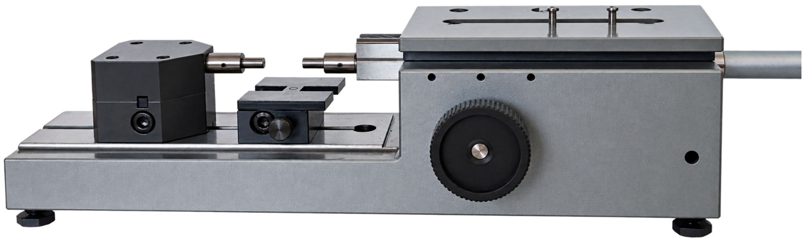
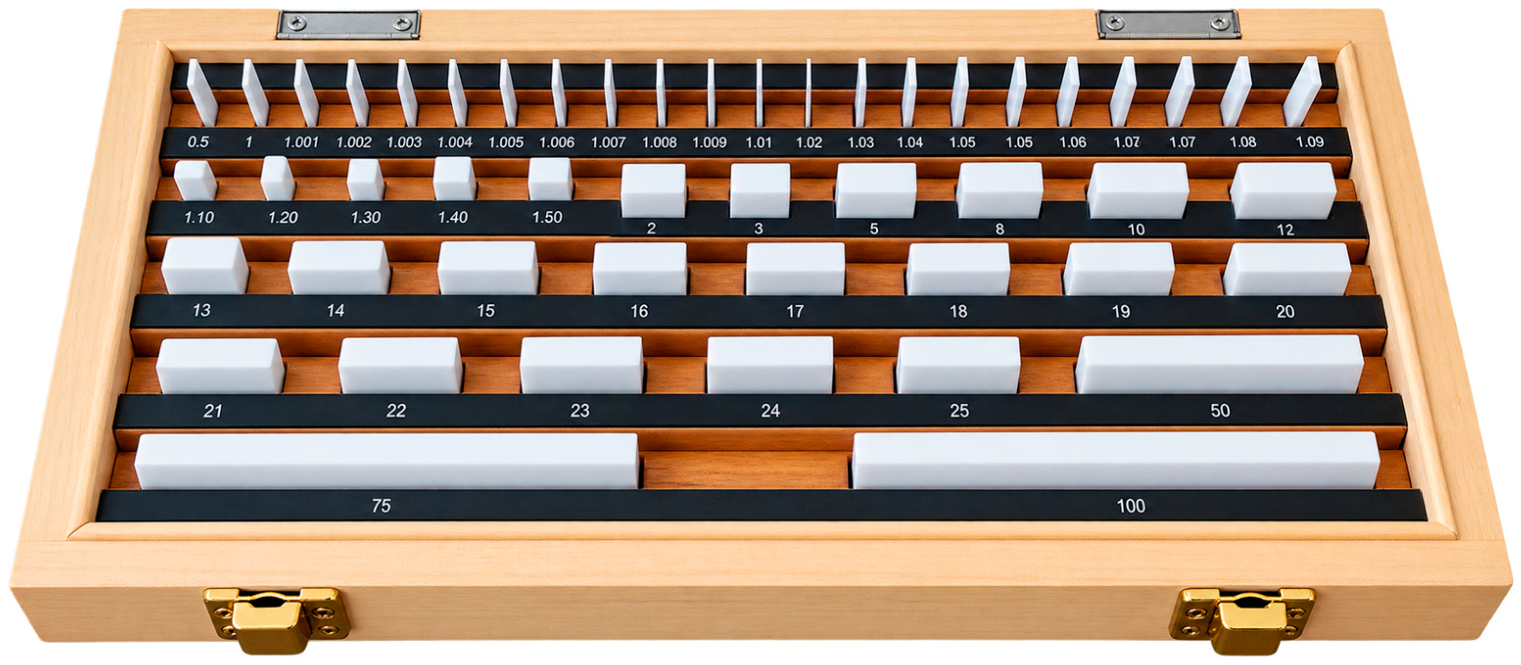
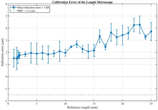
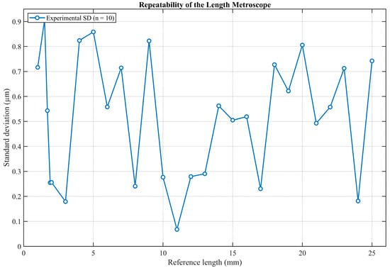
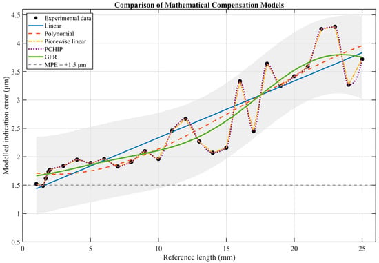
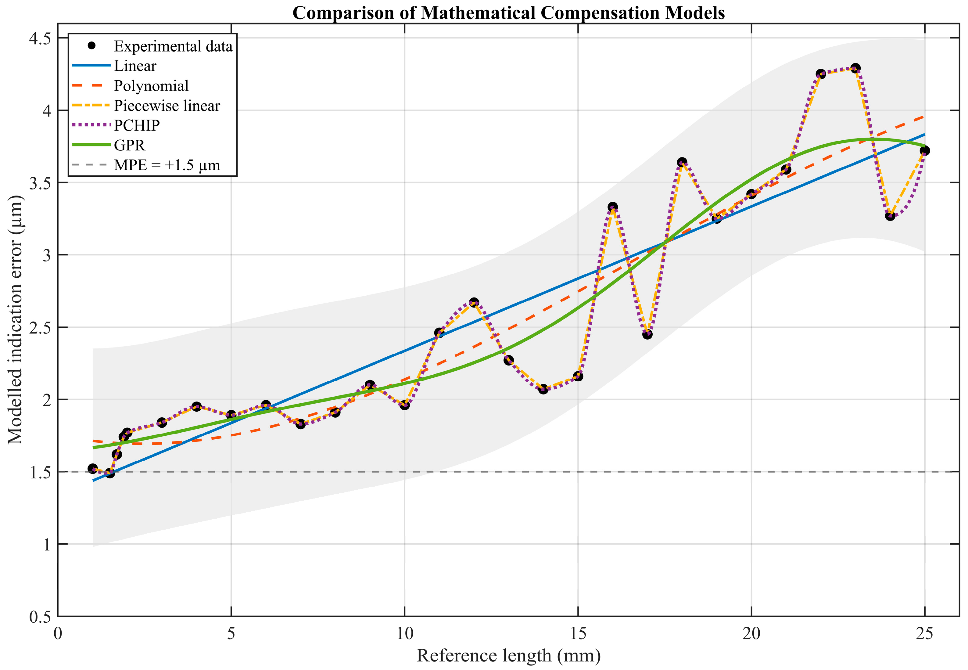
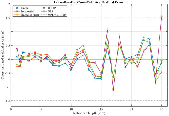
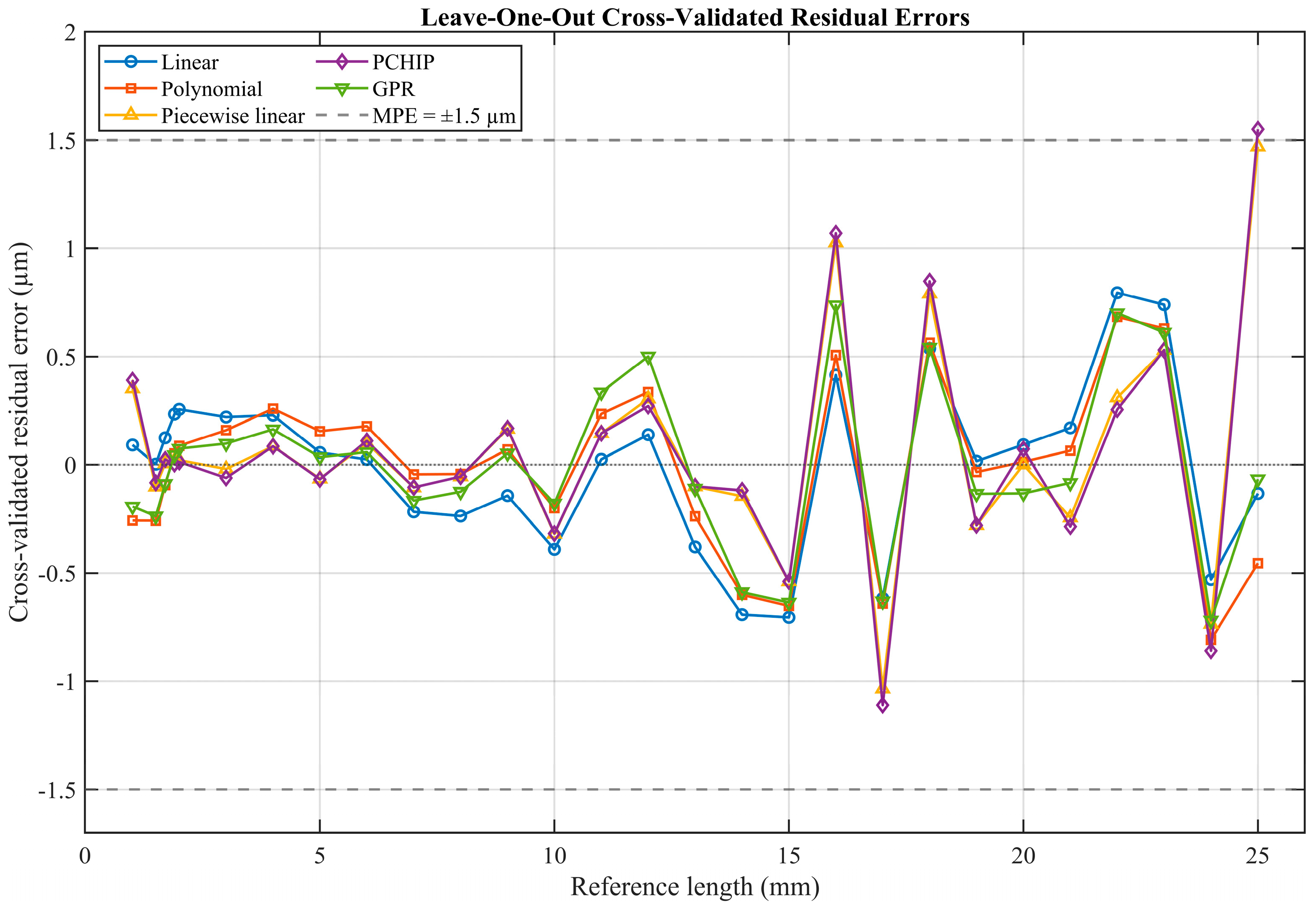
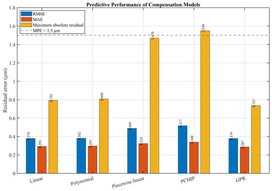
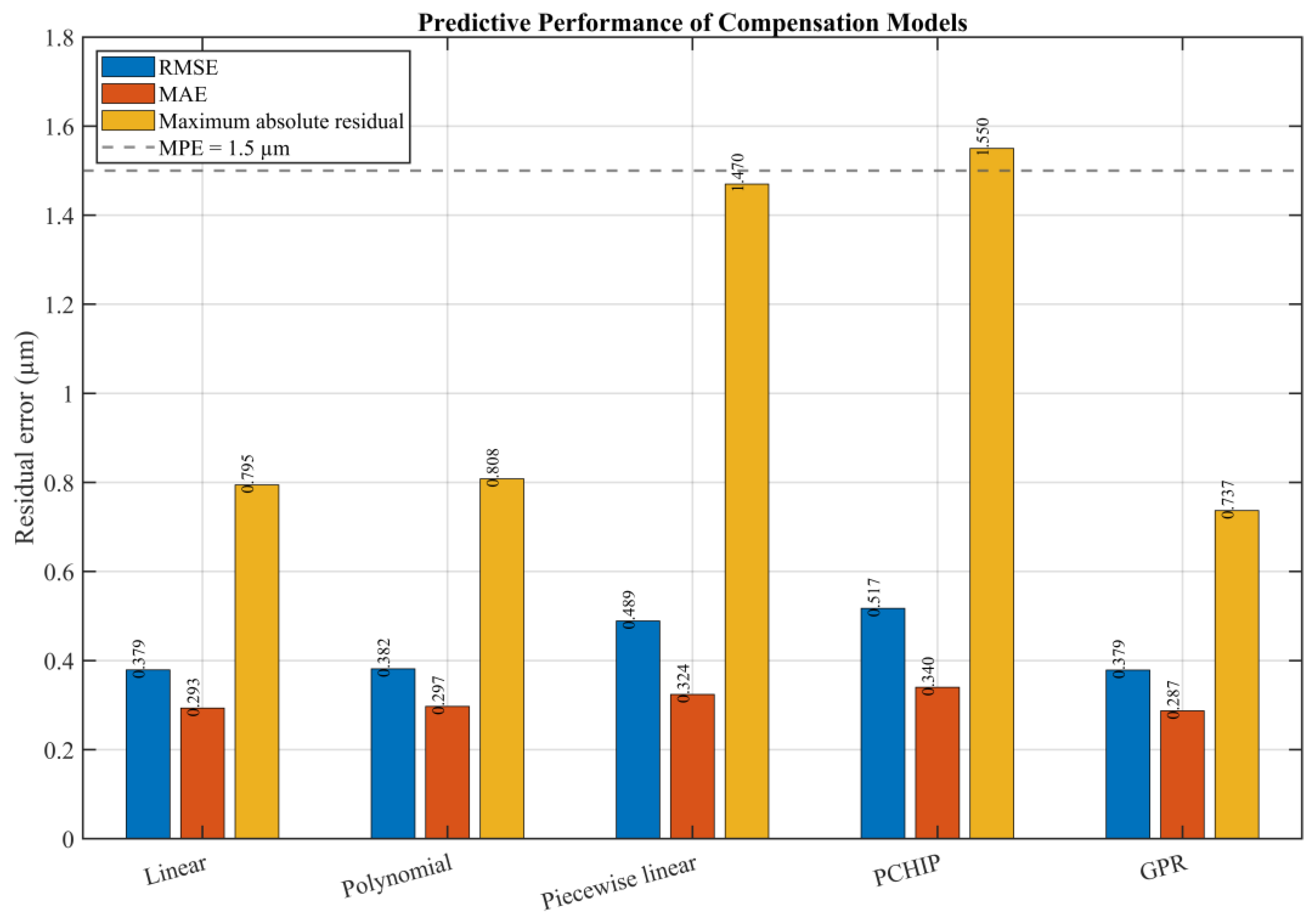
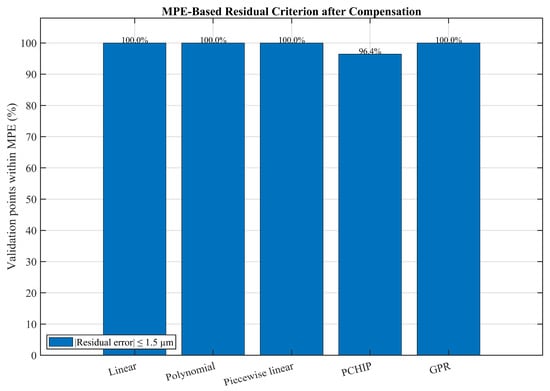
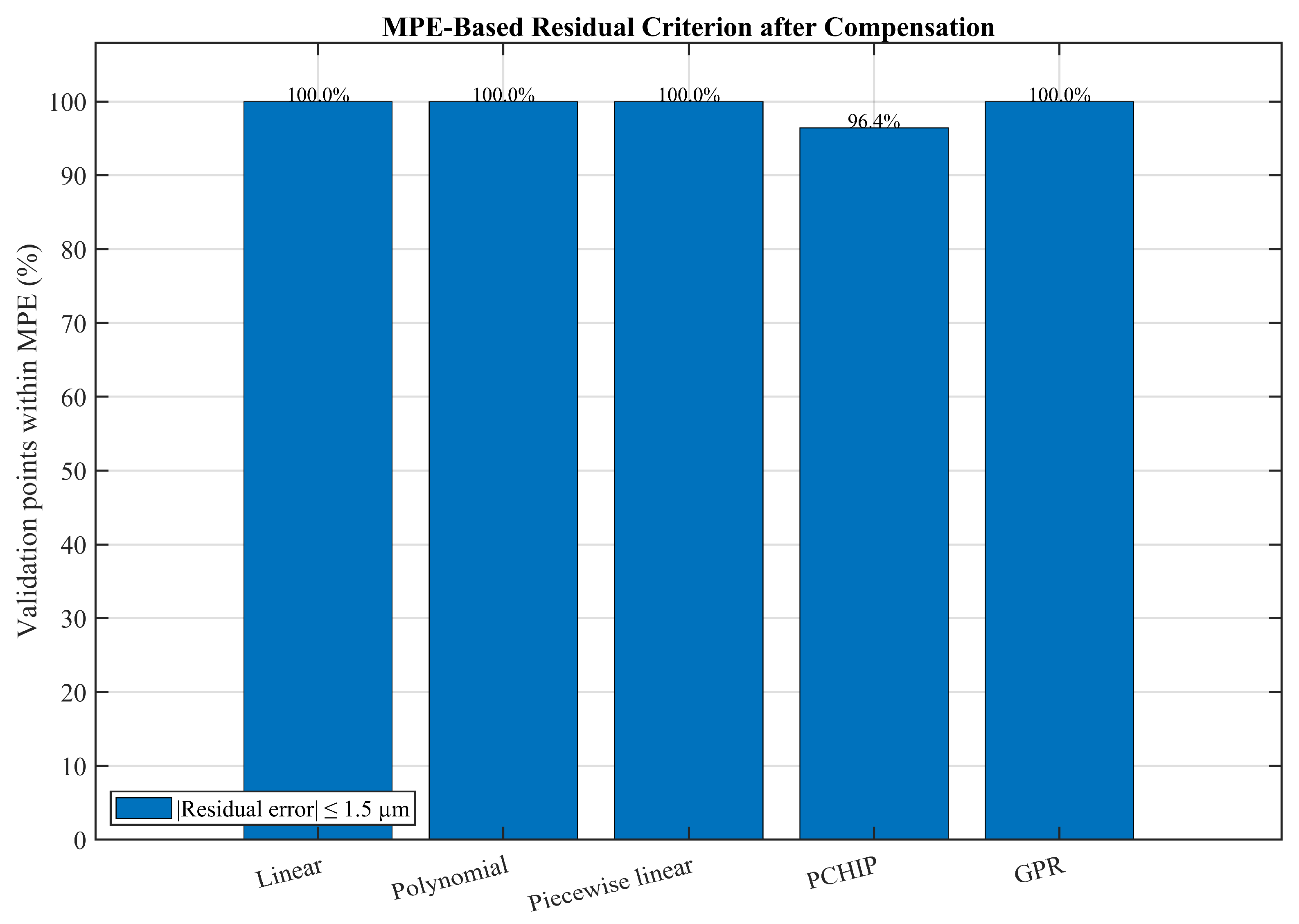

Disclaimer/Publisher’s Note: The statements, opinions and data contained in all publications are solely those of the individual author(s) and contributor(s) and not of MDPI and/or the editor(s). MDPI and/or the editor(s) disclaim responsibility for any injury to people or property resulting from any ideas, methods, instructions or products referred to in the content. |
© 2026 by the authors. Licensee MDPI, Basel, Switzerland. This article is an open access article distributed under the terms and conditions of the Creative Commons Attribution (CC BY) license.