Metrological Aspects of Soft Sensors for Estimating the DC-Link Capacitance of Frequency Inverters

Abstract

The capacitance of the DC link is an important variable for the prediction of remaining useful life and failures in frequency inverters. The direct measurement of the DC-link capacitance in inverters operating under load is technically challenging and generally impractical. Recently, a great focus has been given to data-based soft sensors for estimating this variable. These methods, however, are evaluated based only on the estimate errors, and do not take into account the metrological aspects of these estimators. This paper proposes an uncertainty analysis method based on Monte Carlo simulations and bootstrapping that can be applied to all recently published methods for end-of-life (EOL) estimation based on data-driven regression and neural networks. A state-of-the-art model of EOL monitoring based on capacitance estimation was evaluated using the proposed framework, and an experimental study with a frequency converter drive for a brushless DC motor was performed, considering multiple output frequencies, loads and DC-link capacitance conditions. The output distributions are not symmetrical and show that the variable with the most significant impact in the propagated uncertainty is the DC link voltage. The results show confidence interval widths ranging from 12 μF to 61 μF, with wider confidence intervals obtained at higher power setpoints.

1. Introduction

Power electronics systems are widely used in modern society [1]. By minimizing the losses associated with the conversion of different forms of electricity, they contribute to improving energy efficiency in multiple areas and on a global scale. They enable the integration of renewable energy sources [2,3]; support battery-energy-management systems and motor control in electric mobility [4,5]; are essential for the control and operation of electrical machines and other equipment in industrial processes [6,7]; and are part of the entire current infrastructure, ranging from switched-mode power supplies in computers and data centers to long-distance high-voltage DC transmission systems [8,9,10].

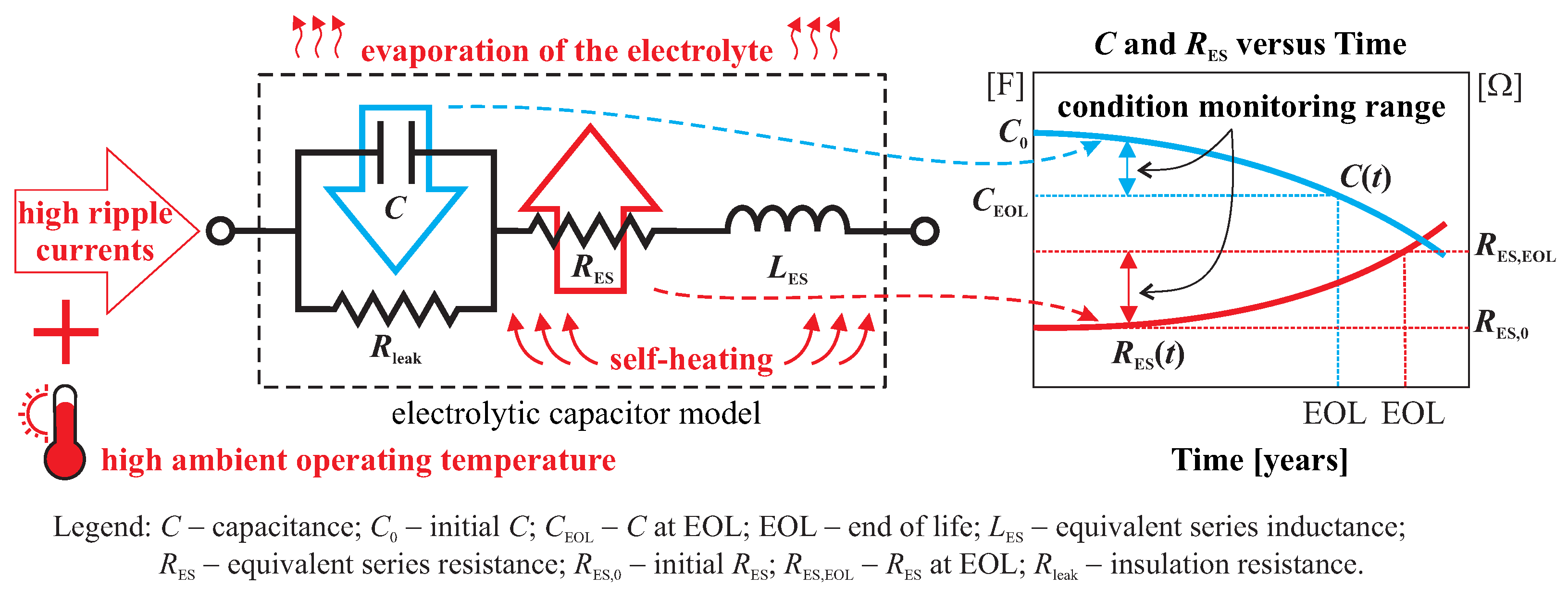
The energy conversion process includes a stage that requires a constant DC-link voltage, which is generally achieved through a set of large-capacitance aluminum electrolytic capacitors. When operating as filters in the DC link, these elements are subjected to high ripple currents, often the limiting parameter in their design, which can lead to excessive heating. Among other factors, self-heating combined with high ambient operating temperatures can cause irreversible damage to aluminum electrolytic capacitors, significantly reducing their useful life expectancy and that of equipment that makes use of them [11]. In fact, a relatively recent survey conducted with 51 companies from the European Center for Power Electronics (ECPE) indicated that capacitors are among the components most susceptible to failure in power electronics converters [12].

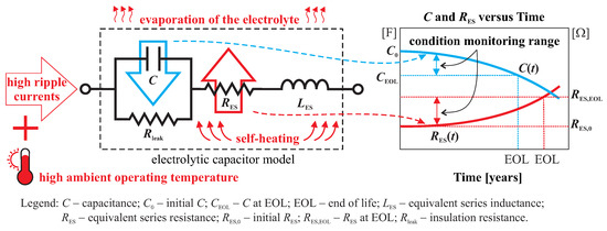
In general, electrolytic capacitors consist of an anode and a cathode made of aluminum foil, which act as electrodes; a separating paper impregnated with electrolyte between the foils; and an oxide layer on the surface of the anode foil, which acts as a dielectric. Although more or less complex representations can be found in the literature, the electrolytic capacitor model shown in Figure 1 is widely accepted. It consists of four elements: the capacitance (C) between the electrodes; the leakage resistance ($R_{\mathrm{leak}}$), also referred to as parallel resistance or insulation resistance, which represents losses in the electrolyte and dielectric and gives rise to a leakage current; the equivalent series resistance (ESR), denoted by $R_{\mathrm{ES}}$, originating from electrical connections, impregnated paper, and electrodes; and the equivalent series inductance ($L_{\mathrm{ES}}$) associated with terminals and windings [13].

Figure 1. Equivalent circuit and aging mechanisms of aluminum electrolytic capacitors and their typical condition monitoring indicators.

The aging of aluminum electrolytic capacitors occurs primarily due to the reduction of electrolyte volume, resulting from evaporation or consumption during operation [13]. The ripple currents flowing through the ESR generate power dissipation and self-heating, which accelerate electrolyte loss [11]. As the paper separator becomes less impregnated, portions of the rough surface of the anode cease to be electrically active, reducing the effective capacitance area and, consequently, the capacitance. In parallel, the dielectric undergoes chemical degradation, especially under high temperatures or overvoltage conditions, which contributes to an increase in the leakage current. Thermal and mechanical cycling can also degrade internal connections and promote foil delamination, leading to a gradual increase in the ESR [13]. For these reasons, capacitance and ESR are the most commonly used indicators of component aging: the capacitor is typically considered to have reached its end of life (EOL) when its capacitance drops to about 80% of its initial value, while the ESR increase is limited by a maximum value specified by the manufacturer. This value is typically between 100% and 200% above the initial condition, depending on the application and capacitor class [14].

Because capacitor characteristics directly affect the reliability, efficiency, and operational lifetime of power electronics systems, monitoring their condition becomes critically important, particularly in high-performance applications. Early detection of degradation in capacitance or ESR enables predictive maintenance and provides sufficient time for a controlled system shutdown. This not only prevents abrupt failures but also reduces the financial losses associated with unplanned downtime and corrective maintenance.

In a recent review, the authors in [15] introduced a classification in which methods for estimating the EOL of electrolytic capacitors are broadly categorized into four main groups. The first group is formed by fundamental-relationship-based schemes, focusing on the extraction of health indicators from electrical, thermal, or impedance measurements [16,17,18,19]. The second group comprises schemes based on capacitor charge and discharge profiles and nonperiodic signals [20,21,22]. A third group includes data-driven methods, in which statistical learning and machine learning (ML) techniques are employed to infer the variables of interest [23,24,25,26,27,28]. Other methods that do not fit into the previous categories, typically using quantities that are not directly associated with the operation of the converter, make up the fourth group [29,30].

With the increasing adoption of ML in industrial monitoring systems, data-driven approaches have become prominent in capacitor condition monitoring and EOL assessment in relation to approaches from the other groups [15]. These approaches often achieve lower average estimation errors than methods derived solely from fundamental relationships; however, their metrological characterization is less straightforward. Although the importance of assessing the metrological performance of soft sensors has been highlighted in several application domains [31,32,33,34,35,36,37], the nonlinear mappings and data-dependent behavior of ML-based soft sensors can yield non-Gaussian output distributions. This invalidates the assumptions underlying linearized uncertainty propagation, as commonly applied under the framework of the Guide to the Expression of Uncertainty in Measurement (GUM). Addressing this gap is especially critical in the context of power electronics, where recent literature has increasingly emphasized the need for rigorous uncertainty modeling and reliability evaluation [38,39]. Despite this growing awareness, to the best of the authors’ knowledge, such a metrological analysis has not yet been reported for ML-based methods targeting capacitor EOL indicators in power converters.

In the domain of uncertainty quantification, Bayesian approaches are widely recognized for their ability to capture epistemic uncertainty. For instance, Bayesian parameter estimation has recently been applied to capacitor condition monitoring to obtain the posterior distributions of empirical aging models [40]. In the context of machine learning, Bayesian Neural Networks (BNNs) extend this concept by replacing deterministic network weights and biases with probability distributions, effectively operating in the weight space [41]. However, formal Bayesian inference typically demands the definition of prior distributions, entails computationally heavy variational inference or Markov Chain Monte Carlo sampling, and often lacks explicit integration of standardized metrological components.

A method to assess the uncertainty in the estimates of performance variables in compressor tests was proposed in [42] based on a hybrid framework combining Monte Carlo simulations (MCS) and bootstrapping. This method accounts for errors arising from the incompleteness of the training set and from the optimization of data-driven models, and it enables the evaluation of the impact of input variable uncertainty propagation through these models, both during training and in their application, while being simpler to tune and still being able to act on high-dimensional data, as the models trained are standard neural networks. Those characteristics are important for the case of the DC-link capacitance estimates, but the original method cannot be directly applied to this problem, as some normality assumptions necessary for the original method do not hold in this case. In addition, some modifications should be made to consider the particularities of DC-link capacitor condition monitoring methods.

This paper proposes an uncertainty evaluation method for data-driven soft sensors used to estimate capacitor EOL indicators in frequency converters that is based on ideas from the framework established in [42]. The approach combines MCS for propagating input measurement uncertainty with bootstrapping to account for model variability due to dataset composition and stochastic training. While solid in its application, the method in [42] relies on two structural constraints that limit its direct application to this domain. First, regarding inference generation, it relies on its own specific internal ensemble to compute the final estimated value. The framework proposed in this paper improves upon this by completely decoupling the inference step from the uncertainty evaluation, acting as an external metrological wrapper. Second, the baseline method relies on standard confidence interval metrics, which implicitly assume symmetrical and well-behaved error distributions for analytical combination. Because the propagation of input uncertainty in this application inherently yields heavily skewed output probability density function, the proposed method introduces an adaptive distribution processing strategy. By utilizing numerical percentiles when a distribution is determined to be non-Gaussian, this approach overcomes the limitations of traditional, symmetry-assuming confidence intervals to mathematically guarantee reliable metrological bounds.

The proposed method is validated in a case study using the structure of state-of-the-art neural-network capacitance estimators reported in [28], which were implemented and tested in an experimental inverter-drive setup with controlled variations of DC-link capacitance. While the case study focuses on capacitance estimation, the proposed framework can be applied to other ML-based estimators and can also be applied to determine the uncertainty of other capacitor health indicators, such as the ESR.

The remainder of this paper is organized as follows. Section 2 presents the proposed framework for evaluating the uncertainty associated with data-based soft-sensor estimation. Section 3 describes the experimental study, evaluating the applicability of the proposed solution to a case of DC-link capacitance estimation. Section 4 discusses the results obtained in the case study. Finally, Section 5 presents the conclusions of this paper.

2. Proposed Uncertainty Evaluation Framework

This section describes the framework developed for the metrological characterization of data-driven soft sensors for evaluating capacitor health in the DC link of power converters. The method is designed to estimate the uncertainty associated with a capacitor health indicator (capacitance or ESR) by accounting for both measurement-related and model-induced uncertainties. Specifically, the developed architecture consists of an ensemble of neural networks that are trained considering the probability density functions of the input quantities, defined based on their measurement uncertainties. The combination of the aforementioned sources of uncertainty and the uncertainty of the target variable is addressed in a second step, which is also detailed in this section.

2.1. Uncertainty Ensemble

An ensemble of neural networks, $E_{\mathrm{unc}}$, composed of $N_{\mathrm{unc}}$ neural networks, is designed to capture the epistemic and aleatoric uncertainties of the capacitor health estimates. This ensemble explicitly accounts for the metrological characteristics of the sensors and the stochastic nature of the inputs. The creation of the ensemble can be divided into two phases, detailed below.

2.1.1. Probabilistic Input Modeling

Let ${\mathcal{D}}_{\mathrm{base}}={\left\{({\mathbf{x}}_j,y_j)\right\}}_{j=1}^{N_{\mathrm{samples}}}$ be the available measurements for training the capacitor health predictor, where ${\mathbf{x}}_j\in {\mathbb{R}}^d$ represents the input feature vector of the j-th sample available, d is the number of input features considered, $N_{\mathrm{samples}}$ represents the total number of samples in the dataset, and $y_j$ corresponds to the target label (ground truth) associated with the j-th sample available. For each j-th instance of ${\mathcal{D}}_{\mathrm{base}}$, the input vector is defined as ${\mathbf{x}}_j={[x_{1,j,\mathrm{meas}},x_{2,j,\mathrm{meas}},\dots ,x_{d,j,\mathrm{meas}}]}^{\top }$, where each component of the vector represents a raw physical quantity obtained directly from the power converter without any uncertainty information. These values are used for training the conventional inference model that predicts the capacitor health indicator.

In a real-world scenario, the measured value of the i-th component of vector ${\mathbf{x}}_j$, denoted as $x_{i,j,\mathrm{meas}}$, differs from the true value $x_{i,j,\mathrm{true}}$ by an unknown error ${\delta }_{i,j}$. This probabilistic treatment of unknown measurement errors follows the accepted framework for uncertainty propagation, specifically the Monte Carlo method outlined in Supplement 1 to the Guide to the Expression of Uncertainty in Measurement [43]. Because the exact error distribution within the instrument accuracy limits is unknown, a rectangular (uniform) PDF is assigned, with values according to the datasheet of the instrument used for measurement.

To create a dataset ${\mathcal{D}}_{\mathrm{MCS}}$ for training the uncertainty ensemble, a set is generated by sampling from the input PDFs. This dataset maintains the same size as the baseline data but injects variability into the inputs. It is defined as:

$${\mathcal{D}}_{\mathrm{MCS}}=\left\{({\tilde{\mathbf{x}}}_j,y_j)\mid ({\mathbf{x}}_j,y_j)\in {\mathcal{D}}_{\mathrm{base}},j=1,\dots ,N_{\mathrm{samples}}\right\},$$

(1)

where ${\tilde{\mathbf{x}}}_j$ is the modified input vector. It is important to note that the ground truth target $y_j$ remains invariant, but the input vector is modified by sampling a new value from the respective PDF according to the instrument and measurement specifications. Uncertainty in $y_j$ is considered in the final stage of the proposed method. The modified input vector ${\tilde{\mathbf{x}}}_j$ is defined as:

$${\tilde{\mathbf{x}}}_j={\mathbf{x}}_j+{\gamma }_j=\left[\begin{array}{c}{x}_{1,j,\mathrm{meas}}+{\gamma }_{1,j}\\ x_{2,j,\mathrm{meas}}+{\gamma }_{2,j}\\ ⋮\\ x_{d,j,\mathrm{meas}}+{\gamma }_{d,j}\end{array}\right],$$

(2)

where ${\gamma }_{i,j}$ is a sample drawn from the PDF ${\mathcal{P}}_i$ associated with that feature, based on uncertainty information, such as accuracy coefficients and distribution types, from the datasheet of the instrument (${\Theta }_{\mathrm{unc},\mathrm{train}}$).

2.1.2. Bootstrapping and Out-of-Bag Validation

To quantify epistemic uncertainty, a bootstrapping with replacement technique is applied to ${\mathcal{D}}_{\mathrm{MCS}}$. For a dataset of size N, a new training set is formed by sampling N times from the original dataset with replacement, creating a bootstrapped dataset (${\mathcal{D}}_{\mathrm{boot}}$). The unselected samples form the out-of-bag (OOB) dataset (${\mathcal{D}}_{\mathrm{OOB}}$). In this framework, the OOB set replaces the standard validation set used in the training process of the original inference model, serving as an unbiased estimator for the stopping criterion and ensuring model diversity.

An acceptance criterion for uncertainty models is used, with a maximum error threshold (${\Gamma }_{\mathrm{unc}}$) to accommodate sampling from the input PDF. The maximum error used for comparison against ${\Gamma }_{\mathrm{unc}}$ is determined by evaluating every instance from the out-of-bag validation set using the same loss function applied during training. If the highest single prediction error across this validation set exceeds ${\Gamma }_{\mathrm{unc}}$, the model is deemed to have failed and is discarded. The numerical threshold was empirically established at ${\Gamma }_{\mathrm{unc}}=175 \mathsf{\mu }\mathrm{F}$. This specific value was chosen to balance computational processing time against ensemble quality. By filtering out poorly converged networks, this threshold prevents catastrophic outliers from artificially inflating the spread of the output distribution, thereby ensuring that the resulting uncertainty estimates remain realistic.

2.2. Algorithm and Final Estimation

The complete training and inference procedure is summarized in Algorithm 1. The final estimation combines the prediction from the inference model, $M_{\inf }$, with the dispersion analysis from $E_{\mathrm{unc}}$.

Algorithm 1 Training and Estimation of the Virtual Sensor with Uncertainty
Require:  Training dataset ${\mathcal{D}}_{\mathrm{base}}$, number of models in ensemble $N_{\mathrm{unc}}$, training instrument uncertainty ${\Theta }_{\mathrm{unc},\mathrm{train}}$, ensemble threshold ${\Gamma }_{\mathrm{unc}}$, application dataset ${\mathcal{D}}_{\mathrm{app}}$, application instrument uncertainty ${\Theta }_{\mathrm{unc},\mathrm{app}}$, target coverage probability p, target uncertainty $U_{\mathrm{ref}}$, normality threshold $\beta$, number of simulation trials K
Ensure:  Final prediction $\widehat{y}$, confidence interval width $W_p$
1: Phase 1: inference model training ($M_{\inf }$)
2: Train $M_{\inf }$ on ${\mathcal{D}}_{\mathrm{base}}$
3: Phase 2: uncertainty ensemble training ($E_{\mathrm{unc}}$)
4: for $j\leftarrow 1$ to $N_{\mathrm{unc}}$   do
5:     repeat
6:    Generate training uncertainty set ${\gamma }_j\sim \mathcal{P}\left({\Theta }_{\mathrm{unc},\mathrm{train}}\right)$
7:    Define ${\mathcal{D}}_{\mathrm{MCS}}$ through (2) for every element in ${\mathcal{D}}_{\mathrm{base}}$ and ${\gamma }_j$	▹ Sample uncertainty PDF (training stage)
8:    ${\mathcal{D}}_{\mathrm{boot}}\leftarrow$ Resample(${\mathcal{D}}_{\mathrm{MCS}}$)	▹ Bootstrap with replacement
9:    ${\mathcal{D}}_{\mathrm{OOB}}\leftarrow {\mathcal{D}}_{\mathrm{MCS}}\setminus {\mathcal{D}}_{\mathrm{boot}}$	▹ Out-of-bag samples
10:    Train model $M_j$ on ${\mathcal{D}}_{\mathrm{boot}}$
11:    Calculate $MaxError$ on ${\mathcal{D}}_{\mathrm{OOB}}$
12:     until $MaxError\le {\Gamma }_{\mathrm{unc}}$
13:     Add $M_j$ to $E_{\mathrm{unc}}$
14: end for
15: Phase 3: final estimation (application phase)
16: $\alpha \leftarrow 1-p$	▹ Significance level
17: Generate application uncertainty set ${\gamma }_{j,\mathrm{app}}\sim \mathcal{P}\left({\Theta }_{\mathrm{unc},\mathrm{app}}\right)$
18: Estimate $\widehat{y}$ from ${\mathcal{D}}_{\mathrm{app}}$ using $M_{\inf }$
19: Generate K variations of ${\mathcal{D}}_{\mathrm{MCS},\mathrm{app}}$ through (2) for every element in ${\mathcal{D}}_{\mathrm{app}}$ and ${\gamma }_{j,\mathrm{app}}$	▹ Sample uncertainty PDF (application stage)
20: ${\mathbf{Y}}_{\mathrm{unc}}\leftarrow$ Predict ${\mathcal{D}}_{\mathrm{MCS},\mathrm{app}}$ using $E_{\mathrm{unc}}$	▹ Ensemble output distribution
21: Uncertainty combination strategy
22: $p_{\mathrm{val}}\leftarrow \mathrm{NormalityTest}\left({\mathbf{Y}}_{\mathrm{unc}}\right)$	▹ e.g., Anderson-Darling
23: $u_{\mathrm{ref}}\leftarrow U_{\mathrm{ref}}/k$	▹ Instrument standard uncertainty
24: if $p_{\mathrm{val}}>\beta$ then	▹ Distribution is Gaussian
25:     $u_{\mathrm{model}}\leftarrow \mathrm{StdDev}\left({\mathbf{Y}}_{\mathrm{unc}}\right)$
26:     Calculate $u_{\mathrm{c}}$ using (3)	▹ Analytical GUM method
27:     $W_p\leftarrow 2·k·u_{\mathrm{c}}$	▹ Full Gaussian width
28: else	▹ Distribution is non-Gaussian
29:     Generate uncertainty vector ${\gamma }_{\mathrm{ref}}\sim \mathcal{P}(0,u_{\mathrm{ref}})$
30:     ${\mathbf{Y}}_{\mathrm{combined}}\leftarrow {\mathbf{Y}}_{\mathrm{unc}}+{\gamma }_{\mathrm{ref}}$	▹ Numerical sum
31:     $P_{\mathrm{upper}}\leftarrow \mathrm{Quantile}({\mathbf{Y}}_{\mathrm{combined}},1-\alpha /2)$	▹ Ex: $\alpha =0.05$ for $p=0.95$
32:     $P_{\mathrm{lower}}\leftarrow \mathrm{Quantile}({\mathbf{Y}}_{\mathrm{combined}},\alpha /2)$
33:     $W_p\leftarrow P_{\mathrm{upper}}-P_{\mathrm{lower}}$	▹ Full non-Gaussian width
34: end if
35: return $\widehat{y},W_p$

Initially, phase 1 of Algorithm 1 provides an estimator $M_{\inf }$, which is essentially the application of the original method to estimate the capacitor health parameter of interest. For this purpose, a single neural network is trained solely on the training data (${\mathcal{D}}_{\mathrm{base}}$) using the features, methods, and hyperparameters described in data-driven methods from the literature, designed to provide an estimate $\widehat{y}$ of the target variable.

Phase 2 constructs the uncertainty ensemble ($E_{\mathrm{unc}}$), consisting of $N_{\mathrm{unc}}$ independent neural networks, responsible for quantifying the confidence interval of the prediction. To capture the most faithful PDF from the original instruments, MCS and bootstrapping are used. MCS is conducted to generate a dataset with aleatoric uncertainty arising from the measurement instruments (${\mathcal{D}}_{\mathrm{MCS}}$). Secondly, aiming for model diversity and to capture epistemic uncertainty, bootstrapping resamples ${\mathcal{D}}_{\mathrm{MCS}}$ uniformly with replacement, creating a new dataset (${\mathcal{D}}_{\mathrm{boot}}$). This process leaves out a subset of samples unselected, which will become the out-of-bag dataset (${\mathcal{D}}_{\mathrm{OOB}}$). Each model is trained on ${\mathcal{D}}_{\mathrm{boot}}$ and validated on ${\mathcal{D}}_{\mathrm{OOB}}$. This process is done once for each attempt a model makes to enter the ensemble, until $N_{\mathrm{unc}}$ models are approved.

Once the ensemble is trained, phase 3 begins with a process similar to phase 2 of performing MCS, but it is applied to any unseen dataset used for application (${\mathcal{D}}_{\mathrm{app}}$), including the test dataset (${\mathcal{D}}_{\mathrm{test}}$). The difference here is that different variations of an MCS dataset (${\mathcal{D}}_{\mathrm{MCS},\mathrm{app}}$) are performed $N_{\mathrm{trial}}$ times, so that every model in $E_{\mathrm{unc}}$ can estimate the target variable in all trials of all application samples. This resulting distribution (${\mathbf{Y}}_{\mathrm{unc}}$), which contains $N_{\mathrm{unc}}·N_{\mathrm{trials}}$ points, captures both aleatoric uncertainty from the inputs and epistemic uncertainty from model disagreement within the ensemble. It is important to note that the application data are not necessarily acquired from the same instrument as the training data. Consequently, the training instrument uncertainty used for Monte Carlo propagation (${\Theta }_{\mathrm{unc},\mathrm{train}}$) can differ from that used for application (${\Theta }_{\mathrm{unc},\mathrm{app}}$). This distinction allows for the assessment of model performance under other sensor conditions, such as the test dataset or other application settings. An uncertainty set ${\gamma }_{j,\mathrm{app}}$ is generated with the same structure as ${\gamma }_j$, but with information from ${\Theta }_{\mathrm{unc},\mathrm{app}}$.

To ensure robust uncertainty quantification that respects the non-Gaussian nature of the output distributions typically found in this type of application, a direct probabilistic combination strategy is employed in the application phase. Following [44], if the resulting model distribution is characterized as Gaussian, the combined uncertainty $u_{\mathrm{c}}$ is typically obtained through the propagation of uncertainty. For uncorrelated quantities, this is expressed as:

$$u_{\mathrm{c}}=\sqrt{u_{\mathrm{model}}^2+u_{\mathrm{ref}}^2},$$

(3)

where $u_{\mathrm{model}}$ represents the standard uncertainty of the predictive model and $u_{\mathrm{ref}}$ is the standard uncertainty of the reference quantity instrumentation. The expanded uncertainty $U_p$ for a given confidence level p is then calculated as:

$$U_p=k·u_{\mathrm{c}},$$

(4)

where k is the coverage factor calculated from a t-distribution and the corresponding degrees of freedom ($k=2$ for a 95.45% coverage probability with infinite degrees of freedom) [44].

However, this approach relies on the assumption that the output PDF, generated from the outputs of the uncertainty ensemble, is symmetric and Gaussian. The data-driven model output may exhibit non-Gaussian characteristics, such as skewness or multimodality. In such cases, these assumptions could lead to a loss of statistical information. Furthermore, combining a nonparametric distribution from the ensembles with a parametric distribution from the instruments could yield an inaccurate estimate of the coverage intervals.

To address these limitations, the proposed method employs a strategy based on the numerical propagation of distributions. Instead of combining variances as in (3), the method performs the direct probabilistic superposition of the uncertainty from the instrument onto the empirical distribution of the model. Mathematically, the proposed framework allows for the selection of an uncertainty propagation method based on the properties of the output distribution of the uncertainty ensemble.

First, the ensemble prediction vector (${\mathbf{Y}}_{\mathrm{unc}}$) is subjected to an Anderson–Darling normality test [45]. If the distribution fails to reject the null hypothesis of normality—indicated by a calculated test statistic lower than the critical value associated with the significance threshold $\beta$—the distribution is treated as Gaussian, and the method defaults to the standard analytical combination presented in (3) [45]. In this case, the combined standard model uncertainty $u_{\mathrm{model}}$ is simply the standard deviation of ${\mathbf{Y}}_{\mathrm{unc}}$, and the final expanded uncertainty is calculated as in (4) with $u_{\mathrm{c}}$ obtained using (3). For this framework, the threshold was set to a standard 5% significance level ($\beta =0.05$), corresponding to a critical test statistic of 0.787. This specific value was chosen because it provides statistical balance, being strict enough to reliably detect the skewed, heavy-tailed distributions inherent to this application (safely triggering the nonparametric propagation), while avoiding false rejections of normality caused by minor variations in the Monte Carlo sampling. To allow a comparison with the nonparametric interval width, the width of the equivalent confidence interval for the Gaussian case, $W_p$, is computed as:

$$W_p=2·U_p.$$

(5)

Alternatively, if nonnormality is detected, the numerical propagation strategy is used. In this scenario, the uncertainty of the reference instrument is generated as a stochastic vector ${\gamma }_{\mathrm{ref}}\sim \mathcal{P}(0,u_{\mathrm{ref}})$ and added element-wise to the ensemble prediction vector (${\mathbf{Y}}_{\mathrm{unc}}$) as:

$${\mathbf{Y}}_{\mathrm{combined}}={\mathbf{Y}}_{\mathrm{unc}}+{\gamma }_{\mathrm{ref}}.$$

(6)

This operation effectively superimposes the measurement uncertainty onto the model empirical distribution. The final p confidence interval width ($W_p$) is then computed nonparametrically as the width between the lower quantile ($q_{\alpha /2}$) and the upper quantile ($q_{1-\alpha /2}$), where $\alpha =1-p$ represents the significance level. These steps ensure that the resulting interval satisfies the target confidence level p regardless of the distribution shape.

Regarding the hyperparameters of the framework, the ensemble size ($N_{\mathrm{unc}}$) must be chosen to balance computational cost and statistical stability. The uncertainty ensemble typically requires a large population to accurately reconstruct the probability density function, ensuring a high-resolution estimation of the coverage interval.

While both BNNs and the proposed MCS-bootstrap ensemble aim to generate predictive distributions to capture uncertainty, their fundamental mechanics diverge significantly. BNNs employ a probabilistic approach strictly within the parameter or weight space of the network. In contrast, the proposed framework operates within the data and model spaces. By relying on Monte Carlo simulations, it explicitly incorporates standardized metrological components, i.e., the Monte Carlo method [43], directly into the data space. Simultaneously, bootstrapping explores the model space to capture epistemic uncertainty. This strategy constructs an empirical, nonparametric predictive distribution that bypasses formal Bayesian inference, resulting in a framework that is highly parallelizable, avoids typical optimization instabilities, and is conceptually simpler for industrial metrology applications.

3. Experimental Case Study

To demonstrate the practical applicability and validate the proposed uncertainty framework, a comprehensive case study was conducted focusing on the estimation of DC-link capacitance in a frequency converter. This section details the experimental infrastructure used to generate the degradation dataset, the signal processing techniques employed for feature extraction, and the specific artificial neural network (ANN) topologies selected for evaluation.

3.1. Test Rig Modeling and Uncertainties

To validate the proposed method for uncertainty evaluation of the estimation models, an experimental test bed was developed to emulate the degradation of the capacitors in the DC link. The system aims to achieve this under variable operating conditions of a frequency converter driving a brushless DC (BLDC) motor in different load and capacitance scenarios.

The electromechanical system consists of a three-phase BLDC motor with two pole pairs and an inner rotor configuration. The mechanical load is imposed by a AHB-1 hysteresis brake (Magtrol, West Seneca, USA), which provides torque control independent of angular velocity. The brake is driven by a programmable DC power supply (GEN600-1.3, TDK-Lambda, Wuxi, China), allowing for load regulation during tests.

A CF10B01 frequency converter (Nidec Global Appliances, Joinville, Brazil) drives the motor according to the specifications presented in Table 1, with the output voltage varying according to the motor load. A custom-developed capacitor jig inserted into the DC link of the converter allows for the controlled variation of the DC-link capacitance. It comprises multiple capacitor arms (combinations of 100 $\mathsf{\mu }$$\mathrm{F}$ and 220 $\mathsf{\mu }$$\mathrm{F}$ capacitors) that are individually switched via metal–oxide–semiconductor field effect transistors (MOSFETs) controlled by a USB-6341 Data Acquisition board (National Instruments, Debrecen, Hungary). This configuration enables the DC-link capacitance to be adjusted from 70% to 100% of the nominal value, emulating capacitor degradation.

Table 1. Specifications of the frequency converter drive setup.

Parameter	Value
Input voltage (alternating current)	220 V
Input frequency	60 Hz
Nominal DC-link voltage	311 V
Nominal DC-link capacitance	1000 $\mathsf{\mu }$$\mathrm{F}$
Output frequency	40 Hz to 60 Hz

Data acquisition and instrument control are performed using a self-designed program developed in the LabVIEW programming language. Electrical quantities, including DC-link voltage, motor line currents, and voltages, are acquired using a PZ4000 power analyzer (Yokogawa, Tokyo, Japan), which has a bandwidth of 2 $\mathrm{M}$$\mathrm{Hz}$, a maximum sampling rate of 5 $\mathrm{M}$S/s, and a buffer with capacity for 100,000 samples. In order to obtain 1 $\mathrm{s}$ of continuous measurements and still be able to characterize the effects of the switching and harmonics of high frequency, a sampling rate of 100 $\mathrm{k}$$\mathrm{Hz}$ was chosen. The measurement uncertainties considered for the input variables (selected from the same feature set as in [28]) are all based on the specifications of the instrument, as detailed in Table 2, which denotes the instrument accuracy up to the frequencies used in the case study.

Table 2. Measurement uncertainty for voltage and current with the PZ4000 Power Analyzer [46].

Frequency	Accuracy
DC	$\pm (0.2\%·V_{\mathrm{M}}+0.1\%·F_{\mathrm{S}})$
$0.1$$$ ≤ $f_{\mathrm{o}}$ < 10 $\mathrm{Hz}$	$\pm (0.2\%·V_{\mathrm{M}}+0.05\%·F_{\mathrm{S}})$
10 $\mathrm{Hz}$ ≤ $f_{\mathrm{o}}$ < 60 $\mathrm{Hz}$	$\pm (0.2\%·V_{\mathrm{M}}+0.025\%·F_{\mathrm{S}})$
60 $\mathrm{Hz}$ ≤ $f_{\mathrm{o}}$ ≤ 1 $\mathrm{k}$$\mathrm{Hz}$	$\pm (0.1\%·V_{\mathrm{M}}+0.025\%·F_{\mathrm{S}})$

Note: $f_{\mathrm{o}}$ denotes the frequency of the signal being measured, $V_{\mathrm{M}}$ denotes the measured value (reading), and $F_{\mathrm{S}}$ denotes the full scale (range).

The full dataset acquired is composed of 500 samples, encompassing a capacitance range spanning from 689 $\mathsf{\mu }$$\mathrm{F}$ to 1000 $\mathsf{\mu }$$\mathrm{F}$. Specifically, the available data corresponds to ten capacitance values: {689, 734, 777, 817, 854, 889, 919, 947, 974, 1000} $\mathsf{\mu }$$\mathrm{F}$. Rather than performing a random split, a capacitance-level-based partition was adopted to separate test data from training data. The samples corresponding to 777 $\mathsf{\mu }$$\mathrm{F}$ and 919 $\mathsf{\mu }$$\mathrm{F}$ were chosen to form the test set, comprising 20% of the total dataset. The remaining eight values constituted the training and validation sets.

Considering the specifications of the Yokogawa PZ4000, the uncertainty is modeled as a rectangular distribution. The limits of this uncertainty, $\pm {\Delta }_{\lim }$, are dynamic, depending on both the reading value ($v_{\mathrm{reading}}$) and the measurement range ($v_{\mathrm{range}}$), as defined in (7):

$${\Delta }_{\lim }=(k_1·|v_{\mathrm{reading}}\left|\right)+\left(k_2·v_{\mathrm{range}}\right),$$

(7)

where $k_1$ and $k_2$ represent coefficients provided by the manufacturer (e.g., $0.1\%$ of reading and $0.025\%$ of range). Consequently, a dataset ${\mathcal{D}}_{\mathrm{MCS}}$ is generated by injecting a sample from the uncertainty distribution $\gamma \sim \mathcal{U}(-{\Delta }_{\lim },+{\Delta }_{\lim })$ into the original dataset ${\mathcal{D}}_{\mathrm{base}}$ at each iteration of the MCS process.

Regarding the reference target variable (capacitance), a standard uncertainty of $u_{\mathrm{ref}}=0.1\%$ was defined based on the experimental repeatability and the uncertainty of the instrument used to characterize the capacitors. In accordance with Algorithm 1 proposed in Section 2, this value is added as a normal distribution to the uncertainty distribution of the models, and only after this sum is the width between the 2.5th and 97.5th percentiles acquired.

3.2. Data Preprocessing and Feature Extraction

The raw data acquired from the test rig consist of high-dimensional time-series signals for the DC-link voltage, $v_{\mathrm{DC}}\left(t\right)$, and the motor phase current, $i_{\mathrm{ph}}\left(t\right)$. To facilitate the training of neural networks and enhance the model sensitivity to capacitance degradation, a feature extraction stage was implemented to condense the temporal information based on inputs from [28] into physically meaningful scalar indicators.

Five input features were derived for each sample window. In the time domain, the root mean square (RMS) of the motor current ($I_{\mathrm{RMS}}$) was calculated to characterize the load operating point. Simultaneously, the peak-to-peak amplitude of the DC-link voltage ($V_{\mathrm{DC}}^{\mathrm{pp}}$) was extracted, as the magnitude of the voltage ripple is inversely proportional to the DC-link capacitance.

In the frequency domain, a spectral analysis of the DC-link voltage was performed to isolate the dynamic behavior of the capacitor bank. The DC component was first removed from the signal, followed by the computation of the power spectral density (PSD). Three specific spectral components ($P_{{\mathrm{h}}_x}$) were selected as features: the magnitudes at the fundamental frequency (index ${\mathrm{h}}_1$), the second harmonic (${\mathrm{h}}_2$), and the fifth harmonic (${\mathrm{h}}_5$) relative to the inverter operating frequency setpoint ($f_{\mathrm{s}}$).

Finally, to ensure numerical stability and faster convergence during the training of the neural network, all five features ($I_{\mathrm{RMS}}$, $V_{\mathrm{DC}}^{\mathrm{pp}}$, $P_{{\mathrm{h}}_1}$, $P_{{\mathrm{h}}_2}$, $P_{{\mathrm{h}}_5}$) were standardized using Z-score normalization (standard scaler), resulting in a distribution with zero mean and unit standard deviation for the input vector.

Regarding the dataset partitioning, the final baseline dataset ${\mathcal{D}}_{\mathrm{base}}$ contains a total of $N=400$ samples, covering the entire experimental range. Consequently, during the training of the uncertainty ensemble ($E_{\mathrm{unc}}$), the OOB validation set, statistically estimated at $36.8\%$ of the population, consists of approximately 147 samples per estimator.

3.3. Evaluated Model Architectures

To validate the proposed metrological framework on established, state-of-the-art estimators, three MLP architectures were adopted directly from [28] to serve as case studies. These models, presented in the original study among different regression models, are named medium, wide, and trilayered, according to their architecture and hyperparameters, as defined in Table 3.

Table 3. Hyperparameters and topology specifications of the MLP models.

Parameter	Medium MLP	Wide MLP	Trilayered MLP
Hidden layers	1	1	3
Neurons per hidden layer	[25]	[100]	[10, 10, 10]
Total parameters	176	701	291
Activation (hidden)	ReLU	ReLU	ReLU
Activation (output)	Linear	Linear	Linear
Optimizer	Adam	Adam	Adam
Learning rate	$2·{10}^{-3}$	$2·{10}^{-3}$	$2·{10}^{-3}$

All models use a fixed input vector of dimension 5 ($d=5$), corresponding to the selected scalar features (${\mathbf{x}}_j\in {\mathbb{R}}^5$), and a single linear output neuron representing the estimated capacitance. The rectified linear unit (ReLU) was selected as the activation function for all hidden layers to mitigate the vanishing gradient problem. The training process is driven by the Adam optimizer. While the core architecture mirrors the reference study, standard default values were adopted for hyperparameters that could not be explicitly extracted from the toolbox used in [28]. The specific hyperparameters considered in this study are summarized in Table 3.

4. Results

After using the method proposed in Section 2 with the dataset and ANN models presented in Section 3, this section provides the results and discussion.

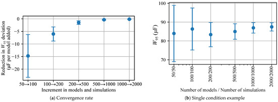
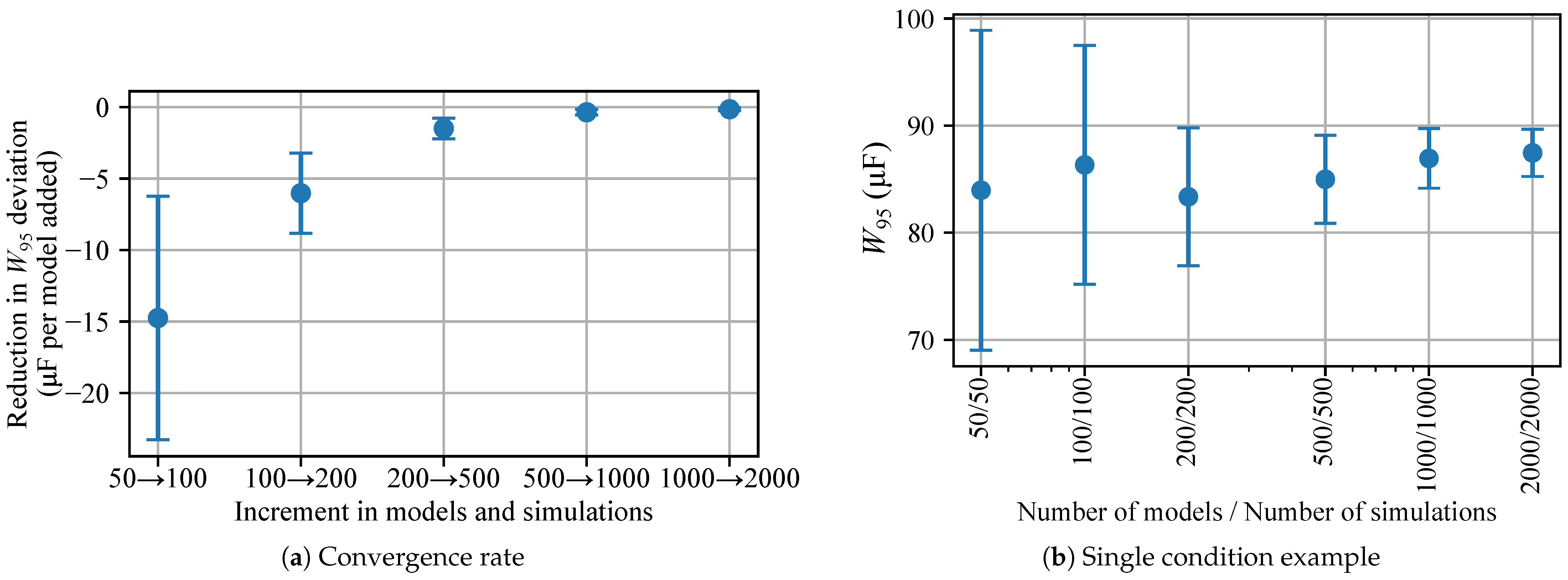
A convergence analysis was employed to choose a sufficient number of models and simulations for the MCSs. For this analysis, the same number of models and simulations was considered, and 50 iterations of the proposed method were performed for combinations ranging from 50 to 2000 models and simulations. Figure 2a presents an evaluation of the reduction in variation from increasing the number of MCSs, which shows little gain after increasing the model size to 500, and negligible gain from increasing the model size from 1000 to 2000 models and simulations. Figure 2b presents an example of single-condition analysis, in which this diminishing return can also be seen. Since a similar result was observed for all three MLP architectures, a value of 1000 models and simulations was chosen for the uncertainty ensemble.

Figure 2. Convergence evaluation for the trilayered architecture. (a) Convergence of the deviation in the confidence interval for increasing number of models and simulations. (b) Convergence analysis for a single test condition.

Table 4 provides numeric results of the inference errors and the width of the confidence interval obtained with the proposed method. To better understand the results of each model under specific conditions of the test data, the results are separated into global performance and a subset for each capacitance value. In terms of mean absolute error (MAE) and root mean squared error (RMSE), the trilayered architecture achieved the lowest estimation error, whereas the medium architecture showed a marginal increase in error, and the wide model yielded the highest error rates. Compared with the original study, which reported maximum experimental MAE and RMSE of $6.23$ $\mathsf{\mu }$$\mathrm{F}$ and $7.94$ $\mathsf{\mu }$$\mathrm{F}$, respectively, the errors obtained in the proposed frequency-converter drive setup were higher. This increase can be attributed to the more demanding operating conditions of the present setup, including higher power levels and larger capacitance values, the use of a dynamic motor load instead of the static resistive and resistive-inductive loads considered in the original study, and the evaluation over multiple inverter output frequencies rather than a single operating frequency.

Table 4. Performance metrics separated by capacitance value.

Architecture	Value	MAE ( $\mathsf{\mu }$$\mathbf{F}$)	RMSE ( $\mathsf{\mu }$$\mathbf{F}$)	Interval Width (95%, $\mathsf{\mu }$$\mathbf{F}$)
Trilayered	Global	44.26	55.30	44.44
Trilayered	777 $\mathsf{\mu }$$\mathrm{F}$	56.17	66.14	48.23
Trilayered	919 $\mathsf{\mu }$$\mathrm{F}$	32.35	41.74	40.64
Medium	Global	49.20	60.02	56.81
Medium	777 $\mathsf{\mu }$$\mathrm{F}$	58.27	69.76	61.20
Medium	919 $\mathsf{\mu }$$\mathrm{F}$	40.13	48.35	52.42
Wide	Global	67.69	77.84	12.97
Wide	777 $\mathsf{\mu }$$\mathrm{F}$	79.78	91.10	13.56
Wide	919 $\mathsf{\mu }$$\mathrm{F}$	55.59	61.80	12.38

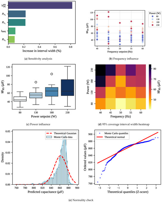
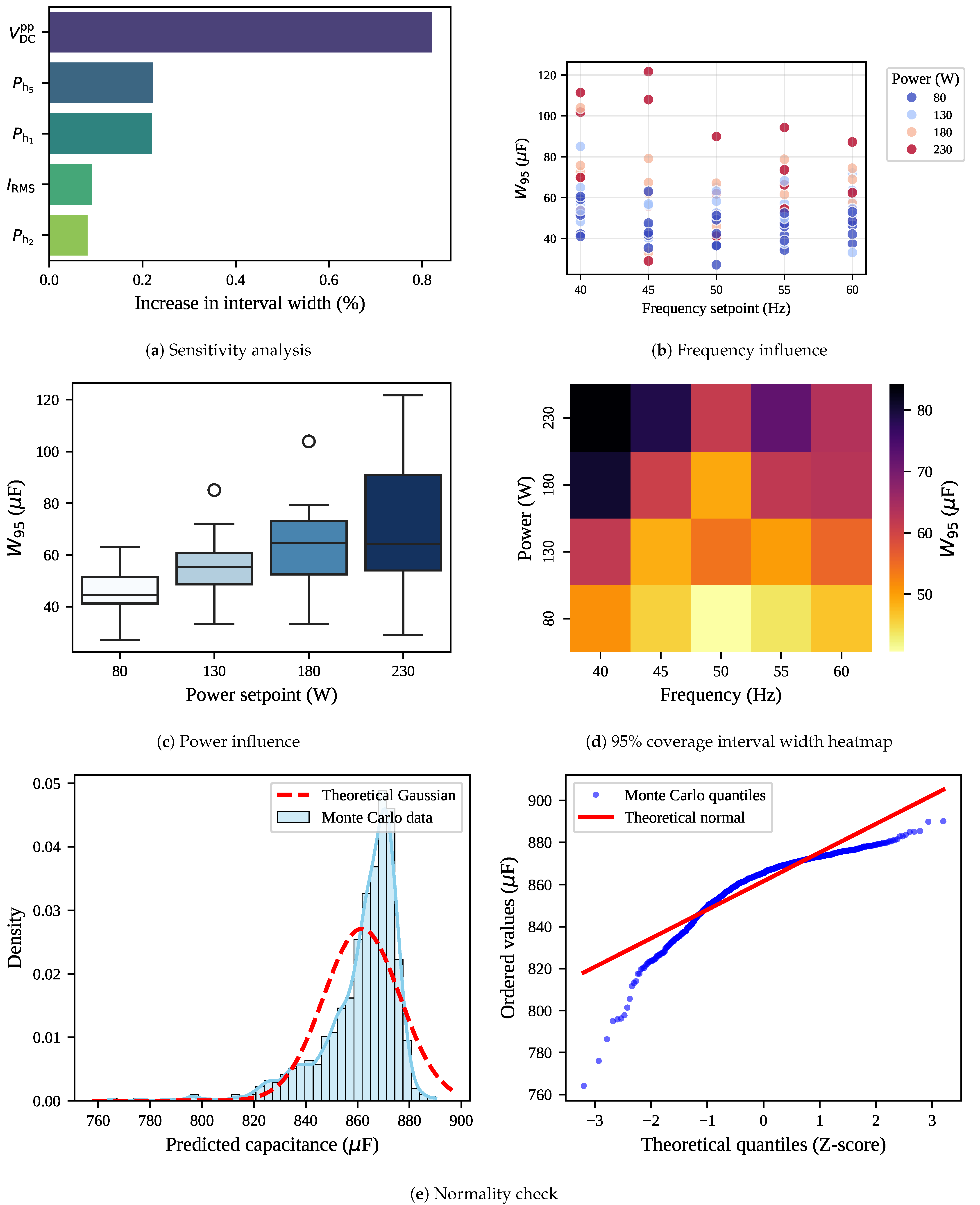
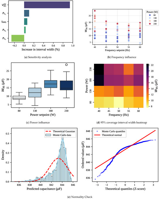
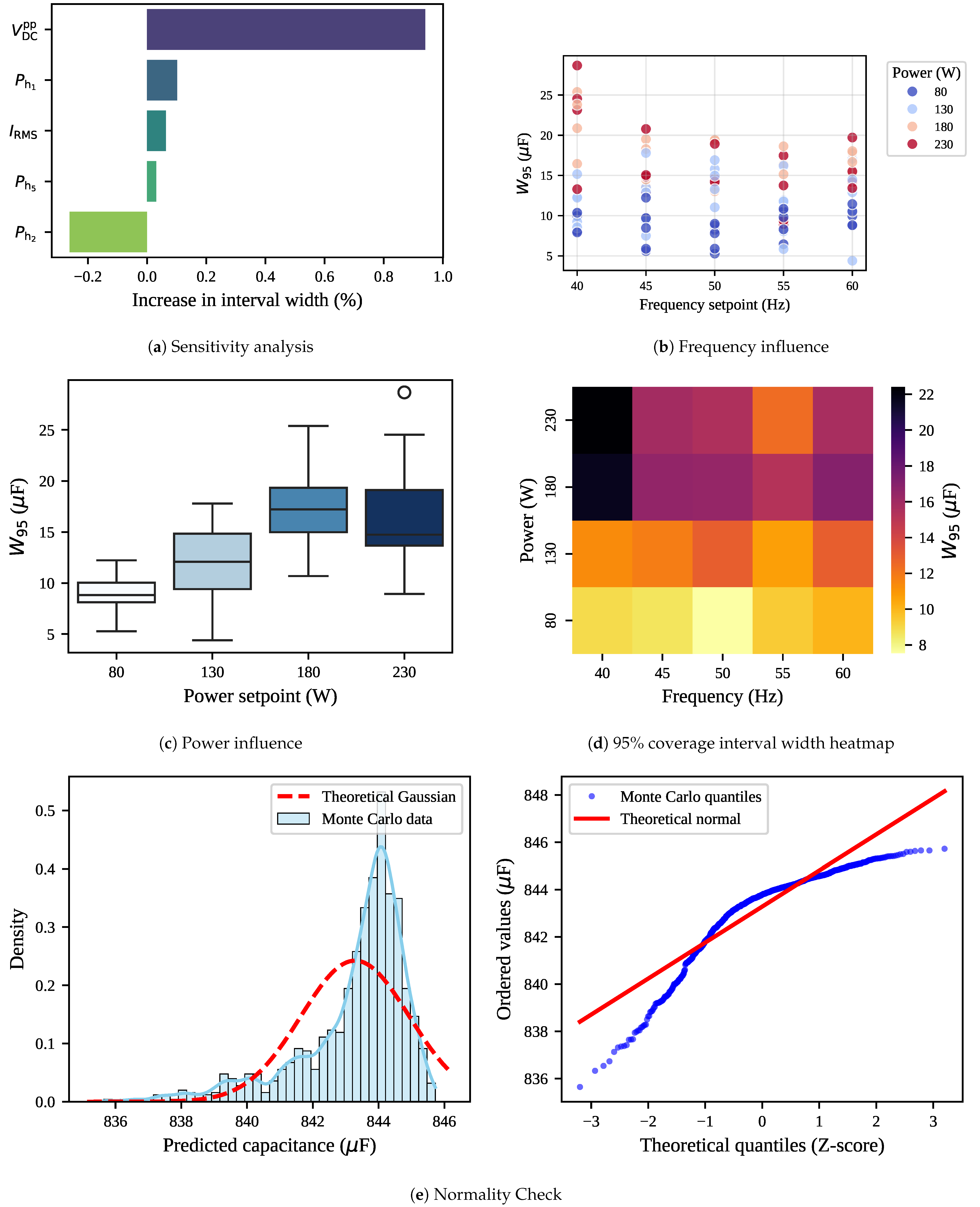
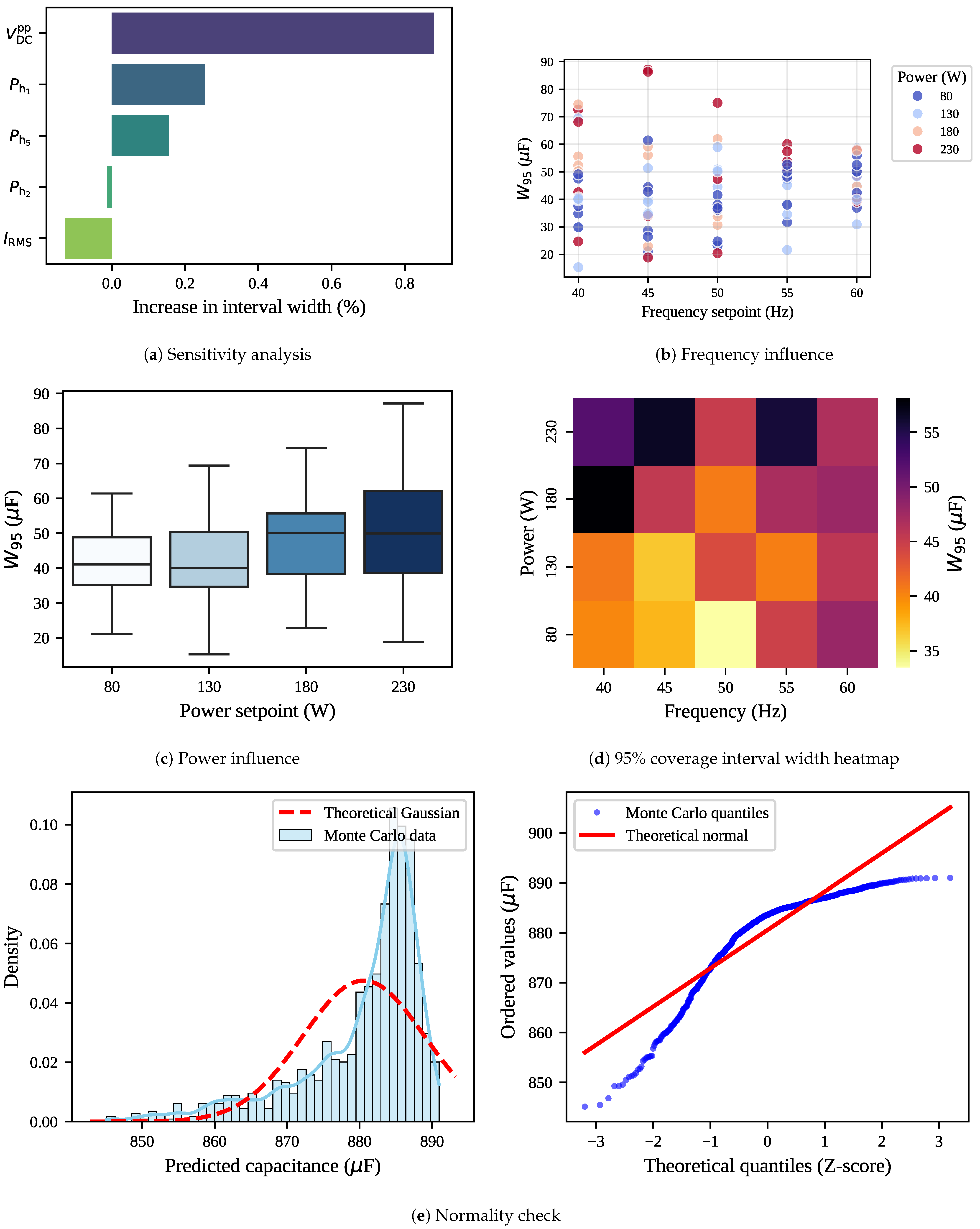
Regarding uncertainty, the mean interval width (denoted as $W_{95}$ in Figure 3, Figure 4 and Figure 5) is computed for a coverage probability of 95%. It is important to note that this width is computed dynamically: for samples showing Gaussian behavior, it corresponds to twice the analytical expanded uncertainty ($2·k·u_{\mathrm{c}}$); for non-Gaussian distributions, it is derived numerically from the span between the 2.5th and 97.5th percentiles.

Figure 3. Results for the medium architecture. (a) Sensitivity ranking of input features regarding interval width. (b) Influence of frequency on uncertainty. (c) Influence of power on uncertainty. (d) Uncertainty heatmap across the operational range. (e) Statistical normality test for the most non-Gaussian sample.

Figure 4. Results for the wide architecture. (a) Sensitivity ranking of input features regarding interval width. (b) Influence of frequency on uncertainty. (c) Influence of power on uncertainty. (d) Uncertainty heatmap across the operational range. (e) Statistical normality test for the most non-Gaussian sample.

Figure 5. Results for the trilayered architecture. (a) Sensitivity ranking of input features regarding interval width. (b) Influence of frequency on uncertainty. (c) Influence of power on uncertainty. (d) Uncertainty heatmap across the operational range. (e) Statistical normality test for the most non-Gaussian sample.

Increasing the number of hidden neurons from 25 to 100 degraded the overall performance. The wide architecture exhibited the highest estimation errors alongside the narrowest confidence intervals (i.e., highest confidence). This overconfidence, combined with high test error, suggests that the wide model is overly complex for the available dataset, leading to overfitting and poor generalization. Conversely, the medium architecture proved to be the most conservative, producing the widest uncertainty bounds while maintaining lower errors than the wide model. Finally, the trilayered architecture achieved the best overall balance in terms of error, yielding the lowest overall estimation error coupled with a mid-range uncertainty interval.

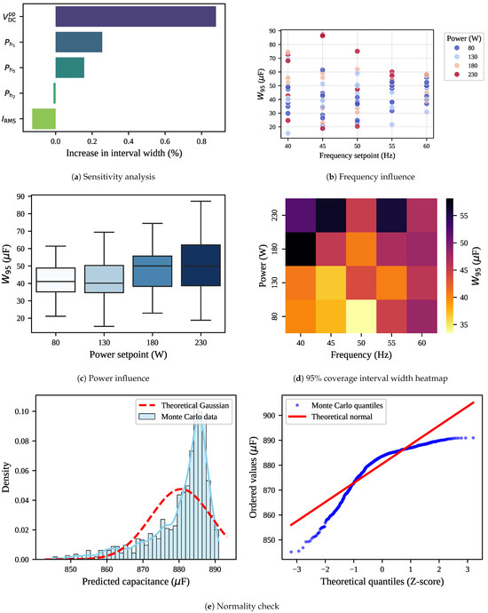
Further metrological analyses are shown in Figure 3, Figure 4 and Figure 5 for the medium, wide, and trilayered architectures, respectively. Figure 3a, Figure 4a and Figure 5a show tests increasing the uncertainty of one input variable at a time by 1%, indicating that the peak-to-peak voltage of the DC link is the variable that has the most influence over the final coverage interval width, as the output varies upwards to 0.82% when its uncertainty is increased, outweighing all other features. From a physical perspective, this is consistent with the role of capacitors in filtering voltage fluctuations; therefore, the estimation of capacitance is inherently tied to the dynamic relationship between voltage ripple and current. Plots regarding the operating point, such as scatter plots indicating the frequency (Figure 3b, Figure 4b and Figure 5b) and bar plots indicating power influence–Figure 3c, Figure 4c and Figure 5c–of the baseline data, also show that frequency does not have much of an influence on the 95% uncertainty of the models, while the power shows a slight trend of higher uncertainty with higher power setpoints. Lastly, Figure 3d, Figure 4d and Figure 5d indicate heatmaps colored by the average confidence interval with both frequency and power setpoints that suggest that higher power tends to have higher uncertainty. From a physical perspective, higher power operation requires larger load currents, which cause deeper discharges of the DC-link capacitor between rectifier cycles. This dynamic leads to a larger voltage ripple magnitude and an increase in the complexity of the harmonic content. Consequently, the input features extracted under these conditions become more volatile, amplifying the measurement uncertainty propagated through the models.

Additionally, Figure 3e, Figure 4e and Figure 5e illustrate the model distribution for the most non-Gaussian sample for each model. This distribution corresponds to a 919 $\mathsf{\mu }$$\mathrm{F}$ capacitor operating at 80 $\mathrm{W}$ and 50 $\mathrm{Hz}$ for the wide structure and at 230 $\mathrm{W}$ and 55 $\mathrm{Hz}$ for the medium and trilayered architectures. The histogram constructed uses ${10}^6$ MCS propagated through the uncertainty ensemble. The visual discrepancy between the empirical histogram and the theoretical Gaussian fit can be confirmed through the Quantile-Quantile (Q-Q) plot, where the empirical quantiles (blue dots) deviate significantly from the theoretical Gaussian reference (red line).

Interestingly, the depth of the architecture influenced the shape of the uncertainty distribution. All models consistently exhibited negative skewness and positive kurtosis, characteristic of asymmetric, leptokurtic distributions with sharp peaks and heavy left tails. However, the shallower and narrower medium architecture presented the most extreme distortion, reaching a high kurtosis of $5.36$ and a skewness of $-1.86$. In contrast, increasing the network capacity, either through width (wide architecture, kurtosis of $2.58$) or depth (trilayered architecture, kurtosis of $2.33$), attenuated this extreme sharp-peaking effect, resulting in slightly more dispersed probability density functions. Despite this attenuation, the persistent leptokurtic and left-skewed behavior across all architectures mathematically validates the necessity of the proposed hybrid Anderson–Darling approach, as relying on traditional Gaussian assumptions would fail to capture these heavy tails.

To validate the choice of the nonparametric uncertainty estimation method, a comprehensive normality test was performed on the entire test set (100 samples). The Anderson–Darling test rejected the null hypothesis of normality for the vast majority of the predictions, confirming the heavy-tailed nature of the propagated measurement noise. At a 5% significance level (critical value of $0.784$), the rejection rates were 87% for the wide architecture, 91% for the medium architecture, and 94% for the trilayered architecture. Notably, for the trilayered model, the test statistics ranged from 0.25 up to 54.95, significantly exceeding the critical value in most operational scenarios. These empirical findings conclusively demonstrate that relying strictly on traditional Gaussian-based assumptions would systematically fail to capture the uncertainty bounds in this application, thereby validating the necessity of the proposed adaptive and nonparametric approach.

Compared to existing approaches in the literature, the proposed method offers an advantage by not only estimating the capacitor health indicators but also quantifying the uncertainties inherent to the measurement process. While recent data-driven methods achieve very low estimation errors, they typically only provide singular point estimates. Such outputs lack the reliability bounds required for industrial maintenance decision-making. In contrast, the proposed method returns, along with the prediction, a confidence interval to its result. Furthermore, this framework operates on easily obtainable operational signals, reducing implementation complexity and costs.

Despite these advantages, the practical application boundaries of the proposed framework must be acknowledged. First, regarding computational and real-time requirements, it is important to emphasize that the proposed method is specifically designed for offline condition monitoring. While propagating Monte Carlo samples through an ensemble of 1000 neural networks imposes a significant computational load, real-time execution is not required for end-of-life assessment, making this load practically manageable. Second, the framework is inherently sensitive to the training data size; the baseline dataset must be sufficiently large and diverse to ensure that the bootstrap resampling and subsequent out-of-bag validation can effectively filter out poorly converged models. Finally, as demonstrated by the evaluation of the wide architecture earlier in this section, the reliability of the method is bounded by model complexity. If an overly complex estimator is employed, the framework naturally exposes this limitation by revealing severe overfitting through high estimation errors and unreliably narrow confidence intervals, thereby acting as a diagnostic boundary for the user.

5. Conclusions

This paper presents a method that can be used for the metrological evaluation of state-of-the-art data-driven soft sensors designed for health monitoring of capacitors in the DC link of power converters. The proposed method is based on Monte Carlo simulations combined with bootstrapping and was validated in a case study that used a recent method from the literature for the online estimation of DC-link capacitance in frequency converters. In this case study, it was possible to propagate the uncertainty from the power analyzer measurements used to measure the input features of the artificial neural network models for the inference of capacitance in order to obtain an estimate of the confidence interval of the inferences.

The sensitivity analysis of the case study identified the peak-to-peak DC-link voltage as the most critical input variable, indicating that instrumentation efforts should focus on the acquisition of the voltage ripple with low uncertainty values. Furthermore, the combination of non-Gaussian input distributions and the nonlinear behavior of the process tends to produce non-Gaussian distributions of the capacitance. This suggests that the proposed method to address this characteristic is necessary to ensure reliable confidence intervals for the predictions.

Future work will focus on evaluating the proposed uncertainty assessment method alongside other data-driven capacitance and series resistance methods to determine not only the methods that provide smaller errors for a test dataset but also those that yield smaller confidence intervals. Additionally, further studies will be done to evaluate the proposed method in different conditions, including both model parameters, such as training data size and model complexity, as well as experimental test parameters, such as motor power and load condition.

References

- Joddumahanthi, V.; Knypiński, Ł; Gopal, Y.; Kasprzak, K. Review of Power Electronics Technologies in the Integration of Renewable Energy Systems. Appl. Sci. 2025, 15, 4523. [Google Scholar] [CrossRef] [Scilit]
- Diaz, M.; Rojas, A.; Rodríguez, J. Power Electronics for Energy Transition and Renewable Energy Conversion Processes. Processes 2025, 13, 3650. [Google Scholar] [CrossRef] [Scilit]
- Tang, Z.; Yang, Y.; Blaabjerg, F. Power electronics: The enabling technology for renewable energy integration. CSEE J. Power Energy Syst. 2022, 8, 39–52. [Google Scholar] [CrossRef] [Scilit]
- Cai, Z.; Huang, J.; Huang, X.; Li, Y.; Xiong, W.; Tang, Z.; Liang, B. An Efficient Power Management Circuit for Battery Monitoring Systems. In Proceedings of the 2024 4th International Conference on Electronic Information Engineering and Computer Communication (EIECC), Wuhan, China, 27–29 December 2024; pp. 204–208. [Google Scholar] [CrossRef] [Scilit]
- Monadi, M.; Nabipour, M.; Akbari-Behbahani, F.; Pouresmaeil, E. Speed Control Techniques for Permanent Magnet Synchronous Motors in Electric Vehicle Applications Toward Sustainable Energy Mobility: A Review. IEEE Access 2024, 12, 119615–119632. [Google Scholar] [CrossRef] [Scilit]
- Rihar, A.; Nemec, M.; Lavrič, H.; Zajec, P.; Vončina, D.; Nedeljković, D.; Ambrožič, V.; Drobnič, K. Emerging Technologies for Advanced Power Electronics and Machine Design in Electric Drives. Appl. Sci. 2024, 14, 11559. [Google Scholar] [CrossRef] [Scilit]
- Rosas, E.; Bórquez, C.; Barria, D.; Ojeda, S.; Rohten, J.; Silva, J. Comparison of Control Strategies for Induction Motors: Indirect Field Oriented Control, Direct Torque Control and Predictive Torque Control. In Proceedings of the 2024 IEEE International Conference on Automation/XXVI Congress of the Chilean Association of Automatic Control (ICA-ACCA), Santiago, Chile, 20–23 October 2024; pp. 1–6. [Google Scholar] [CrossRef] [Scilit]
- Alshammari, S.; Alharbi, M.; Burugula, V.; Alosaimi, H.; Aladhyani, H.; Bhattacharya, S. Modular Multilevel Converter (MMC) Based Direct Tapping Method for High Voltage DC Transmission Networks. In Proceedings of the 2024 IEEE Energy Conversion Congress and Exposition (ECCE), Phoenix, AZ, USA, 20–24 October 2024; pp. 240–246. [Google Scholar] [CrossRef] [Scilit]
- Caramori, M.M.; Dall’Asta, M.S.; dos Santos, I.L.; Mezaroba, M.N.; Pacheco, A.L.S.; Didjurgeit, M.; Mussa, S.A.; Lazzarin, T.B. Study, Design and Implementation of a Single-Phase Double-Conversion Online Transformerless Uninterruptible Power Supply Prototype. In Proceedings of the 2025 Brazilian Power Electronics Conference (COBEP), Vitoria, Brazil, 5–8 October 2025; pp. 1–5. [Google Scholar] [CrossRef] [Scilit]
- Das, R.; Le, H.P. Two-Stage Power Delivery Architecture Using Hybrid Converters for Data Centers and Telecommunication Systems. Electronics 2025, 14, 3169. [Google Scholar] [CrossRef] [Scilit]
- Gasperi, M. Life prediction modeling of bus capacitors in AC variable-frequency drives. IEEE Trans. Ind. Appl. 2005, 41, 1430–1435. [Google Scholar] [CrossRef]
- Falck, J.; Felgemacher, C.; Rojko, A.; Liserre, M.; Zacharias, P. Reliability of Power Electronic Systems: An Industry Perspective. IEEE Ind. Electron. Mag. 2018, 12, 24–35. [Google Scholar] [CrossRef] [Scilit]
- Torki, J.; Joubert, C.; Sari, A. Electrolytic capacitor: Properties and operation. J. Energy Storage 2023, 58, 106330. [Google Scholar] [CrossRef] [Scilit]
- Kim, Y.T.; Kim, K.B.; Hyun, Y.E.; Kim, I.J.; Yang, S. Simulation study on the lifetime of electrochemical capacitors using the accelerated degradation test under temperature and voltage stresses. Microelectron. Reliab. 2015, 55, 2712–2720. [Google Scholar] [CrossRef] [Scilit]
- Saravanakumar, R.; Sivakumar, N.; Devi, V.S.K.; Shanthini, C.; Debashisha, J.; Ibaceta, E.; Diaz, M.; Rodriguez, J. Condition Monitoring of Submodule Capacitors in Modular Multilevel Converters—A Review. J. Energy Storage 2025, 134, 117954. [Google Scholar] [CrossRef] [Scilit]
- Liu, C.; Deng, F.; Yu, Q.; Wang, Y.; Blaabjerg, F.; Cai, X. Submodule Capacitance Monitoring Strategy for Phase-Shifted Carrier Pulsewidth-Modulation-Based Modular Multilevel Converters. IEEE Trans. Ind. Electron. 2021, 68, 8753–8767. [Google Scholar] [CrossRef] [Scilit]
- Xiao, Q.; Wang, H.; Jin, Y.; Jia, H.; Mu, Y.; Zhu, J.; Teodorescu, R.; Blaabjerg, F. Submodule Capacitance Monitoring Approach for the MMC With Asymptotically Converged Error. IEEE Trans. Ind. Electron. 2024, 71, 4330–4339. [Google Scholar] [CrossRef] [Scilit]
- Jiang, H.; Deng, F.; Li, H.; Tian, J.; Lu, Y.; Li, G. A Capacitance Monitoring Strategy Based on Offset Error Compensation for Modular Multilevel Converters. Energies 2024, 17, 1771. [Google Scholar] [CrossRef] [Scilit]
- Roh, C.; Jeon, H.m.; Kim, S.w.; Kim, J.s.; Song, S.w.; Lee, N.y.; Kang, S.c. A Study on Equivalent Series Resistance Estimation Compensation for DC-Link Capacitor Life Diagnosis of Propulsion Drive in Electric Propulsion Ship. Processes 2025, 13, 291. [Google Scholar] [CrossRef] [Scilit]
- Xia, H.; Zhang, Y.; Wang, H.; Chen, M.; Lai, W.; Luo, D.; Hu, Y. Condition Monitoring for Capacitors in Modular Multilevel Converter Based on High-frequency Transient Analysis. In Proceedings of the 2021 IEEE Energy Conversion Congress and Exposition (ECCE), Virtual, 10–14 October 2021; pp. 5342–5347. [Google Scholar] [CrossRef] [Scilit]
- Zhao, Z.; Lu, W.; Davari, P.; Du, X.; Iu, H.H.C.; Blaabjerg, F. An Online Parameters Monitoring Method for Output Capacitor of Buck Converter Based on Large-Signal Load Transient Trajectory Analysis. IEEE J. Emerg. Sel. Top. Power Electron. 2021, 9, 4004–4015. [Google Scholar] [CrossRef] [Scilit]
- Xia, H.; Zhang, Y.; Chen, M.; Lai, W.; Luo, D.; Wang, H. Capacitor Condition Monitoring for Modular Multilevel Converter Based on Charging Transient Voltage Analysis. IEEE Trans. Power Electron. 2023, 38, 3847–3856. [Google Scholar] [CrossRef] [Scilit]
- Shahraki, A.F.; Al-Dahidi, S.; Taleqani, A.R.; Yadav, O.P. Using LSTM Neural Network to Predict Remaining Useful Life of Electrolytic Capacitors in Dynamic Operating Conditions. Proc. Inst. Mech. Eng. Part O J. Risk Reliab. 2022, 237, 16–28. [Google Scholar] [CrossRef] [Scilit]
- Liu, H.; Claeys, T.; Pissoort, D.; Vandenbosch, G.A.E. Long-Term Prediction of Multistress Accelerated Aging of Capacitors by Long Short-Term Memory Network. IEEE Trans. Instrum. Meas. 2023, 72, 1009106. [Google Scholar] [CrossRef] [Scilit]
- de Andrade, M.A.; Flesch, R.C.C. Capacitance Estimation Algorithm for Condition Monitoring of Electrolytic DC-Link Capacitors Using Artificial Neural Network in Front-End Diode Rectifier Three-Phase Motor Drive Systems. In Proceedings of the 2023 IEEE 8th Southern Power Electronics Conference, Florianopolis, Brazil, 26–29 November 2023; pp. 1–7. [Google Scholar] [CrossRef] [Scilit]
- AL-Wesabi, I.; Al-Shamma’a, A.A.; Hussein Farh, H.M.; Dawood, R.A.; Mwakipunda, G.C.; Xu, J. Capacitance Estimation Algorithm Based on DC-link Voltage Ripples Using Hybrid Machine Learning Techniques in Power Electronics Converters. Results Eng. 2025, 27, 106216. [Google Scholar] [CrossRef] [Scilit]
- Behrooz, A.; Soleimanifar, A.; Zolghadri, M.R. Regression-Based Machine Learning Approaches for Capacitor Condition Monitoring in Boost PFC Converter. In Proceedings of the 2025 16th Power Electronics, Drive Systems, and Technologies Conference (PEDSTC), Tabriz, Iran, 4–6 February 2025; pp. 1–5. [Google Scholar] [CrossRef] [Scilit]
- Örüklü, K.; Ağalar, Ş. Machine Learning-Based Condition Monitoring for DC-Link Capacitors in AC/DC/AC Converters. IEEE Trans. Ind. Electron. 2025, 72, 4227–4237. [Google Scholar] [CrossRef] [Scilit]
- Miao, W.; Lam, K.H.; Pong, P.W.T. Online Monitoring of Aluminum Electrolytic Capacitors in Photovoltaic Systems by Magnetoresistive Sensors. IEEE Sens. J. 2020, 20, 767–777. [Google Scholar] [CrossRef] [Scilit]
- Yao, B.; Wei, X.; Zhang, Y.; Lin, Z.; Wang, H.; Wang, H. Remaining Useful Life Prediction of Aluminum Electrolytic Capacitor with a Strain-based Health Indicator. In Proceedings of the 2024 IEEE Applied Power Electronics Conference and Exposition (APEC), Long Beach, CA, USA, 25–29 February 2024; pp. 2438–2442. [Google Scholar] [CrossRef] [Scilit]
- Nisar, S.; Barbará, P.V.; Chachuat, B.; Hallett, J.P.; Brandt-Talbot, A. Near-infrared spectroscopy for rapid compositional analysis of cellulose pulps after fractionation with ionic liquids. Biomass Bioenergy 2025, 201, 108056. [Google Scholar] [CrossRef] [Scilit]
- Schiering, N.; Eichstädt, S.; Heizmann, M.; Koch, W.; Schneider, L.S.; Scheele, S.; Sommer, K.D. Modelling of measuring systems—From white box models to cognitive approaches. Meas. Sens. 2025, 38, 101503. [Google Scholar] [CrossRef] [Scilit]
- Bublil, T.; Cohen, R.; Kenett, R.S.; Bortman, J. Machine Health Indicators and Digital Twins. Sensors 2025, 25, 2246. [Google Scholar] [CrossRef] [Scilit]
- Diniz, F.; Pinto, T.; Matos, S.; Luz, E.; Pessin, G.; Ueyama, J. Enhancing Operational Safety with Conformal Prediction in Soft Sensors. Proc. IFAC 2025, 59, 84–89. [Google Scholar] [CrossRef] [Scilit]
- Thaler, G.; Machado, J.P.Z.; Flesch, R.C.C.; Pacheco, A.L.S. Metrologically Interpretable Soft-Sensing Technique for Non-Invasive Liquid Flow Estimation from Vibration Data. Metrology 2025, 5, 6. [Google Scholar] [CrossRef] [Scilit]
- Lee, H.S.; Park, S.H.; Kim, S.Y. Cost-Efficient Sensing With Self-Improving Soft Sensor Based on Predictive Uncertainty Estimation in IoT Environments. IEEE Internet Things J. 2026, 13, 3055–3068. [Google Scholar] [CrossRef] [Scilit]
- Morales, H.; Aguirre-Zapata, E.; Shi, X.; Sciascio, F.d.; Amicarelli, A.N. A Bayesian Gaussian Process Regression soft sensor for industrial sugar crystallization monitoring. J. Food Eng. 2026, 412, 112990. [Google Scholar] [CrossRef] [Scilit]
- Wang, Z.; Bu, S.; Wen, J.; Huang, C. A comprehensive review on uncertainty modeling methods in modern power systems. Int. J. Electr. Power Energy Syst. 2025, 166, 110534. [Google Scholar] [CrossRef] [Scilit]
- Song, Y.; Schirmer, P.A.; Schreivogel, P.; Zhang, K.; Wang, H.; Blaabjerg, F. On the Sensitivity Analysis in Reliability Evaluation for Power Electronic Converters. IEEE Trans. Power Electron. 2025, 40, 7251–7260. [Google Scholar] [CrossRef] [Scilit]
- Lv, C.; Liu, J.; Zhang, Y. A data-driven method for anomaly detection and aging model parameter estimation of capacitors based on condition monitoring. Microelectron. Reliab. 2022, 138, 114646. [Google Scholar] [CrossRef] [Scilit]
- Gawlikowski, J.; Tassi, C.R.N.; Ali, M.; Lee, J.; Humt, M.; Feng, J.; Kruspe, A.; Triebel, R.; Jung, P.; Roscher, R.; et al. A survey of uncertainty in deep neural networks. Artif. Intell. Rev. 2023, 56, 1513–1589. [Google Scholar] [CrossRef] [Scilit]
- Pacheco, A.L.; Flesch, R.C.; Flesch, C.A.; Iervolino, L.A.; Barros, V.T. Tool based on artificial neural networks to obtain cooling capacity of hermetic compressors through tests performed in production lines. Expert Syst. Appl. 2022, 194, 116494. [Google Scholar] [CrossRef] [Scilit]
- BIPM; IEC; IFCC; ILAC; ISO; IUPAC; IUPAP; OIML. JCGM 101:2008; Evaluation of Measurement Data—Supplement 1 to the “Guide to the Expression of Uncertainty in Measurement”—Propagation of Distributions Using a Monte Carlo Method. Joint Committee for Guides in Metrology: Sèvres, France, 2008. [CrossRef] [Scilit]
- JJCGM 100:2008; Evaluation of Measurement Data—Guide to the Expression of Uncertainty in Measurement. International Organization for Standardization: Geneva, Switzerland, 2008.
- Anderson–Darling Test. In The Concise Encyclopedia of Statistics; Springer: New York, NY, USA, 2008; pp. 12–14. [CrossRef] [Scilit]
- Yokogawa Electric Corporation. PZ4000 Power Analyzer: User’s Manual; Version PIM 103-03E; Yokogawa Electric Corporation: Tokyo, Japan, 2009. [Google Scholar]
Disclaimer/Publisher’s Note: The statements, opinions and data contained in all publications are solely those of the individual author(s) and contributor(s) and not of MDPI and/or the editor(s). MDPI and/or the editor(s) disclaim responsibility for any injury to people or property resulting from any ideas, methods, instructions or products referred to in the content. |
© 2026 by the authors. Licensee MDPI, Basel, Switzerland. This article is an open access article distributed under the terms and conditions of the Creative Commons Attribution (CC BY) license.