


Abstract
In pressurized irrigation networks, water-intake hydrants combine flow regulation, shutoff and metering in a single cast body, and the resulting coupled resistance obscures how much each function costs. The conventional body of a DN100 (nominal diameter 100 mm) hydrant and a redesigned production variant were solved with an incompressible Reynolds-averaged Navier–Stokes (RANS) model in three functional configurations (bare body, +regulator, +metering line) at five inlet velocities (1–5 m s−1, Re ≈ 1.0 × 10⁵–5.0 × 10⁵). The mesh was selected after a four-level refinement study, and the quarter-symmetry assumption was verified against two full-domain calculations with both symmetry planes removed: the reduced domain costs 1.0% in pressure drop, and the transverse forces and the net moment on the regulator vanish in the time mean, leaving the axial thrust as the only physically meaningful regulator load. The redesigned body lowers the bare-body loss coefficient by 30.9% and raises Kv by 20.3%. Adding the regulator removes that advantage—ξ becomes 3.0% worse and the full-device axial thrust 11.9% higher—and adding the metering line widens the gap to 37.0% in loss and 60.8% in thrust. Loss and mechanical load therefore reverse sign together at integration, so a body improvement demonstrated in isolation cannot be assumed to survive assembly. The decomposition also acted as a consistency check: a negative metering-line increment in the conventional device, impossible for a passive addition, was traced to a 23.5% passage enlargement present in the supplied full-device geometry rather than to the flow. Wall data give a minimum static pressure of 0.20 bar and a local cavitation number of 1.39, a margin five times narrower than a lumped estimate suggests. Flow-bench measurements on the finished product provide an independent order-of-magnitude reference rather than a validation. The configuration-additive decomposition and the axial-thrust indicator together form an evaluation approach transferable to other devices that combine sub-functions in one body, subject to confirmation on further geometries and Reynolds ranges.
1. Introduction
In pressurized closed irrigation networks, the distribution of water to each field is carried out through water-intake hydrants (irrigation hydrants). Although network-level distribution-line design and sustainable operating parameters [1], demand-based outlet behavior [2], and the effect of irrigation management on infiltration [3] have been studied extensively, the internal hydraulics of the hydrant, the device at the node of these networks, has received less attention. A modern hydrant combines, in a single ductile-iron (GGG40) body, a flow regulator that provides a constant flow rate to the field even when the upstream pressure fluctuates, a diaphragm mechanism for shutoff, and a flow-metering line for billing. This functional concentration simplifies assembly. However, the sudden cross-sectional changes, side chambers, and regulator element inside the body produce turbulent separation and secondary flows. This in turn causes a measurable head loss and directly increases the network pumping energy.
The investigation of valve and regulator geometries by computational fluid dynamics (CFD) is a mature field. The stabilization of the flow field in irrigation regulators [4], a review of pipeline pressure-regulation technologies [5], the spring- and structure-based multi-step optimization of a side-inlet pressure regulator [6], compressible turbulent flow in a multistage high-pressure-reducing valve [7], the CFD determination of the flow coefficient in a proportional control valve [8], the CFD analysis of flow parameters in an agricultural mini valve [9], and flow modeling in pneumatic valves [10] are representative examples of this literature. The common point is that, for the most part, a single hydraulic element (only the valve or only the regulator) is treated in isolation.
A parallel and largely separate literature examines the accuracy of flow metering under distorted velocity profiles. The sensitivity of Woltmann meters to flow disturbances [11], the accuracy of an in-pipe metering device in a sandy water source [12], a multi-parameter smart metering device for urban flow measurement [13], guidelines for clamp-on ultrasonic metering [14], the flow patterns inside an ultrasonic meter [15], two-station ultrasonic meters over a wide dynamic range [16], the swirl decay rate in turbulent pipe flow [17], flow-conditioner efficiency [18], and the CFD assessment of installation effects [19] are the main contributions along this axis. These studies show that metering accuracy depends critically on the upstream geometry. However, they do not treat the regulator/body geometry feeding the measurement line together with the metering region in a single flow field. Beyond single elements, a smaller body of work has begun to address devices that combine several hydraulic stages or functions in a single body. The flow characteristics distributed over the successive throttling stages of a multistage sleeve control valve have been solved numerically [20], and the individual contributions of the throttling cone, body, and deflector to the internal field of a pressure-reducing valve have been decomposed on a component basis [21]. These studies show that the sub-components in a multi-function body interact hydraulically and that the overall response cannot be inferred from any single element treated in isolation. An integrated irrigation hydrant combining regulation, shutoff, and metering, however, has not yet been decomposed in this way.
In the author’s previous work, the three-dimensional flow during the opening process of a single-disc butterfly valve was investigated with a moving-mesh approach, and conventional and optimized disc geometries were compared [22]. The redesigned body evaluated in this study is based on a corrugated (stress-distributing) body structure [23]. The drag-based optimization of the regulator/disc element [24] and geometry-based optimization in cast hydraulic components [25] are related preceding works. This numerical and applied background forms the basis of the present study.
Where the hydrant itself appears in this literature, it appears as a node rather than as a device. Fouial et al. [26] generate configurations of simultaneously operating hydrants for a 74-hydrant district and analyze them in EPANET under demand-driven and pressure-driven formulations, with each hydrant reduced to a nominal discharge and a minimum guaranteed head of 20 m; the internal geometry that produces that head requirement is never resolved. The devices whose internal flow has actually been computed are single-function valves. Yang et al. [27] solved a hydraulically driven irrigation control valve of DN160 inlet and DN90 outlets with a standard k–ε closure on 1.22 × 10⁶ cells and a moving spool, obtaining a flow coefficient Kv = 79.26 and a resistance coefficient of 16.70 against laboratory measurements that agreed to within 6–9%. Yu et al. [28] computed a diaphragm valve of 110.5 mm bore in OpenFOAM, compared five Reynolds-averaged Navier–Stokes (RANS) closures with manufacturer pressure-drop data, and found the resistance coefficient to fall from 7.51 to 7.11 as Re rose from 0.4 × 10⁵ to 4.8 × 10⁵, the shear-stress transport (SST) k–ω model deviating by 0.29–2.43% and the Spalart–Allmaras model by up to 18.42%. The two studies do not agree on closure, one defending a k–ε family for a spool valve and the other a k–ω family for a diaphragm, which is itself a reason to state the turbulence treatment and its verification explicitly rather than by reference. Multi-function devices, in contrast, have been characterized experimentally and from the outside: Liu et al. [29] built and calibrated a body combining regulation and measurement, reporting Kv = 84.61 and a flow-measurement error within 3% but no flow field, and Bijankhan et al. [30] tested a constant-flow control valve in the laboratory and in the field, recovering 23.5–28% of otherwise lost water, again without resolving the internal flow. What the literature supplies is therefore the resistance of single elements computed in isolation and the performance of integrated devices measured from outside. Neither states how much of an integrated hydrant’s resistance belongs to the body, to the regulator or to the metering line, which is the quantity a designer needs before deciding where material and machining should go.
The gap in the literature becomes clear at the following points: (i) an integrated hydrant combining the regulation, shutoff, and metering functions has not been investigated by CFD with the contribution of the sub-functions to the loss decomposed, (ii) the hydraulic force and moment on the regulator element are rarely reported as a design performance indicator (KPI), and (iii) the net hydraulic benefit of a body optimization has not been tracked with the sub-component integration taken into account. To the author’s knowledge, there is no previous CFD study that combines the additive decomposition of an integrated regulation-shutoff-metering hydrant with reporting the regulator hydraulic load as a design indicator, because the existing valve and regulator analyses [4,6,7,8,9,10] treat a single element in isolation and report only the head loss. This study proposes a configuration-additive CFD framework that addresses these three gaps together. The conventional and redesigned bodies of a DN100 (nominal diameter 100 mm) hydrant were solved in three configurations, namely bare body, +regulator, and +measurement line, and at five velocities. The Reynolds independence of the dimensionless loss coefficient ξ was used as an internal-consistency criterion. Flow-bench measurements on the actual product provide a supporting experimental basis. The original contributions of the study are grouped under four headings:
- Integrated device analysis: the regulator, body, and measurement line are treated as a single hydraulic system.
- Configuration-additive decomposition: the total loss is decomposed into the bare body, the regulator contribution, and the measurement-line contribution.
- Regulator hydraulic load as a KPI: the resultant force and moment on the regulator are reported as a design performance indicator rather than a by-product.
- Experimental trend support: the turbulent ΔP–Q characteristic is supported by physical flow-bench measurements.
It is not claimed that the redesigned variant is superior in every respect. The value of the study lies in quantitatively decomposing in which sub-component the optimization produces a benefit and in which sub-component it produces a cost. The proposed configuration-additive framework and the regulator-load KPI are not specific to this product only. They provide a method that can also be applied to the evaluation of other integrated hydraulic devices combining sub-functions in a single body (multi-function valves, pressure-reduction stations, combined metering-regulation nodes). In this respect, the study also contains a methodological aspect beyond a single product comparison.
2. Materials and Methods
2.1. Geometry and Flow Domain
The investigated device is a dual-outlet HSH-I-type irrigation hydrant. The body is ductile cast iron (GGG40) with a DN100 nominal inlet diameter. The hydrant is a commercial product manufactured by ARKOÇ Vana (Konya, Türkiye) and designed for use in the pressurized irrigation networks of the GENERAL DIRECTORATE OF STATE HYDRAULIC WORKS OF TÜRKİYE (DSİ) so as to meet the requirements of the water-intake valve technical specification [31]. The geometries were provided by the manufacturer as STEP (Standard for the Exchange of Product Model Data) models. Two designs were compared: the existing conventional body and a redesigned production variant based on a corrugated (stress-distributing) body structure [23]. The manufacturer designates the second body as “optimized”, but no objective function, design variables or constraints were made available, and that term is therefore not used here as a technical claim; the two bodies are distinguished by the geometry actually measured from the supplied models. The measured geometric differences between the two bodies are as follows: the conventional design has a single side chamber (≈D160), whereas the redesigned variant has a symmetric twin-chamber arrangement. The cylindrical surfaces of the two supplied flow volumes were inventoried directly: the conventional volume contains bores of D10–D20, D50.5, D75, D84, D90, D100, D105, D108, D110 and D160, the redesigned volume bores of D12, D26, D32, D75, D84, D90, D100 and D160. Both designs discharge through two D84 arms, so the outlet area is identical; the diameters D105 and D120 quoted in the first version of this manuscript do not both exist in the supplied models and have been removed. The bounding boxes of the STEP models show that the body depth is 173 mm in both designs, that the conventional body is about 20 mm taller than the redesigned body (447.3 mm versus 426.9 mm measured from the computational domains, ΔH = −20.4 mm, −4.6%), and that, in return, the redesigned flow domain is about 40 mm longer along the flow axis. The fluid cross-sectional area measured from the symmetry-plane (X = 0) sections is almost equal in the two designs. The redesigned body redistributes the area rather than adding area (taking it from the top of the body and moving it to the lower chambers, with a net change for each configuration on the order of ±2.5%). In order to decompose the contribution of the functions to the loss, each design was modeled as three successive flow domains (configurations): the bare body without the regulator (C1/O1), the body with the regulator added (C2/O2), and the full configuration with the flow-metering line added together with the regulator (C3/O3). The flow domains are shown in Figure 1 and Figure 2.
Figure 1.
Cross-sectional engineering drawings of the conventional (left) and redesigned (right) irrigation hydrant, the experimental flow-bench setup and the assembled product.
Figure 2.
Mid-plane (X = 0) sections of the flow volumes from the STEP models: conventional (top), redesigned (middle) and their overlay (bottom) for the three configurations. In the overlay, green and red mark the fluid area gained and lost by the redesigned variant.
The total fluid volume calculated from the STEP flow volumes is very close between the two designs (16,950 cm3 for the conventional and 17,170 cm3 for the redesigned variant in the bare body, a difference of about 1.3%). This value confirms that the redesigned variant redistributes the fluid volume rather than increasing it.
Here the word “optimized” is the design designation used by the manufacturer (ARKOÇ Vana) for this body. The optimization process behind the redesigned variant (objective function, variables, constraints) belongs to the manufacturer and is not shared in this study. Therefore, this paper does not assume that the design is “best” under all conditions. On the contrary, it critically evaluates the hydraulic performance of the design carrying this designation and reveals in which configuration it produces a benefit and in which configuration a cost.
2.2. Governing Equations and Turbulence Model
The flow is governed by the Reynolds-averaged continuity and momentum (RANS) equations for water, assumed incompressible and Newtonian under isothermal conditions:
Here ui are the mean velocity components, p the mean pressure, ρ the density, μ the dynamic viscosity, and μt the turbulent (eddy) viscosity. Closure is provided by a modified k–ε model that solves the transport equations for the turbulence kinetic energy k and its dissipation rate ε. The eddy viscosity and the k–ε transport equations are, respectively:
Here Pk is the turbulence production arising from the mean velocity gradients. Cμ, C1ε, C2ε, σk, and σε are the model coefficients (standard values: Cμ = 0.09, C1ε = 1.44, C2ε = 1.92, σk = 1.0, σε = 1.3). Simcenter FLOEFD 2025 (Siemens Digital Industries Software, Plano, TX, USA) uses a variant with a damping function (Lam–Bremhorst type) that accounts for low-Reynolds regions and a two-scale boundary-layer approach that is relatively insensitive to y+ near the wall. This is suitable for the separation-dominated internal flow in the cast body. The turbulence intensity at the inlet was taken as 2%, and the water properties were defined as ρ = 998 kg m−3 and μ = 1.002 × 10⁻³ Pa·s (≈293 K). The modified k–ε model is a mature closure that is widely preferred in the literature for predicting pressure drop and separation-dominated losses in cast valve/hydrant internal flows, owing to its balance between computational cost and accuracy. Similar valve/regulator CFD studies have also used this family [8,9,22]. The sensitivity of the results to the choice of turbulence model (e.g., comparison with k–ω SST or RSM) was not examined in this study and is stated as a limitation in Section 5. The choice of a modified k–ε closure in this class of cast valve internal flows is consistent with recent CFD analyses of discharge and control valves, in which this family is reported to balance predictive accuracy for separated internal flows with computational cost [32], and with the general industrial practice in which RANS closures are adopted for complex internal geometries where scale-resolving approaches are impractical [33].
2.3. Boundary Conditions and Solver Settings
A uniform velocity profile (1, 2, 3, 4, and 5 m s−1) was applied to the inlet section. This condition was assigned only to the DN100 cylindrical inlet channel and was not applied to the D260 flange face. Atmospheric (ambient) pressure was defined at the outlet. So that numerical friction would not affect the actual loss, the inlet extension was defined as ≈2–3D and the outlet extension as ≈10D long and smooth. The actual cast body, on the other hand, was modeled with an equivalent roughness on the order of Ra = 250 µm representing the sand-mold cast surface. Since the equivalent sand-grain roughness (ks) used by the solver and the arithmetic mean roughness (Ra) are generally not exactly identical, this value was taken as an upper-bound estimate, and roughness sensitivity is outside the scope of this study. So that the difference would come only from the geometry, the same boundary conditions and roughness were applied to both designs. To reduce the computational cost, the solutions were carried out with a quarter (1/4) symmetry approach. The geometry is symmetric with respect to two mutually perpendicular planes extending along the axis of the inlet channel. Since the uniform axial inlet velocity and the axially symmetric body/regulator arrangement preserve these two symmetry planes, the quarter model represents the flow field. Reflecting the quarter solution across both planes gives ΣFx = 0, ΣFz = 0, ΣFy = 4·Fy and ΣMx = ΣMy = ΣMz = 0, where y denotes the inlet axis. The net hydraulic load on the regulator of the assembled device is therefore a purely axial force and the net moment vanishes identically; the transverse components obtained on a quarter have no counterpart in the complete device and are not reported as a load. Figure 3 shows the two planes relative to the inlet axis, the body and the two outlet arms. The regulator load is accordingly quoted throughout as the full-device axial thrust 4·|Fy|, and both the derivation and the reduced domain itself are checked against full-domain calculations in Section 3.6. The main settings are summarized in Table 1.
Figure 3.
Symmetry treatment of the computational domain. (a) Elevation in the plane containing the inlet axis, with the trace of the plane z = 0. (b) Section normal to the inlet axis, showing both planes and the modeled quarter. (c) Reflection of the quarter solution across the two planes: the transverse components cancel, the axial component scales fourfold and every moment component vanishes, so the load carried by the assembled device is a purely axial thrust.
Table 1.
Summary of the CFD model geometry, setup and boundary conditions. The upper rows list the principal geometric parameters of the computational model, provided to support reproducibility.
2.4. Derived Dimensionless and Performance Quantities
Three raw quantities were extracted from each run: the inlet static pressure p0, the outlet static pressure p1, and the volumetric flow rate Q. The pressure drop, head loss, dimensionless loss coefficient, flow coefficient, and Reynolds number are, respectively:
Here u0 is the mean velocity at the inlet section, D = 0.1 m the inlet diameter, and g = 9.81 m s−2 the gravitational acceleration. In Equation (6), p0 and p1 are the inlet and outlet static pressures, respectively (the same definition is maintained in the tables and results). In Equation (9), Q [m3 h−1] and ΔP [bar] are used for Kv. With this definition, Kv is not dimensionless. Its unit is m3 h−1 bar−0.5. ξ and Re are dimensionless, and the reference velocity u0 belongs to the DN100 inlet section. In the fully turbulent regime, ξ settles onto a plateau independent of velocity (and of Re). This plateau is an internal-consistency indicator that the solution is in the correct regime. The net benefit between the designs is expressed as an improvement percentage over the plateau values. A positive value means improvement (loss/force reduction):
In the configuration-additive decomposition, the additional contribution of each function to the loss is defined as the difference of successive configurations: the regulator contribution Δξreg = ξ(config-2) − ξ(config-1) and the measurement-line contribution Δξmeas = ξ(config-3) − ξ(config-2). The resultant hydraulic force and moment on the regulator element are computed from the integral of the pressure and viscous shear stress over the regulator surface S:
Here n is the surface normal, τ the viscous shear-stress vector, and r the position vector. The moment components were taken with respect to the model coordinate origin (the reference point of the regulator-surface goal). The scaling of the force and moment with the square of the flow rate was verified by least-squares regression:
2.5. Mesh and Convergence
The solutions were generated on a fixed Cartesian mesh with automatic narrow-channel refinement (a target of 20 cells across a channel and a maximum of two refinement levels); solution-adaptive refinement was not used, so the cell count of a given configuration is identical at every inlet velocity. Four mesh levels were examined for the two full-device configurations at 5 m s−1. In the conventional device, the loss coefficient reads 10.795, 10.770, 10.787 and 10.517 on meshes of 152,562, 177,985, 346,459 and 354,910 cells; in the redesigned device, it reads 13.288, 14.978 and 14.713 on 153,545, 313,521 and 335,599 cells. The redesigned full device is the mesh-sensitive one: the coefficient moves by 12.7% between the coarsest and the refined level and then settles to within 1.8% between the two finest levels, whereas the conventional device moves by 2.5%. A second and more direct indication is that on the coarsest mesh the force goals of two of the six cases never converged, remaining at 23–40% of their convergence criterion when the calculation reached its travel limit, while on the refined mesh every goal in every case converged completely. All results reported below were therefore recomputed on the refined family (representative cell size ≈ 5.7 mm, 3.0–3.5 × 10⁵ cells per configuration), and the discretization uncertainty is taken as 2.5%, the spread between the two finest levels. Figure 4 shows the mesh in the body cross-section, along the flow axis and in the metering section. Iterative convergence was monitored on the inlet and outlet static pressures, the flow rate and the derived goals. Depending on the case, the calculation required between 121 and 816 iterations, corresponding to 1.1 to 6.0 flow-through times of the domain. In none of the twenty regulator-bearing runs does the axial force goal settle to a single value; it oscillates about a stationary mean. Over the final third of each history, the peak-to-peak band is 1.5–9.2% of the mean, with a median of 3.1%, and the mean of the last block of iterations differs from that of the preceding block by 0.6–3.3%, with a median of 1.5%. The widest bands occur in the two lowest-velocity runs of the redesigned full device, which also required the longest histories, 816 and 404 iterations. This is the signature of unsteady wake shedding behind the regulator, which a steady formulation damps but cannot remove; the reported values are time averages over the final third of each history, and the oscillation band is carried as an uncertainty. The moment component about the symmetry axis is a special case: it is identically zero under the imposed symmetry, so its relative convergence criterion can never be met, and its non-convergence carries no information. Representative convergence histories are shown in Section 3.6. Mesh adequacy is established in the refinement study above rather than by the plateau of the loss coefficient, which is a statement about the flow regime and not about resolution [34,35].
Figure 4.
Computational mesh of the refined level adopted for all reported results. (a) Mid-plane section along the flow axis, showing the body, the two outlet arms and the inlet and outlet extensions. (b) The same section for the configuration carrying the metering line. (c) Body cross-section through the inlet channel. Representative cell size is 5.7 mm; the narrow passages are refined automatically to a target of twenty cells across the channel.
Figure 5 summarizes the complete procedure, from the supplied flow volumes and the three functional configurations through the mesh, the boundary conditions and the solution to the verification steps and the design comparison.
Figure 5.
Solution procedure, from the supplied flow volumes through the three functional configurations, the mesh and boundary conditions, the solution and its verification, to the design comparison. The arrows indicate the order in which the steps were carried out.
3. Results
3.1. Velocity and Pressure Fields
The velocity and pressure distributions obtained from the three-dimensional flow fields reveal the physical origin of the quantitative dimensionless quantities. Figure 6 compares the mid-plane velocity contours in front and top views for five inlet velocities in the conventional and redesigned bodies. At low inlet velocities, the flow is largely attached and smooth along the body. As the inlet velocity increases, local acceleration and subsequent separation/recirculation regions become pronounced at the body throat and the chamber shoulders. This separation arising from the sudden expansion/contraction, shown by the contours, is the true physical producer of the reported loss and is consistent with the velocity-independent plateau of ξ (Section 3.2). The symmetric twin chamber of the redesigned variant guides the flow more gradually in the bare body (C1/O1) and reduces the separation region. This is the physical reason for the loss improvement observed in the bare body. Figure 7 presents the static-pressure distribution on the regulator element (0–2 bar) together with the velocity field in the regulator region. The static pressure in the stagnation region rises with the square of the inlet velocity (∝u02) and is the source of the resultant hydraulic force/moment acting on the regulator, quantified in Section 3.4. In the redesigned regulator chamber, the pressure acting on a larger surface appears as a higher resultant load in config-2. Figure 8 shows the velocity field in the measurement line. While at low velocities the profile reaches the measurement region relatively uniformly, at high velocities the asymmetry and swirl arising from the separation at the body outlet distort the profile. This distortion directly affects the accuracy of ultrasonic flow metering, which depends on the uniformity of the velocity profile in the measurement region [11,14,15,16].
Figure 6.
Mid-plane velocity contours (0–10 m s−1), front and top views, at 1–5 m s−1 for the conventional (left) and redesigned (right) bodies.
Figure 7.
Velocity field and static-pressure distribution (0–2 bar) on the flow regulator, conventional (left) versus redesigned (right), at 1–5 m s−1.
Figure 8.
Velocity contours along the flow-rate measurement line (front and top views), conventional (left) versus redesigned (right), at 1–5 m s−1.
3.2. Reynolds Independence of the Loss Coefficient and Experimental Trend Support
Figure 9a shows the variation of ξ with the Reynolds number for all six cases. On the refined mesh, all six curves settle onto a horizontal plateau over Re ≈ 1.0 × 10⁵–5.0 × 10⁵. This behavior is the fundamental signature of the fully turbulent regime of expansion/contraction-dominated internal flows and shows that ΔP scales with u02. Therefore, the solution is physically in the correct regime, and the reported dimensionless quantities carry no velocity-dependent numerical artifact. The bands are 2.91% for C1, 3.61% for O1, 2.01% for C2, 0.89% for O2, 3.13% for C3 and 0.33% for O3, with case-wise standard deviations of 0.094, 0.085, 0.089, 0.040, 0.128 and 0.018. The two configurations carrying both the regulator and the metering line, on which the design comparison rests, are the flattest. Because the sweep was repeated on the refined mesh, the plateau cannot be attributed to under-resolution; it is reported here as evidence of the flow regime, while grid independence is treated separately in Section 2.5 (the case-wise plateau means are listed in Table 2). As a supporting (not absolute-validation) basis, the inlet/outlet pressure and flow rate were measured on the actual hydrant product on a flow bench in two states, with the flow limiter engaged and disengaged (the experimental setup is in Figure 1 and the raw data in Section 3.6). The flow rate was recorded with an ultrasonic flow meter and the inlet and outlet static pressures with the pressure gauges of the manufacturer’s acceptance-test bench; the test sheet does not identify instrument makes, models or calibration certificates, and this limitation is stated in Section 5. The measured ΔP–Q characteristic was fitted by least squares to the following power law:
Figure 9.
(a) Loss coefficient ξ versus Reynolds number for the six cases where C denotes the conventional and O the redesigned body, and the suffixes bare, +reg and +meas denote the bare-body, +regulator and +metering-line configurations, (b) pressure-drop characteristic of the full configurations (C3/O3) from CFD versus flow-bench measurements with power-law fits (±2% repeatability error bars on the experimental points). Both the computed and the measured points are plotted against the full-device flow rate; the measured resistance exceeds the computed one by roughly an order of magnitude, for the reason discussed in Section 5.
The fitting results give the exponents n = 1.84 ± 0.03 (95% confidence interval 1.77–1.92, R2 = 0.999) when the limiter is engaged and n = 1.62 ± 0.04 (95% confidence interval 1.53–1.72, R2 = 0.998) when it is disengaged. The log-space residuals remain below 0.03 in both cases (Figure 9b). Neither confidence interval contains 2, so the measurements do not confirm a quadratic loss law, and the claim that they do has been withdrawn. The fit is in any case weaker than the six points suggest: the sweep records three flow levels twice each, so the exponents rest on three degrees of freedom. The comparison was deliberately by the CFD. The comparison was deliberately interpreted at the trend level (exponent and order of magnitude) rather than at the absolute ΔP level. There are two reasons for this. First, the loss coefficients derived from the bench records, ξ = 69–135, for the DN100 section exceed the computed plateau values by roughly an order of magnitude. Partial engagement of the limiter would place the experimental points above the CFD curve, but the recorded device configuration does not identify the sample and cannot account for a discrepancy of this size on its own; additional installation losses and different pressure-tap locations are the other candidates. The difference is reported here as an open question rather than attributed to a single cause. However, there is no inconsistency in terms of the metric definition: both the CFD and the flow bench are based on the static pressure difference across the device (in the CFD, the inlet and outlet surface goals are defined as static pressure). Therefore, the two metrics represent the same physical quantity, and the source of the difference at the absolute level is only the partial-opening effect noted above. The experiment was conducted as two repetitions in the form of an up–down sweep on the flow bench (increasing and decreasing the limiter opening). The repeated operating points agreed to within ≈1%. To reflect this repeatability, cautious ±2% error bars were added to the experimental points in Figure 9b. Since there is no calibrated sensor uncertainty and no formal measurement-uncertainty budget, these bars are an indicator of repeatability rather than of absolute accuracy (see Section 5).
Table 2.
Plateau loss coefficient ξ, flow coefficient Kv and regulator axial thrust of the conventional and redesigned bodies for the three configurations, with the relative change. For ξ and thrust, a positive change denotes improvement (loss/load reduction). For Kv, a positive change denotes higher capacity. The thrust is the full-device value 4·|Fy| obtained from the quarter-symmetry model as derived in Section 2.3; the quarter-model components are listed in Table 3. Full per-run data are given in Section 3.6.
Table 3.
Resultant hydraulic force F and moment M on the regulator element (quarter-symmetry model). Full-device axial force is approximately four times the quarter value.
3.3. Loss by Functional Configuration
The plateau loss coefficients and percentage changes are summarized in Table 2 and Figure 10a. The raw derived quantities of the thirty runs are collected in Section 3.6. In the bare body, the redesigned variant lowers ξ from 9.62 to 6.65, an improvement of 30.9%, and raises Kv from 129.1 to 155.2 (+20.3%). Here Kv was computed with the full-device flow rate obtained by taking four times the quarter-model flow rate (Q = 4·Qquarter) and is not dimensionless (Q m3 h−1, ΔP bar). The net hydraulic benefit of the redesigned body is clearly seen in this configuration. Adding the regulator does not merely erode this advantage but removes it: ξ is 11.96 for the conventional body against 12.32 for the redesigned one, so the redesigned device is now 3.0% worse. Adding the metering line widens the gap to 10.94 against 15.00, a penalty of 37.0%. The advantage obtained in the bare body therefore does not simply dissipate during integration; it changes sign at the first integration step and becomes more adverse at the second.
Figure 10.
(a) Plateau loss coefficient of the conventional and redesigned bodies for the three configurations, (b) configuration-additive decomposition into the bare-body loss and the incremental contributions of the regulator and the measurement line (differences of successive configurations). For the conventional device, the second increment is negative. It is not the hydraulic cost of the metering line alone but the sum of that cost and of an enlarged D100 passage that is present in config-3 and absent in config-2, and it cannot be interpreted on its own (Section 3.3).
The configuration-additive decomposition (Figure 10b) separates where this occurs. The increments are differences between successive configurations and therefore contain the interaction between components rather than the isolated loss of each part. The bare-body coefficient is 9.62 for the conventional body and 6.65 for the redesigned one. The regulator increment is 2.34 in the conventional device against 5.67 in the redesigned device: the smoother upstream transitions that produce the bare-body gain deliver a wider and less uniform stream into the regulator seat, and the increment is 2.4 times larger. The metering-line increment is +2.68 in the redesigned device. In the conventional device, the metering-line increment is −1.02, which cannot be a hydraulic result, because adding a passive restriction at a fixed flow rate and fixed outlet area cannot reduce the loss. Two explanations were examined. Recomputing the coefficients on a total-pressure basis, which accounts for the kinetic energy carried out of the domain by a distorted outlet profile, leaves the increment at −1.08 against −1.09 on a static-pressure basis at 5 m s−1, and the outlet total pressure is almost identical in all six configurations (107,683–107,887 Pa); the kinetic-energy explanation therefore does not hold. Comparing the two supplied flow volumes surface by surface identifies the cause. A D90 passage present in the conventional +regulator model on the device axis at y = 70.5 mm is absent from the conventional full-device model, which instead contains a D100 surface not present in the preceding configuration, a 23.5% increase in flow area. The redesigned pair shows no such difference: both O2 and O3 carry the same single D90 passage at y = 68.0 mm, and the redesigned increment is positive as physics requires. The wetted-area budget agrees. The metering line adds 0.0865 m2 of wetted surface in the conventional device and 0.0734 m2 in the redesigned one, so the conventional step adds 18% more surface while reducing the loss, which is possible only if a restriction was removed at the same time. The conventional metering-line increment is therefore the sum of two changes and is not reported here as the hydraulic cost of the metering line. That the decomposition brought this to light is itself informative: an increment whose sign is physically impossible is a consistency test that a single lumped coefficient cannot provide.
To test whether defining the dimensionless loss coefficient from the static pressure difference affects the results, a total-pressure (kinetic energy) correction based on the actual cross-sectional areas was applied. The inlet section measured from the STEP flow volumes is DN100 (7854 mm2), while the total outlet consists of two channels each of D84 (a total of 11,084 mm2, about 1.41 times the inlet). Since the total outlet area is larger than the inlet, the flow decelerates on average, and some static pressure is recovered. The kinetic correction that accounts for this recovery is a constant term depending on the squared difference between the inlet and outlet velocities and is +0.50 in all configurations. The correction shifts the design differences by less than two percentage points and does not alter their sign or ranking. A stronger test was also carried out at the reviewers’ suggestion: the coefficients were recomputed from the inlet and outlet total pressures returned by the solver, which accounts for the real outlet profile rather than assuming a uniform one. The metering-line increment of the conventional device changes from −1.09 to −1.08, so the negative increment is not an artifact of the pressure definition (Section 3.3). Thus the dimensionless loss results and the ranking between the designs are robust to the total-pressure correction. Since the inlet and outlet sections are the same in all configurations, this correction largely cancels in the design comparisons and does not change the measurement-line increment (Δξmeas).
3.4. Hydraulic Load on the Regulator
The hydraulic load on the regulator was evaluated for the configurations containing it. Following the derivation in Section 2.3, the load carried by the assembled device is the axial thrust 4·|Fy|; the transverse components obtained on a quarter cancel across the symmetry planes and are not a load on the complete device. The thrust scales with the square of the flow rate, with R2 ≥ 0.999 in every case (Figure 11). In the +regulator configuration, the conventional device carries 351.5 N at 5 m s−1 and the redesigned device 393.2 N, so the redesigned regulator carries 11.9% more thrust rather than less. In the full configuration, the corresponding values are 361.9 N and 582.1 N, a penalty of 60.8%. The mechanical load therefore follows the same pattern as the loss, and the two indicators reverse together rather than in opposition. This corrects the treatment used in the first version of this manuscript, where the quarter-model resultants |F| = 613 N and |M| = 101.8 N·m were reported as the regulator load; those magnitudes are dominated by components that do not survive reflection, and the full-domain calculations of Section 3.6 return a net moment of 0.77 N·m against a quarter resultant of about 100 N·m. The resultant values are in Table 3, and the force/moment components at the highest flow rate are in Table 4. These components also provide an internal check for the quarter-symmetry assumption. Under the two imposed symmetry planes, one of the three moment components must vanish, and the solution returns exactly this: this component remains at about 0.01 N·m in every case containing the regulator. It is three to four orders of magnitude below the other two (Table 4). Therefore, the solution honors the imposed symmetry and does not accumulate a spurious asymmetric load within the modeled domain. This is consistent with the reduced-domain practice used for symmetric internal valve flows [8,9,22]. The velocity-independent plateau of the loss coefficient also points in the same direction, because a load governed by asymmetric unsteady shedding would disrupt this plateau. What the steady symmetric model cannot capture is a genuinely symmetry-breaking secondary flow, and this has been retained as a limitation (see Section 5).
Figure 11.
Full-device axial thrust on the regulator, 4·|Fy|, versus flow rate for the regulator-bearing configurations of the conventional and redesigned bodies. The thrust follows a quadratic law in every case (R2 ≥ 0.9999). The transverse components obtained on the quarter model cancel across the symmetry planes and are therefore not a load on the assembled device; their values are listed in Table 3.
Table 4.
Hydraulic force and moment components on the regulator element at 5 m s−1, from the quarter-symmetry model. Moment components are taken about the model coordinate origin of the regulator-surface goal. The component about the inlet axis, My, is zero under the imposed symmetry and is listed for reference; the loads carried by the assembled device are given in Table 3 and in Section 3.6.
Table 3 lists the axial thrust at every velocity and Table 4 gives the force and moment components at the highest flow rate. The estimate of a point of application from the ratio |M|/|F|, given in the first version of this manuscript, has been withdrawn: that ratio is formed from a moment and a transverse force that the complete device does not carry, so it does not define a lever arm.
3.5. Summary of the Performance Change
The overall performance change of the two designs is summarized in Figure 12, which reports the improvement of the loss coefficient and the flow coefficient, and in Table 2. The effect of the redesigned variant changes sign according to the function: a strong improvement in the bare body and a change that becomes nearly neutral in terms of loss once the regulator is added, and an adverse effect in the measurement-line integration. The regulator load, reported in Table 2 and Section 3.4 as the full-device axial thrust, follows the same pattern rather than a different one: 11.9% worse once the regulator is present and 60.8% worse once the metering line is added. Two independent indicators therefore change sign at the same integration step, which is a stronger statement than either alone and the reason a function-based evaluation is necessary.
Figure 12.
Performance of the redesigned body relative to the conventional body across the three configurations, expressed as the percentage change in the loss coefficient (ξ-based) and the flow coefficient (Kv-based). Positive values indicate improvement. Both metrics turn negative once the measurement line is integrated.
3.6. Full-Domain Verification, Full Run Data and Flow-Bench Measurements
The quarter-symmetry assumption underlying every result above was tested directly. Both symmetry planes were removed, and the complete device was solved at 5 m s−1 for both designs, on 1,381,684 and 1,245,540 cells, at the same cell size as the quarter model so that the extent of the domain is the only difference between the two calculations. The pressure drop rises from 1.3448 to 1.3587 bar in the conventional device (+1.0%) and from 1.8672 to 1.8777 bar in the redesigned device (+0.6%). The axial thrust obtained by scaling the quarter solution, 361.9 N and 582.1 N, compares with 353.1 ± 8.6 N and 547.4 ± 17.9 N computed directly on the full domain, differences of 2.5% and 6.3%. The transverse components behave as the derivation of Section 2.3 requires. In the conventional device the full-domain values are Fx = −3.97 ± 11.70 N and Fz = −1.06 ± 5.92 N against an axial force of 353 N, and the resultant moment is 0.77 N·m against a quarter-model resultant of about 90 N·m; the redesigned device gives −11.43 ± 22.01 N, −2.27 ± 10.23 N and 1.16 N·m. Every transverse mean lies within one standard deviation of zero. The instantaneous values, however, are not zero: they fluctuate by ±20–40 N. Asymmetric secondary structures of the kind a reduced domain cannot represent are therefore genuinely present; they amount to roughly 3% of the axial load, and they cancel only in the time mean. The reduced domain reproduces the mean field to within 1% in loss and 6% in axial thrust, which is the sense in which it is used here. This subsection also collects the derived quantities of the 30 runs (Table 5), the representative convergence histories (Figure 13), and the flow-bench measurements (Table 6) taken on the physical hydrant in accordance with the acceptance-test procedure of the water-intake valve specification [31].
Table 5.
Derived hydraulic quantities for all 30 CFD runs. u0 is the nominal inlet velocity, ξ and Kv refer to the DN100 inlet section. Q is the full-device flow rate. Kv is not dimensionless (Q in m3 h−1, ΔP in bar).
Figure 13.
Representative iterative-convergence histories for the full configurations C3 and O3: (a) static pressure drop ΔP and (b) full-device axial thrust 4 |Fy|, each normalized to its converged value, versus iteration number. The pressure drop settles well before the stop criterion. The axial force does not settle to a single value but oscillates about a stationary mean; over the final third of each history, the peak-to-peak band is 1.5–9.2% of the mean across the twenty regulator-bearing runs, with a median of 3.1%, and the reported values are averages over that final third.
Table 6.
Flow-bench measurements on the physical hydrant (ARKOÇ Vana test record, 4 June 2026, two repetitions, ascending–descending regulator-opening sweep), used for the trend comparison in Figure 9b. Pin and Pout are static pressures. Repeated operating points in the sweep agreed within ≈1%.
4. Discussion
The results show that the dominant hydraulic resistance in the integrated hydrant design arises not from the body itself but from the addition of the functional sub-components (especially the regulator and the measurement line) to the flow field. The 30.9% loss reduction and the 20.3% increase in Kv delivered by the redesigned geometry in the bare body are consistent with smoothed cross-sectional transitions shrinking the separation regions. That gain is not merely erased but reversed when the regulator is added, because the local acceleration and separation around the regulator element constitute a dominant loss source independent of the body geometry. This observation emphasizes that single-element valve/regulator optimizations [4,6,7,8] may not provide a directly additive benefit in an integrated device and that the sub-components must be treated together with the body. This interaction is not purely additive. In the redesigned body, the smoothed bare-body transitions reduce the upstream loss, but the wake left by the regulator and the secondary flow entering the measurement line raise the incremental regulator and measurement-line contributions. Thus, a local gain in one sub-function is partly given back in the next. A similar component-based behavior, in which the successive throttling stages and individual internal parts contribute unequally to the overall field, has been reported for multistage and pressure-reducing valves [20,21]. The configuration-additive decomposition used here makes this redistribution explicit rather than leaving it hidden within a single lumped loss coefficient.
Reporting the hydraulic load on the regulator as a design indicator is one of the distinctive aspects of the study, and the quantity that is reported matters. Evaluated as the full-device axial thrust, the redesigned regulator carries 11.9% more load in the +regulator configuration and 60.8% more in the full device. A higher sustained thrust acts on the diaphragm and bearing elements and is expected to shorten rather than extend the maintenance interval, although this inference has not been tested experimentally. The wall-load decomposition explains where the thrust comes from: over the as-cast wetted surfaces of the redesigned full device, the pressure force is 1621.6 N against a viscous force of 6.7 N, so 99.6% of the wall load is pressure and surface friction plays almost no part. Since existing regulator-optimization studies mostly focus on spring and structural parameters [6], the direct quantification of the fluid-induced load offers a complementary design criterion. In this study, the regulator was modeled in a fixed, fully open position. In actual operation, at partial openings, the flow field, the loss, and the regulator load may change markedly. Therefore, the comparison here is limited to the fully open reference condition.
The fact that the redesigned variant produces a higher loss in the measurement-line configuration, although it appears adverse, is the most informative finding of the study. The configuration-additive framework localizes the residual loss directly to the measurement-line integration and thus clearly defines the target of the next design round. The velocity field in the measurement region (Figure 8) also implies that this point is not only a pressure loss but at the same time a metrology problem: a distorted velocity profile lowers the accuracy of ultrasonic flow metering [11,12,14,15,16,18,19]. Therefore, the redesign of the measurement line must jointly aim both to reduce the loss and to improve the profile uniformity. Recent CFD studies related to ultrasonic metering quantify this link through the profile factor and show that asymmetric or swirling profiles bias the extracted flow rate until the meter is placed many diameters downstream of the disturbance [33]. Cross-section-based indicators such as velocity-profile uniformity, swirl angle and turbulence kinetic energy are the natural descriptors of this distortion and remain a future-work target. What the present solutions do establish is where the distortion is generated: the wall shear stress over the as-cast surfaces averages 61.5 Pa and peaks at 1359 Pa, and the peak occurs in the metering throat rather than at the regulator seat. The corresponding friction velocities are 0.248 and 1.167 m s−1, so with ks ≈ Ra = 250 µm the roughness Reynolds number ranges from 62 to 291. Most of the wetted cast surface is therefore in the transitional-to-fully-rough regime, in which the wall law is set by the roughness rather than by y+ (which is about 180 on average and 830 at the peak for the near-wall cell size used here). This is the regime the two-scale wall treatment of the solver is designed for, and it is the reason a y+ target was not imposed.
A first-order cavitation check supports the use of an incompressible model without a cavitation sub-model. When the outlet is held at atmospheric pressure and at the largest device pressure drop of about 1.76 bar at 5 m s−1 (case O3), the reference static pressure along the body remains well above the water vapor pressure of about 2.3 kPa at 293 K. The corresponding lumped cavitation number σ = (p − pv)/(½ρu02), evaluated with the DN100 dynamic pressure ½ρu02 ≈ 12.5 kPa, comes to about 7.9. The local minimum was then extracted rather than left as a caveat, and it is considerably less comfortable. Over the as-cast wetted surfaces of the redesigned full device at 5 m s−1, the minimum static pressure is 0.1965 bar, against a vapor pressure of 2340 Pa at 293.2 K. Cavitation is not predicted, since the local minimum is 8.4 times the vapor pressure, but the local cavitation number is 1.39 rather than 7.9—a margin roughly five times narrower than the lumped figure implies, and close to the inception range reported for throttling elements [32]. The lowest pressures occur in the metering throat rather than at the regulator seat, which is where the flow accelerates most. Inception at higher flow rates or lower back-pressure therefore cannot be excluded, and a two-phase study remains the way to settle it (see Section 5).
The validation strategy is deliberately cautious. The Reynolds independence of ξ indicates the internal consistency of the solution and the correct turbulence regime. The flow-bench measurements, on the other hand, provide an independent verification of the loss law (ΔP ∝ Q2) and the order of magnitude. The flow-bench records were taken on the finished product according to the acceptance-test procedure of the relevant technical specification [31]. Therefore, although there is no calibrated per-sensor uncertainty budget, the data follow a standard protocol, and their repeatability of about 1% between increasing and decreasing runs supports their use as trend evidence. The fact that the experimental ΔP remains above the CFD at the absolute level is explained by the regulator being partially engaged during the experiment and is a physically expected difference. In order not to overstate the results, this difference was deliberately not closed.
The validation of the present results rests not on a single absolute measurement but on four independent layers. First, the loss law is quantitatively reproduced in its functional form: the flow bench follows a near-quadratic law with exponents of 1.62 and 1.84 (R2 = 0.998 and 0.999 for the disengaged and engaged states), and the CFD returns the same quadratic dependence with R2 close to unity. Thus, the model captures the correct loss-flow physics. Second, the solution is qualitatively verified against classical hydraulics: the loss arises from the resolved separation and recirculation regions. The dimensionless coefficient reaches a Reynolds-independent plateau in the fully turbulent regime, and the trends from design to design are monotonic and physically consistent. Third, the numerical methodology, the modified k–ε closure solved in FLOEFD, was validated against experimental data for a comparable industrial valve in the author’s previous work [22] and is consistent with published CFD analyses of discharge and control valves [32]. Fourth, the reduced domain is verified against full-domain calculations in which both symmetry planes were removed, and it reproduces the pressure drop to within 1.0% and the axial thrust to within 6.3% (Section 3.6). The previous version cited the vanishing moment component of the quarter model as this fourth layer; that quantity is zero by construction under the imposed symmetry and carries no independent information, which is why the full-domain calculation was performed. What is deliberately not claimed is an absolute point-by-point match between the CFD and the flow bench, because the physical device carries additional resistances and the regulator opening differs between the two. This difference is stated among the limitations rather than being hidden.
Two points also require explanation. The first is why the redesigned metering line (O3) produces a higher loss. The most likely mechanisms are the entry of the jet separating from the regulator into the measurement line at an unfavorable angle, the sudden expansion/contraction before the measurement region, and the inability of the secondary flow coming from the side branch to dissipate in the measurement line. The geometry supports this picture once the correct dimensions are used. The metering restriction is a single 70 × 40 mm obround throat with two D40 end radii in the conventional device and a single circular D56 bore in the redesigned device, giving throat areas of 2456.6 mm2 and 2463.0 mm2 that differ by only 0.26%; the two designs therefore pass almost the same throat area, and the penalty is not the restriction itself but the transition into it. According to the Borda–Carnot relation, the sudden-expansion loss scales with the square of the area jump (1 − A1/A2)2. The expansion penalty therefore falls precisely at the regulator-to-metering transition, which is where the decomposition localizes the residual loss of the redesigned variant. Decomposing these mechanisms requires quantitative indicators such as the cross-section-based velocity profile, swirl angle, and turbulence kinetic energy in the measurement region and is outside the scope of this study (see Section 5). The second is the negative metering-line increment of the conventional design (Δξmeas(conv) = −1.02). Section 3.3 traces it to a geometric difference between the two supplied conventional models rather than to the flow, so it is not a diffuser effect and is not interpreted as a loss reduction.
This mechanism can be quantified with the sudden-expansion (Borda–Carnot) losses computed from the actual geometry. In the redesigned outlet, the sudden expansion between the port throat (D56) and the chamber that follows it (D90) gives a loss coefficient K = (1 − A1/A2)2 = 0.376 and about 0.13 bar of loss per outlet at 5 m s−1. This value is about 8% of the total O3 pressure drop. The D56 → D84 expansion in the measurement line, on the other hand, is similar in both designs (K ≈ 0.31). Since the conventional outlet does not have this throat-chamber expansion in the port region, the expansion loss added to the metering line in the redesigned full device constitutes an additional contribution that is absent in the conventional. This is consistent with the redesigned body producing a lower loss in the bare condition and a higher loss in the full configuration (Figure 14). The two throats differ in shape rather than in area: the obround conventional throat has a wetted perimeter of 185.7 mm against 175.9 mm for the circular redesigned bore, so the hydraulic diameters are 52.9 mm and 56.0 mm. At an almost equal flow area the conventional restriction therefore presents about 5.6% more wetted surface and, on friction grounds alone, should add slightly more loss rather than less. This supports reading the negative conventional metering-line increment as a geometric artifact of the supplied model rather than as a hydraulic effect.
Figure 14.
Equivalent diameter along one outlet arm for the conventional and redesigned bodies, in the bare-body and measurement-line configurations. The conventional outlet is a D84 duct that is uniform downstream of the body port, while the redesigned outlet contains a throat and a chamber at the port. The metering restriction is not the same in the two designs: the conventional line has a single obround throat, 70 mm wide and 40 mm high, formed by two D40 end radii joined by straight walls, whereas the redesigned line has a single circular D56 bore. The throat areas measured from the supplied flow volumes are 2456.6 mm2 and 2463.0 mm2 and differ by only 0.26%. The curves were obtained by sectioning the STEP flow volumes at 1 mm intervals.
When the three configurations are read together, a more general design rule emerges from this particular hydrant. At the component level, the redesigned body reduces the bare-body loss by 30.9%, but once the sub-functions are combined, the same body increases the full-device loss by 37.0%: the sign of the benefit reverses. The reversal is not numerical noise. It survives a four-level mesh refinement, it survives evaluation on a total-pressure basis, and the two finest meshes agree to within 1.8%. The mechanical load behaves the same way rather than differently: the full-device axial thrust is 11.9% higher at the +regulator stage and 60.8% higher at the full-device stage (Figure 15), while the net moment is zero in both designs by symmetry and is therefore not a discriminating quantity at all. Therefore, the load benefit, like the loss benefit, cannot pass through the integration unchanged. For this reason, the hydraulic loss and the regulator load behave like decoupled objectives that cannot be reduced to a single success metric, and a body improvement validated in isolation must be re-validated after integration. This quantitative, CFD-based statement of the classical sub-optimization caution, together with the regulator-load indicator, is the methodological contribution of the study to the design of integrated hydraulic devices.
Figure 15.
Full-device axial thrust on the regulator, 4·|Fy|, at 5 m s−1 for the conventional and redesigned bodies in the regulator and measurement-line configurations. Percentages are the change relative to the conventional body. The net moment is zero in both designs by symmetry and is therefore not shown.
5. Limitations
The results of the study should be evaluated within the framework of the following limitations:
- The solutions are based on a steady RANS approach. Time-dependent vortex shedding and force/moment fluctuations were not directly resolved; time-averaged fields were obtained.
- The dimensionless loss coefficient was defined from the static pressure difference but was tested with a first-order total-pressure correction based on the actual inlet and outlet cross-sectional areas (see Section 3), and this correction did not change the results. Nevertheless, this correction assumes uniform velocity. A mass-averaged total-pressure evaluation that also accounts for the velocity profiles within the domain is the next refinement step.
- Mesh convergence was assessed on four levels for the two full-device configurations (Section 2.5), and the reported discretization uncertainty of 2.5% is the spread between the two finest levels. The refinement was not carried out at every inlet velocity, nor on the three-configuration sequence of both designs; the velocity sweep on the refined mesh (Table 5) is the check that the plateau is not a resolution artifact [34,35].
- A modified k–ε was used as the turbulence model. A model-sensitivity study with alternatives such as k–ω SST or RSM was not performed.
- The quarter-symmetry assumption is now checked against full-domain calculations for both full-device configurations (Section 3.6), and it costs 1.0% in pressure drop and 2.5–6.3% in axial thrust. The check was performed at the highest velocity only, and the full domain reveals instantaneous transverse forces of ±20–40 N whose time average is indistinguishable from zero; a steady formulation cannot describe the dynamics of those structures even though it recovers their mean effect.
- The regulator was modeled in a fixed (fully open) position. Moving regulator/diaphragm dynamics were not included.
- The net moment on the regulator vanishes by symmetry and is confirmed to be 0.77–1.16 N·m in the full-domain calculations, so no drive torque can be inferred from these results. The torque required to operate the regulator arises from the pressure distribution over the moving element in partially open positions, which this fixed fully-open model does not address; the components are listed in Table 4 for reference.
- The flow-bench data are a reference for the order of magnitude of the device resistance, not a validation. There is no calibration certificate for the bench instrumentation and no uncertainty budget can be constructed, so the ±2% bars in Figure 9b indicate repeatability between the ascending and descending passes rather than accuracy. The six recorded points are three flow levels measured twice, not six independent measurements, and the fitted exponents rest on three degrees of freedom. The test sheets do not identify the sample, and the loss coefficients derived from them exceed the computed values by roughly an order of magnitude; that discrepancy is stated in Section 3.2 as an open question. A repeat campaign on an identified sample with calibrated instrumentation and at least five independent flow levels is the necessary next step.
- Both the CFD and the flow bench are based on the static pressure difference across the device (in the CFD, the inlet/outlet surface goals are static pressure). In this respect, the two metrics are directly comparable. The deviation between them arises not from a difference in the pressure definition but from the difference between the partial regulator opening in the experiment and the fully open condition in the CFD.
- The effect of the flow distortion in the measurement line on the actual flow-metering error and the quantitative flow-quality indicators in the measurement region (uniformity, swirl angle, velocity-profile distortion, TKE) were not directly evaluated. These require field (cross-section) data.
- The spatial minimum static pressure has been extracted and gives a local cavitation number of 1.39 (Section 4), but no cavitation model was used. A single-phase solution cannot represent inception itself, and the margin found here is narrow enough that a two-phase calculation is needed before the operating envelope is extended.
Addressing these limitations (a grid convergence index (GCI) study, a full-model comparison, quantitative measurement-region indicators, cavitation and erosion mapping with two-phase/particulate flow models [36], experimental uncertainty, experimental data for the redesigned product, and integration with network-scale leakage/integrity monitoring [37]) is the direct target of future work.
6. Conclusions
The conventional and redesigned bodies of a DN100 irrigation hydrant were compared in a configuration-additive framework with a CFD model solved in three functional configurations and at five velocities. The main conclusions are as follows:
- On the refined mesh, the dimensionless loss coefficient settled onto a plateau over Re ≈ 1.0 × 10⁵–5.0 × 10⁵ in every case: the spread between the highest and the lowest velocity is at most 3.6% of the mean, and it narrows to 0.9% and 0.3% in the two redesigned configurations that carry the regulator, confirming the fully turbulent regime. The plateau is presented as evidence of the flow regime only; grid independence is established separately in Section 2.5. Flow-bench measurements on the finished product give an independent reference for the order of magnitude of the device resistance but do not confirm a quadratic loss law; the fitted exponents exclude 2 at the 95% level.
- The redesigned body reduced the loss by 30.9% in the bare condition and increased the flow coefficient Kv by 20.3%.
- Adding the regulator did not merely exhaust that advantage but reversed it: the redesigned device is 3.0% worse in loss and carries 11.9% more axial thrust on the regulator.
- Evaluated as the full-device axial thrust, which is the only regulator load that survives the symmetry of the assembled device, the mechanical indicator degrades in the same direction as the loss at every integration stage; the net moment is zero in both designs and does not discriminate between them.
- In the full configuration, the redesigned device showed a 37.0% higher loss coefficient and a 60.8% higher axial thrust, so both indicators reverse sign together rather than in opposition.
- The configuration-additive decomposition is an effective method for distinguishing in which sub-component the total loss becomes incrementally visible and, together with the regulator-load KPI, sets out an evaluation approach that can be adapted to similar integrated hydraulic devices. The transferability should still be evaluated with caution. A four-level mesh study and two full-domain calculations now support the numerical result, but an absolute experimental validation is not available. Since the present evidence rests on a single hydrant geometry and a single Reynolds range (Re ≈ 1.0 × 10⁵–5.0 × 10⁵), the transferability of the approach should be regarded as a working hypothesis to be validated for other device types and operating envelopes. Transferring the method to another nominal diameter or device type requires only re-establishing the loss-coefficient plateau, the additive increments, and the Q2-scaling for that geometry. Thus, the framework serves as a comparative tool between designs, whose absolute coefficients remain specific to this DN100 hydrant and whose main redesign target is the measurement line and the regulator-measurement transition.
Funding
This study was conducted by ARKOÇ Vana Pik Döküm İnş. San. ve Tic. A.Ş., which has been manufacturing cast industrial valves since 1991, within the scope of the pressurized irrigation hydrants supplied for the networks of the GENERAL DIRECTORATE OF STATE HYDRAULIC WORKS OF TÜRKİYE (DSİ, the institution affiliated with the Ministry of Agriculture and Forestry and responsible for Türkiye’s water resources and irrigation networks). The study did not receive any external grant/funding support.
Institutional Review Board Statement
Not applicable.
Informed Consent Statement
Not applicable.
Data Availability Statement
The CFD-derived quantities supporting the results are included in the article. The raw simulation files are confidential and can be obtained from the corresponding author upon reasonable request.
Acknowledgments
The author thanks ARKOÇ Vana Pik Döküm İnş. San. ve Tic. A.Ş. for providing the hydrant geometries and the flow-bench measurements. During the preparation of this manuscript, the author used AI-assisted tools solely for English language editing and translation. The author reviewed and edited the content as needed and takes full responsibility for the content of the publication.
Conflicts of Interest
The study was conducted by ARKOÇ Vana Pik Döküm İnş. San. ve Tic. A.Ş., the manufacturer of the investigated hydrant, for the irrigation networks of the GENERAL DIRECTORATE OF STATE HYDRAULIC WORKS OF TÜRKİYE (DSİ). This relationship is disclosed for the sake of full transparency and did not affect the design, the analyses, or the reporting of the study.
Abbreviations and Symbols
| ui | Mean velocity component (m s−1) |
| u0 | Mean inlet velocity at DN100 section (m s−1) |
| p | Pressure (Pa) |
| Pin, Pout | Inlet/outlet static pressure (Pa) |
| ΔP | Static pressure drop (Pa or bar) |
| ρ | Density (kg m−3) |
| μ | Dynamic viscosity (Pa·s) |
| μt | Turbulent (eddy) viscosity (Pa·s) |
| k | Turbulent kinetic energy (m2 s−2) |
| ε | Turbulent dissipation rate (m2 s−3) |
| Pk | Turbulence production (kg m−1 s−3) |
| Q | Volumetric flow rate (L s−1 or m3 h−1) |
| D | Reference (inlet) diameter, 0.1 m |
| g | Gravitational acceleration (9.81 m s−2) |
| hL | Head loss (m) |
| ξ | Dimensionless loss coefficient (–) |
| Kv | Flow coefficient (m3 h−1 bar−0.5) |
| Re | Reynolds number (–) |
| pv | Vapor pressure (Pa) |
| σ | Cavitation number (–) |
| F, M | Resultant hydraulic force (N)/moment (N·m) on the regulator |
| aF, aM | Q2-regression coefficients for force/moment |
| a, n | Power-law coefficient/exponent of ΔP = a Qn |
| Iξ | Improvement of redesigned vs. conventional (%) |
| C1/O1 | Bare conventional/redesigned body |
| C2/O2 | Body + regulator (conv./opt.) |
| C3/O3 | Body + regulator + measurement line (conv./opt.) |
| CFD | Computational fluid dynamics |
| RANS | Reynolds-Averaged Navier–Stokes |
| GCI | Grid Convergence Index |
| DN | Diameter Nominal |
| GGG40 | EN-GJS-400 ductile (nodular) cast iron |
| KPI | Key Performance Indicator |
References
- Garcia-Espinal, M.A.; Pérez-Sánchez, M.; Sánchez-Romero, F.-J.; López-Jiménez, P.A. Irrigation Distribution Network Design Parameters and Their Influence on Sustainability Management. Water 2024, 16, 1131. [Google Scholar] [CrossRef] [Scilit]
- Suribabu, C.R.; Thurvas Renganathan, N.; Sivakumar, P. Supply-Driven Analysis for a Continuous Water Supply Network Based on a Pressure-Based Outflow at the House Outlets under Peak Withdrawal Scenarios. Modelling 2023, 4, 515–528. [Google Scholar] [CrossRef] [Scilit]
- Javadi, A.; Ostad-Ali-Askari, K. Effect of Different Irrigation Managements on Infiltration Equations and Their Coefficients. CivilEng 2023, 4, 949–965. [Google Scholar] [CrossRef] [Scilit]
- Chen, C.; Zhao, Y.; Liu, J.; Zhao, Y.; Hussain, Z.; Xie, R. Numerical Simulation of the Flow Field Stabilization of a Pressure-Regulating Device for Irrigation. Agriculture 2024, 14, 1873. [Google Scholar] [CrossRef] [Scilit]
- Yang, F.; Li, H.; Jiang, Y. A Review of Pressure Regulation Technologies for Irrigation Pipeline Systems. Agriculture 2025, 15, 1528. [Google Scholar] [CrossRef] [Scilit]
- Wang, X.; Zhang, C.; Li, G. Multi-Step Optimization Design of a Lateral-Inlet Pressure Regulator Based on Stepwise Design of Spring and Structure. Comput. Electron. Agric. 2025, 235, 110333. [Google Scholar] [CrossRef] [Scilit]
- Chen, F.-Q.; Qian, J.-Y.; Chen, M.-R.; Zhang, M.; Chen, L.-L.; Jin, Z.-J. Turbulent Compressible Flow Analysis on a Multi-Stage High-Pressure Reducing Valve. Flow Meas. Instrum. 2018, 61, 26–37. [Google Scholar] [CrossRef] [Scilit]
- Lisowski, E.; Filo, G. Analysis of a Proportional Control Valve Flow Coefficient with the Usage of a CFD Method. Flow Meas. Instrum. 2017, 53, 269–278. [Google Scholar] [CrossRef] [Scilit]
- Çelik, H.K.; Rennie, A.E.W.; Karayel, D.; Akıncı, İ. Determination of Flow Parameters through CFD Analysis for Agricultural Irrigation Equipment: A Case Study for a Mini Valve. J. Agric. Mach. Sci. 2011, 7, 231–239. [Google Scholar]
- Koury Costa, G. Modelling Air Flow through Pneumatic Valves: A Brief Review with an Experimental Case Study. Eng 2023, 4, 2601–2614. [Google Scholar] [CrossRef] [Scilit]
- Palau, C.V.; Balbastre, I.; Manzano, J.; Azevedo, B.M.; Bomfim, G.V. Numerical Analysis of Woltman Meter Accuracy under Flow Perturbations. Water 2019, 11, 2622. [Google Scholar] [CrossRef] [Scilit]
- Su, M.; Jiao, X.; Li, J.; Wu, S.; Wu, T. Accuracy and Reliability Analysis of a Pipe Irrigation Metering Device for a Sandy Water Source. Water 2021, 13, 947. [Google Scholar] [CrossRef] [Scilit]
- Sebicho, S.W.; Lou, B.; Anito, B.S. A Multi-Parameter Flexible Smart Water Gauge for the Accurate Monitoring of Urban Water Levels and Flow Rates. Eng 2024, 5, 198–216. [Google Scholar] [CrossRef] [Scilit]
- Sanderson, M.L.; Yeung, H. Guidelines for the Use of Ultrasonic Non-Invasive Metering Techniques. Flow Meas. Instrum. 2002, 13, 125–142. [Google Scholar] [CrossRef] [Scilit]
- Temperley, N.C.; Behnia, M.; Collings, A.F. Flow Patterns in an Ultrasonic Liquid Flow Meter. Flow Meas. Instrum. 2000, 11, 11–18. [Google Scholar] [CrossRef] [Scilit]
- Rincón, M.J.; Caspersen, A.; Ingwersen, N.T.; Reclari, M.; Abkar, M. Flow Investigation of Two-Stand Ultrasonic Flow Meters in a Wide Dynamic Range by Numerical and Experimental Methods. Flow Meas. Instrum. 2024, 96, 102543. [Google Scholar] [CrossRef] [Scilit]
- Steenbergen, W.; Voskamp, J. The Rate of Decay of Swirl in Turbulent Pipe Flow. Flow Meas. Instrum. 1998, 9, 67–78. [Google Scholar] [CrossRef] [Scilit]
- Frattolillo, A.; Massarotti, N. Flow Conditioners Efficiency: A Comparison Based on a Numerical Approach. Flow Meas. Instrum. 2002, 13, 1–11. [Google Scholar] [CrossRef] [Scilit]
- Hilgenstock, A.; Ernst, R. Analysis of Installation Effects by Means of Computational Fluid Dynamics—CFD vs Experiments? Flow Meas. Instrum. 1996, 7, 161–171. [Google Scholar] [CrossRef] [Scilit]
- Sun, Y.; Wu, J.; Xu, J.; Bai, X. Flow Characteristics Study of High-Parameter Multi-Stage Sleeve Control Valve. Processes 2022, 10, 1504. [Google Scholar] [CrossRef] [Scilit]
- Ma, Q.; Luo, C.; Wan, X.N.; Xu, Z.F. Numerical Investigation into Acoustics Characteristics towards Pressure Reducing Valve with High Ratio of Reduced Pressure. Processes 2024, 12, 2110. [Google Scholar] [CrossRef] [Scilit]
- Gök, O.; Ertaş, H.A.; Kayrıcı, M.; Gökmeşe, H. Comparative Numerical Analysis of Three-Dimensional Flow in the Opening Process of Single-Disc Butterfly Valves. Int. Res. J. Innov. Eng. Technol. (IRJIET) 2023, 7, 189–195. [Google Scholar] [CrossRef] [Scilit]
- Akbulut, F.; Şahin, H.; Gök, O.; Bakır, S.; Çavdar, S. Dalgalı Vana [Wave Valve]. Turkish Utility Model TR 2021 012373 Y, 22 May 2023.
- Gök, O. Endüstriyel Kelebek Vanalarda Kullanılan Klapelerde Yenilik [Innovation in the Discs Used in Industrial Butterfly Valves]. Turkish Utility Model TR 2017 05752 Y, 21 October 2021.
- Gök, O.; Tınkır, M.; Kahraman, A.; Camgöz, U. Dıştan Dişli Pompalarda Yenilik [Innovation in External Gear Pumps]. Turkish Utility Model TR 2016 19120 Y, 21 October 2019.
- Fouial, A.; Lamaddalena, N.; Rodríguez Díaz, J.A. Generating Hydrants’ Configurations for Efficient Analysis and Management of Pressurized Irrigation Distribution Systems. Water 2020, 12, 204. [Google Scholar] [CrossRef] [Scilit]
- Yang, X.; Hong, M.; Nian, G.; Wang, J.; Yang, W.; Fan, S. Numerical Simulation Study on Hydraulic Characteristics Experiment and Opening Process of Hydraulically Driven Irrigation Control Valve. Agriculture 2025, 15, 2306. [Google Scholar] [CrossRef] [Scilit]
- Yu, F.; Xu, Y.; Yan, H. Numerical Simulation Study on Hydraulic Performance of Diaphragm Valve. Water 2025, 17, 1450. [Google Scholar] [CrossRef] [Scilit]
- Liu, M.; Zhu, D.; Nie, X.; Shi, C.; Tu, H.; Jing, B.; Fan, H.; Zhao, H. Design and Testing of a Remote Control-Based Integrated Flow Regulation and Measurement Device. Sustainability 2022, 14, 15672. [Google Scholar] [CrossRef] [Scilit]
- Bijankhan, M.; Zakoaei, A.A.; Tayyebi, F.; Ramezani Etedali, H.; Fakouri, S.; Nazari, S.; Mahdavi Mazdeh, A. Field Application of the Inline Gated Pipe Equipped with Constant Flow Control Valve, Case Study: Qazvin, Iran. Flow Meas. Instrum. 2026, 107, 103036. [Google Scholar] [CrossRef] [Scilit]
- Devlet Su İşleri Genel Müdürlüğü (DSİ). Su Kontrol Elemanları Genel Teknik Şartnamesi. Madde 4.11 (Su Alma Vanası) ve Madde 6 (Deneyler); DSİ Genel Müdürlüğü: Ankara, Türkiye, 2017. [Google Scholar]
- Cană, P.; Ripeanu, R.G.; Pătîrnac, I.; Diniță, A.; Tănase, M. Investigating the Impact of Operating Conditions on Relief Pressure Valve Flow through CFD and Statistical Analysis. Processes 2023, 11, 3396. [Google Scholar] [CrossRef] [Scilit]
- Siqueira de Aquino, G.; Silva Martins, R.; Ferreira Martins, M.; Ramos, R. An Overview of Computational Fluid Dynamics as a Tool to Support Ultrasonic Flow Measurements. Metrology 2025, 5, 11. [Google Scholar] [CrossRef] [Scilit]
- Roache, P.J. Perspective: A Method for Uniform Reporting of Grid Refinement Studies. J. Fluids Eng. 1994, 116, 405–413. [Google Scholar] [CrossRef] [Scilit]
- ASME. Standard for Verification and Validation in Computational Fluid Dynamics and Heat Transfer (ASME V&V 20-2009); The American Society of Mechanical Engineers: New York, NY, USA, 2009. [Google Scholar]
- González-Estrada, O.A.; Hernández, S.; González-Silva, G. Modeling of Oil–Water Two-Phase Flow in Horizontal Pipes Using CFD for the Prediction of Flow Patterns. Eng 2024, 5, 3316–3334. [Google Scholar] [CrossRef] [Scilit]
- Tajalli, S.A.M.; Moattari, M.; Naghavi, S.V.; Salehizadeh, M.R. A Novel Hybrid Internal Pipeline Leak Detection and Location System Based on Modified Real-Time Transient Modelling. Modelling 2024, 5, 1135–1157. [Google Scholar] [CrossRef] [Scilit]
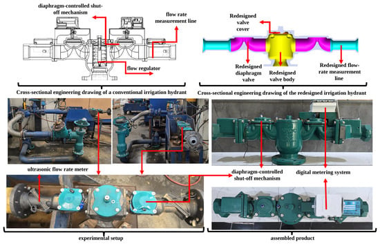
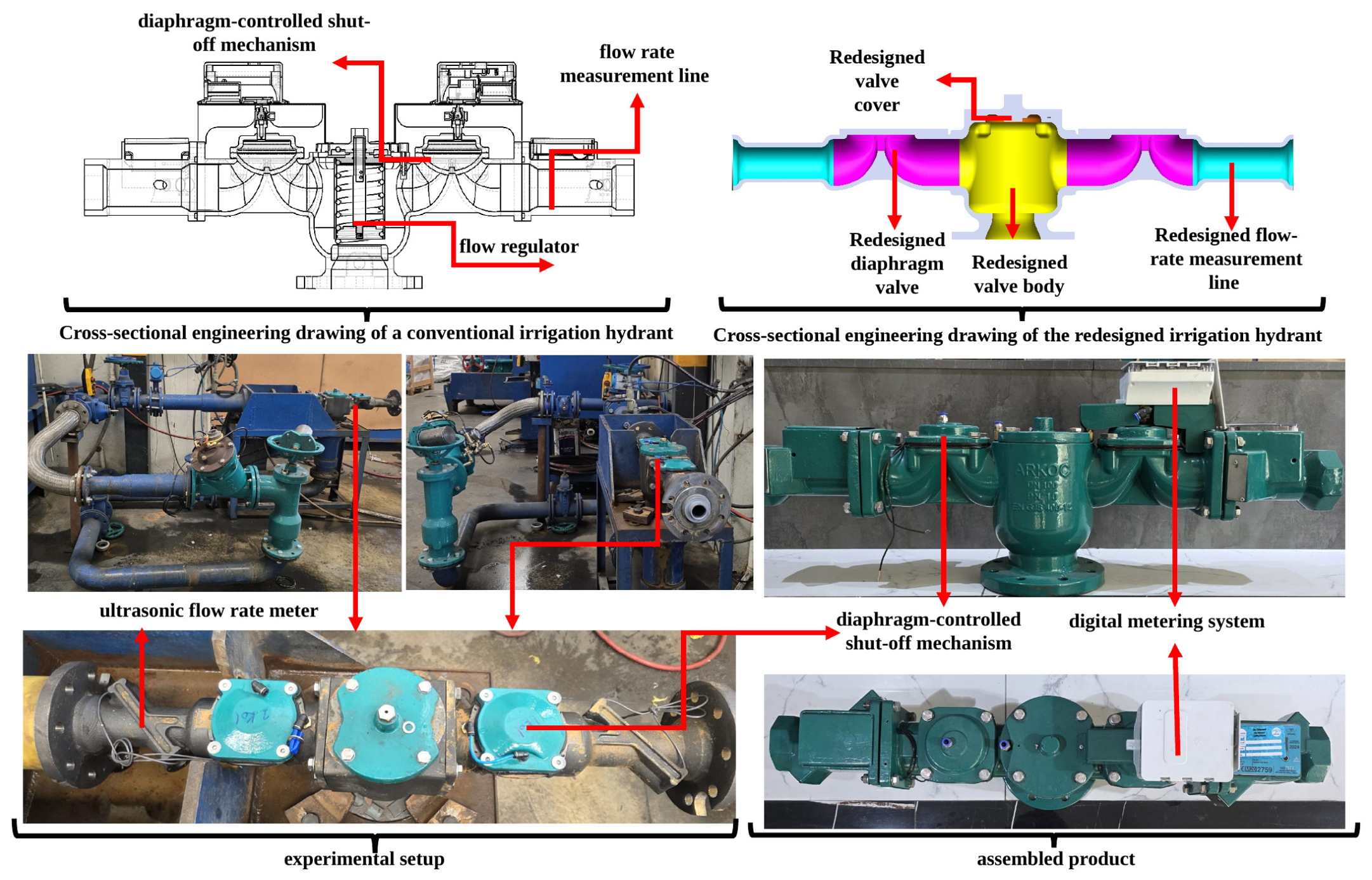
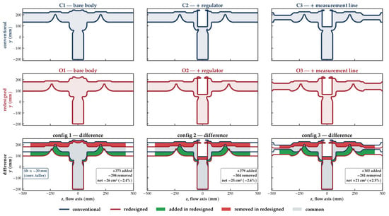
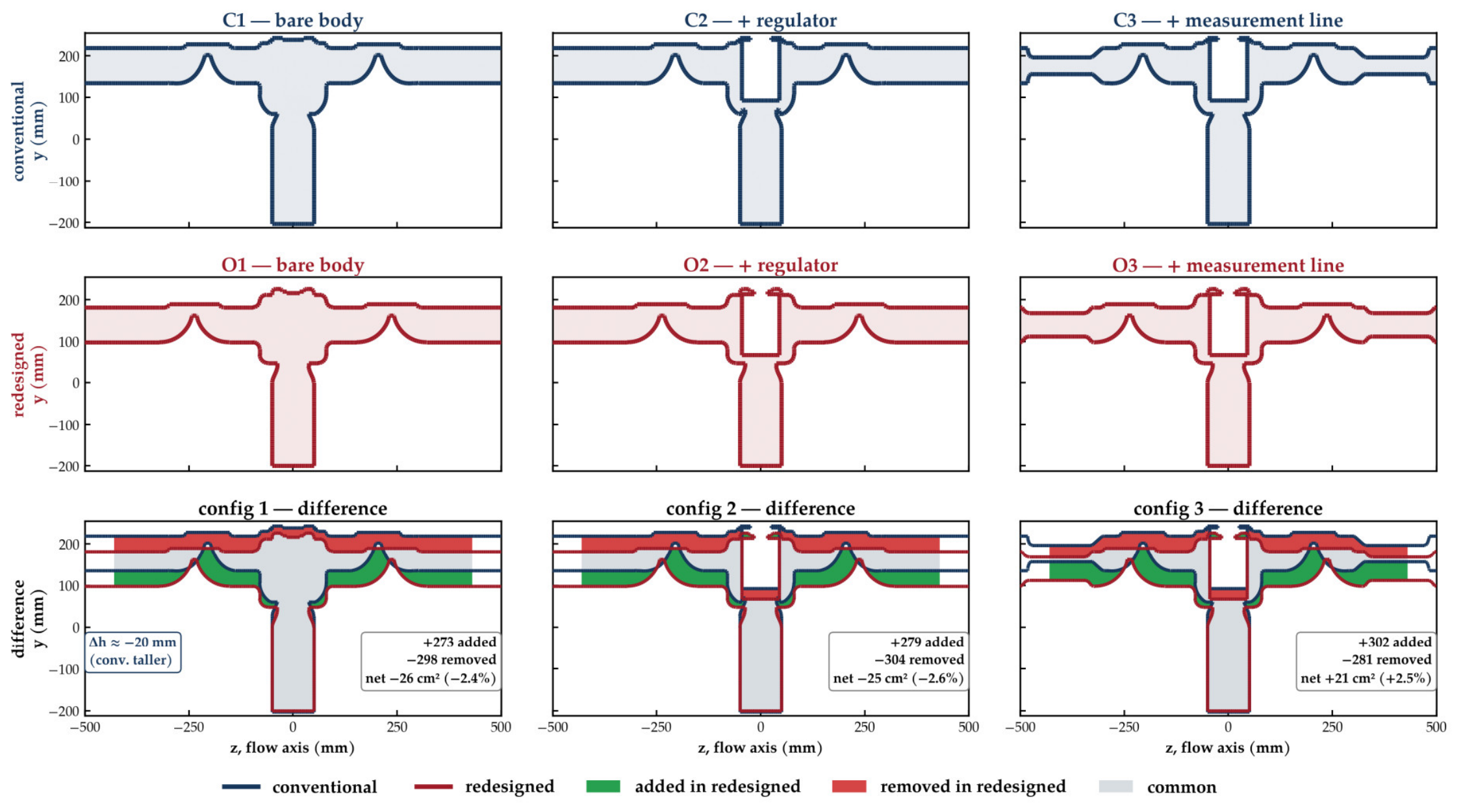
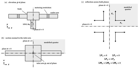
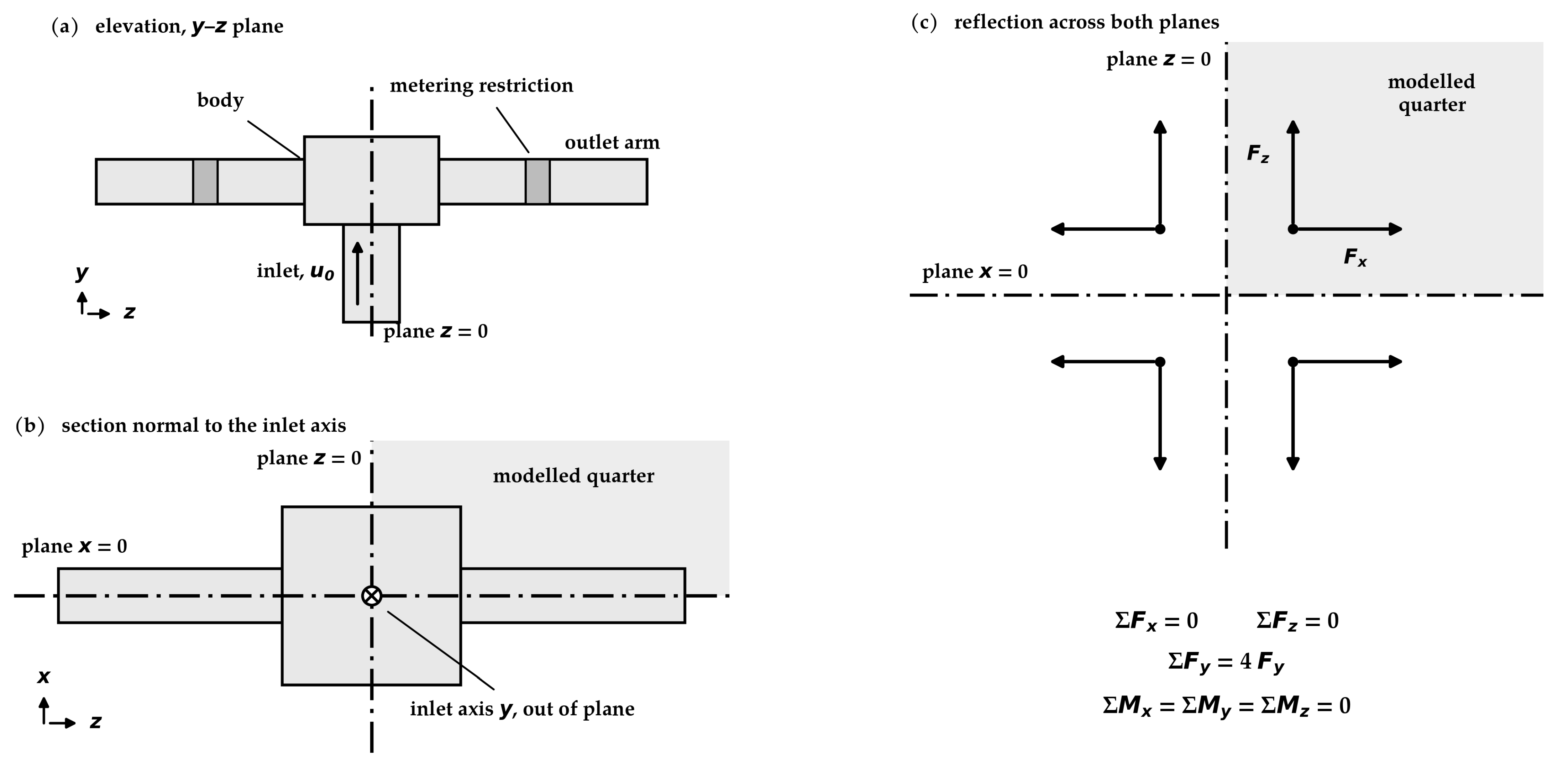
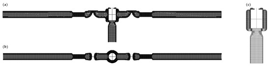
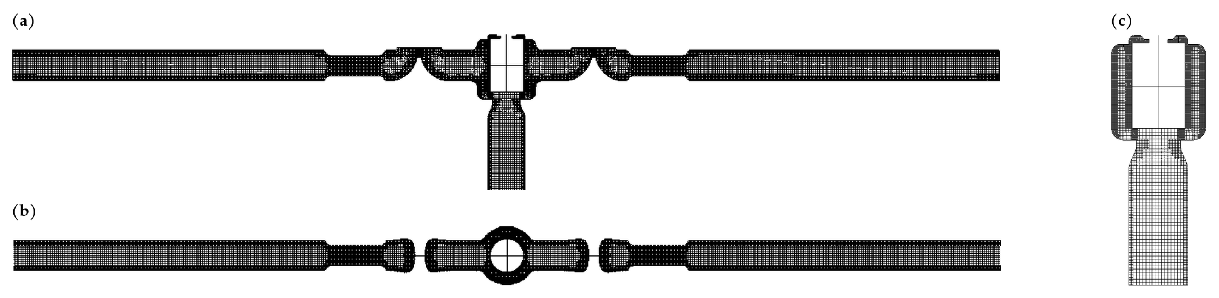
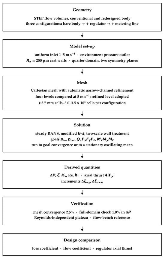
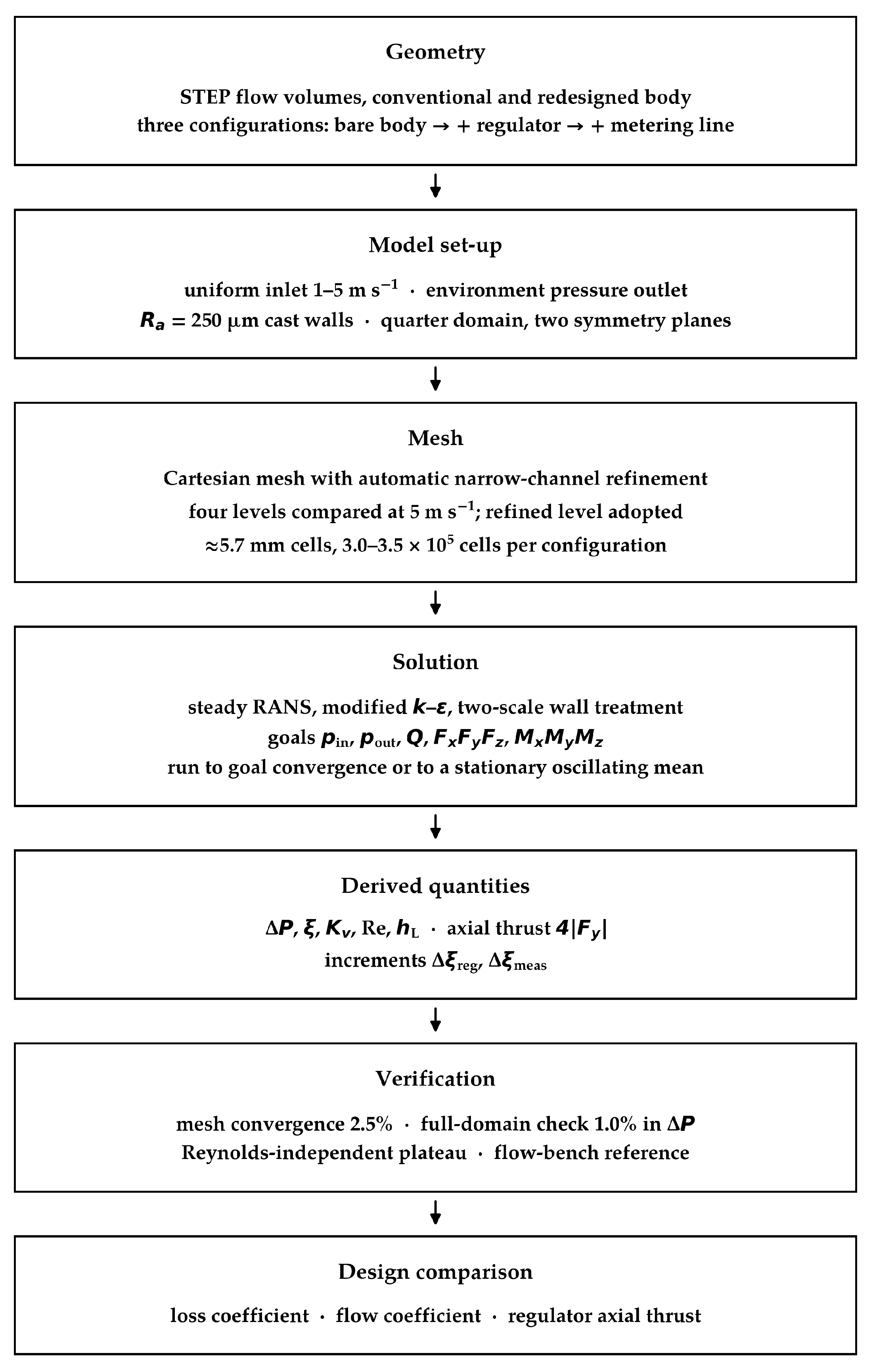
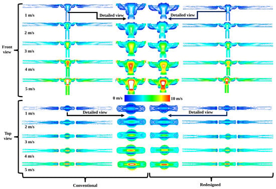
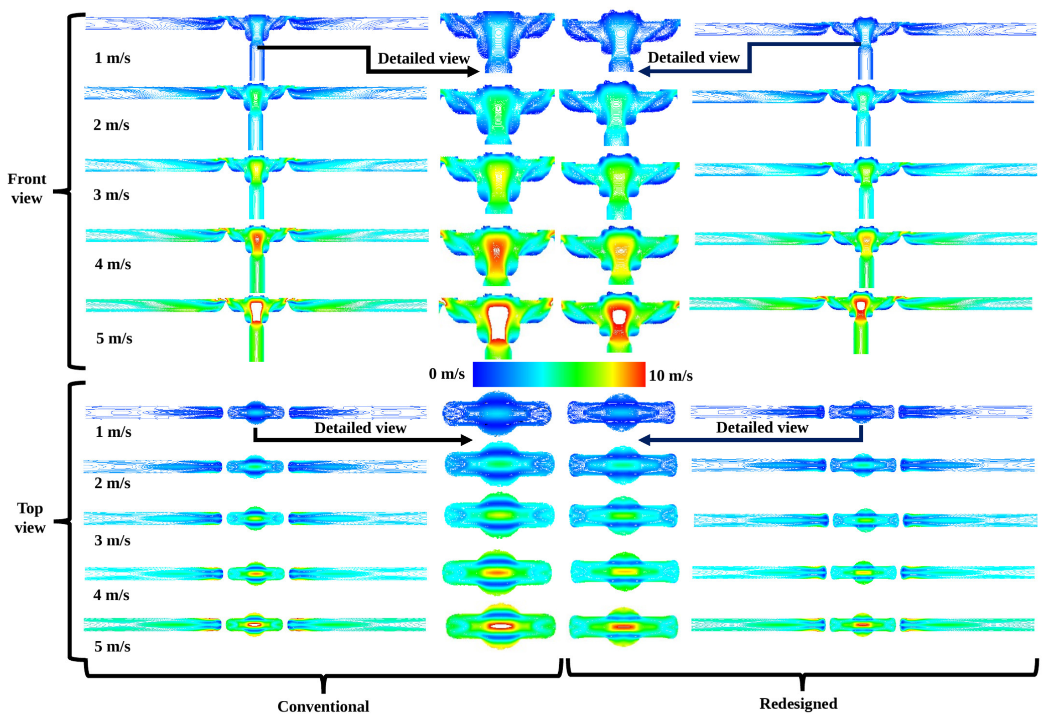
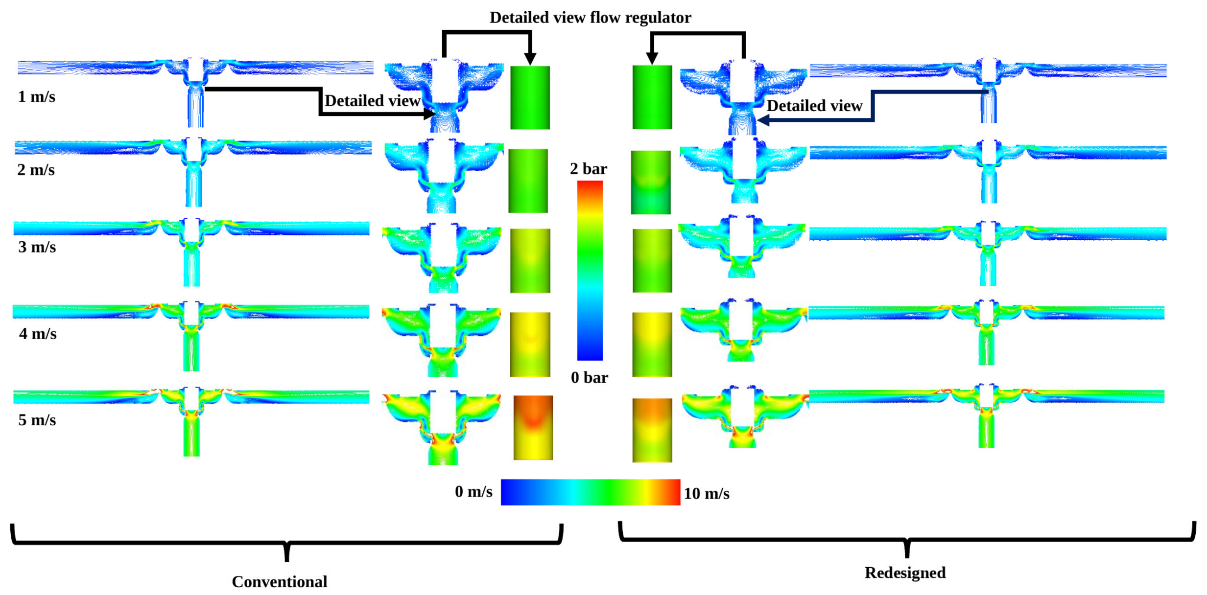
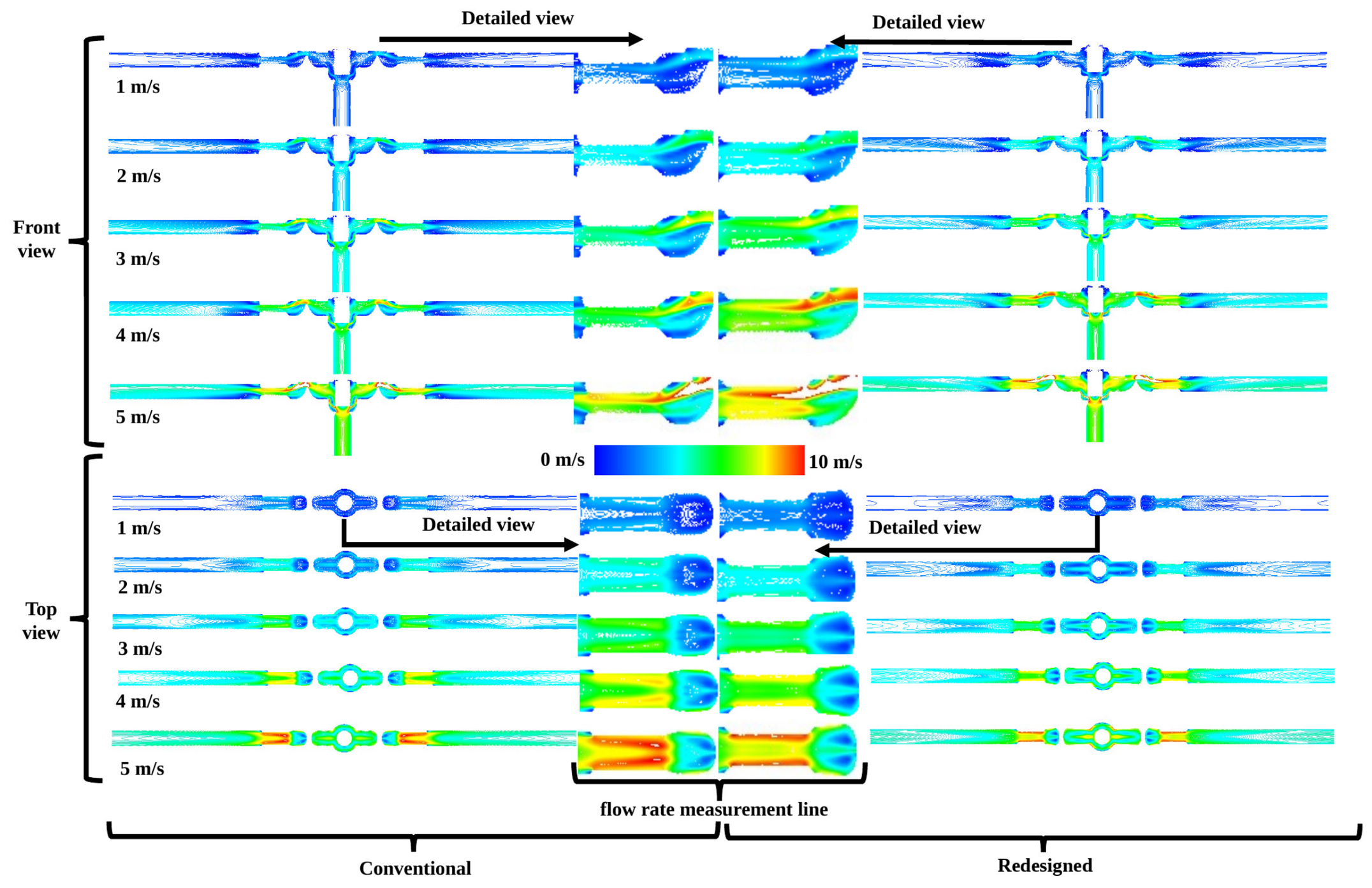
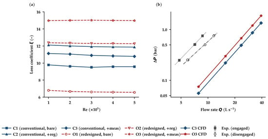
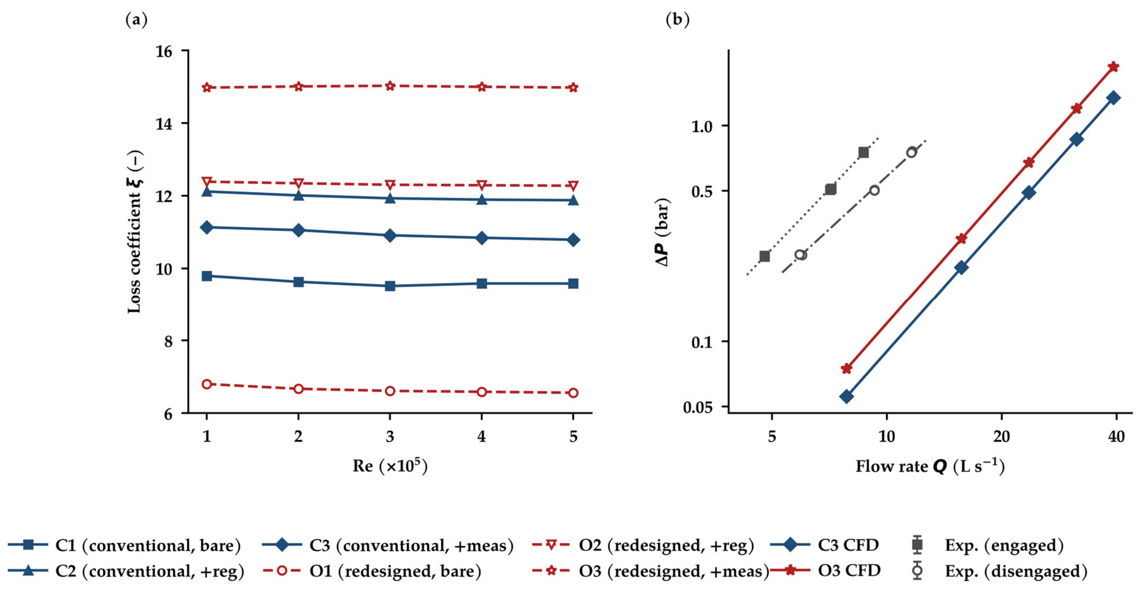
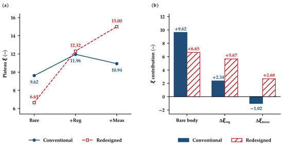
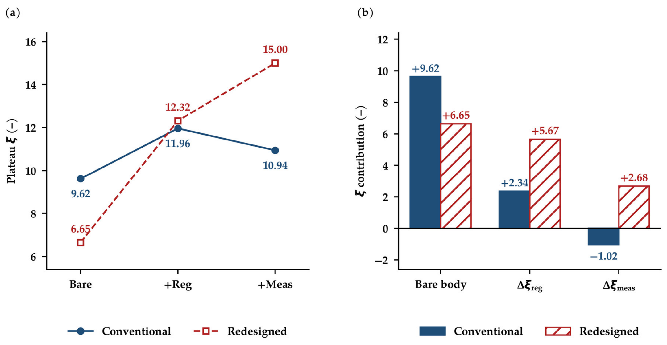
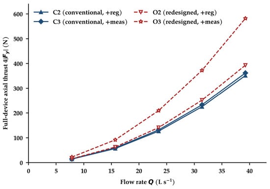
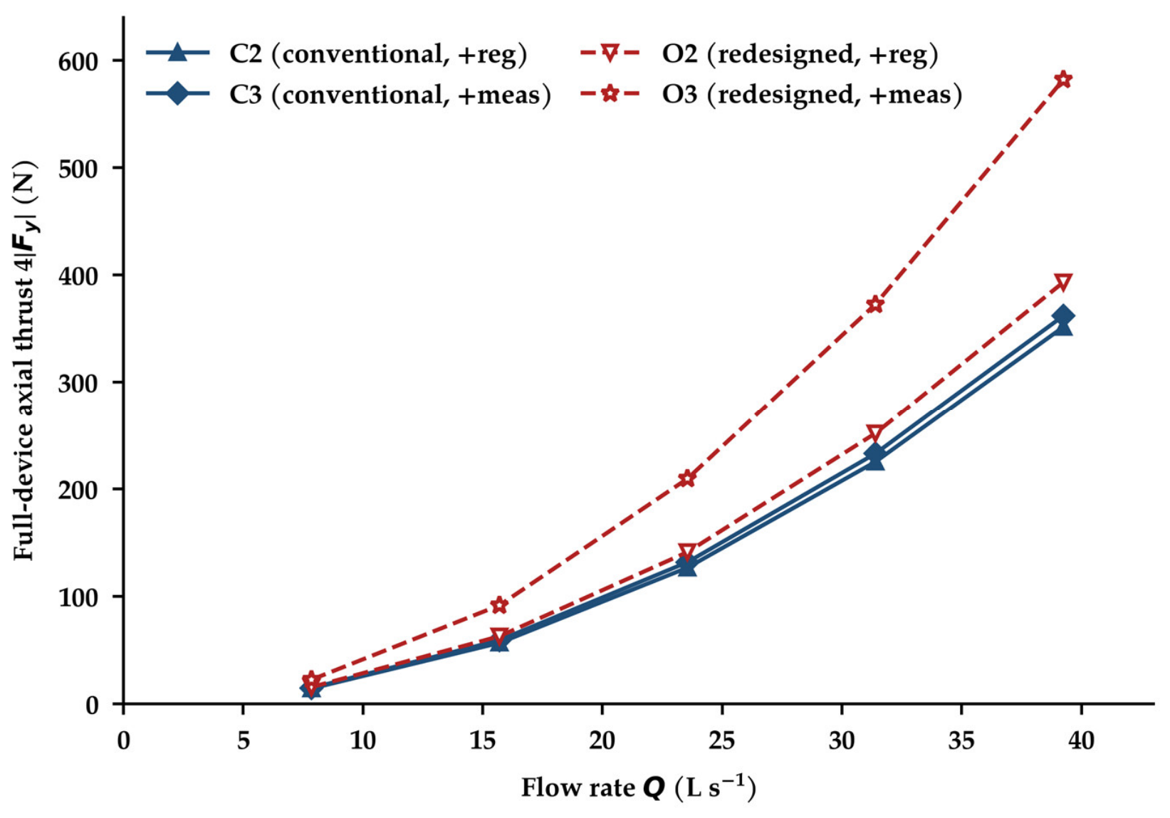
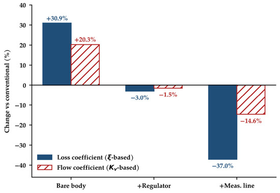
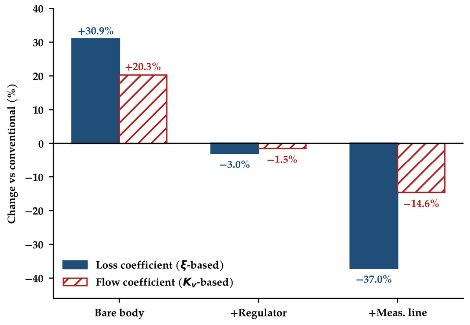
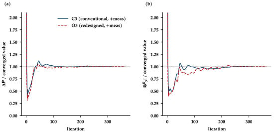
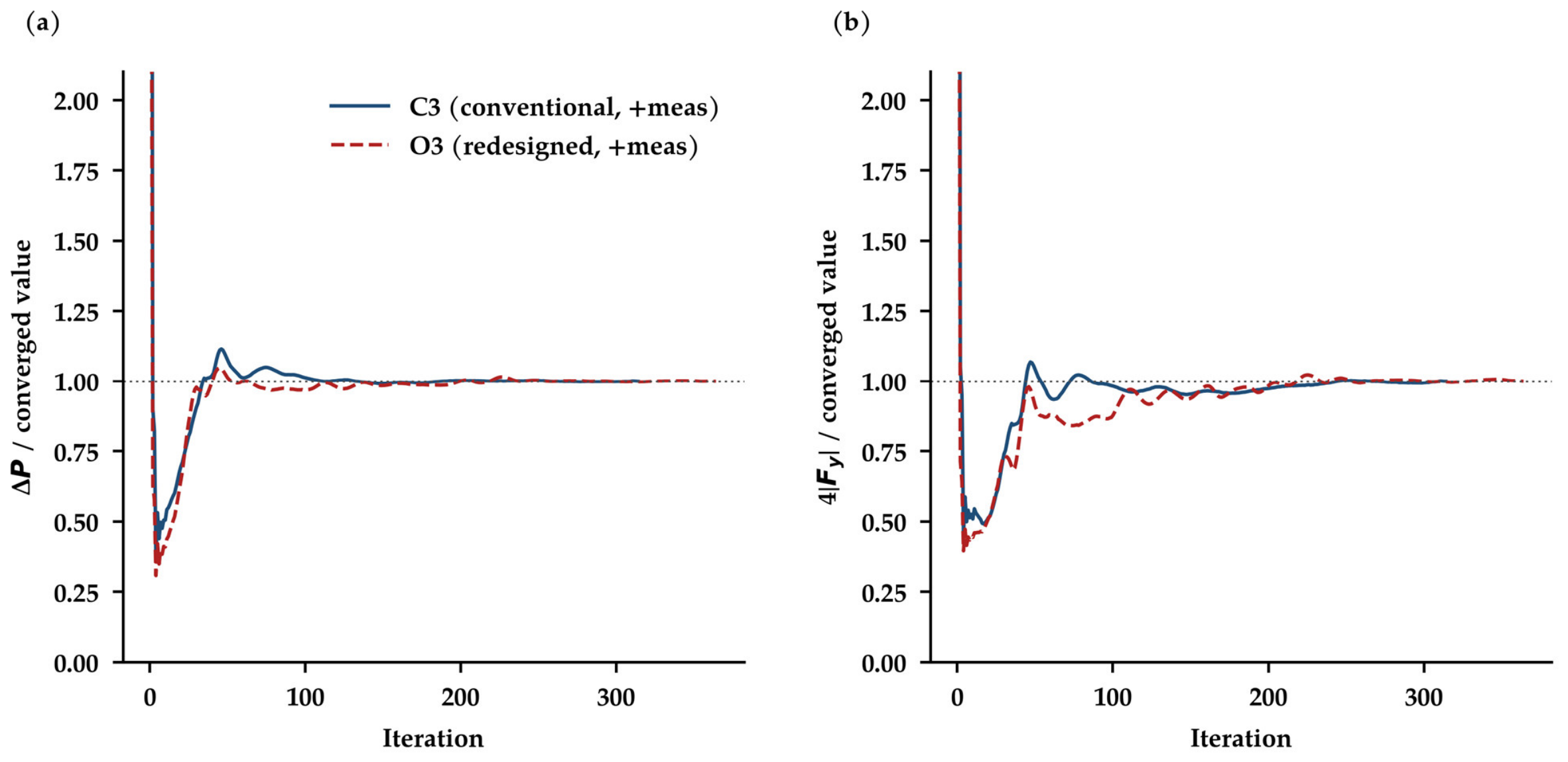
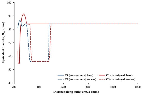
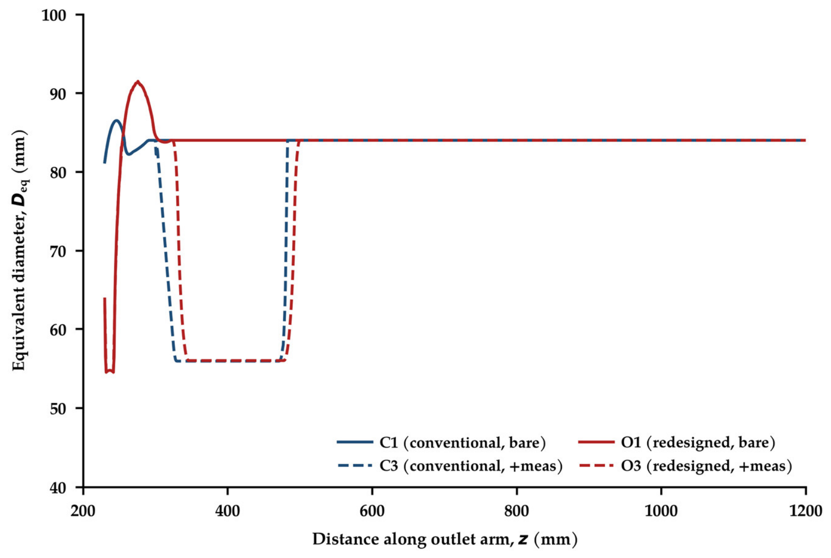
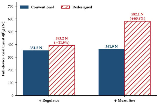
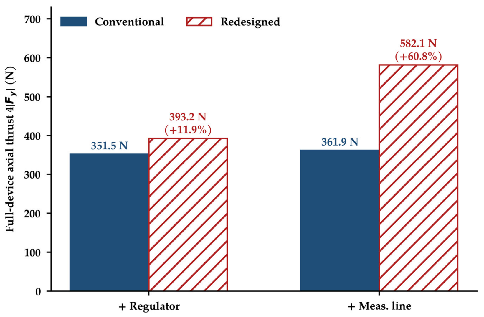

Disclaimer/Publisher’s Note: The statements, opinions and data contained in all publications are solely those of the individual author(s) and contributor(s) and not of MDPI and/or the editor(s). MDPI and/or the editor(s) disclaim responsibility for any injury to people or property resulting from any ideas, methods, instructions or products referred to in the content. |
© 2026 by the author. Licensee MDPI, Basel, Switzerland. This article is an open access article distributed under the terms and conditions of the Creative Commons Attribution (CC BY) license.