Multi-Regime Traffic Flow Modelling on Specific Urban Highway Infrastructures

Abstract

Vehicle arrival headways are among the fundamental microscopic traffic-flow characteristics and provide important information about vehicle interactions within traffic streams. This study investigates the statistical properties of vehicle arrival headways observed under different traffic operating conditions on urban motorway facilities. Traffic data were collected at six locations in the City of Zagreb, including open motorway sections, a tunnel, a bridge, and an underpass. Vehicle speeds and arrival headways were determined from digital video recordings using a frame-by-frame traffic observation methodology. The collected data were analysed using lognormal and shifted-lognormal distributions. The results showed that the observed headway distributions can be adequately represented by shifted-lognormal models. Relationships between the distribution parameters and selected traffic-flow characteristics were then investigated. Particular attention was devoted to average vehicle speed and the share of vehicles travelling in platoons. The analysis revealed the existence of two distinct traffic regimes. The first regime was characterised by higher average vehicle speeds and lower platoon shares, whereas the second regime was characterised by lower average speeds and higher platoon shares. Based on these observations, both a single-regime model and regime-specific models were developed for estimating the parameters of shifted-lognormal headway distributions. An internal assessment procedure demonstrated that the regime-specific models provide better agreement with observed headway distributions within their respective traffic conditions than a single model estimated from the complete dataset. The results indicate that accounting for differences in traffic operating conditions can improve the representation of vehicle arrival headways on urban motorway facilities.

1. Introduction

Traffic-flow characteristics observed on urban motorway facilities such as tunnels, bridges, and underpasses often differ from those observed on open motorway sections. These differences arise from variations in infrastructure geometry, traffic operating conditions, and driver behaviour, and are commonly reflected in vehicle speeds and headway distributions. Understanding such differences is important for traffic-flow analysis and for the development of models capable of describing vehicle arrival processes under different operating conditions. Time headway is one of the fundamental microscopic traffic-flow characteristics. In addition to describing vehicle arrival processes, time-headway distributions provide valuable information about traffic-stream behaviour and interactions between vehicles. Previous studies [1,2,3] have shown that different statistical distributions may be used to represent observed headway data under different traffic conditions. Consequently, identifying appropriate distribution models and understanding how their parameters vary with traffic conditions remains an important research topic. The present study is based on traffic measurements conducted in the City of Zagreb during spring 2025. Traffic data were collected at six observation locations representing different urban motorway environments, including open motorway sections, a tunnel, a bridge, and an underpass. Vehicle passage times and speeds were obtained from digital video recordings using a methodology previously developed and applied in [4]. The objective of the study is to investigate the statistical properties of vehicle arrival headways observed under different traffic operating conditions and to examine the relationship between the parameters of shifted-lognormal headway distributions and selected traffic-flow characteristics. Particular attention is given to the average vehicle speed and the share of vehicles travelling in platoons, which were found to be strongly associated with differences between the investigated traffic conditions. The analysis revealed the existence of two distinct groups of traffic conditions characterized by different combinations of average speed and platoon share. Consequently, both single-regime and regime-specific shifted-lognormal models are developed and evaluated. Their ability to represent observed headway distributions is assessed using independent groups of observations obtained from the six study locations. Although the results are based on a case study conducted in Zagreb, the proposed methodology can be applied to other urban motorway facilities where vehicle arrival headways are available and comparable traffic operating conditions exist. The remainder of the paper is organized as follows. Section 2 presents a review of related research. Section 3 describes the measurement methodology and data collection procedure. Section 4 presents the statistical analysis of time headways and the development of the proposed models. Section 5 evaluates the agreement between the proposed models and the observed data. Finally, Section 6 summarizes the principal findings and outlines directions for future research.

2. Literature Review

Traffic-flow theory deals with the movement of vehicles on road networks through the study and definition of fundamental traffic-flow variables. It also investigates traffic-flow characteristics under both ideal and real operating conditions, as well as the relationships between the fundamental traffic-flow parameters [5].

Traffic-flow theory emerged as a scientific discipline in the early 1930s. Since then, numerous empirical studies have investigated the relationships between vehicle speed, traffic density, and traffic flow under real-world conditions [4]. Greenshields [6] was among the first researchers to systematically investigate relationships between the fundamental traffic-flow variables, proposing a linear relationship between mean space speed and traffic density. Satisfactory agreement with empirical observations was achieved for low- and medium-density traffic flows. It was also observed that the linearity of the speed–density relationship increases as the observed traffic flow approaches ideal traffic conditions. Greenberg [7] studied traffic flow under the assumption that vehicle movement can be represented as a one-dimensional fluid and proposed a logarithmic relationship between mean space speed and traffic density. However, this model does not adequately represent low-density traffic conditions because the predicted mean speed tends towards infinity as density approaches zero, limiting its practical applicability. Underwood proposed an exponential speed–density relationship [8], whereas May proposed a bell-shaped relationship [9]. Other important contributions include the studies of Drew, Underwood, and Edie [5]. In addition to the aforementioned single-regime traffic-flow models, multi-regime models have also been developed, in which different relationships are applied to different ranges of traffic density [4]. The concept of multi-regime modelling is particularly relevant when traffic-flow characteristics exhibit distinct behavioural patterns under different operating conditions.

In addition to macroscopic traffic-flow models based on speed, flow, and density, numerous studies have investigated microscopic traffic characteristics through the analysis of vehicle headways. Headway distributions provide insight into vehicle interactions within traffic streams and have been widely applied in the modelling of traffic-flow operations and capacity-related phenomena.

The research presented in this paper focuses on the distribution of vehicle time headways, one of the fundamental variables in traffic-flow theory that has been extensively investigated over several decades. For example, Buckley [10] used a generalized semi-Poisson model to describe observed freeway headway distributions. Cowan [11] subsequently proposed four alternative models, namely M1 (Poisson process), M2 (shifted-exponential distribution), M3 (mixed exponential distribution), and M4 (mixed distribution with a general headway component), for modelling headway distributions under different traffic conditions. More recently, Zhang et al. [12] applied shifted-lognormal and double-displaced negative exponential distributions to model headway data collected on urban freeways. Ha et al. [13] compared several time-headway distribution models and evaluated their performance using traffic data collected on the French national road network. Li and Chen [14] conducted a comprehensive review of vehicle headway distribution models and highlighted the evolution of the assumptions underlying the most commonly used approaches.

Among the numerous distributions proposed in the literature, the lognormal and shifted-lognormal distributions have attracted considerable attention because of their ability to represent both free-flow and constrained traffic conditions. Their flexibility makes them particularly suitable for modelling heterogeneous traffic streams with varying proportions of platooned vehicles. Consequently, the present study adopts the shifted-lognormal distribution as the basis for modelling observed time-headway distributions under different traffic operating conditions.

3. Methodology of Traffic Flows Measurement

The methodology used for determining the basic traffic-flow characteristics at the vehicle level comprises three main steps:

• Selection of observation locations and observation periods;
• Collection of traffic data;
• Statistical analysis of the collected data and estimation of traffic-flow parameters.

The study investigates vehicle arrival headway distributions under different traffic operating conditions on characteristic and specific urban motorway infrastructures. Traffic data were collected at six observation locations (traffic directions):

• L1 and L2—straight sections of a four-lane suburban motorway (motorway A3—Zagreb Bypass), two traffic directions;
• L3—a two-lane urban tunnel (Aleja Bologne, Zagreb), one traffic direction;
• L4—a four-lane urban bridge (Ljubljanska avenija, Zagreb), one traffic direction;
• L5 and L6—a four-lane urban underpass (Zagrebačka avenija, Zagreb), two traffic directions.

The research was conducted at six locations in Zagreb selected to represent distinct urban motorway environments, including open motorway sections, a tunnel, a bridge, and an underpass. The objective was to examine whether differences in traffic operating conditions are associated with differences in the statistical properties of vehicle arrival headways. All traffic observations were conducted during April 2025 under stable weather conditions. No precipitation was recorded during any observation period, and the roadway surface remained dry throughout the measurements.

The principal characteristics of the observation locations, observation periods, traffic conditions, and traffic-flow characteristics are summarized in Table 1.

Table 1. Characteristics of observation locations and measurement conditions.

	L1	L2	L3	L4	L5	L6
Infrastructure type	Straight four-lane suburban motorway section		Urban two-lane tunnel	Urban two-lane bridge	Urban four-lane underpass
Number of lanes	4	4	2	2	4	4
Distance between observation lines (m)	42	42	27.8	25.6	25	25
Observation date	9 April	9 April	10 April	10 April	11 April	11 April
Observation period	10:15–11:22	11:32–12:27	13:23–15:06	15:15–15:39	13:06–13:38	13:47–14:24
Observation duration (min)	67	55	103	24	32	37
Vehicles observed	478	475	590	483	482	465
Traffic flow rate (veh/h)	428.1	518.2	343.7	1207.5	903.8	754.1
Mean vehicle speed (km/h)	54.7	56.0	51.6	36.0	38.8	36.2
Share of vehicles in platoons (%)	60.0	77.8	78.6	97.9	94.4	92.7

To provide additional insight into the observed traffic conditions, the composition of traffic flows at the six observation locations is summarized in Table 2. The table presents the proportions of passenger cars, motorcycles, light goods vehicles, heavy goods vehicles, and buses recorded at each location.

Table 2. Percentage share of vehicle categories at the observation locations.

	L1	L2	L3	L4	L5	L6
Cars	71.0	71.4	83.5	83.7	80.5	77.5
Motorcycles	0.0	0.2	0.8	0.8	0.4	0.4
Light goods vehicles (LGVs)	5.4	7.8	7.1	5.8	9.6	8.4
Heavy goods vehicles (HGVs)	22.4	20.0	6.3	9.5	9.4	13.5
Buses	1.2	0.6	2.3	0.2	0.0	0.2

Although vehicle composition was not explicitly included in the subsequent regression models, it is reported here to facilitate comparison between the investigated locations and to provide additional context for the observed differences in traffic-flow characteristics.

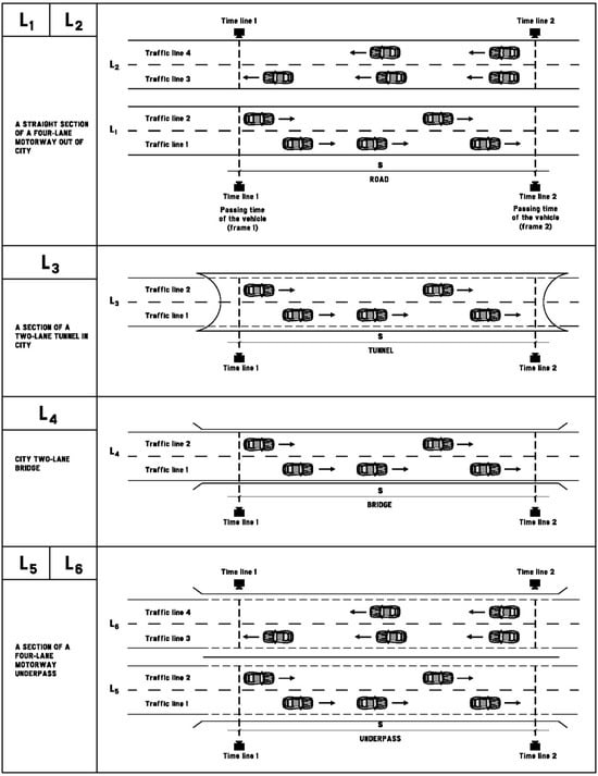
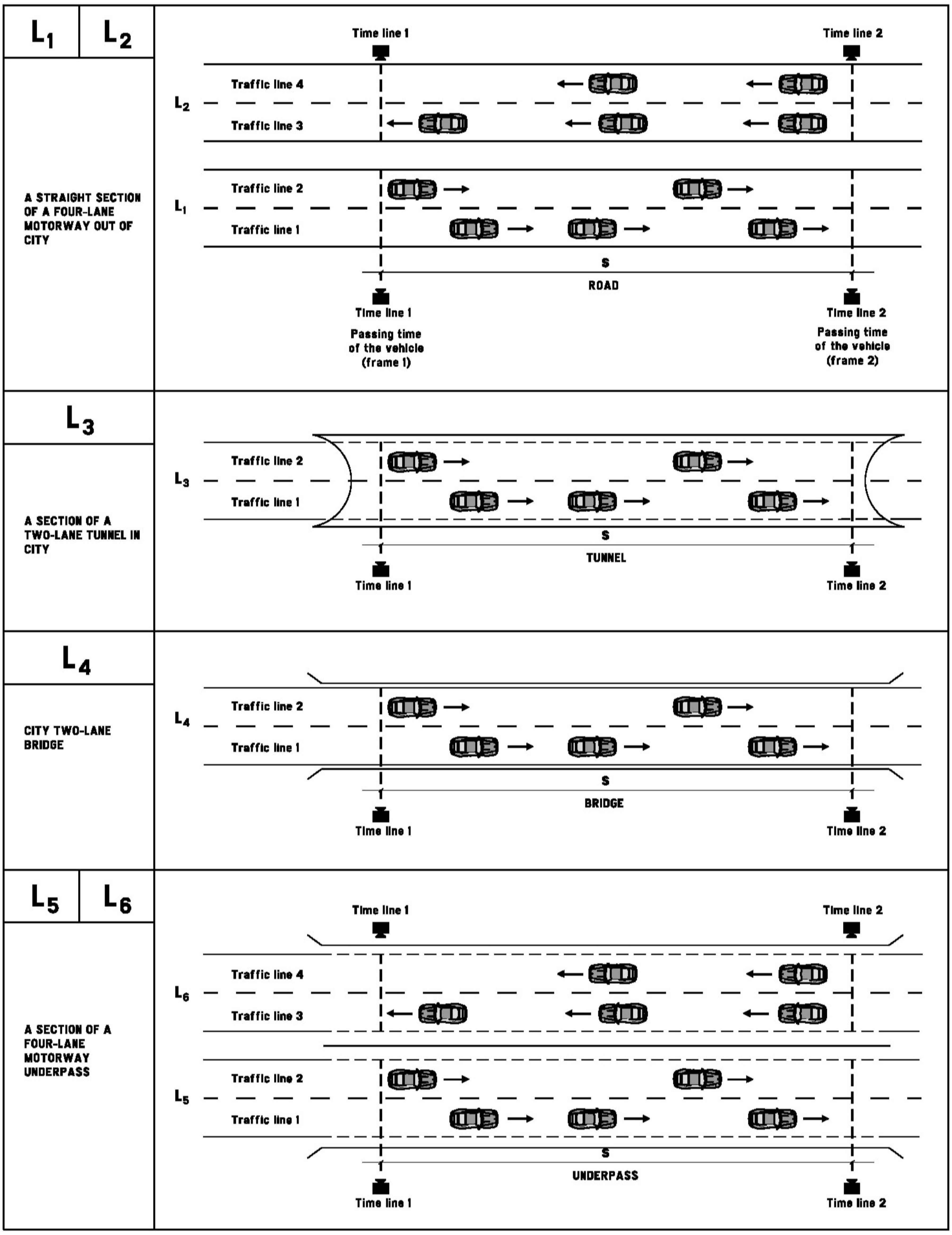
To collect vehicle-speed and time-headway data, an adapted traffic observation methodology previously applied in [4] was used. For each location, an observation section was defined by establishing two observation lines and measuring the distance between them. Traffic movements were then recorded using digital video cameras (Figure 1). Digital video cameras capable of recording in MTS and MP4 formats at a frame rate of 50 fps (frames per second) were used in the study. Higher frame rates provide more precise estimates of vehicle passage times and vehicle speeds.

Figure 1. Scheme of the observation section showing the two observation lines used for determining vehicle passage times and speeds. The direction of the arrows indicates the direction of vehicle movement.

In the next step, the collected traffic data were transformed into a format suitable for statistical analysis. Video recordings were analysed frame-by-frame and, for each vehicle, the frame number corresponding to the passage of the first and the second observation line was recorded. By definition, the frame number corresponding to a vehicle crossing an observation line was taken as the first frame in which the front axle of the vehicle reached the observation line. The database contains the frame numbers corresponding to vehicle passages across the first and second observation lines, together with the vehicle category (passenger car, motorcycle, light goods vehicle, heavy goods vehicle, or bus). These data provide information on the traffic-flow composition at each observation location. The collected data make it possible to determine, for each observed vehicle, its mean speed, the time headway, and the corresponding estimated space headway.

Let $A_1,A_2,\dots ,A_N$ denote all vehicles that passed through the selected road section during the observation period T. Vehicles were ordered according to their observed passage times regardless of lane position. Consequently, the analysed sequence represents the aggregate arrival process at the observation cross-section. Furthermore, let $F_{L1}^i$ and $F_{L2}^i$ denote the frame number in which vehicle $A_i$ crosses the first and the second observation line, respectively. Then the travel time of vehicle $A_i$ along the observation section, $\Delta t_i$, is defined by:

$${\Delta t}_i={\displaystyle \frac{F_{L2}^i-F_{L1}^i}{\mathit{fps}}}\left[s\right],$$

where fps is the recording speed of the video camera.

Let $v_i$ denote the mean speed of vehicle $A_i$ on the selected road section. Then

$$v_i={\displaystyle \frac{s}{\Delta t_i}}={\displaystyle \frac{s·\mathit{fps}}{F_{L2}^i-F_{L1}^i}}[m/s],$$

where s is the length of the observed section (distance between the first and the second line of observation).

The time headway represents the time interval between two consecutive vehicle arrivals in the aggregated traffic stream at the observation cross-section. Since two observation lines were used, the time headway between vehicle $A_i$ and the preceding vehicle $A_{i-1}$ was calculated as the arithmetic mean of the headways measured at the first and the second observation line. Formally, let $t_{h1}^i$ and $t_{h2}^i$ denote the time headway of vehicles $A_i$ and $A_{i-1}$ on the first and the second line of observation:

$$t_{h1}^i={\displaystyle \frac{F_{L1}^i-F_{L1}^{i-1}}{\mathit{fps}}}\left[s\right];t_{h2}^i={\displaystyle \frac{F_{L2}^i-F_{L2}^{i-1}}{\mathit{fps}}}\left[s\right].$$

Then, the time headway of vehicles $A_i$ and $A_{i-1}$ on the selected road section, $t_h^i$, is defined as

$$t_h^i={\displaystyle \frac{1}{2}}\left(t_{h1}^i+t_{h2}^i\right)={\displaystyle \frac{1}{2}}·\left({\displaystyle \frac{F_{L1}^i-F_{L1}^{i-1}}{\mathit{fps}}}+{\displaystyle \frac{F_{L2}^i-F_{L2}^{i-1}}{\mathit{fps}}}\right)\left[s\right].$$

An estimated space headway was calculated as the product of the aggregated time headway and the mean speed of vehicle $A_i$. This quantity should be interpreted as a derived measure of vehicle spacing and not as a directly observed instantaneous distance between two vehicles. Therefore, for vehicle $A_i$, the estimated space headways on the first and the second observation line, $s_{h1}^i$ and $s_{h2}^i$, are defined as

$$s_{h1}^i=v_i·t_{h1}^i\left[m\right];s_{h2}^i=v_i·t_{h2}^i\left[m\right].$$

The estimated space headway on the selected road section for vehicle $A_i$ is defined as the arithmetic mean of the estimated space headways calculated at the first and second observation line:

$$s_h^i={\displaystyle \frac{1}{2}}\left(s_{h1}^i+s_{h2}^i\right)={\displaystyle \frac{1}{2}}·\left(v_i·t_{h1}^i+v_i·t_{h2}^i\right)={\displaystyle \frac{v_i}{2}}\left(t_{h1}^i+t_{h2}^i\right)=v_i·t_h^i\left[m\right].$$

Because vehicles from all lanes were merged into a single chronological sequence, the calculated time headways describe aggregate inter-arrival characteristics at the observation cross-section. Consequently, the estimated space headways should not be interpreted as lane-specific vehicle spacings arising from microscopic car-following behaviour. Their purpose in this study is to characterize the statistical properties of the aggregated traffic stream under different traffic operating conditions.

In this study, a platoon is defined as a sequence of vehicles separated by time headways shorter than 5 s. Accordingly, a vehicle is considered to be travelling in a platoon if its time headway with respect to the preceding vehicle is less than 5 s. The threshold value of 5 s was adopted from the methodology developed in [4] and was retained to ensure methodological consistency with previous investigations conducted on comparable urban motorway infrastructures.

The selected threshold was used to distinguish vehicles travelling as part of a constrained traffic stream from vehicles travelling under relatively free-flow conditions. It should be noted that no universally accepted time-headway threshold exists for the identification of platoons [15,16,17,18,19,20,21,22]. Reported threshold values vary across studies depending on roadway type, traffic conditions, and research objectives. Consequently, the choice of a platoon threshold inevitably involves a degree of engineering judgement. The share of vehicles travelling in platoons, denoted by P, was calculated as

$$P={\displaystyle \frac{N_P}{N}}·100[\%],$$

where $N_P$ denotes the number of vehicles classified as belonging to platoons and N denotes the total number of observed vehicles. Because platoons are identified from aggregate vehicle arrivals across all lanes, the resulting platoon share P reflects the frequency of short inter-arrival times within the aggregated traffic stream. Consequently, it represents an operational traffic-flow indicator rather than a direct measure of lane-specific car-following behaviour.

Table 3 presents an illustrative excerpt from the processed vehicle database. The example demonstrates the determination of vehicle travel times, speeds, time headways, and estimated space headways from recorded frame numbers. In this example, vehicles 8 and 9 form one platoon, whereas vehicles 11, 12, and 13 form another platoon.

Table 3. Example of the processed vehicle database used for traffic-flow analysis.

1	2	3	4	5	6	7	8	9
Vehicle Number ($\mathit{i}$)	Type of Vehicle	Number of Frames ${\mathit{F}}_{\mathit{L}\mathit{1}}^{\mathit{i}}$ and ${\mathit{F}}_{\mathit{L}\mathit{2}}^{\mathit{i}}$		Time Interval of Passing the Section $\Delta {\mathit{t}}_{\mathit{i}}$	Mean Vehicle Speed ${\mathit{v}}_{\mathit{i}}$	Vehicle Time Headway ${\mathit{t}}_{\mathit{h}}^{\mathit{i}}$	Estimated Space Headway ${\mathit{s}}_{\mathit{h}}^{\mathit{i}}$	Platoon ID
7	A	1437	1589	152.0	13.82	5.46	75.43	0
8	A	2094	2219	125.0	16.80	12.87	216.22	1
9	A	2151	2303	152.0	13.82	1.41	19.48	1
10	A	2990	3122	132.0	15.91	16.58	263.77	0
11	A	3416	3532	116.0	18.10	8.36	151.34	2
12	A	3532	3624	92.0	22.83	2.08	47.48	2
13	A	3547	3670	123.0	17.07	0.61	10.41	2
14	A	4015	4111	96.0	21.88	9.09	198.84	0

4. Statistical Analysis of Time Headway

Time headways are important not only in the analysis of individual vehicle movement but also in the characterization of traffic-flow operations. Time-headway distributions provide insight into the microscopic characteristics of traffic streams. The literature [1,2,3] states that a low-flow time-headway distribution matches the exponential distribution, whereas for high flow, when the distance between vehicles is smaller, a normal distribution is used, but for the modelling of the time headway distribution, other distributions may also be used, such as lognormal [3,23] and shifted-lognormal. By definition, a positive random variable X with parameters $\mu$ and ${\sigma }^2$, in denotation $\mathrm{\Lambda }(\mu ,{\sigma }^2)$, is said to be lognormally distributed if random variable $Y=\ln X$ is normally distributed with mean $\mu$ and variance ${\sigma }^2$ [24]. In addition, a random variable X with parameters $\tau$, $\mu$ and ${\sigma }^2$ is said to be a shifted-lognormal random variable if the random variable $Y=X-\tau$ is lognormal, $Y=\mathrm{\Lambda }(\mu ,{\sigma }^2)$. Thus the lognormal distribution is a special case of the shifted-lognormal distribution for which $\tau =0$. The shifted-lognormal distribution X with parameters $\tau$, $\mu$ and ${\sigma }^2$ is denoted by $\mathrm{\Lambda }(\tau ,\mu ,{\sigma }^2)$.

In order to determine whether the observed data $x_1,\dots ,x_n$ match some statistical distribution, it is necessary to find the parameters of distribution and to perform a statistical test that will study how well the empirical data are represented by the given distribution. The Maximum Likelihood Estimation (MLE) method was used to estimate the distribution parameters, and other methods can be used, such as minimum distance estimation, maximum spacing estimation, method of moments, etc. Basically, in the MLE method, the distribution parameters are determined so that the probability of occurrence of empirical data is the largest possible. Such an approach leads to solving a system of non-linear equations, but for many important distributions there are closed formulas for calculating their parameters from empirical data. The formulas for estimating the parameters of normal, exponential and lognormal distributions [25] are presented in Table 4.

Table 4. The maximum likelihood estimators of the parameters of normal, exponential, and lognormal distributions from a sample of observations $x_1,\dots ,x_n$. The numbers $\widehat{\mu }$, ${\widehat{\sigma }}^2$ and $\widehat{\lambda }$ are estimated values of corresponding parameters.

Normal Distribution $\mathit{N}(\mathit{\mu },{\mathit{\sigma }}^2)$	Exponential Distribution $\mathit{E}\left(\mathit{\lambda }\right)$	Lognormal Distribution $\mathbf{\Lambda }(\mathit{\mu },{\mathit{\sigma }}^2)$
${\displaystyle \widehat{\mu }=\frac{1}{n}(x_1+\cdots +x_n)}$	${\displaystyle \widehat{\lambda }=\frac{n}{x_1+\cdots +x_n}}$	${\displaystyle \widehat{\mu }=\frac{1}{n}(\ln x_1+\cdots +\ln x_n)}$
${\displaystyle {\widehat{\sigma }}^2=\frac{1}{n}{\displaystyle \sum _{i=1}^n}{(x_i-\widehat{\mu })}^2}$		${\displaystyle {\widehat{\sigma }}^2=\frac{1}{n}{\displaystyle \sum _{i=1}^n}{(\ln x_i-\widehat{\mu })}^2}$

In case of a shifted-lognormal distribution, the problem lies in the determination of the value of the shift $\tau$. For a given $\tau$ the determination of parameters $\mu$ and ${\sigma }^2$ is the same as for the lognormal distribution, but on data $x_1-\tau ,\dots ,x_n-\tau$.

Table 5 shows the results of the Kolmogorov–Smirnov and Anderson–Darling tests for matching of empirical data with the lognormal, normal and exponential distributions. The distribution parameters are calculated by the MLE method (Table 4) for all groups of data. The p-value of the test is shown for all cases. The symbol **** indicates that the test shows that the probability of data coming from a selected distribution is negligibly small (p-value less than ${10}^{-5}$).

Table 5. p-values for goodness-of-fit test.

	Lognormal Distribution		Normal Distribution		Exponential Distribution
Location	KS Test	AD Test	KS Test	AD Test	KS Test	AD Test
L1	0.917	0.546	****	****	****	****
L2	0.905	0.877	****	****	0.132	0.017
L3	0.0162	0.0149	****	****	****	****
L4	0.136	0.109	0.0007	0.00005	****	****
L5	0.219	0.146	****	****	****	****
L6	0.119	0.0931	****	****	****	****

****—p-value is smaller than 0.00001.

The reported p-values were obtained using conventional goodness-of-fit tests after estimating the distribution parameters from the same observations. Consequently, the p-values should be interpreted as descriptive indicators of agreement rather than exact significance levels.

As can be seen from Table 5, both the Kolmogorov–Smirnov and Anderson–Darling tests indicate good agreement between the observed data and the lognormal distribution at the 0.01 significance level for all investigated locations. The lowest p-value was obtained for data from location L3. Tests in which the data behave in accordance with the normal distribution have in all cases shown negligible significance. According to both tests, the exponential distribution cannot be rejected for the data obtained at location L2; however, this is not the case for the remaining locations.

The next step was to determine the relationship between the parameters of the shifted-lognormal distribution describing the observed time-headway data and the available traffic-flow characteristics. To obtain multiple independent observations from each location, the recorded vehicle sequences were divided into groups. The necessary traffic-flow and distribution parameters were then calculated for each group and used in subsequent analyses. For each location, the sequence of observed vehicles was divided into $K=4$ non-overlapping groups of approximately equal size, resulting in a total of 24 independent groups for subsequent analysis.

Let $A_1,A_2,\dots ,A_N$ denote all vehicles that passed a selected road section. These vehicles are arranged into K groups $C_1,\dots ,C_K$. Let $S\left(i\right)$ denote the number of vehicles in group $C_i$. Group $C_1$ consists of the first $S\left(1\right)$ vehicles $(A_1,\dots ,A_{S\left(1\right)})$, group $C_2$ consists of the following $S\left(2\right)$ vehicles $(A_{S\left(1\right)+1},\dots ,A_{S\left(1\right)+S\left(2\right)})$, etc. Value $S\left(i\right)$ is defined by

$$S\left(i\right)=\left\{\begin{array}{cc}M+1,& i\le L;\\ M,& i>L\end{array}\right.,$$

where parameters M and L are defined so that $N=K·M+L$, i.e., M is the result of integer division of N by K, whereas L is the remainder of the division of N by K.

In this way, a total of 24 independent groups were generated. For each group $C_i$, the following quantities were calculated:

• $V_i$—mean vehicle speed within group $C_i$;
• $P_i$—share of vehicles travelling in platoons within group $C_i$;
• ${\widehat{\mu }}_i$, ${\widehat{\sigma }}_i^2$—estimates of the parameters of the lognormal distribution (shift equal to zero) for group $C_i$, determined so as to minimize the value of the Kolmogorov–Smirnov statistic for the data in the group;
• ${\widehat{\mu }}_i^S$, ${\widehat{\sigma }}_i^{2,S}$ and ${\widehat{\tau }}_i^S$—estimates of the parameters of the shifted-lognormal distribution for group $C_i$, determined so as to minimize the value of the Kolmogorov–Smirnov statistic for the data in the group.

The procedure used to determine the parameters of the shifted-lognormal distribution that minimize the value of the Kolmogorov–Smirnov statistic for a given group of vehicles is described in Algorithm 1. Starting from the maximum-likelihood estimates of the corresponding lognormal distribution, the algorithm iteratively explores neighbouring values of the parameters $\mu$ and ${\sigma }^2$. For each candidate pair $(\mu ,{\sigma }^2)$, the shift parameter $\tau$ is varied over the interval $0\le \tau <{\tau }_{\max }$, where ${\tau }_{\max }$ denotes the smallest observed time headway within the analysed group. In the implementation used in this study, the search procedure was performed with $n_S=50$, $\Delta \mu =0.25/n_S$, $\Delta {\sigma }^2=0.25/n_S$, and $\Delta \tau ={\tau }_{\max }/50$. The procedure terminates after all candidate parameter combinations generated around the initial maximum-likelihood estimates have been evaluated.

Algorithm 1 Determination of shifted-lognormal distribution parameters minimizing the Kolmogorov–Smirnov statistic.
Parameters: $n_S$—number of steps in the given direction, $\Delta \mu$, $\Delta {\sigma }^2$, $\Delta \tau$—step-length in the given direction. Let $D(\mu ,{\sigma }^2,\tau )$ denote the value of the Kolmogorov–Smirnov statistic measuring the distance between the empirical distribution function of sample X and the shifted-lognormal distribution $L\sim \mathrm{\Lambda }(\mu ,{\sigma }^2,\tau )$.
S0:	Start
S1:	Let ${\tau }_{\max }=\min X=\min \left\{x_1,x_2,\dots ,x_n\right\}$.
S2:	Calculate $\widehat{\mu }$, ${\widehat{\sigma }}^2$, the maximum-likelihood estimates of the lognormal-distribution parameters obtained from sample X.
S3:	Let ${\mu }_T=\widehat{\mu }$, ${\sigma }_T^2={\widehat{\sigma }}^2$
S4:	For each $i,j\in \{-n_S,\dots ,n_S\}$
S5:	Let ${\mu }_{ij}={\mu }_T+i·\Delta \mu$, ${\sigma }_{ij}^2={{\sigma }_T}^2+j·\Delta {\sigma }^2$.
S6:	$k=0$: ${\tau }_0=0$.
S7:	Do While ${\tau }_k<{\tau }_{\max }$
S8:	Let $D_{ij}^{{\tau }_k}=D({\mu }_{ij},{\sigma }_{ij}^2,{\tau }_k)$.
S9:	$k=k+1$: ${\tau }_k=k·\Delta \tau$.
S10:	Loop
S11:	Let $D_{ij}^{\ast }={\min }_k{D}_{ij}^{{\tau }_k}$ and ${\tau }_{ij}$ is the value determined such that $D({\mu }_{ij},{\sigma }_{ij}^2,{\tau }_{ij})$ is equal to $D_{ij}^{\ast }$.
S12:	Next
S13:	Let $D^{\ast }={\min }_{ij}{D}_{ij}^{\ast }$, and let $i^{\ast }$ and $j^{\ast }$ be determined such that $D_{i^{\ast }{j}^{\ast }}^{\ast }=D^{\ast }$. Then ${\mu }_m={\mu }_{i^{\ast }{j}^{\ast }}$, ${\sigma }_m^2={\sigma }_{i^{\ast }{j}^{\ast }}^2$, and ${\tau }_m={\tau }_{i^{\ast }{j}^{\ast }}$.
S14:	If $(i^{\ast }=-n_S)$ Or $(i^{\ast }=n_S)$ Or $(j^{\ast }=-n_S)$ Or $(j^{\ast }=n_S)$ Then
S15:	If $(i^{\ast }=-n_S)$ Then ${\mu }_T={\mu }_m-n_S\Delta \mu$ Else If $(i^{\ast }=n_S)$ Then ${\mu }_T={\mu }_m+n_S\Delta \mu$
S16:	If $(j^{\ast }=-n_S)$ Then ${\sigma }_T^2={\sigma }_m^2-n_S\Delta {\sigma }^2$ Else If $(j^{\ast }=n_S)$ Then ${\sigma }_T^2={\sigma }_m^2+n_S\Delta {\sigma }^2$
S17:	Go to S4
S18:	End If
S19:	End

The values ${\mu }_m$, ${\sigma }_m^2$, and ${\tau }_m$ obtained by Algorithm 1 were subsequently used as estimates of the shifted-lognormal distribution parameters for the analysed vehicle group.

Table 6 shows Pearson correlation coefficients between the parameters of the shifted-lognormal distribution, the average vehicle speed within a group (V), and the share of vehicles travelling in platoons within a group (P).

Table 6. Pearson correlation coefficients between the parameters of the shifted-lognormal distribution and average vehicle speed (V) and share of vehicles travelling in platoons (P).

Pearson Correlation Coefficients
Locations	$\widehat{\mathit{\mu }}$, $\mathit{V}$	$\widehat{\mathit{\mu }}$, $\mathit{P}$	${\widehat{\mathit{\sigma }}}^{\mathit{2}}$, $\mathit{V}$	${\widehat{\mathit{\sigma }}}^{\mathit{2}}$, $\mathit{P}$	$\widehat{\mathit{\tau }}$, $\mathit{V}$	$\widehat{\mathit{\tau }}$, $\mathit{P}$
All	0.804	−0.943	0.518	−0.277	0.301	−0.201
1, 2, and 3	0.092	−0.955	−0.507	0.547	−0.574	0.268
4, 5, and 6	−0.051	−0.479	0.219	−0.585	0.026	0.061

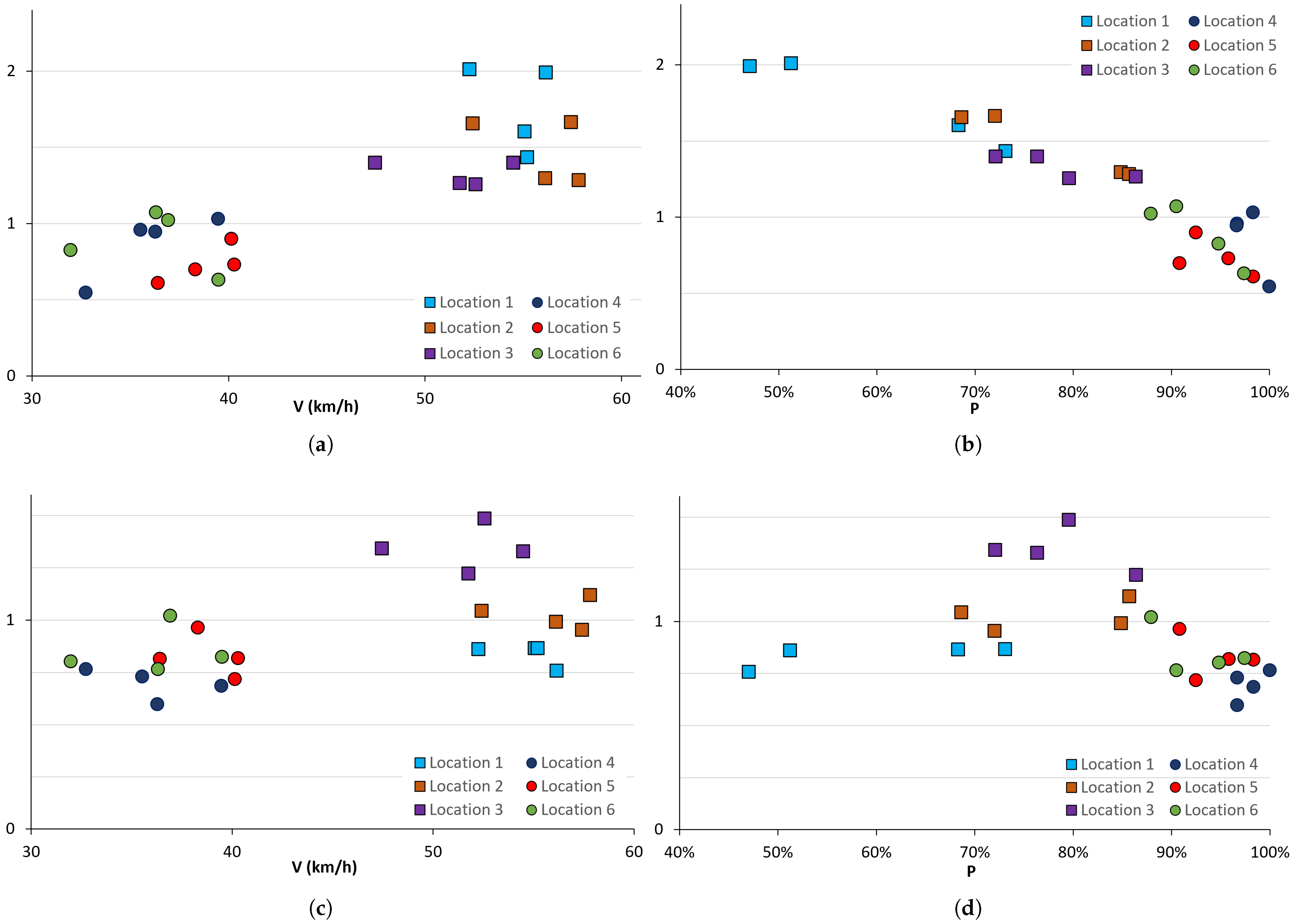
Figure 2 shows the relationship between the estimated parameters of the shifted-lognormal distribution, $\widehat{\mu }$ and ${\widehat{\sigma }}^2$, the average vehicle speed within a group (V) and the share of vehicles travelling in platoons within a group (P). Different markers are used to distinguish groups originating from different observation locations.

Figure 2. Scatter plots of (a) $\widehat{\mu }$ versus V, (b) $\widehat{\mu }$ versus P, (c) ${\widehat{\sigma }}^2$ versus V, and (d) ${\widehat{\sigma }}^2$ versus P for the 24 independent groups considered in the analysis. Different markers are used to distinguish locations where the groups belong.

The results presented in Figure 2 and Table 6 indicate a strong negative relationship between parameter $\widehat{\mu }$ and platoon share P both for the complete dataset and for the two location subsets considered separately. In contrast, the relationship between average vehicle speed V and parameter $\widehat{\mu }$ is strong only when all locations are analysed together, whereas it becomes negligible within the two location subsets (locations 1–3 and locations 4–6). This suggests that the overall correlation is primarily associated with differences between the two groups of locations. The relationship between parameter ${\widehat{\sigma }}^2$ and the explanatory variables appears substantially weaker. Nevertheless, Figure 2d suggests the possible existence of a quadratic relationship between parameter ${\widehat{\sigma }}^2$ and platoon share P. Consequently, both linear and quadratic regression models were considered in the subsequent analysis.

Figure 2 also indicates a clear separation between groups originating from locations 1, 2, and 3, characterized by higher average speeds and lower platoon shares, and groups originating from locations 4, 5, and 6, characterized by lower average speeds and higher platoon shares. Within both location subsets, the strong relationship between platoon share P and parameter $\widehat{\mu }$ remains preserved, whereas the relationship between average speed V and parameter $\widehat{\mu }$ becomes negligible (Table 6). These observations motivated the development of separate models based on data from all locations, locations 1–3, and locations 4–6.

Based on the preceding analysis, models for estimating each of the shifted-lognormal parameters, $\widehat{\mu }$, ${\widehat{\sigma }}^2$, and $\widehat{\tau }$, were sought among the candidate regression models M1–M8 presented in Table 7.

Table 7. Candidate regression models used for estimating the parameters of the shifted-lognormal distribution.

Model	Regression Parameters	General Form
M1	P	$y={\beta }_0+{\beta }_1·P+ϵ$,
M2	V	$y={\beta }_0+{\beta }_1·V+ϵ$,
M3	$P,V$	$y={\beta }_0+{\beta }_1·P+{\beta }_2·V+ϵ$,
M4	P, $P^2$	$y={\beta }_0+{\beta }_1·P+{\beta }_2·P^2+ϵ$,
M5	V, $V^2$	$y={\beta }_0+{\beta }_1·V+{\beta }_2·V^2+ϵ$,
M6	P, $P^2$, V	$y={\beta }_0+{\beta }_1·P+{\beta }_2·P^2+{\beta }_3·V+ϵ$,
M7	P, V, $V^2$	$y={\beta }_0+{\beta }_1·P+{\beta }_2·V+{\beta }_3·V^2+ϵ$,
M8	P, $P^2$, V, $V^2$	$y={\beta }_0+{\beta }_1·P+{\beta }_2·P^2+{\beta }_3·V+{\beta }_4·V^2+ϵ$.

The candidate regression models were compared using standard model-selection criteria [26], namely MSE, PRESS, AIC, AICc, GCV, and BIC. Table 8 presents, for each dataset considered, the model preferred according to a particular selection criterion (strictly speaking, each model should be identified by specifying both the dependent variable, i.e., the shifted-lognormal parameter ($\widehat{\mu }$, ${\widehat{\sigma }}^2$, or $\widehat{\tau }$), and the dataset used for model estimation (all locations, locations 1–3, or locations 4–6). For example, model M1 listed in the first row of Table 8 should formally be denoted as M1$(\widehat{\mu },\mathrm{ALL})$. However, since the corresponding parameter and dataset are evident from the table structure, the simplified notation M1 is used throughout the paper).

Table 8. Best-performing regression models according to the model-selection criteria MSE, PRESS, GCV, AIC, AICc, and BIC for estimation of the shifted-lognormal parameters $\widehat{\mu }$, ${\widehat{\sigma }}^2$, and $\widehat{\tau }$ using data from all locations, locations 1–3, and locations 4–6.

Locations	Parameter	MSE	PRESS	GCV	AIC	AICc	BIC
All	$\widehat{\mu }$	M3	M3	M3	M3	M3	M3
	${\widehat{\sigma }}^2$	M8	M4	M4	M4	M4	M4
	$\widehat{\tau }$	M4	M4	M4	M4	M4	M4
1, 2, and 3	$\widehat{\mu }$	M3	M1	M3	M3	M1	M3
	${\widehat{\sigma }}^2$	M3	M3	M3	M3	M3	M3
	$\widehat{\tau }$	M6	M3	M2	M2	M2	M2
4, 5, and 6	$\widehat{\mu }$	M1	M1	M1	M1	M1	M1
	${\widehat{\sigma }}^2$	M1	M1	M1	M1	M1	M1
	$\widehat{\tau }$	M1	M1	M1	M1	M1	M1

The model-selection results presented in Table 8 indicate a high degree of agreement among the selection criteria for most of the considered cases. When several models produced similar performance, preference was given to the simpler model with fewer explanatory terms. The resulting models provide a compromise between goodness of fit and model parsimony and were therefore selected for further analysis. Visual inspection of the regression residuals did not reveal systematic patterns that would indicate substantial model misspecification within the observed operating range. Furthermore, all selected regression equations yield positive estimates of the variance parameter ${\widehat{\sigma }}^2$ within the range of vehicle speeds and platoon shares observed in the study dataset.

Based on the results shown in Table 8, the following models were selected for estimating the parameters of the shifted-lognormal distribution using data from all locations:

$${\mathrm{PM}}^{\mathrm{ALL}}\dots \left\{\begin{array}{c}\widehat{\mu }=2.543-2.147·P+0.0096·V,\hfill \\ {\widehat{\sigma }}^2=-5.548+18.811·P-12.890·P^2,\hfill \\ \widehat{\tau }=-2.546+7.904·P-5.397·P^2.\hfill \end{array}\right.$$

The single-regime model ${\mathrm{PM}}^{\mathrm{ALL}}$ serves as a reference model obtained from the complete dataset.

If only the data from locations 1, 2, and 3 are considered, the model selected on the basis of the model-selection criteria is:

$${\mathrm{PM}}^{123}\dots \left\{\begin{array}{c}\widehat{\mu }=2.998-2.050·P,\hfill \\ {\widehat{\sigma }}^2=4.679+2.415·P-0.0967·V,\hfill \\ \widehat{\tau }=3.663-0.0625·V,\hfill \end{array}\right..$$

On the other hand, if only the data from locations 4, 5, and 6 are considered, the model selected on the basis of the model-selection criteria is:

$${\mathrm{PM}}^{456}\dots \left\{\begin{array}{c}\widehat{\mu }=3.007-2.266·P,\hfill \\ {\widehat{\sigma }}^2=3.135-2.660·P,\hfill \\ \widehat{\tau }=-0.100+0.180·P,\hfill \end{array}\right..$$

The shift parameter $\widehat{\tau }$ exhibited substantially weaker correlations with the explanatory variables than parameter $\widehat{\mu }$. Consequently, the regression equations for $\widehat{\tau }$ should be interpreted with greater caution, particularly near the boundaries of the observed ranges of V and P. Small negative estimates of $\widehat{\tau }$ may occur near these boundaries, indicating that the corresponding time-headway distribution is adequately approximated by a standard lognormal distribution. In practical applications, negative values of $\widehat{\tau }$ may therefore be replaced by zero, resulting in a standard lognormal distribution.

5. Internal Assessment of the Proposed Models

The next step is to assess how well the shifted-lognormal distributions obtained from the proposed regression models represent the observed time-headway data.

First, the traffic-flow characteristics P and V are calculated from the observed data. Second, the parameters of the shifted-lognormal distribution are estimated using the selected regression model and the corresponding values of P and V. Finally, the Kolmogorov–Smirnov goodness-of-fit test is applied to evaluate the agreement between the observed time-headway data and the fitted shifted-lognormal distribution.

Algorithm 2 describes the procedure used to assess whether a given set of observed time headways can be represented by a shifted-lognormal distribution whose parameters are obtained from the regression model M.

The purpose of this procedure is to assess the agreement between the observed and model-based distributions for the analysed datasets rather than to provide an independent external validation of the proposed models. Furthermore, it should be noted that the generated assessment samples are not statistically independent because they originate from the same observation locations and partially overlap. Consequently, the acceptance percentages reported in this section should be interpreted only as indicators of agreement between the observed and model-based distributions within the available dataset and not as measures of external predictive performance.

Algorithm 2 Assessment of model-based shifted-lognormal distributions.
Input: vehicle time-headway observations $X=\{x_1,x_2,\dots ,x_n\}$, M—mathematical model, $\alpha$—given level of significance.
S0:	Start
S1:	For sample X calculate the mean vehicle speed, V, and the share of vehicles in platoons in the sample, P.
S2:	From model M, based on values V and P, calculate estimates $\mu$, ${\sigma }^2$ and $\tau$.
S3:	Let $L\sim \mathrm{\Lambda }(\mu ,{\sigma }^2,\tau )$ be a shifted-lognormal distribution.
S4:	Let $D(\mu ,{\sigma }^2,\tau )$ denote the value of Kolmogorov–Smirnov statistic which measures the distance between the empirical distribution function of sample X and shifted-lognormal distribution L,
S5:	If $D\left(\mu ,{\sigma }^2,\tau \right)$ is lower than the critical value of the Kolmogorov–Smirnov test, the hypothesis that sample X is consistent with distribution L cannot be rejected.
S6:	End

To assess the consistency of the proposed models, a set of additional test samples was generated from each observation location.

The generation of test samples requires special care because the temporal ordering of vehicles directly affects the observed headway sequence and must therefore be preserved. Accordingly, each test sample consists of a sequence of consecutive vehicles. For any given location, the k samples of size L are generated using the following procedure:

• Let $A=\{A_1,A_2,\dots ,A_N\}$ denote the sequence of vehicles observed at a given location;
• Let the length of sample L be given, and let k be the wanted number of samples of a given length. Samples $S_1,\dots ,S_k$ need to be generated;
• The first sample $S_1$ consists of the first L consecutive elements in A, whereas the last sample $S_k$ consists of the last L consecutive elements in A; $S_1=\{A_1,\dots ,A_L\}$ and $S_k=\{A_{N-L+1},\dots ,A_N\}$, and
• Sample $S_j$, $j=2,\dots ,k-1$ consists of consecutive elements $A_{(j-1)·s+1},\dots ,A_{(j-1)·s+L}$, where $s=(N-L)/(k-1)$.

This procedure ensures that each test sample contains temporally consecutive vehicles while providing a broad coverage of the observed traffic stream.

In this way, 150 samples were generated for the data from each location (15 samples for each size from 100 to 275 vehicles, and 10 samples for the sizes 300, 325, and 350 vehicles). Table 9 presents the results of the internal evaluation procedure described in Algorithm 2. The procedure was carried out with two levels of significance (5% and 1%) and on the samples generated from the data from all locations. In addition to the aggregated results, samples originating from locations 1–3 and locations 4–6 were analysed separately.

Table 9. Results of the model-based internal evaluation procedure. Columns Sig. 5% and Sig. 1% indicate the proportion of samples satisfying the acceptance criterion of Algorithm 2 at significance levels of 5% and 1%, respectively. Results are shown for all generated samples and separately for samples originating from locations 1–3 and locations 4–6.

	All Locations		Locations 1, 2, and 3		Locations 4, 5, and 6
Model	Sig. 5%	Sig. 1%	Sig. 5%	Sig. 1%	Sig. 5%	Sig. 1%
${\mathrm{PM}}^{\mathrm{ALL}}$	58.2%	77.4%	62.0%	80.7%	54.4%	74.2%
${\mathrm{PM}}^{123}$	39.0%	44.1%	78.0%	88.2%	0.0%	0.0%
${\mathrm{PM}}^{456}$	37.6%	47.6%	4.4%	15.1%	70.7%	80.0%

The results presented in Table 9 indicate that the proposed models exhibit different levels of agreement with the observed data depending on the traffic regime for which they were developed. The single-regime model ${\mathrm{PM}}^{\mathrm{ALL}}$ provides a moderate level of agreement across the entire dataset, achieving acceptance rates between 58.2% and 77.4%, depending on the selected significance level. In contrast, the regime-specific models exhibit substantially better performance when applied to samples originating from the corresponding group of locations. Model ${\mathrm{PM}}^{123}$ achieves acceptance rates of 78.0% and 88.2% for samples generated from locations 1–3, whereas its performance on samples from locations 4–6 is negligible. Similarly, model ${\mathrm{PM}}^{456}$ achieves acceptance rates of 70.7% and 80.0% for samples originating from locations 4–6, while showing poor agreement with samples from locations 1–3.

These results further support the distinction between two traffic regimes characterized by different combinations of average vehicle speed and platoon share. Furthermore, they indicate that the regime-specific models provide better agreement with the observed time-headway distributions within their respective traffic conditions than a single model estimated from the complete dataset.

6. Conclusions

The statistical properties of vehicle arrival headways were investigated using detailed traffic observations collected at six urban motorway locations in the City of Zagreb, including open motorway sections, a tunnel, a bridge, and an underpass. The collected dataset enabled the determination of individual vehicle speeds, time headways, and derived space headways from frame-by-frame analysis of video recordings. The analysis showed that the observed headway data can be adequately represented by shifted-lognormal distributions. Furthermore, the investigated locations exhibited two distinct traffic operating regimes. The first regime was characterised by higher average vehicle speeds and lower shares of vehicles travelling in platoons, whereas the second regime was characterised by lower average speeds and higher platoon shares.

Regression models were developed to estimate the parameters of the shifted-lognormal distribution using two explanatory variables: average vehicle speed and the share of vehicles travelling in platoons. Comparison of alternative regression formulations showed that simple relationships between the distribution parameters and traffic-flow characteristics can be established. The results also indicate that a single model developed from the complete dataset does not provide the same level of agreement with the observed data as models developed separately for the two identified traffic regimes. The internal evaluation procedure demonstrated that regime-specific models provide a substantially better representation of headway distributions when applied within the corresponding traffic regime. This finding supports the use of a multi-regime approach for modelling vehicle arrival headways under different traffic operating conditions.

The proposed models should be interpreted within the range of traffic conditions represented by the analysed dataset. Although the models were developed using observations collected at six locations, the identified relationships between headway-distribution parameters, average vehicle speed, and platoon share provide a useful framework for describing traffic streams operating under similar conditions. Future research should include observations from additional locations and a wider range of traffic conditions in order to further examine the stability of the identified traffic regimes and to refine the proposed regression models. The present study does not propose a formal classification rule for assigning previously unobserved traffic streams to a particular regime. Instead, the identified regimes should be interpreted as descriptive categories derived from the six investigated locations. Particular attention should be devoted to the development of operational criteria for regime assignment and to the validation of such criteria using additional locations and traffic conditions.

References

- Elefteriadou, L. An Introduction to Traffic Flow Theory; Springer: New York, NY, USA, 2014; pp. 65–68. [Google Scholar] [CrossRef] [Scilit]
- Cantisani, G.; Del Serrone, G.; Mauro, R.; Peluso, P.; Pompigna, A. Traffic stream analysis by radar sensors on two-lane roads for free-moving and constrained vehicles identification. Sensors 2023, 23, 6922. [Google Scholar] [CrossRef] [Scilit]
- Roy, R.; Saha, P. Microscopic Analysis of Time Headway of Vehicles on Two-Lane Highways with Mixed Traffic. SN Comput. Sci. 2023, 4, 287. [Google Scholar] [CrossRef] [Scilit]
- Horvat, R.; Kos, G.; Ševrović, M. Traffic flow modelling on the road network in the cities. Teh. Vjesn. Tech. Gaz. 2015, 2, 475–486. [Google Scholar] [CrossRef] [Scilit]
- Drew, D.R. Traffic Flow Theory and Control; McGraw-Hill Book Company: New York, NY, USA, 1968. [Google Scholar]
- Greenshields, B.D. A Study of Traffic Capacity. Proc. Highw. Res. Board 1934, 14, 448–477. [Google Scholar] [CrossRef] [Scilit]
- Greenberg, H. An Analysis of Traffic Flows. Oper. Res. 1959, 7, 79–85. [Google Scholar] [CrossRef] [Scilit]
- Underwood, R. Speed, Volume and Density Relationships. Qual. Theory Traffic Flow. 1960, 141–188. [Google Scholar]
- May, A.D. Traffic Flow Fundamentals; Prentice Hall: Englewood Cliffs, NJ, USA, 1990; pp. 338–375. [Google Scholar]
- Buckley, D. A semi-poisson model of traffic flow. Transp. Sci. 1968, 2, 107–133. [Google Scholar] [CrossRef] [Scilit]
- Cowan, R.J. Useful headway models. Transp. Res. 1975, 9, 371–375. [Google Scholar] [CrossRef] [Scilit]
- Zhang, G.; Wang, Y.; Wei, H.; Chen, Y. Examining headway distribution models with urban freeway loop event data. Transp. Res. Rec. 2007, 1999, 141–149. [Google Scholar] [CrossRef] [Scilit]
- Ha, D.H.; Aron, M.; Cohen, S. Time headway variable and probabilistic modeling. Transp. Res. Part C Emerg. Technol. 2012, 25, 181–201. [Google Scholar] [CrossRef] [Scilit]
- Li, L.; Chen, X. Vehicle headway modeling and its inferences in macroscopic/microscopic traffic flow theory: A survey. Transp. Res. Part C Emerg. Technol. 2017, 76, 170–188. [Google Scholar] [CrossRef] [Scilit]
- Vogel, K. What Characterizes a “free Vehicle” in an Urban Area? Transp. Res. Part F Traffic Psychol. Behav. 2002, 5, 15–29. [Google Scholar] [CrossRef] [Scilit]
- Transportation Research Board. Highway Capacity Manual, 5th ed.; Transportation Research Board: Washington, DC, USA, 2010. [Google Scholar]
- Shiomi, Y.; Yoshii, T.; Kitamura, R. Platoon-Based Traffic Flow Model for Estimating Breakdown Probability at Single-Lane Expressway Bottlenecks. Procedia Soc. Behav. Sci. 2011, 17, 591–610. [Google Scholar] [CrossRef] [Scilit]
- Badhrudeen, M.; Ramesh, V.; Vanajakshi, L. Headway analysis using automated sensor data under Indian traffic conditions. Transp. Res. Procedia 2016, 17, 331–339. [Google Scholar] [CrossRef] [Scilit]
- Kajalić, J.; Čelar, N.; Stanković, S.; Kocić, A. Vehicle Platoon Membership Definition for Unsaturated Conditions. Int. J. Traffic Transp. Eng. 2021, 11, 199. [Google Scholar] [CrossRef] [Scilit]
- Mauro, R.; Pompigna, A. A Statistically Based Model for the Characterization of Vehicle Interactions and Vehicle Platoons Formation on Two-Lane Roads. Sustainability 2022, 14, 4714. [Google Scholar] [CrossRef] [Scilit]
- Kasi, K.; Karuppanan, G. Framework to Identify Vehicle Platoons under Heterogeneous Traffic Conditions on Urban Roads. Sustainability 2024, 16, 724. [Google Scholar] [CrossRef] [Scilit]
- Pompigna, A.; Cantisani, G.; Del Serrone, G. Probabilistic Modeling of Inter-Vehicle Spacing on Two-Lane Roads: Implications for Safety-Oriented and Sustainable Traffic Operations. Sustainability 2026, 18, 2896. [Google Scholar] [CrossRef] [Scilit]
- Greenberg, I. The log-normal distribution of headways. Austral. Road Res. 1966, 2, 13–17. [Google Scholar]
- Crow, E.L.; Shimizu, K. Lognormal Distributions: Theory and Applications; Dekker: New York, NY, USA, 1988. [Google Scholar]
- Krishnamoorthy, K. Handbook of Statistical Distributions with Applications; Chapman and Hall/CRC: Boca Raton, FL, USA, 2006. [Google Scholar]
- Yan, X.; Su, X.G. Linear Regression Analysis: Theory and Computing; World Scientific: Singapore, 2009; pp. 157–195. [Google Scholar]
Disclaimer/Publisher’s Note: The statements, opinions and data contained in all publications are solely those of the individual author(s) and contributor(s) and not of MDPI and/or the editor(s). MDPI and/or the editor(s) disclaim responsibility for any injury to people or property resulting from any ideas, methods, instructions or products referred to in the content. |
© 2026 by the authors. Licensee MDPI, Basel, Switzerland. This article is an open access article distributed under the terms and conditions of the Creative Commons Attribution (CC BY) license.