Isotropic Coordinate Normalization and Target-Aware Search for Vehicle Trajectory Clustering at Complex Urban Intersections

Abstract

Grouping vehicles with similar paths is important for traffic analysis, but camera-image trajectories are distorted by perspective, and unsupervised clustering does not directly reveal how many traffic movements should be expected. This paper presents Homography-Guided Semantic Maneuver Graph Trajectory Clustering (HG-SMG-TC), a model-selection framework that uses a lightweight homography to estimate intersection structure while retaining isotropically normalized camera coordinates for clustering. Entry and exit endpoint groups are consolidated into physical approach-level groups, and their supported origin–destination relationships form a maneuver graph. Bootstrap resampling converts this structure into an interval for the expected number of observed movements, which guides clustering model selection. The method is evaluated on 67,029 vehicle trajectories from five urban intersection scenes in the Traffic Node Video Dataset, using separate target-estimation, model-selection, and independent-test recording blocks. Independent polygon-rule reference labels cover 89.6–98.4% of test trajectories. HG-SMG-TC reduces mean target-count error from 3.20 for untargeted selection and 2.53 for the point-target variant to 2.13, while achieving an adjusted Rand index of 0.734 and normalized mutual information of 0.839. The results show that the proposed semantic maneuver prior improves target alignment and provides a reproducible way to guide unsupervised trajectory clustering, while retaining explicit trade-offs across evaluation metrics.

1. Introduction

1.1. Traffic-Video-Based Trajectory Analysis

Traffic management systems and intelligent transportation systems are important and dynamically developing areas of transport infrastructure. The number of cameras installed in road environments has increased considerably over the last decade, and this trend has been accompanied by the rapid development of image processing, object detection, tracking, and artificial-intelligence-based interpretation methods. These technologies make it possible to use visual information not only for manual surveillance, but also for traffic analysis, safety monitoring, transport planning, and modelling.

Recent international work shows that camera-based trajectory extraction is moving from isolated local experiments toward large-scale, network-level traffic sensing. Traffic-camera trajectory recovery has been formulated at road-network and intersection granularity, with iterative re-identification and trajectory-recovery pipelines used to reconstruct vehicle movements from sparse and heterogeneous camera observations [1]. City-scale trajectory datasets recovered from thousands of cameras have also been published, confirming that video-based trajectories are becoming an important data source for traffic surveillance, prediction and control [2]. More recent recovery frameworks, including TrajRecovery and VisionTraj, further indicate a shift toward scalable, noise-robust and learning-based reconstruction from camera records and visual snapshots [3,4].

These developments also highlight a practical limitation that is directly relevant to the present paper: trajectory data obtained from traffic video require careful geometric processing, validation and task-aware interpretation. Recent reviews on computer-vision-based trajectory generation for traffic safety emphasize that detection and tracking are only the first stages; video preprocessing, post-processing, trajectory reconstruction and validation strongly influence the usability of the extracted data [5]. Similarly, recent CCTV-based studies still use bird’s-eye-view transformation and homography for high-resolution traffic data extraction, while noting that calibration quality remains a key practical constraint [6].

Urban intersections are particularly relevant scenes for this type of analysis. Compared with highway traffic, urban traffic contains frequent acceleration and deceleration, turning movements, lane changes, and interactions between several transport actors. For this reason, camera-based trajectories extracted at intersections contain valuable information about the actual movement structure of the scene. Previous work on the Traffic Node Video Dataset presented video recordings and processed trajectory data for eight intersections, together with filtering, filling, and Python-based examples for trajectory modelling [7]. Further studies used YOLOv7-based object detection, DeepSORT tracking, and trajectory clustering to generate street-level or lane-level traffic statistics from the same video recordings [8,9].

A practical design question in traffic-camera-based trajectory analysis is how much geometric calibration is necessary for a given task. At one extreme, all processing can be performed directly in the image plane of the camera. This solution is simple and calibration-free, but the resulting trajectory geometry is affected by perspective distortion and does not explicitly represent the road-plane structure of the intersection. At the other extreme, recent works show that traffic-camera analysis can be supported by more advanced metric, 3D, or multi-camera calibration. For example, Zhang et al. used 2D homography to transform CCTV camera views into bird’s-eye-view representations for high-resolution traffic data collection, including vehicle trajectories, speed and acceleration estimation [6]. Campos Ruiz et al. proposed panoramic image-based 3D scene reconstruction for automated traffic camera calibration, emphasizing focal length estimation, localization precision and ground-plane consistency [10]. Song et al. applied multicamera calibration and 3D trajectory reconstruction to support cross-camera vehicle tracking and long-distance trajectory association in complex traffic scenes [11]. These studies demonstrate the value of calibrated geometric representations, but they also show that calibration effort, required scene information and scalability remain important practical considerations. The present study is positioned between image-plane-only processing and full metric or 3D reconstruction: it uses a lightweight planar homography as a geometric reference for estimating the observed maneuver structure, while the final clustering representation remains simple and computationally practical.

1.2. Trajectory Clustering and the Model-Selection Problem

Automatically grouping vehicles that follow similar paths is a basic task in traffic-video analysis. The difficulty is that trajectories measured directly in camera-image coordinates are affected by perspective distortion: equal physical displacements can appear very different depending on their location in the image. At the same time, an unsupervised clustering algorithm does not know in advance how many meaningful traffic movements are present at an intersection. The present work addresses these two related problems by separating geometric scene interpretation from the final clustering representation.

Trajectory clustering is a natural step between raw vehicle tracks and higher-level traffic interpretation. By grouping vehicles according to their entry and exit regions, it is possible to identify maneuver-like groups such as straight movements, right turns, and left turns. Such groups can support traffic statistics, anomaly detection, and later trajectory prediction tasks. However, the practical performance of trajectory clustering depends not only on the clustering algorithm, but also on feature representation, coordinate normalization, and parameter selection.

The recent trajectory-clustering literature has therefore moved beyond a single fixed distance-and-clustering recipe. Dynamic representation learning has been proposed to reduce dependence on manually designed trajectory similarity measures and to improve clustering of large-scale vehicle trajectories [12]. Other recent work focuses on efficient density-based clustering of continuous trajectories in road networks, showing that scalability and representation remain central challenges when trajectories are treated as spatiotemporal objects [13]. In traffic-video settings, smart-intersection studies continue to compare distance measures, evaluation scores and trajectory-clustering setups for estimating street-to-street traffic movement [14].

A particularly important methodological result is that trajectory clustering does not have a universally best algorithm, distance measure or validation metric. Rezaie and Saunier proposed automatically generated origin–destination reference clusters for evaluation without manual trajectory labels and showed that the best-performing setup depends on the intersection and evaluation objective [15]. This motivates the present study: rather than replacing established clustering algorithms, the proposed framework focuses on geometry-aware prior construction, coordinate representation, and reproducible model selection.

Classical internal clustering metrics, including the silhouette coefficient and the Davies–Bouldin index, measure compactness and separation [16,17]. These metrics are useful, but they do not directly encode the traffic interpretation objective. A mathematically compact partition can merge two traffic movements, while an over-fragmented solution can split one observed maneuver into several artificial subgroups. This creates a blind spot in unsupervised traffic-scene analysis: the clustering result must be evaluated not only as a point-cloud partition, but also as a representation of the maneuver structure of the intersection.

1.3. Research Gap, Objective and Contribution

Several related problems have already been studied. Previous methods can detect entry and exit regions from trajectory endpoints and derive origin–destination (OD) movements from them [18,19]. Other approaches use trajectory geometry to reconstruct lanes, road structure, or movement graphs [20,21,22,23,24], while multi-criteria methods have been proposed for selecting among alternative trajectory clusterings [25]. These results provide useful building blocks, but they leave an important model-selection problem unresolved.

In practice, vehicles belonging to the same physical road approach can form several separate endpoint groups due to lane structure, perspective, or normal variation in their paths. Counting all of these geometric groups directly can therefore overestimate the number of meaningful traffic movements and force the clustering toward too many clusters. This is the specific problem addressed in this paper.

We propose Homography-Guided Semantic Maneuver Graph Trajectory Clustering (HG-SMG-TC). The method first identifies geometric groups of entry and exit endpoints, then merges compatible groups representing the same physical approach. Their supported OD relations form a maneuver graph. Repeated bootstrap sampling is then used to estimate a range, rather than a single fixed value, for the expected number of observed movements. This interval is used to guide unsupervised model selection. Importantly, the reference labels used for the final evaluation are kept completely separate from this process. Here, semantic refers to the physical traffic meaning of an approach-level group; no manually assigned semantic label is used during the consolidation step.

To the best of our knowledge, this complete combination of homography-supported endpoint grouping, label-free approach consolidation, maneuver-graph construction, bootstrap-based target uncertainty, and interval-constrained clustering model selection has not previously been reported for fixed-camera vehicle trajectory clustering.

The main contributions are:

• A new HG-SMG-TC model-selection method that distinguishes small geometric endpoint groups from traffic-meaningful road approaches and uses an interval rather than a single expected cluster count;
• A three-way evaluation protocol that separates target estimation, model selection, and independent testing by complete recording blocks, preventing reference information from influencing clustering;
• An independent polygon-rule reference that enables evaluation with cluster-count error, adjusted Rand index, and normalized mutual information, purity, precision, recall, and F1 scores;
• Sensitivity analyses for homography calibration, maneuver-target estimation, reference construction, and the task-specific Expected-Maneuver Alignment Score;
• Evaluation on five Bellevue intersections, including simple endpoint and trajectory-shape baselines and a detailed analysis of the main failure mode of the point-target approach.

2. Materials and Methods

2.1. Overview of the HG-SMG-TC Workflow

HG-SMG-TC separates two tasks that should not necessarily use the same coordinate representation. Final trajectory clustering is performed in isotropically normalized camera coordinates, while a planar homography is used only to obtain a simplified top-view representation of the intersection for estimating its movement structure.

The first step identifies compact geometric groups among entry and exit endpoints. We refer to such a group as an endpoint micro-mode. A micro-mode may represent a lane, a lane group, or another local concentration of endpoints; it is therefore not assumed to correspond to a complete traffic movement. This distinction is central to the proposed method. Compatible micro-modes are subsequently combined into approach-level groups before the expected maneuver structure is estimated.

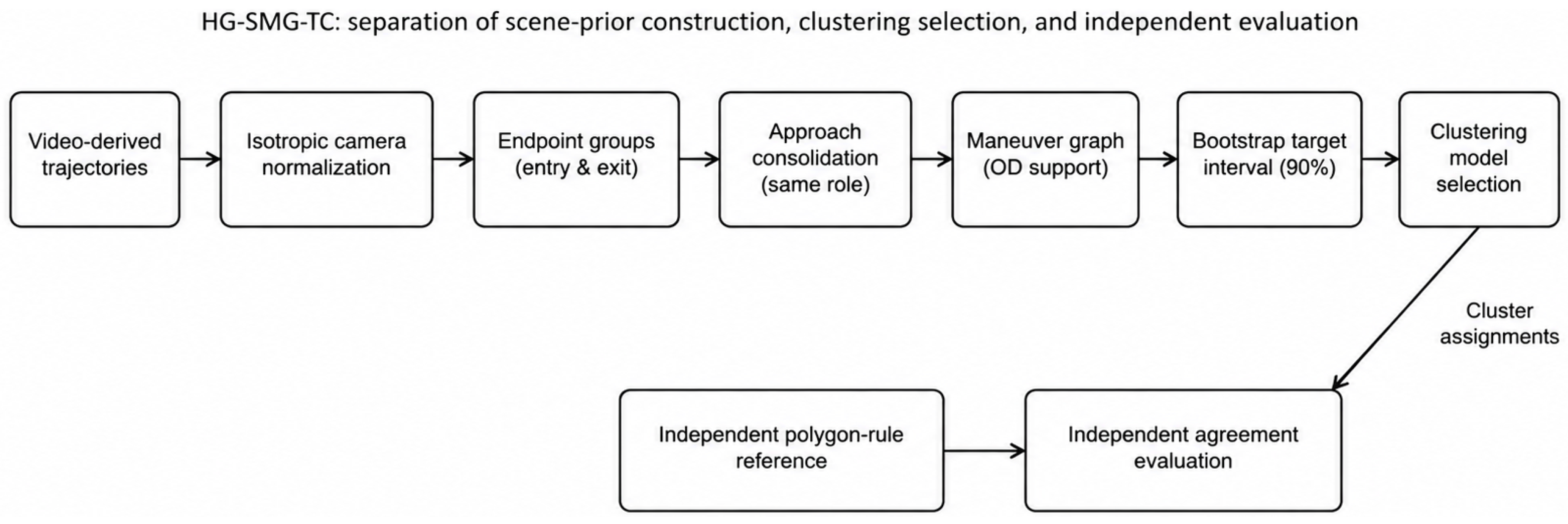
The workflow has five functional stages: (i) video-derived trajectories are cleaned and represented in isotropically normalized camera coordinates; (ii) homography-transformed endpoints are partitioned into entry and exit endpoint groups; (iii) compatible groups belonging to the same role are consolidated into approach-level groups, and their origin–destination (OD) support is aggregated into a maneuver graph; (iv) recording-aware bootstrap resampling produces an interval for the plausible number of observed maneuvers, which is used to constrain clustering configuration selection; and (v) the selected configurations are refit on the unlabeled independent-test trajectories and evaluated only after all cluster assignments have been saved.

Three comparison variants are used throughout the experiments. A0 denotes untargeted model selection based only on the predefined clustering-quality criteria. A1 adds the homography-derived geometric endpoint-pair count as a single target value. A5 denotes the complete HG-SMG-TC method, in which compatible endpoint groups are consolidated, a maneuver graph is constructed, and bootstrap uncertainty is propagated into interval-constrained model selection. The A0, A1, and A5 labels are retained in figures and tables for compactness.

2.2. Dataset, Trajectory Representation and Split Protocol

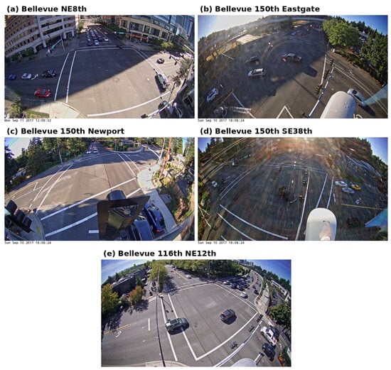
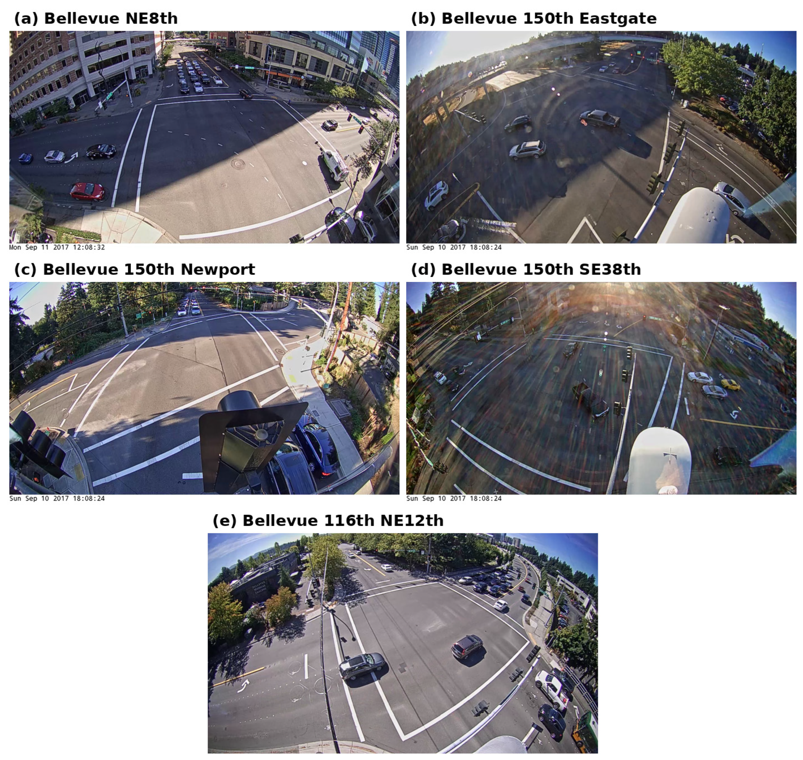
The Traffic Node Video Dataset contains eight traffic-video locations. This paper uses the five Bellevue intersections from that dataset as a consistent multi-scene evaluation subset: bellevue_ne8th, bellevue_150th_eastgate, bellevue_150th_newport, bellevue_150th_se38th, and bellevue_116th_ne12th. These sites are urban, signalized, multi-approach intersections with visibly different camera viewpoints, approach geometries, and turning-movement distributions. The subset therefore provides a practical testbed for evaluating whether trajectory clustering model selection can be made more consistent across related but non-identical urban scenes. The five selected intersections are shown in Figure 1.

Figure 1. Representative video frames from the five Bellevue intersections used in this study: (a) Bellevue NE8th; (b) Bellevue 150th/Eastgate; (c) Bellevue 150th/Newport; (d) Bellevue 150th/SE38th; (e) Bellevue 116th/NE12th.

In this study, cleaned trajectory data refers to vehicle trajectories after the preprocessing workflow has filtered, repaired, and post-processed the raw tracking output. The cleaning stage removes noisy, fragmented, very short, or otherwise unreliable tracks; keeps reliable vehicle-only trajectories; and applies gap filling, smoothing, and trimming as defined by the data-processing workflow. These cleaned trajectories are then used for feature generation, coordinate normalization, homography-based endpoint transformation, and clustering.

$$x=[x_s, y_s, x_e, y_e],$$

(1)

For clustering, each cleaned trajectory is represented by its start and end coordinates, where the subscripts s and e denote the start and end points, respectively. Camera coordinates are normalized with one shared scale rather than independently by axis. The shared normalization scale d is defined as

$$d=max(x_{\mathrm{m}\mathrm{a}\mathrm{x}}-x_{min}, y_{max}-y_{min}),$$

(2)

$$x^{\prime }={\displaystyle \frac{x-x_{\mathrm{m}\mathrm{i}\mathrm{n}}}{d}}, y^{\prime }={\displaystyle \frac{y-y_{\mathrm{m}\mathrm{i}\mathrm{n}}}{d}}$$

(3)

This isotropic normalization preserves the camera-plane aspect ratio and therefore preserves endpoint directions and relative geometry. Normalization parameters are estimated from the unlabeled trajectories of the corresponding analysis split; reference labels are never used to determine them.

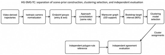
The 67,029 canonical trajectories were divided by complete recording blocks into three non-overlapping subsets: 19,924 trajectories for target estimation, 19,712 for clustering model selection, and 27,393 for independent testing. Complete source recordings were kept intact to prevent temporally adjacent fragments from crossing split boundaries. The split-aware runner further verified that no exact or conservative near-duplicate trajectory candidates crossed the protocol boundaries. Table 1 reports scene-level counts and the independent-reference coverage, while Figure 2 summarizes the complete workflow and the separation between scene-prior construction, clustering model selection, and independent evaluation.

Table 1. Scene-level trajectory counts, split allocation, and independent-reference coverage.

Scene	All	Target Estimation	Model Selection	Test	Valid Reference	Coverage
116th/NE12th	2321	723	634	964	864	89.63%
150th/Newport	9448	2423	3101	3924	3852	98.17%
150th/Eastgate	26,266	8720	6791	10,755	10,586	98.43%
150th/SE38th	9060	2482	2865	3713	3422	92.16%
NE8th	19,934	5576	6321	8037	7510	93.44%
Total	67,029	19,924	19,712	27,393	26,234	95.77%

Figure 2. Overview of the Homography-Guided Semantic Maneuver Graph Trajectory Clustering (HG-SMG-TC) workflow. Endpoint groups are consolidated into approach-level groups, their supported origin-destination relations form a maneuver graph, and bootstrap resampling defines a target interval for model selection. The independent polygon-rule reference is used only for final evaluation.

2.3. Homography Calibration and Geometric Support Layer

For each Bellevue scene, manually selected camera-to-top-view correspondences define a planar projective transformation. The top-view calibration aids originated from scene-matched Google Maps satellite/map-view screenshots. Because acquisition date, zoom level, embedded attribution metadata, and redistribution permission were not preserved with the historical rasters, the raster images are not redistributed as scientific artifacts. Reproducibility is instead supported by the numerical correspondence coordinates, source-image dimensions and hashes, inlier masks, homography matrices, residual summaries, and provenance records.

$${\mathbf{p}}_{\mathrm{c}}=\left[\begin{array}{c}{x}_c\\ y_c\\ 1\end{array}\right]$$

(4)

For a camera point represented in homogeneous coordinates, the planar homography $\mathbf{H}$ maps the point to the top-view reference plane according to

$$\lambda {\mathbf{p}}_{\mathrm{t}}=\mathbf{H}{\mathbf{p}}_{\mathrm{c}}.$$

(5)

where ${\mathbf{p}}_{\mathrm{t}}$ is the corresponding homogeneous top-view point and $\lambda$ is an arbitrary homogeneous scale factor [26]. The homography matrix H is estimated using the RANSAC method [27], as implemented in OpenCV’s findHomography routine of OpenCV 4.12.0 (opencv-python 4.12.0.88), with a 10-pixel destination-space reprojection threshold, a maximum of 2000 iterations, and a confidence level of 0.995. The resulting matrix is normalized by its bottom-right element. No lens-distortion correction is applied. For the NE8th scene, 18 correspondences are used after excluding five previously identified high-error points; the rejected point identifiers remain available in the calibration records.

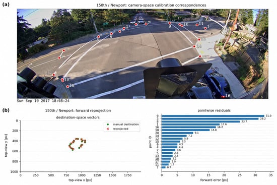
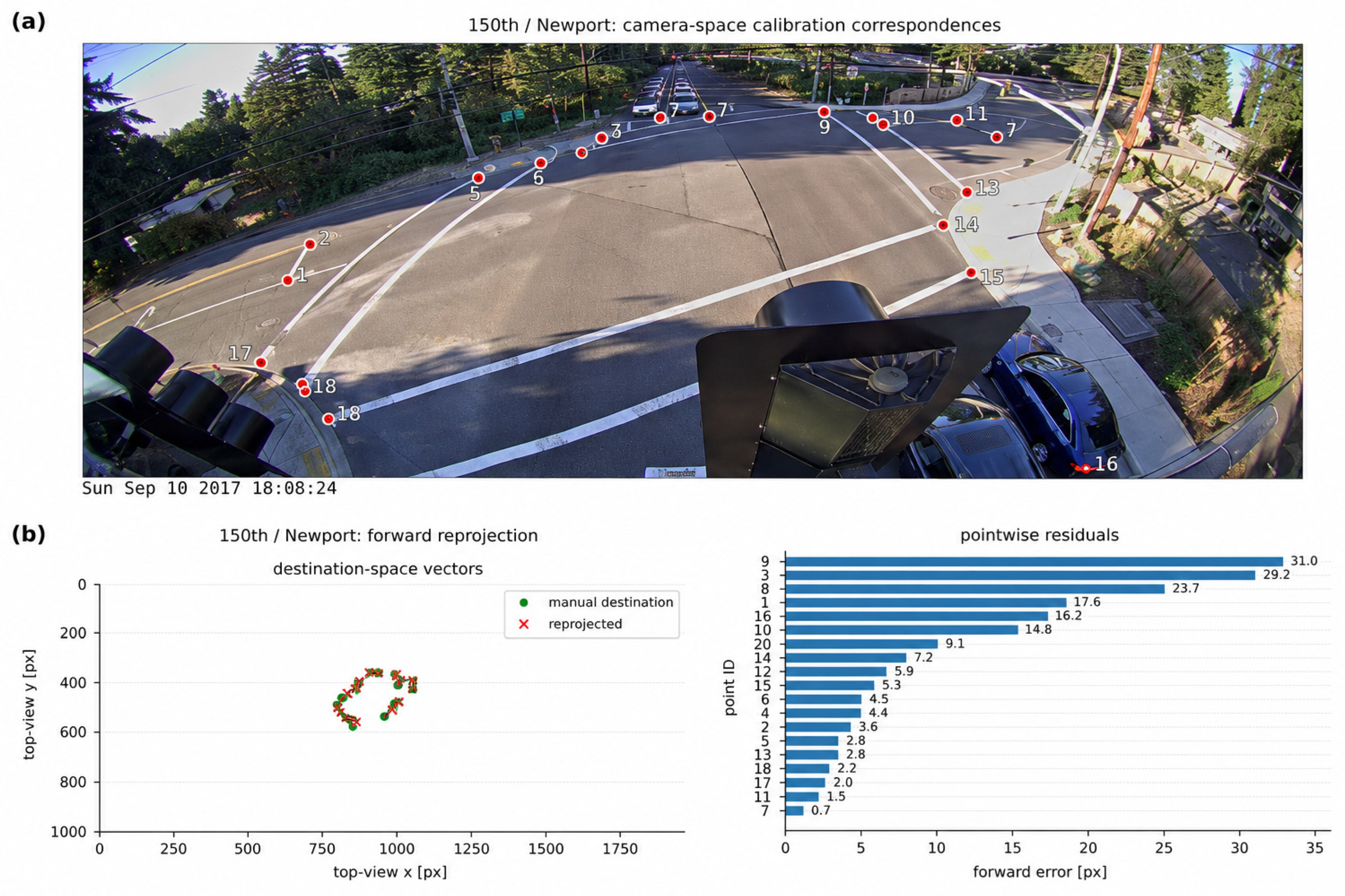
Calibration is evaluated with all-point forward reprojection residuals, normalized RMSE and P95 error relative to the destination-image diagonal, RANSAC inlier fraction, calibration-hull area, and the fraction of target-estimation endpoints outside the source control-point hull. The diagnostic engineering screening classes are defined before clustering/reference evaluation. A scene is good when normalized RMSE ≤ 1%, normalized P95 ≤ 2%, inlier fraction ≥ 60%, source-hull area ≥ 20%, and endpoint extrapolation ≤ 95%; acceptable thresholds are ≤2%, ≤4%, ≥40%, ≥10%, and ≤98%, respectively. A third acceptable-with-caution level uses ≤3%, ≤6%, ≥30%, ≥5%, and ≤99.5%. All criteria of the first matching class must hold. A representative calibration and forward-reprojection diagnostic is shown in Figure 3, while the scene-level calibration diagnostics are summarized in Table 2.

Figure 3. Homography calibration diagnostic for 150th/Newport: (a) camera-space control-point correspondences; (b) destination-space forward reprojection vectors and pointwise residual magnitudes. The third-party top-view raster is not reproduced; the numerical destination coordinates and calibration artifacts are provided for reproducibility. The scene-level calibration diagnostics are summarized in Table 2.

Table 2. Homography calibration quality and endpoint extrapolation. RMSE: root mean square error; P95: 95th percentile.

Scene	Points/ Inliers	RMSE [px]	Normalized RMSE	P95 [px]	Endpoint Extrapolation	Class
116th/NE12th	26/17	23.86	1.16%	41.55	91.98%	acceptable
150th/Newport	20/13	13.02	0.61%	29.31	96.95%	acceptable
150th/Eastgate	13/11	14.61	0.69%	33.77	92.98%	good
150th/SE38th	24/16	14.65	0.68%	31.46	90.43%	good
NE8th	18/13	11.60	0.43%	23.37	96.93%	acceptable

The homography is not the final clustering coordinate system. It is used to organize endpoint geometry and construct the target prior. Camera-isotropic coordinates remain the primary clustering representation. This separation limits the effect of top-view extrapolation on the clustering features while retaining the scene-level structural information needed by HG-SMG-TC.

2.4. Endpoint Micro-Mode Discovery and Geometric Point Target

The first task is to identify the main geometric concentrations of entry and exit endpoints without using reference labels. We call these small geometric groups endpoint micro-modes. The Endpoint Micro-Mode Discovery (EMD) step performs this analysis using only the target-estimation split. For each trajectory, the canonical first and last feature endpoints are transformed to top-view coordinates and processed separately as entry and exit samples. For each role, the component-wise median endpoint c defines the polar reference center. An endpoint z is represented by the circular-angle embedding with a weak clipped radial term:

$$\begin{array}{c}u{\displaystyle (z)} = [\mathrm{c}\mathrm{o}\mathrm{s} \phi ,\mathrm{s}\mathrm{i}\mathrm{n} \phi , 0.25 ·{\displaystyle \frac{\mathrm{c}\mathrm{l}\mathrm{i}\mathrm{p}(\frac{r}{\mathrm{m}\mathrm{e}\mathrm{d}\mathrm{i}\mathrm{a}\mathrm{n}\left(r\right)} , 0, 3)}{3}}],\\ \mathrm{Here}, \mathrm{clip}(x,a,b) \mathrm{limits} \mathrm{to} \mathrm{the} \mathrm{interval} [a,b]:\\ \mathrm{c}\mathrm{l}\mathrm{i}\mathrm{p}(x,a,b) = \mathrm{m}\mathrm{i}\mathrm{n}(b, \mathrm{m}\mathrm{a}\mathrm{x}(a,x\left)\right),\end{array}$$

(6)

where φ = atan2(z_y − c_y, z_x − c_x) and r = ‖z − c‖₂. KMeans endpoint partitions with K ∈ {3,…, 8}, ten initializations, and fixed random seeds are evaluated. The region count maximizes silhouette, then minimizes the Davies–Bouldin index, with the lower K used as the final tie-breaker.

For entry micro-region a and exit micro-region b, q_ab = n_ab/N denotes the trajectory support of their OD pair. At support threshold θ, the geometric point target is

$$K_{HG}(\theta )=\sum _{a,b}1[q_{ab} \ge \theta ]$$

(7)

where N is the number of target-estimation trajectories in the scene and 1[⋅] is the indicator function, equal to 1 when the condition is true and 0 otherwise.

The predefined threshold grid is {0.1%, 0.25%, 0.5%, 1%, 2%}. The selection heuristic first requires at least 90% retained OD coverage and at least two supported pairs, minimizes target instability between adjacent thresholds, then prefers proximity to 0.5%, higher coverage, and the lower threshold. If no candidate meets 90% coverage, the same rule is applied at 80%, then to all candidates. No semantic reference label or independent-test row enters EMD or threshold selection. The resulting $K_{\mathrm{H}\mathrm{G}}$ is explicitly interpreted as a supported geometric endpoint-pair count, not as a guaranteed semantic maneuver count. The resulting scene-specific EMD parameters and geometric point targets are summarized in Table 3.

Table 3. Predefined EMD parameters and geometric point targets from the target-estimation split.

Scene	N	Entry K	Exit K	Support	Min. Count	${\mathit{K}}_{\mathbf{H}\mathbf{G}}$
116th/NE12th	723	4	4	0.25%	2	10
150th/Newport	2423	4	4	0.10%	3	12
150th/Eastgate	8720	4	4	0.50%	44	9
150th/SE38th	2482	7	3	0.25%	7	18
NE8th	5576	4	4	0.50%	28	9

2.5. Semantic Approach Consolidation and Semantic Maneuver Graph

Several endpoint micro-modes can belong to the same physical road approach. The purpose of Semantic Approach Consolidation (SAC) is to identify and merge such compatible groups before the maneuver structure is estimated. SAC is applied separately to entry and exit regions, so entry and exit groups are never merged with one another. For micro-region r, let P_r be its top-view endpoints, m_r their component-wise median, and c_role the corresponding EMD center. The region-side bearing is

$${\beta }_r=\mathrm{a}\mathrm{t}\mathrm{a}\mathrm{n}2(m_{\{r,y\}}-c_{\{\mathrm{r}\mathrm{o}\mathrm{l}\mathrm{e},y\}}, m_{\{r,x\}}-c_{\{\mathrm{r}\mathrm{o}\mathrm{l}\mathrm{e},x\}}).$$

(8)

Local direction is estimated independently in the camera-isotropic domain. Exactly five finite points adjacent to the canonical endpoint are used: the entry heading is the directed vector from the first to the fifth point, and the exit heading from the fifth-last to the last point. A region heading η_r is the circular L1 median of its trajectory headings. The circular distance between angles a and b is

$$d_c(a,b)=\left|mod\right(a-b+\pi , 2\pi )-\pi |.$$

(9)

For each region and each descriptor, 500 deterministic trajectory bootstraps estimate self-consistency radii R_β,r and R_η,r from the 0.95 quantile of bootstrap residual radii. For same-role regions r and s, compatibility is measured without fitted descriptor weights:

$$z_{\beta } = {\displaystyle \frac{d_c({\beta }_r,{\beta }_s)}{\mathrm{m}\mathrm{a}\mathrm{x}(R_{\beta ,r} + R_{\beta ,s}, \epsilon )}}, z_{\eta } = {\displaystyle \frac{d_c({\eta }_r,{\eta }_s)}{\mathrm{m}\mathrm{a}\mathrm{x}(R_{\eta ,r} + R_{\eta ,s}, \epsilon )}},$$

(10)

$$D(r,s)=\mathrm{m}\mathrm{a}\mathrm{x}(z_{\beta }, z_{\eta }).$$

(11)

where ε > 0 is a small constant used only to avoid division by zero.

Regions are compatible when D(r,s) ≤ 1. Starting from singleton regions, deterministic complete-link agglomeration repeatedly merges the eligible pair with the smallest maximum cross-region distance; ties are resolved lexicographically by original micro-region identifiers. Missing or insufficient descriptors do not trigger nearest-neighbour imputation: the affected region remains an isolated supernode. This makes the consolidation conservative and fully deterministic.

The Semantic Maneuver Graph (SMG) is a directed bipartite graph from consolidated entry supernodes u to exit supernodes v. All EMD micro-OD counts are re-aggregated across their supernode memberships:

$${\stackrel{\sim }{n}}_{uv} = {\mathit{\Sigma }}_{\{i\in u\}} {\mathit{\Sigma }}_{\{j\in v\}} n_{ij}, {\stackrel{\sim }{q}}_{uv} = {\stackrel{\sim }{n}}_{uv} / N,$$

(12)

$${\mathrm{K}}_{\mathrm{S}\mathrm{M}\mathrm{G}}={\mathit{\Sigma }}_{\{u,v\}} 1[{\stackrel{\sim }{q}}_{uv} \ge \theta ],$$

(13)

The same support-threshold grid and predefined stability/coverage heuristic used by EMD are reused after aggregation. Consequently, the semantic graph changes the representational level of the target estimator without introducing scene-specific manual target counts or label-informed tuning.

2.6. Bootstrap-Based Maneuver-Count Interval and Interval-Constrained Model Selection

A single estimate does not capture sampling uncertainty. We therefore estimate a plausible range of maneuver counts by bootstrap resampling. Using only the target-estimation split, 500 deterministic hierarchical bootstrap replicates are generated. Each replicate samples complete recordings with replacement and then resamples trajectories within each selected recording while preserving its original size. The complete EMD–SAC–SMG procedure is repeated for every replicate, producing one maneuver-count estimate $K_{SMG}^{\left(b\right)}$. The primary bootstrap target interval is obtained from the 5th and 95th empirical percentiles of this distribution, with the lower bound rounded downward and the upper bound rounded upward to obtain an integer-valued maneuver-count interval:

$$[L,U] = [⌊Q_{0.05}\left(K_{SMG}^{\left(b\right)}\right)⌋, ⌈Q_{0.95}\left(K_{SMG}^{\left(b\right)}\right)⌉].$$

(14)

where $Q_p$ denotes the empirical p-quantile computed using linear interpolation, B = 500 is the number of bootstrap replicates, and $\lfloor \cdot \rfloor$ and denote $\lceil \cdot \rceil$ the floor and ceiling operators, respectively.

The mode (lower K on ties), median, and Shannon entropy are also retained as diagnostics. Sensitivity variants use 80% and 95% intervals, but the 90% interval is fixed as the primary prior. The global master seed is 20260901; all derived seeds are deterministic hashes of scene, module, role, and region/replicate identifiers.

Interval-constrained model selection uses only the model-selection split together with the previously estimated interval [L,U]. For a candidate containing non-noise clusters, the distance to this interval is

$$d_I(K)=\left\{\begin{array}{cc}L-K,\hfill & \hfill K<L,\\ 0,\hfill & \hfill L \le K \le U,\\ K-U,\hfill & \hfill K>U.\end{array}\right.$$

(15)

This interval distance is the first component of the predefined target-aware selection key. Density methods next minimize the outlier percentage; all methods then use the existing silhouette, Davies–Bouldin, Calinski–Harabasz, largest-cluster-share, and lexical parameter tie-break order. KMeans is selected from its candidate grid and is never forced to a single K. HDBSCAN and OPTICS use their resulting non-noise cluster counts. Candidate grids, selected parameters, and seeds are published with the reproducibility package.

2.7. Independent Polygon-Rule Reference and Leakage-Controlled Evaluation

Evaluating trajectory clustering requires an independent reference against which the resulting clusters can be compared. For this purpose, a human-defined polygon-rule reference was constructed for each intersection scene independently of the clustering results. The reference describes the entry and exit approaches of the intersection and the allowed traffic movements between them. These allowed entry–exit combinations are referred to as legal entry–exit mappings, meaning movements permitted by the traffic rules of the corresponding intersection.

For each scene, entry and exit approach polygons and the corresponding legal entry–exit mappings were defined before evaluating any cluster assignments. A trajectory receives a valid movement label only when its canonical entry endpoint belongs to exactly one entry polygon, its exit endpoint belongs to exactly one exit polygon, and the resulting entry–exit combination is included in the predefined legal mapping. Non-assignable trajectories are retained with an explicit reason rather than being silently removed. The reference therefore provides independent movement categories for evaluation, but it is not described as trajectory-by-trajectory manual ground truth.

Across all 67,029 trajectories, 63,188 (94.27%) receive valid rule-based labels. On the independent test split, 26,234 of 27,393 trajectories are valid; scene-level coverage ranges from 89.63% to 98.43% (Table 1). Boundary sensitivity is modest for endpoint aggregation: using the median of the first/last three and five points changes 0.461% and 0.871% of valid labels, respectively. A 3-pixel polygon expansion changes 1.636% of labels, while a 3-pixel shrink changes 6.637%, identifying conservative boundary placement as the more sensitive direction.

The complete evaluation order is enforced programmatically. Target priors are estimated only from the target-estimation split; clustering configurations are selected only from the model-selection split; selected configurations are then refit on the unlabeled independent-test feature vectors. Test cluster assignments are persisted before the reference-label table is read. The selected clustering configuration is allowed to fit the unlabeled trajectories of the independent test set. However, the reference labels are not loaded until all test cluster assignments have been saved. Consequently, neither model selection nor cluster formation can use information from the reference labels.

Agreement is evaluated using the adjusted Rand index (ARI), normalized mutual information (NMI), purity, homogeneity, completeness, and V-measure. For mapped precision, recall, and F1, clusters are matched one-to-one to reference movements by maximum-overlap Hungarian assignment. Unmatched clusters remain unmatched, unmatched reference movements receive zero recall, and noise is never mapped to a movement class. Macro F1 weights each observed movement equally and therefore prevents dominant traffic flows from masking performance on rarer observed movements; weighted F1 summarizes trajectory-level performance.

2.8. Diagnostic Expected-Maneuver Alignment Score

Independent reference metrics provide the primary evaluation of the clustering results. In addition, we retain a task-specific diagnostic score that summarizes target-count agreement, outlier rate, cluster balance, and internal clustering quality. This score is the Expected-Maneuver Alignment Score computed with the homography-guided target (EMAS_HG-v1). It is used only as a diagnostic and is not part of the model-selection key. Let $e_K= \left|K- K_{\mathrm{H}\mathrm{G}}\right|$ denote the cluster-count error; $p_{\mathrm{o}\mathrm{u}\mathrm{t}}$ the outlier percentage; $r_{\mathrm{m}\mathrm{a}\mathrm{x}}$ the largest non-noise cluster share; $s$ the silhouette coefficient; and $\mathrm{D}\mathrm{B}$ the Davies–Bouldin index. The normalized components are

$$\begin{array}{c}T=\mathrm{c}\mathrm{l}\mathrm{i}\mathrm{p}\left(1-{\displaystyle \frac{e_K}{ \mathrm{m}\mathrm{a}\mathrm{x}({\mathrm{K}}_{\mathrm{H}\mathrm{G}},1)}}, 0, 1\right);\\ O=\mathrm{c}\mathrm{l}\mathrm{i}\mathrm{p}(1-{\displaystyle \frac{p_{out}}{100}}, 0, 1);\\ B=\mathrm{c}\mathrm{l}\mathrm{i}\mathrm{p}(1-r_{\mathrm{m}\mathrm{a}\mathrm{x}}, 0, 1);\end{array}$$

(16)

$$S=\mathrm{c}\mathrm{l}\mathrm{i}\mathrm{p}\left({\displaystyle \frac{s+1}{2}}, 0, 1\right), D={\displaystyle \frac{1}{1+DB}},$$

(17)

$${\mathrm{E}\mathrm{M}\mathrm{A}\mathrm{S}}_{\mathrm{H}\mathrm{G}}=0.50T+0.20O+0.10B+0.10S+0.10D.$$

(18)

Noise rows are excluded from K, r_max, silhouette, and DB but included in the outlier denominator; KMeans therefore normally has O = 1. Missing r_max, silhouette, or DB receives the fixed neutral fallback 0.5. The weights are heuristic and task-driven, not universal constants. Their stability is evaluated on candidate configurations from the model-selection stage only; independent-test labels are not used to choose alternative weights.

2.9. Baselines and Statistical Analysis

To determine whether the proposed target-aware framework adds value beyond simpler trajectory representations, three independent-test baseline families are included. Endpoint-camera-raw clusters the unnormalized start/end vector; endpoint-camera-isotropic applies the same shared-scale normalization used by HG-SMG-TC; and resampled-trajectory-Euclidean clusters fixed-length resampled trajectories to provide a trajectory-shape baseline. The same KMeans [28], Hierarchical Density-Based Spatial Clustering of Applications with Noise (HDBSCAN) [29], and Ordering Points To Identify the Clustering Structure (OPTICS) [30] algorithm families are used where applicable. Full all-pairs dynamic time warping (DTW) and Fréchet-distance baselines were not executed because their pairwise computational cost is infeasible at the complete independent-test scale.

The primary statistical unit is the scene, not an individual scene–method row or bootstrap replicate. For paired summaries, KMeans, HDBSCAN, and OPTICS are first averaged within each scene and differences are then computed across the five scenes. Fixed-seed scene-level bootstrap intervals summarize uncertainty in these paired differences. With only five scenes, these intervals are descriptive uncertainty summaries rather than strong inferential evidence, and no pooled-replicate p-values are used.

For readability, normalized agreement metrics are reported to three decimal places and percentages and cluster-count errors to two decimal places; full-precision values are available in the released result tables. All analyses were performed in Python 3.11.9 using NumPy 2.2.6, pandas 2.3.3, SciPy 1.16.3, scikit-learn 1.8.0, and hdbscan 0.8.41. Exact environment metadata are provided in the reproducibility package.

3. Results

3.1. Independent Reference Coverage and Target-Prior Estimation

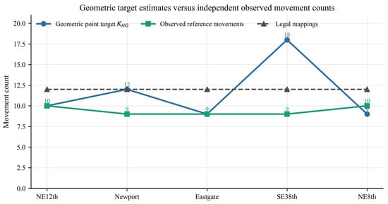
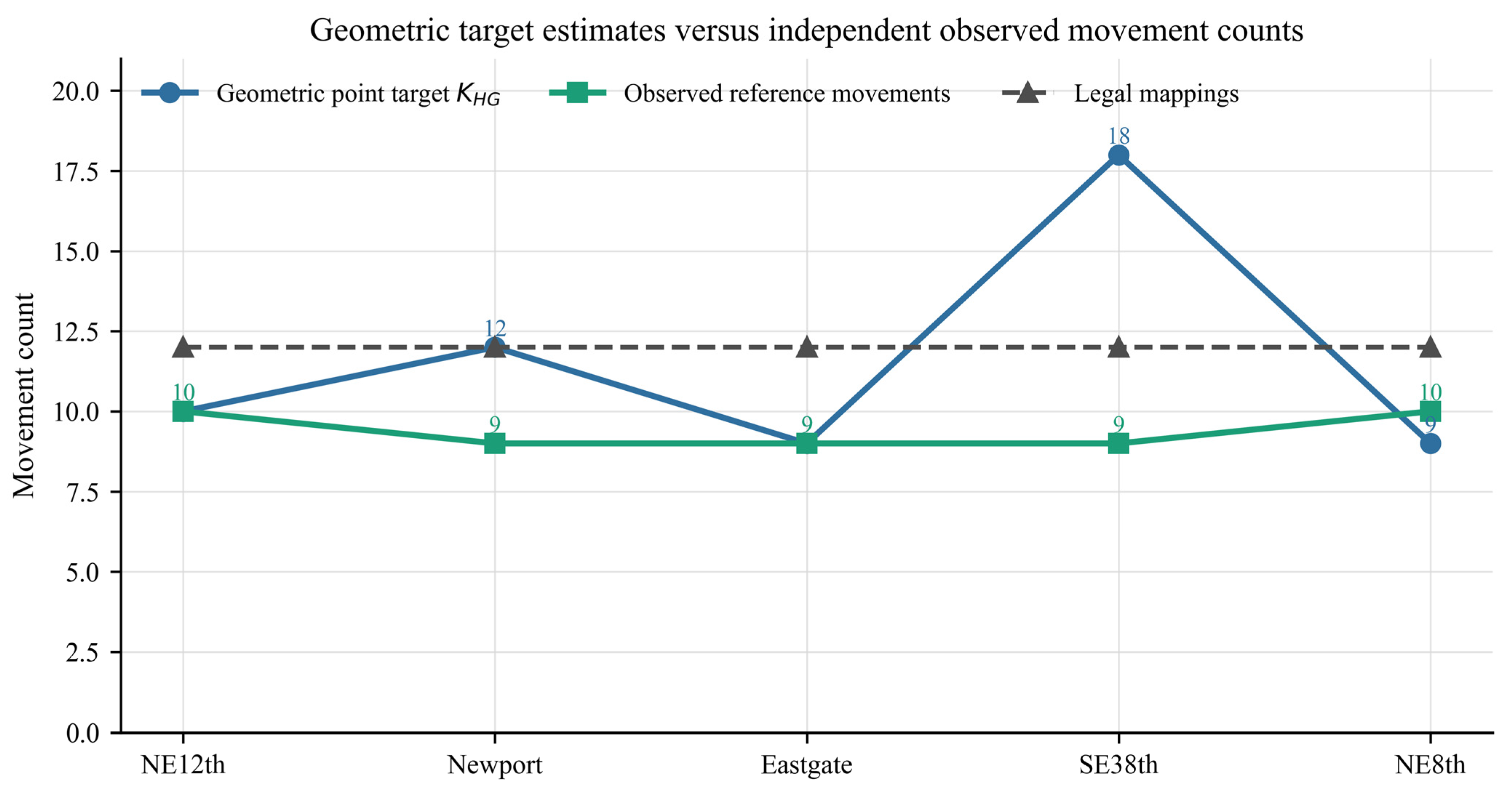
The independent rule-based reference contains 10, 9, 9, 9, and 10 observed movement classes in 116th/NE12th, Newport, Eastgate, SE38th, and NE8th, respectively. The corresponding geometric point targets $K_{\mathrm{H}\mathrm{G}}$ are 10, 12, 9, 18, and 9. Thus, the point estimator is exact in two scenes, differs by one movement in NE8th, and overestimates Newport by three and SE38th by nine. The mean scene-level absolute point-target error is 2.60 movements. Figure 4 contrasts the geometric point targets with independent observed and legal movement counts.

Figure 4. Geometric point-target estimates compared with independent observed movement counts and the twelve legal polygon-rule mappings defined for each scene. The SE38th point target is a visible over-segmentation failure rather than a corrected or excluded case.

SAC leaves the four-by-four endpoint structure unchanged in 116th/NE12th, Eastgate, and NE8th, consolidates Newport entry micro-modes from four to three supernodes, and reduces SE38th from seven to five entry regions and from three to two exit regions. The deterministic $K_{\mathrm{S}\mathrm{M}\mathrm{G}}$ values are 10, 8, 9, 10, and 9. Recording-aware bootstrap intervals are intentionally wider than single point targets, most notably [8,20] for SE38th, where endpoint geometry is intrinsically multimodal. The consolidation results and bootstrap target intervals are summarized in Table 4.

Table 4. From geometric micro-modes to semantic maneuver priors.

Scene	${\mathit{K}}_{\mathbf{H}\mathbf{G}}$	Entry Groups (Before → After)	Exit Groups (Before → After)	${\mathit{K}}_{\mathbf{S}\mathbf{M}\mathbf{G}}$	Bootstrap Target Interval 90%	Observed
116th/NE12th	10	4→4	4→4	10	[8,13]	10
150th/Newport	12	4→3	4→4	8	[7,13]	9
150th/Eastgate	9	4→4	4→4	9	[7,11]	9
150th/SE38th	18	7→5	3→2	10	[8,20]	9
NE8th	9	4→4	4→4	9	[9,10]	10

3.2. Independent-Test Comparison

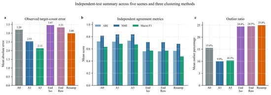
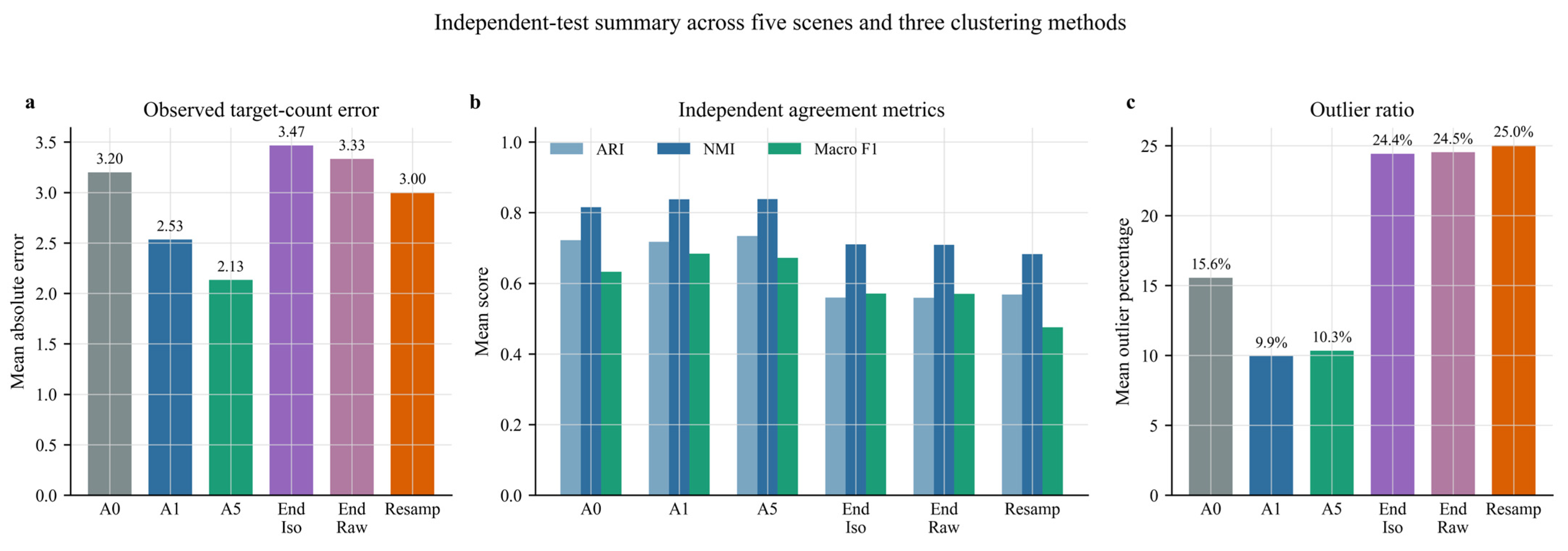
Table 5 summarizes the independent-test results averaged over the three clustering method families and five scenes. Among the primary methods and external baselines reported in Table 5, HG-SMG-TC achieves the lowest mean observed target-count error (2.13), the highest ARI (0.734), the highest NMI (0.839), and the highest weighted F1 (0.821). Relative to untargeted selection A0, HG-SMG-TC reduces target-count error from 3.20 to 2.13, lowers the outlier percentage from 15.56% to 10.34%, and improves NMI from 0.816 to 0.839 and macro F1 from 0.633 to 0.672.

Table 5. Aggregate independent-test comparison across five scenes and three clustering methods. ARI: adjusted Rand index; NMI: normalized mutual information.

Method	Target Err.	Outlier	ARI	NMI	Purity	Macro F1	Weighted F1
A0 untargeted	3.20	15.56%	0.722	0.816	0.910	0.633	0.790
A1 HG point-target	2.53	9.94%	0.718	0.838	0.934	0.684	0.817
HG-SMG-TC (A5)	2.13	10.34%	0.734	0.839	0.930	0.672	0.821
Endpoint raw	3.33	24.53%	0.559	0.709	0.832	0.570	0.688
Endpoint isotropic	3.47	24.43%	0.559	0.710	0.833	0.571	0.688
Resampled trajectory	3.00	25.02%	0.568	0.683	0.797	0.475	0.683

A5 further reduces target-count error from 2.53 to 2.13 and increases ARI from 0.718 to 0.734 and NMI from 0.838 to 0.839, but A1 has slightly higher purity (0.934 versus 0.930) and macro F1 (0.684 versus 0.672) and a slightly lower outlier percentage (9.94% versus 10.34%). Figure 5 provides a visual summary of the corresponding target-count, agreement, and outlier trade-offs.

Figure 5. Aggregate independent-test performance across five scenes and three clustering methods. (a) Mean absolute target-count error; lower values are better. (b) Mean adjusted Rand index (ARI), normalized mutual information (NMI), and macro F1 score; higher values are better. (c) Mean outlier percentage; lower values are better. A0: untargeted selection; A1: homography-guided point-target selection; A5: HG-SMG-TC; End Iso: isotropic endpoint baseline; End Raw: raw endpoint baseline; and Resamp: resampled-trajectory baseline.

3.3. Baseline Comparison and Scene-Level Paired Evidence

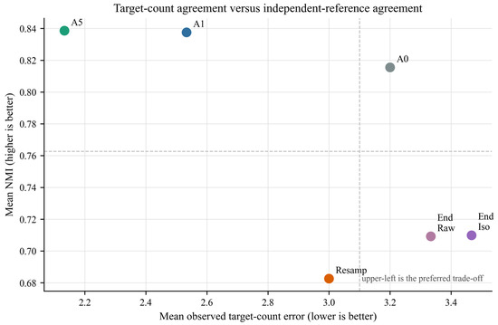
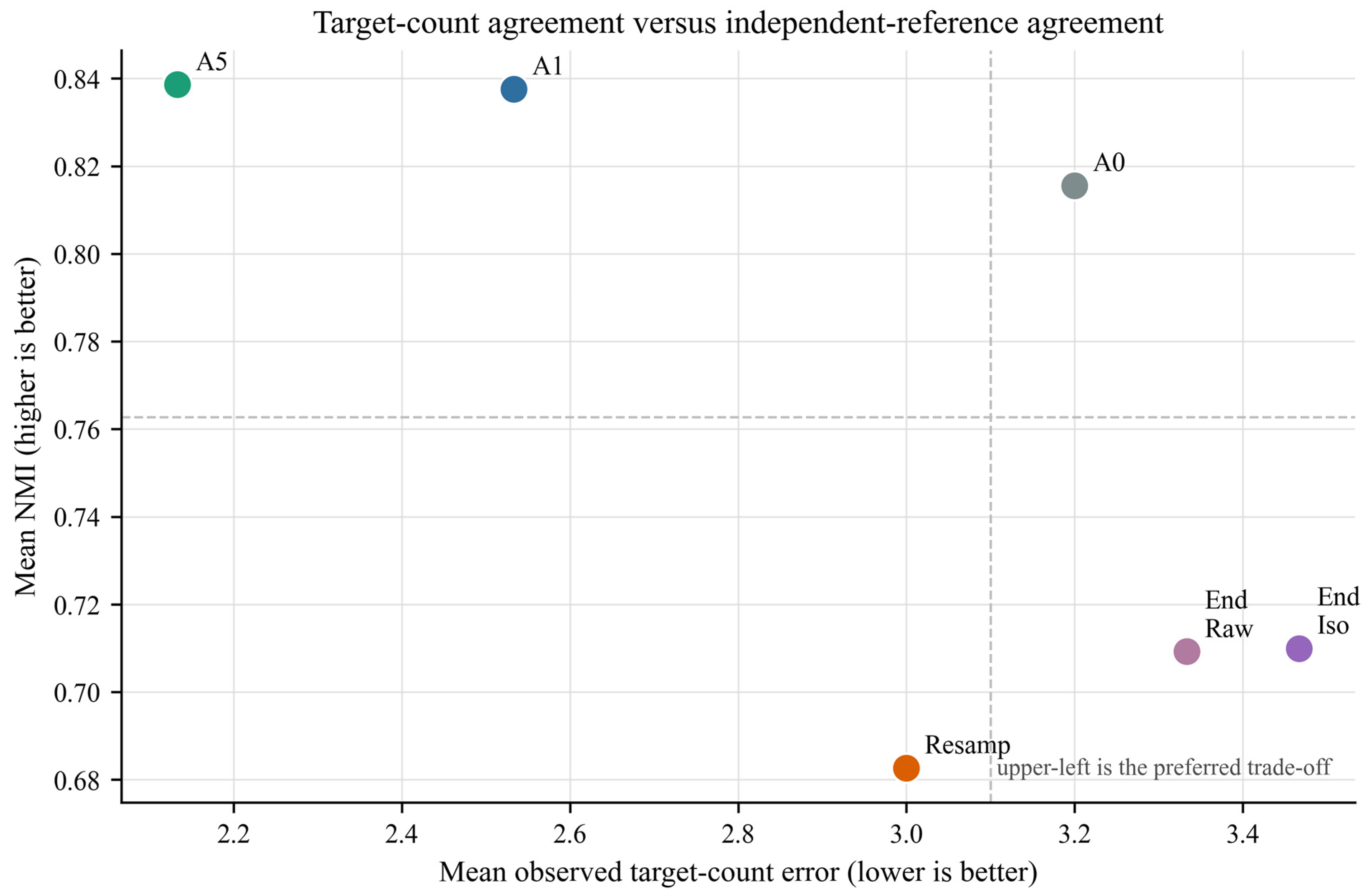
Endpoint information is a strong baseline because entry and exit locations already encode much of an intersection maneuver. Using aggregate macro F1 as the comparison criterion, the strongest endpoint baseline—the isotropically normalized endpoint representation—reaches mean NMI 0.710 and macro F1 0.571 with 24.43% outliers, compared with 0.839, 0.672, and 10.34% for HG-SMG-TC. The resampled full-trajectory baseline has lower NMI (0.683) and macro F1 (0.475), showing that simply adding trajectory shape does not guarantee better clustering. The trade-off between target-count alignment and independent-reference agreement is visualized in Figure 6.

Figure 6. Baseline comparison in the plane of mean observed target-count error and mean NMI. HG-SMG-TC combines lower target error with higher independent-reference agreement than the endpoint and resampled-trajectory baselines.

Scene-level paired summaries further separate the effect of repeated methods from the number of independent scenes. Relative to the strongest endpoint baseline, HG-SMG-TC has a mean target-error difference of −1.3333 movements and mean improvements of +0.129 NMI, +0.175 ARI, and +0.101 macro F1, while reducing outliers by 14.09 percentage points. The fixed-seed 95% bootstrap intervals over the five scene-level differences are shown in Table 6. Because n = 5 scenes, these intervals are reported descriptively and should not be interpreted as high-powered population-level inference.

Table 6. Paired scene-level differences: HG-SMG-TC minus the strongest endpoint baseline.

Metric	Mean Δ	Median Δ	95% Bootstrap Interval	Preferred Sign
Observed target error	−1.33	−1.33	[−2.20, −0.40]	negative
NMI	+0.129	+0.175	[+0.056, +0.187]	positive
ARI	+0.175	+0.198	[+0.074, +0.258]	positive
Macro F1	+0.101	+0.122	[+0.046, +0.145]	positive
Outlier percentage	−14.09 pp	−19.02 pp	[−19.80, −6.89] pp	negative

3.4. SE38th: Geometric Micro-Mode Over-Segmentation and Semantic Consolidation

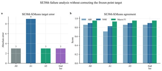
SE38th exposes the central failure mode that motivates semantic consolidation. EMD selects seven entry and three exit micro-regions and produces $K_{\mathrm{H}\mathrm{G}}$ = 18, whereas the independent rule-based reference contains nine observed semantic movements. Diagnostic mapping shows that four automatic entry regions are dominated by the same physical approach, eleven supported geometric OD pairs duplicate the dominant semantic movement of another pair, and eight pairs contain mixed semantic labels. Varying the support threshold alone cannot recover the semantic count: across the predefined threshold grid the point target remains between 14 and 19.

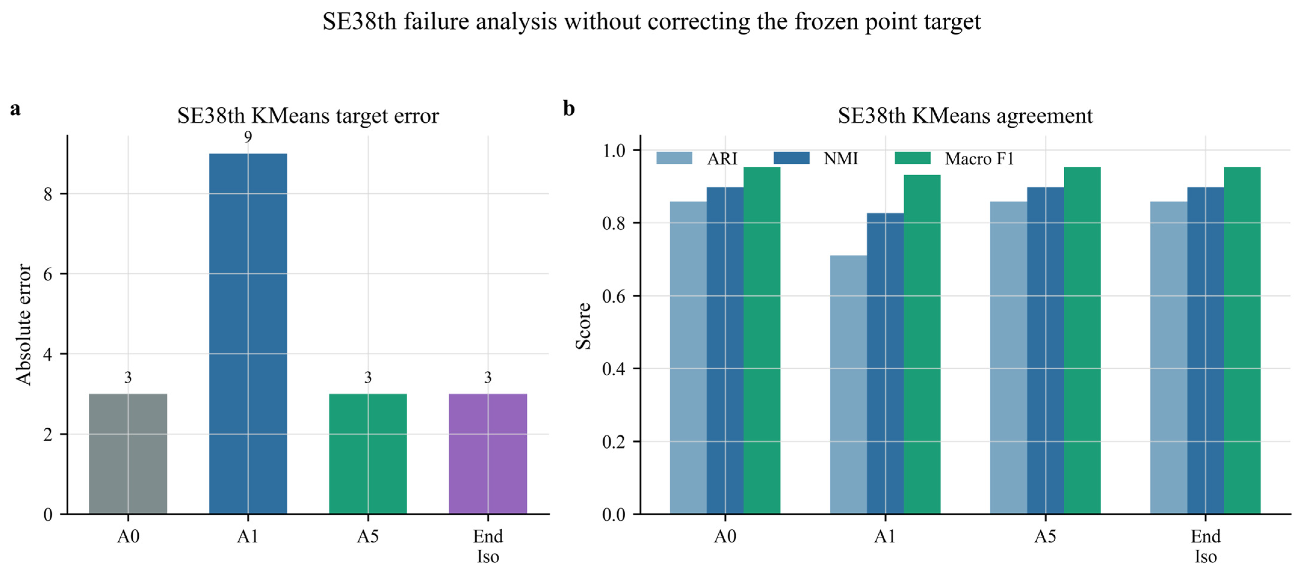
For KMeans, A1 therefore selects 18 clusters against nine observed movements. HG-SMG-TC consolidates the endpoint structure to five entry and two exit supernodes, gives deterministic $K_{\mathrm{S}\mathrm{M}\mathrm{G}}$ = 10 with a 90% target interval [8,20], and no longer forces KMeans to the geometric point target. Interval-constrained model selection selects 12 clusters. NMI increases from 0.827 to 0.898, ARI from 0.711 to 0.859, macro F1 from 0.932 to 0.953, and the mean effective number of clusters per movement decreases from 1.456 to 1.217. Figure 7 summarizes the change.

Figure 7. SE38th failure analysis. (a) KMeans observed target-count error for A0, A1, A5, and the isotropic endpoint baseline (End Iso); (b) KMeans ARI, NMI, and macro F1 for the same variants. Semantic consolidation relaxes the erroneous 18-cluster geometric point target, substantially reducing KMeans target-count error and fragmentation while increasing mapped agreement. A strong endpoint baseline remains competitive in this scene, confirming that endpoint geometry itself is highly informative.

The SE38th result also prevents an overly broad interpretation of HG-SMG-TC. Endpoint KMeans is itself strong in this scene and reaches comparable mapped agreement when it selects a similar cluster count. The contribution of HG-SMG-TC is therefore not that complex trajectory features universally outperform endpoints; it is that the scene-derived prior is constructed at a semantic-approach level and its uncertainty is propagated into model selection instead of enforcing raw geometric micro-mode counts.

3.5. Homography Quality and Sensitivity

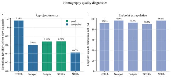
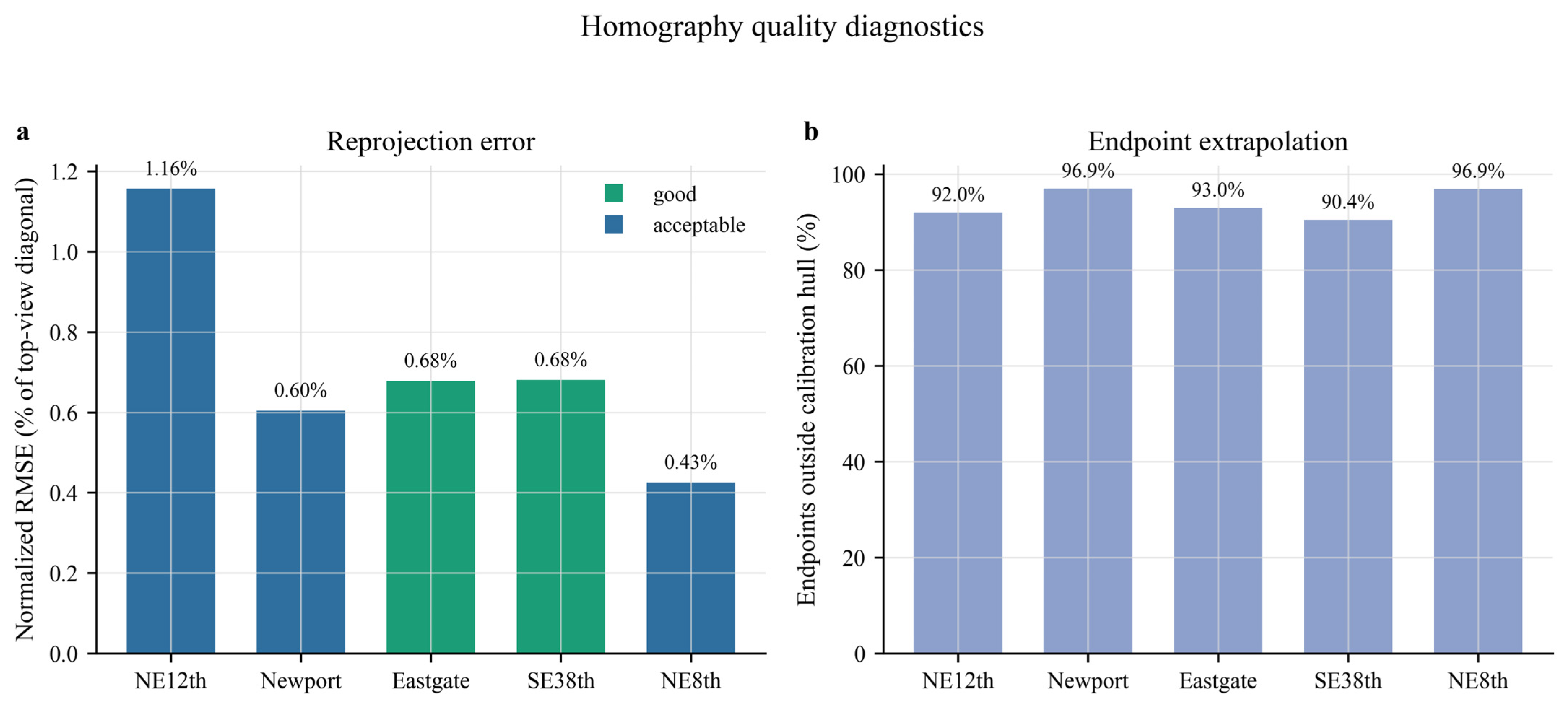
All five homographies are reproduced exactly from the calibration correspondence tables and pass the diagnostic engineering screening. Mean forward reprojection error ranges from 8.32 to 13.99 pixels and normalized RMSE from 0.43% to 1.16%. However, 90.43–96.95% of target-estimation endpoints lie outside the source control-point convex hull. These values justify using homography as a relative scene-structure layer but do not support claims of uniform metric spatial accuracy. Figure 8 summarizes the normalized reprojection error and endpoint extrapolation across the five scenes.

Figure 8. Homography quality and extrapolation diagnostics. (a) Normalized forward-reprojection RMSE for the five scenes, with colors indicating the diagnostic screening class; (b) percentage of target-estimation endpoints outside the source control-point convex hull. Reprojection RMSE is moderate relative to image scale, while endpoint extrapolation is high in every scene and is explicitly treated as a limitation.

Calibration sensitivity was evaluated in two ways. First, each of the 101 control-point correspondences was omitted once and the homography was recalculated, allowing us to measure the influence of individual calibration points. Second, 500 bounded random perturbations of the source control points were evaluated. SE38th retains $K_{\mathrm{H}\mathrm{G}}$ = 18 in every perturbation replicate through ±5 pixels. At ±10 pixels, 14 of 20 replicates remain at 18 and the target ranges from 16 to 37; none approach the independent semantic count of nine. Omitting individual control points 5 or 6 can raise the target to 43, revealing local fragility, but the absence of any small-perturbation path toward nine indicates that SE38th over-segmentation is primarily a representational problem in endpoint-region granularity rather than a simple calibration-noise artifact.

3.6. Diagnostic-Score and Component Sensitivity

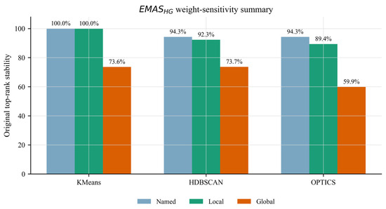
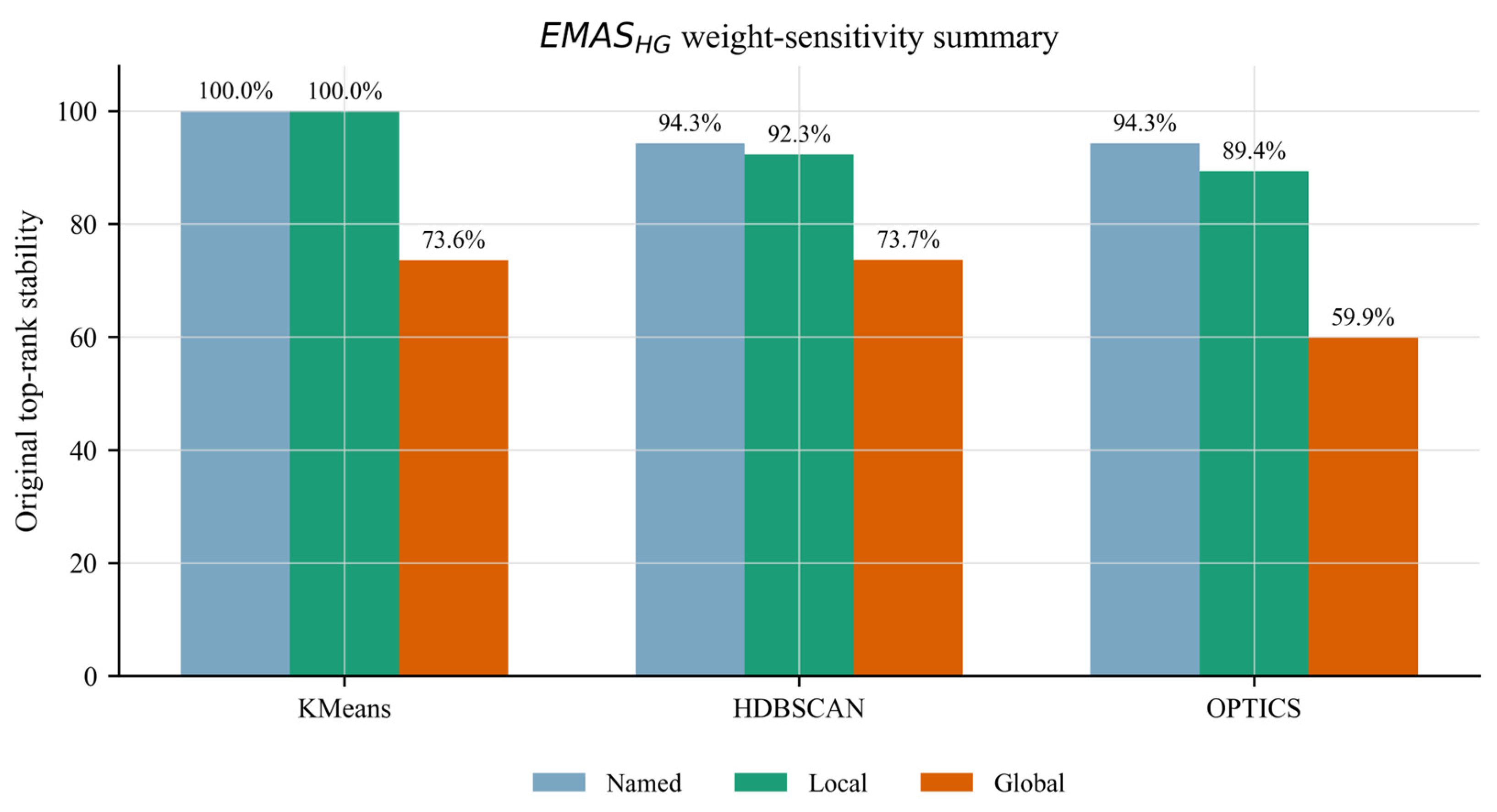
Because EMAS_HG-v1 uses heuristic component weights, we also tested whether moderate changes in these weights would alter the selected configurations. The canonical implementation reproduces the released diagnostic outputs to numerical precision. Replacing the primary weights with $0.40T+0.30O+0.10B+0.10S+0.10D$ preserves the top model-selection candidate in 14 of 15 scene–method groups. Across a 465-vector local weight grid, the primary top rank is preserved in 93.88% of cases, with mean Spearman and Kendall correlations of 0.967 and 0.920, respectively. The score is therefore locally stable in most groups but remains a heuristic diagnostic rather than independent evidence. Figure 9 summarizes the weight-sensitivity results by clustering method family.

Figure 9. Local weight sensitivity of the Expected-Maneuver Alignment Score computed with the homography-guided target (EMAS_HG) by clustering method family. The percentage above each bar denotes preservation of the original top-ranked candidate under the tested alternative weights. High but incomplete stability supports the use of the score as a diagnostic rather than as a universal clustering-validity index.

Component ablations also clarify the new method. Point-target semantic variants A2/A3/A10 achieve tighter mean target error (1.80) and slightly higher mean NMI (0.851) than A5, but they collapse the estimated target distribution back to a single count. Bearing-only SAC (A6) matches A5 on the aggregate metrics, while heading-only SAC (A7) deteriorates sharply to target error 4.40, NMI 0.754, and macro F1 0.383. Top-view heading (A9) matches the primary camera-isotropic heading variant. These results indicate that side/bearing structure is essential in the tested scenes, while local heading contributes less strongly and the interval prior represents a robustness choice rather than an optimization for every mean metric. Selected component ablations are summarized in Table 7.

Table 7. Selected independent-test ablations of the HG-SMG-TC components.

Variant	Target Err.	NMI	ARI	Macro F1	Outlier
A0 untargeted	3.20	0.816	0.722	0.633	15.56%
A1 point target	2.53	0.838	0.718	0.684	9.94%
A2/A3/A10 point-target semantic variants	1.80	0.851	0.747	0.668	10.00%
A5 full HG-SMG-TC	2.13	0.839	0.734	0.672	10.34%
A6 bearing-only SAC	2.13	0.839	0.734	0.672	10.34%
A7 heading-only SAC	4.40	0.754	0.630	0.383	15.23%
A9 top-view heading	2.13	0.839	0.734	0.672	10.34%

4. Discussion

4.1. Main Finding and Methodological Novelty

The main result is that target-aware trajectory clustering becomes more defensible when the scene-derived target is treated as an uncertain semantic prior rather than as an exact count of geometric endpoint pairs. HG-SMG-TC is a new model-selection method built around this distinction. It does not introduce a new base clustering algorithm; instead, it changes how scene structure is represented and how that structure constrains KMeans, HDBSCAN, and OPTICS. This distinction is important because the largest failure in the point-target formulation, SE38th, is caused by geometric micro-modes that are real in the endpoint distribution but do not correspond one-to-one with semantic traffic movements.

The literature comparison supports novelty at the level of the complete coupled formulation. Endpoint-region discovery and OD counting [18,19], lane/geometric-mode extraction and trajectory graphs [20,21,22,23,24], and multi-criteria cluster ranking [25] each have clear prior art. The present method combines these ideas in a different role: homography-derived endpoint modes are intermediate geometric objects; label-free directional consolidation creates approach-level supernodes; the semantic maneuver graph aggregates micro-OD support; recording-aware bootstrap converts the graph into a target interval; and interval distance enters an unsupervised model-selection key whose final evaluation is isolated from the reference labels. No work identified in the reviewed literature combines all of these stages for fixed-camera trajectory clustering.

4.2. Target Alignment, Independent Agreement, and Internal Compactness

The independent-test results reject a single-metric interpretation. HG-SMG-TC improves mean target-count alignment, ARI, NMI, and weighted F1 relative to A0, and substantially outperforms the endpoint and resampled-trajectory baselines in aggregate. At the same time, A1 retains slightly better purity, macro F1, and outlier rate than A5. This is not a contradiction: cluster-count alignment, semantic class agreement, internal compactness, and noise rejection measure different properties. The point-target logic can generate compact or pure partitions in some scenes while still being semantically over-constrained in others.

For this reason, EMAS_HG is deliberately separated from independent validation. Its target-count term is structurally related to the target-aware design, and its components are correlated. The primary validity evidence in this paper is instead the label-isolated reference evaluation, together with scene-level paired baseline comparisons and transparent failure analysis. This also explains why the proposed method is not selected retrospectively from the best independent-test mean among the ablations: the full A5 formulation is the uncertainty-aware method pre-specified before independent-test evaluation, whereas A2/A3/A10 collapse the target distribution to a single point.

4.3. Endpoint Information, Baselines, and the Role of the Semantic Graph

The strong endpoint baselines are scientifically informative rather than inconvenient. Intersection maneuvers are heavily determined by where trajectories enter and leave the observed scene, so an endpoint-only KMeans baseline can be competitive, especially at SE38th. The resampled full-trajectory baseline performs worse in aggregate, showing that added trajectory shape can introduce within-maneuver variation without necessarily adding discriminative structure. HG-SMG-TC therefore should not be interpreted as evidence that richer trajectory features are always superior. Its benefit lies in converting readily available endpoint geometry into a structured, uncertainty-aware prior that can guide several clustering families.

The semantic graph is also deliberately simpler than lane-network reconstruction. SAC does not attempt to infer lane centerlines, map topology, or legal traffic rules. The graph summarizes supported relations between consolidated approach-level supernodes. This narrower representation reduces the risk of claiming information that cannot be supported by sparse manual homography calibration, while still solving the model-selection problem exposed by geometric micro-mode duplication.

4.4. Calibration and Reproducibility Implications

Homography remains useful despite high endpoint extrapolation because it is not used as a metric ground-truth coordinate system. The camera-to-top-view transform provides relative angular and side information for endpoint organization; final clustering remains in isotropically normalized camera coordinates. The perturbation study further shows that the SE38th semantic discrepancy is not removed by plausible small control-point noise. Consequently, the principal methodological limitation of the point target is not simply homography accuracy but the representational assumption that every supported endpoint mode corresponds to a distinct maneuver.

The workflow is reproducible at the numerical level. Target-estimation and selection protocols, calibration correspondences and inlier masks, homography matrices, candidate grids, seeds, reference polygons and mappings, assignment manifests, compact results, and figure sources are published with the project materials. The design also makes manual input explicit: calibration still requires point correspondences and the independent reference requires human-defined polygons and legal OD mappings. These inputs are not hidden inside automatic tuning.

4.5. Limitations

Several limitations bound the conclusions. First, the study covers five Bellevue intersections from one dataset, so the results establish multi-scene evidence rather than broad geographic generalization. Second, the polygon-rule reference is exhaustive and independent of clustering outputs but is not a trajectory-by-trajectory dual-annotator ground truth; boundary sensitivity and unassignable cases are reported instead of inter-rater agreement. Third, homography uses manually selected correspondences, no lens-distortion correction, and sparse calibration hulls with high endpoint extrapolation. Fourth, $K_{\mathrm{S}\mathrm{M}\mathrm{G}}$ remains a heuristic estimate of supported observed maneuver structure rather than a legal-movement inventory, and the SE38th bootstrap interval remains broad. Fifth, full pairwise DTW and Fréchet baselines are computationally infeasible at the complete independent-test scale and are not reported. Finally, the scene-level statistical sample is only five, so uncertainty intervals should be interpreted descriptively. Evaluation on prospectively collected intersections, independently annotated maneuver references, and topology-aware consolidation would provide the strongest next test of generalization.

5. Conclusions

This paper presented HG-SMG-TC, a method for using simple geometric information from a traffic camera to guide unsupervised vehicle-trajectory clustering. The starting point is a practical problem: endpoint clustering may identify several geometric groups for vehicles that, from a traffic perspective, belong to the same road approach. Treating every such group as a separate maneuver can therefore lead to an unrealistically high expected cluster count. HG-SMG-TC addresses this problem by consolidating compatible endpoint groups into approach-level groups, constructing a maneuver graph from the observed origin-destination relations, and estimating a range of plausible maneuver counts by bootstrap resampling. This range is then used during clustering model selection rather than forcing the solution toward one fixed target.

The evaluation uses separate recording-block splits for prior estimation, model selection, and independent testing, with assignments persisted before the human-defined polygon-rule reference is read. Across five Bellevue scenes and three clustering families, the proposed method achieves the best mean target-count error, ARI, NMI, and weighted F1 among the primary methods and reported baselines, while retaining an explicit trade-off against the slightly higher macro F1 and purity of the point-target A1 variant. Relative to the strongest endpoint baseline, HG-SMG-TC improves aggregate NMI and macro F1 while reducing outliers by approximately fourteen percentage points. The SE38th analysis provides the clearest mechanism-level evidence: semantic consolidation prevents an 18-mode geometric endpoint structure from being enforced as an 18-cluster semantic solution and substantially improves independent-reference agreement.

The contribution is therefore not a claim of universally superior clustering. It is a new and reproducible way to connect lightweight scene geometry to unsupervised model selection while propagating uncertainty and keeping evaluation labels isolated from the method. This formulation makes target-aware search more suitable for heterogeneous fixed-camera intersections where geometric substructure and semantic traffic movements do not coincide exactly.

References

- Yu, F.; Ao, W.; Yan, H.; Zhang, G.; Wu, W.; Li, Y. Spatio-temporal vehicle trajectory recovery on road network based on traffic camera video data. In Proceedings of the 28th ACM SIGKDD Conference on Knowledge Discovery and Data Mining, Washington, DC, USA, 14–18 August 2022; pp. 4413–4421. [Google Scholar] [CrossRef] [Scilit]
- Yu, F.; Yan, H.; Chen, R.; Zhang, G.; Liu, Y.; Chen, M.; Li, Y. City-scale vehicle trajectory data from traffic camera videos. Sci. Data 2023, 10, 711. [Google Scholar] [CrossRef] [Scilit]
- Wu, D.; Fang, Z.; Sun, Q.; Chen, L.; Hu, H.; Wang, F.; Gao, Y. TrajRecovery: An efficient vehicle trajectory recovery framework based on urban-scale traffic camera records. In Proceedings of the 30th ACM SIGKDD Conference on Knowledge Discovery and Data Mining, Barcelona, Spain, 25–29 August 2024; pp. 5979–5990. [Google Scholar] [CrossRef] [Scilit]
- Li, Z.; Li, Z.; Hu, X.; Du, G.; Nie, Y.; Zhu, F.; Bai, L.; Zhao, R.; Lv, Y. VisionTraj: A noise-robust trajectory recovery framework based on large-scale camera network. IEEE Trans. Intell. Transp. Syst. 2025, 26, 15826–15837. [Google Scholar] [CrossRef] [Scilit]
- Abdel-Aty, M.; Wang, Z.; Zheng, O.; Abdelraouf, A. Advances and applications of computer vision techniques in vehicle trajectory generation and surrogate traffic safety indicators. Accid. Anal. Prev. 2023, 191, 107191. [Google Scholar] [CrossRef] [Scilit]
- Zhang, L.; Yu, X.; Daud, A.; Mussah, A.R.; Adu-Gyamfi, Y. Application of 2D homography for high resolution traffic data collection using CCTV cameras. arXiv 2024, arXiv:2401.07220. [Google Scholar]
- Agg, Á.D.; Péter, B.G.; Horváth, A. Traffic Node Video Dataset: For modelling the trajectories of moving objects in traffic based on visual analysis. In Proceedings of the Spring Wind, Budapest, Hungary, 3–5 May 2024; pp. 183–197. [Google Scholar]
- Agg, Á.D.; Péter, B.G.; Horváth, A. Automata forgalmi statisztika objektumdetektálás és adaptív járműtrajektória klaszterezés alapján. Közlek. Mobilitás 2023, 2023, 36. [Google Scholar] [CrossRef] [Scilit]
- Agg, Á.D.; Péter, B.G.; Horváth, A. Adaptive vehicle trajectory clustering based on computer vision. In Cognitive Mobility; Zöldy, M., Ed.; Lecture Notes in Networks and Systems; Springer: Cham, Switzerland, 2025; Volume 1258, pp. 344–360. [Google Scholar] [CrossRef] [Scilit]
- Campos Ruiz, R.E.; Petraglia, M.R.; Boscher Torres, J.C. Automated traffic camera calibration via panoramic image-based 3D scene reconstruction. Meas. Sci. Technol. 2025, 36, 096301. [Google Scholar] [CrossRef] [Scilit]
- Song, J.-F.; Fan, Y.; Song, H.; Zhao, H. Target tracking and 3D trajectory reconstruction based on multicamera calibration. J. Adv. Transp. 2022, 2022, 5006347. [Google Scholar] [CrossRef] [Scilit]
- Wang, W.; Xia, F.; Nie, H.; Chen, Z.; Gong, Z.; Kong, X.; Wei, W. Vehicle trajectory clustering based on dynamic representation learning of Internet of Vehicles. IEEE Trans. Intell. Transp. Syst. 2020, 22, 3567–3576. [Google Scholar] [CrossRef] [Scilit]
- Chen, B.; Luo, Y.; Zhang, Y.; Jia, T.; Chen, H.-P.; Gong, J.; Li, Q. Efficient and scalable DBSCAN framework for clustering continuous trajectories in road networks. Int. J. Geogr. Inf. Sci. 2023, 37, 1693–1727. [Google Scholar] [CrossRef] [Scilit]
- Cleju, N.; Catargiu, C. Extracting vehicle trajectory clusters from video monitoring in smart intersections. In Proceedings of the 2025 IEEE International Black Sea Conference on Communications and Networking (BlackSeaCom); IEEE: Piscataway, NJ, USA, 2025; pp. 1–6. [Google Scholar] [CrossRef] [Scilit]
- Rezaie, M.; Saunier, N. Trajectory clustering performance evaluation: If we know the answer, it is not clustering. arXiv 2021, arXiv:2112.01570. [Google Scholar]
- Rousseeuw, P.J. Silhouettes: A graphical aid to the interpretation and validation of cluster analysis. J. Comput. Appl. Math. 1987, 20, 53–65. [Google Scholar] [CrossRef] [Scilit]
- Davies, D.L.; Bouldin, D.W. A cluster separation measure. IEEE Trans. Pattern Anal. Mach. Intell. 1979, PAMI-1, 224–227. [Google Scholar] [CrossRef] [Scilit]
- Rathore, P.S.; Pattanaik, V.; Rathore, P. Unsupervised detection of entry and exit regions from vehicle trajectories for camera-agnostic turning movement counts. arXiv 2026, arXiv:2607.10949. [Google Scholar]
- Betru, A.; Tran, T.; Ectors, W. Automating composition of origin-destination flows of intersections based on UAV data. Procedia Comput. Sci. 2025, 257, 233–240. [Google Scholar] [CrossRef] [Scilit]
- Uduwaragoda, E.R.I.A.C.; Perera, A.S.; Dias, S.A.D. Generating lane level road data from vehicle trajectories using kernel density estimation. In Proceedings of the 2013 16th International IEEE Conference on Intelligent Transportation Systems (ITSC), The Hague, The Netherlands, 6–9 October 2013; pp. 384–391. [Google Scholar] [CrossRef] [Scilit]
- Wang, J.; Wang, C.; Song, X.; Raghavan, V. Automatic intersection and traffic rule detection by mining motor-vehicle GPS trajectories. Comput. Environ. Urban Syst. 2017, 64, 19–29. [Google Scholar] [CrossRef] [Scilit]
- Yuan, M.; Yue, P.; Yang, C.; Li, J.; Yan, K.; Cai, C.; Wan, C. Generating lane-level road networks from high-precision trajectory data with lane-changing behavior analysis. Int. J. Geogr. Inf. Sci. 2024, 38, 243–273. [Google Scholar] [CrossRef] [Scilit]
- Wan, C.; Yue, P.; Yang, C.; Cai, C.; Liu, X. Lane extraction from trajectories at road intersections based on Graph Transformer Network. Int. J. Geogr. Inf. Sci. 2025, 39, 758–787. [Google Scholar] [CrossRef] [Scilit]
- Du, J.; Liu, X.; Meng, C. Road intersection extraction based on low-frequency vehicle trajectory data. Sustainability 2023, 15, 14299. [Google Scholar] [CrossRef] [Scilit]
- Sekh, A.A.; Dogra, D.P.; Kar, S.; Roy, P.P. Video trajectory analysis using unsupervised clustering and multi-criteria ranking. Soft Comput. 2020, 24, 16643–16654. [Google Scholar] [CrossRef] [Scilit]
- Hartley, R.; Zisserman, A. Multiple View Geometry in Computer Vision, 2nd ed.; Cambridge University Press: Cambridge, UK, 2004. [Google Scholar]
- Fischler, M.A.; Bolles, R.C. Random sample consensus: A paradigm for model fitting with applications to image analysis and automated cartography. Commun. ACM 1981, 24, 381–395. [Google Scholar] [CrossRef] [Scilit]
- MacQueen, J. Some methods for classification and analysis of multivariate observations. In Proceedings of the Fifth Berkeley Symposium on Mathematical Statistics and Probability; University of California Press: Berkeley, CA, USA, 1967; Volume 1, pp. 281–297. [Google Scholar]
- Campello, R.J.G.B.; Moulavi, D.; Sander, J. Density-based clustering based on hierarchical density estimates. In Advances in Knowledge Discovery and Data Mining; Springer: Berlin/Heidelberg, Germany, 2013; pp. 160–172. [Google Scholar] [CrossRef] [Scilit]
- Ankerst, M.; Breunig, M.M.; Kriegel, H.-P.; Sander, J. OPTICS: Ordering points to identify the clustering structure. In Proceedings of the ACM SIGMOD International Conference on Management of Data, Philadelphia, PA, USA, 1–3 June 1999; pp. 49–60. [Google Scholar] [CrossRef] [Scilit]
Disclaimer/Publisher’s Note: The statements, opinions and data contained in all publications are solely those of the individual author(s) and contributor(s) and not of MDPI and/or the editor(s). MDPI and/or the editor(s) disclaim responsibility for any injury to people or property resulting from any ideas, methods, instructions or products referred to in the content. |
© 2026 by the authors. Licensee MDPI, Basel, Switzerland. This article is an open access article distributed under the terms and conditions of the Creative Commons Attribution (CC BY) license.