


Abstract
The emergence of unmanned aerial vehicles (UAVs) introduces new opportunities for the design of intelligent and flexible transportation systems beyond traditional road-based logistics. This study investigates the integration of UAVs as an alternative transportation mode within industrial environments, focusing on the rapid delivery of critical spare parts in large-scale production facilities. A two-stage optimization framework is developed, combining demand pre-processing with a routing algorithm that determines fleet utilization and delivery schedules under operational constraints. The proposed framework utilizes a data pre-processing stage, which converts enterprise resource planning order records into delivery-ready item data, with a mixed-integer linear programming (MILP) routing model that assigns eligible spare parts to UAV trips and determines the use of a fixed fleet under payload, dimensional, service-time, and battery-related constraints. The approach is evaluated using real annual order data from a metal-industry plant, combined with simulated intra-day arrival profiles due to the absence of exact order-placement timestamps in the ERP records. The results indicate that UAV-based transportation can serve a substantial share of internal demand while achieving shorter delivery-response times for the modeled UAV layer under the simulated dispatch instances and significantly lower direct energy-related transportation costs compared with the existing pickup-based process. The results highlight the role of UAVs as a complementary transportation layer in controlled industrial networks, supporting the transition toward more responsive and intelligent future transportation systems.
1. Introduction
Internal transportation is a critical component of industrial logistics because it determines how quickly materials, spare parts, tools, and operational information move within a production facility. In capital-intensive metal and aluminum production environments, maintenance workshops are dispersed over an extensive but bounded industrial area, while spare-parts inventory is usually concentrated in a central warehouse. This centralization improves control and inventory cost management, but it also creates recurrent internal transport movements between the warehouse and maintenance locations. When spare parts are needed during production disruptions, the elapsed delivery time can influence mean time to repair (MTTR) and overall equipment effectiveness (OEE).
The purpose of the study is to examine the feasibility and usefulness of introducing a UAV-based distribution model for maintenance spare parts in a large industrial unit in the metals sector. The paper formulates four research questions: (i) What was the delivery workload handled by the warehouse during the reference period, and what proportion of this workload could be covered by the proposed system? (ii) How can an efficient routing algorithm be designed and implemented to support the proposed delivery system? (iii) What operational parameters are required for the implementation of the proposed delivery system, including fleet structure, payload-basket dimensions, and landing-zone requirements? and (iv) How does the proposed UAV delivery system perform, and how do its results translate into operational cost savings?
The existing transport mode relies on pickup-type internal-combustion vehicles, usually involving a driver and an accompanying carrier, and is therefore affected by worker availability, routing variability within the industrial site, and the cost of ground transport. Rather than replacing this system entirely, the proposed article frames UAVs as a complementary transportation layer for lightweight and dimensionally compatible spare parts. Accordingly, this article examines a real case-study dataset, develops a preprocessing algorithm and a MILP-based routing algorithm, and compares the cost performance of the current as-is process with that of the proposed to-be process. This positioning is important because the problem extends beyond warehouse automation and should instead be framed as a controlled network transport design problem where a new aerial mode is inserted into an existing industrial network with known nodes, operational constraints, and measurable demand.
The remainder of the article is structured as follows. Section 2 reviews the relevant literature and identifies the research gap. Section 3 presents the case-study setting, data-preprocessing procedure, and MILP routing formulation. Section 4 reports the computational and economic evaluation results. Section 5 discusses the implications, limitations, and future research directions, while Section 6 concludes the article.
2. Review and Research Gap
The routing problem underlying this study originates in classical vehicle-routing research. The Traveling Salesman Problem (TSP) and the Vehicle Routing Problem (VRP) established the basic structure of cost- or time-minimizing delivery tours, while exact optimization, integer programming, and heuristic approaches provided the early methodological base for practical routing [1,2,3]. The literature review indicates that modern UAV routing inherits these classical foundations but must adapt them to the characteristics of aerial vehicles, especially limited battery duration, payload limits, energy consumption, and the possibility of operating independently from, or in cooperation with, ground vehicles. As a result, UAV routing problems often combine routing, scheduling, and resource-feasibility decisions within a single optimization framework.
A first set of UAV logistics research articles studies hybrid truck-drone systems. The flying sidekick traveling salesman problem introduced the principle of parallel service, where a truck can launch a drone while continuing its own route [4]. Subsequent work extended this idea to multiple trips, multiple drones, time windows, energy-aware routing, and branch-and-price or constraint-programming formulations [5,6,7,8,9]. The main modeling challenge is therefore synchronization: the truck and drone must be coordinated so that waiting times, launch and recovery operations, and parallel service opportunities are jointly optimized. This structure is highly relevant for last-mile distribution, but it differs from the present industrial setting, where UAVs operate from a fixed warehouse depot and are not synchronized with a moving ground vehicle. The mentioned coupling is precisely what makes these models inapplicable to the present approach; removing the truck does not specialize a truck–drone model but dismantles its central decision structure.
A second set of articles studies drone-only delivery. Drone-only routing studies are closer to the present setting because they consider repeated UAV trips from fixed depots. Here, the central modeling challenges are the feasibility of repeated UAV trips from a depot, the effect of payload on speed or energy consumption, and the scheduling of multiple drones under battery and capacity restrictions. The review highlights models such as load-dependent flight-speed routing, multi-trip drone routing [10,11] and energy-function formulations [12,13,14,15,16,17]. These approaches are especially relevant to spare-parts intralogistics because the payload of an individual SKU can materially affect the feasible route and because several short flights from a fixed depot may be operationally preferable to a single heavier route. However, these models typically represent demand as an aggregate quantity at each customer node and assume that a customer is served by a single visit. In the spare-parts setting this representation is infeasible: a single workshop order is a heterogeneous bundle of distinct SKUs whose combined mass and volume frequently exceed the capacity of one trip, so the order must be divisible across several trips and several drones while individual pieces remain indivisible. A node-aggregated, single-visit formulation cannot express this piece-level splitting without being structurally rebuilt. Energy-budget formulations face a separate obstacle: they constrain each route against an energy allowance, whereas the operational requirement here is dispatch within a finite, interval-triggered horizon against a hard service-time deadline, and the nonlinear payload–energy terms common in this stream are difficult to solve within the sub-ten-minute window demanded by live warehouse operation.
A third stream of articles concerns industrial intralogistics. Practical examples identified in the literature review include industrial experiments in which drones transport spare parts or production components within manufacturing plants [18,19,20]. These examples support the physical feasibility of intra-plant UAV-based transport, but the review identifies that the academic literature has not yet treated factory-level, spare-parts delivery with the same depth as urban last-mile parcel delivery. They provide no routing or scheduling formulation that links enterprise demand to fleet-level decisions and therefore offer no optimization model that could be transferred to the present problem. Industrial networks differ from urban networks because they are geographically constrained, have stable delivery nodes, may operate under plant-specific safety rules, and are directly connected to maintenance response and production continuity. These characteristics make industrial UAV routing a distinct transportation-design problem rather than a direct transfer of urban drone-delivery models.
The research gap addressed in this article is the lack of a detailed, data-driven UAV routing framework for repeated spare-parts delivery within a controlled industrial intralogistics network. Existing studies provide strong foundations for truck-drone coordination and drone-only delivery, but the case-study setting requires a formulation that connects real ERP-based demand, workshop-level delivery nodes, strict item eligibility filters, and fleet-level routing decisions. The problem also differs from generic parcel delivery because the transportation task supports maintenance operations in a production plant, where service time and operational reliability are central concerns. Therefore, there is the need for a formulation in which the unit of demand is the indivisible spare-part piece rather than the node; demand can be split across a fixed multi-trip fleet under joint mass, volume, and dimensional eligibility constraints; payload effects on flight time are linearized for operational-speed solution; and dispatch is governed by a service-time deadline within a rolling order accumulation window. None of the cited models can be adapted to satisfy these requirements simultaneously without replacing their core decision structure.
To address this gap, this article makes four contributions to the literature on UAV-enabled transportation systems and industrial intralogistics. First, it reframes UAV delivery as a controlled network transport-design problem within a bounded industrial plant, rather than as a generic last-mile parcel-delivery problem. Second, it develops a data-preprocessing procedure that transforms ERP-based spare-parts order records into routing-ready demand instances, linking real industrial demand with UAV routing decisions. Third, it formulates a MILP routing model that assigns indivisible spare-parts pieces to UAV trips, selects routes for a fixed UAV fleet, accounts for payload and service constraints, and minimizes total UAV operating time. Fourth, it evaluates the framework on real case-study demand data, reporting demand coverage, solver performance, fleet-utilization patterns, route examples, and a screening-level direct energy-cost comparison with the existing pickup-based process. Through these contributions, the article focuses on a descriptive assessment of UAV industrial delivery feasibility and lays the foundation toward an optimization-based evaluation of how an aerial transport layer can be integrated into an existing real-world industrial maintenance-logistics network.
The novelty of the routing model is not observed in any specific single mechanism but rather in the specific composition required by the operational constraints and in one structural departure from the drone-only literature. Whereas standard multi-trip drone-routing models treat demand as an aggregate quantity attached to a customer node, the present formulation defines demand at the level of the indivisible piece: each order line is a unit p with its own mass and volume, pieces are assigned to trips rather than nodes, and a single workshop may consequently be served across several trips and several drones. This piece-level assignment is the feature that node-aggregated formulations cannot reproduce, and it is what allows real ERP order bundles, mixtures of many heterogeneous SKUs, to be routed feasibly. Around this core, the model integrates, within a single MILP solvable at operational speed, a fixed multi-trip fleet with per-UAV chronological trip sequencing, joint mass and volume capacities with upstream dimensional eligibility, a piecewise-linear coupling of arc travel time to carried load via the arc commodity flow, and a deadline-oriented operating horizon. It is the simultaneous presence of these elements, rather than any one of them, that distinguishes the formulation from prior multi-trip drone-only models.
3. Materials and Methods
This section describes the methodological framework developed to assess the feasibility and operational performance of the proposed UAV-based spare-parts delivery system. The framework combines a real industrial case-study dataset, UAV eligibility rules, operational assumptions, data preprocessing, and a MILP routing model. The section first presents the case study setting and demand data, then specifies the flight eligibility criteria and operating assumptions, before detailing the optimization model and the evaluation scenario used for computational and cost analysis.
3.1. Case-Study Description
The setting of this case study consists of one central spare-parts warehouse and seventeen maintenance workshops. The warehouse is treated as the depot node and the workshops as customer nodes. The graph model is constructed from the workshops’ and warehouse’s coordinates, and Euclidean distances are used between nodes when the distance matrix for the routing model is created. This assumption is adopted to support the feasibility-stage evaluation of UAV-based spare-parts distribution and to keep the MILP focused on fleet assignment, payload feasibility, route sequencing, and operating-time minimization. Similar Euclidean-distance representations are frequently used in UAV-routing formulations when the objective is to evaluate routing performance rather than to design certified low-level trajectories [13,21,22]. Nevertheless, Euclidean distance may underestimate the feasible flight distance in an industrial plant. In practice, UAVs may need to follow approved safety corridors, avoid production equipment and no-fly zones, comply with altitude restrictions, and satisfy plant-specific safety rules. Therefore, a detour coefficient was introduced as a conservative adjustment to the Euclidean travel-time matrix, corresponding to a 30% increase in node-to-node flight time. The coefficient is intentionally conservative and is not intended to represent a validated air-corridor model. The reported route times and battery consumption should therefore be interpreted as network-level estimates rather than final operational flight plans.
The order dataset corresponds to spare-parts movements during the most recent reference year for which complete data were available, i.e., 2024. Because the dataset reported order dates but not order-placement times, the intra-day timing of orders had to be simulated. Each order line is treated as a line item of a specific SKU code with special attributes like quantity, delivery location, and material characteristics (dimensions, weight, and volume).
The existing as-is process is used primarily as the functional baseline against which the proposed system is assessed. According to it, spare parts are transported from the central warehouse to workshops by pickup-type vehicles. The proposed system preserves this baseline for heavy or incompatible items and allocates eligible lightweight items to UAV delivery. The goal is to understand the system as a hybrid operational arrangement, although the mathematical model developed in this article concerns the UAV routing subproblem.
3.2. Flight Eligibility and Operational Assumptions
The unmanned aerial vehicle adopted as the reference platform in this study is a battery-powered multi-rotor (quadrotor) for surveillance, industrial monitoring, and small-cargo delivery in demanding operational environments. The technical characteristics of the unmanned aerial vehicle are sourced from the manufacturer’s product brochure (Table 1). The UAV layer is restricted to spare parts weighing up to 5 kg and dimensions not exceeding the limits of 1000 × 1000 × 500 mm (L × W × H). These limits are derived from the technical characteristics of an industrial UAV and the assumed feasible payload basket dimensions. To ensure physical packing feasibility, the volume packing efficiency of the payload basket is set to 80% (utilized volume 0.4 m3). Items exceeding these limits remain assigned to the existing ground-based system with pickup-type vehicles.
Table 1.
Technical specifications of the multi-rotor UAV adopted as the reference delivery platform.
The proposed system uses a fixed maximum fleet of 5 UAVs. This figure is not a decision variable but an exogenous capital constraint: it corresponds to the number of units authorized and procured under the plant’s current operating budget. The deployment question addressed here is therefore whether the existing, budgeted fleet can meet the plant’s spare-parts delivery demand, not what fleet a greenfield design would select. Each UAV may execute multiple trips from the depot, with a maximum flight duration of 60 min per trip. The algorithm is expected to be used in 15-min intervals of an 8-h daily shift of the central warehouse, provided that a minimum of two orders have accumulated, and is designed to return a routing result within 10 min (600 s). The choice of two orders as the activation threshold reflects a trade-off between two competing operational objectives. Triggering on a single order would activate the aerial fleet at low utilization, since a lone delivery cannot be consolidated and produces a lightly loaded trip; raising the threshold to three or more would instead require pending orders to wait while additional demand accumulates, increasing their latency and, in low-volume periods where a third order may not arrive within the same interval, risking violation of the 60-min service target. A threshold of two is the smallest batch that satisfies the utilization objective while preserving compliance with the service window. The overall service target for the proposed system is less than 40 min from the start of each interval. This time period includes order accumulation, route optimization, SKU picking, and UAV delivery. The stage of delivery is intended to take a maximum of 15 min when executed with a UAV and 45 min when executed using ground transport. Drone delivery operations are completed in the vast majority of cases at the 60-min mark, when intervals contain orders with many pieces and many different destination workshops.
3.3. MILP Routing Model
The framework has two stages. The first stage filters and restructures ERP order data so that the routing solver receives only the essential routing information: client node, item identifier, quantity, unit mass, computed volume, and dimensions. The second stage solves the UAV routing problem as a MILP. The purpose of the pre-processing stage is not to create a separate research contribution but to ensure that real industrial order data can be transformed into feasible routing instances. The first stage can be easily modified to use input data from different ERP or order placement software, making it suitable for almost every business case. The routing model that is formulated on a directed graph G = (N, A), where N = {0} U C, includes the depot 0 and set C of workshop nodes. Set A contains all directed arcs (i, j) with i != j. A fixed fleet V = {1, …, Vmax} is available, with Vmax = 5 in the case study. Each UAV v may perform trips t in a trip set T = {1, …, Tmax}. Demand is represented through indivisible pieces P. Each piece p has a destination ip, a mass wp, and a volume vp. The indivisibility assumption is important because the model does not split an ordered unit into anything smaller than an SKU unit once it has passed the eligibility check.
The model minimizes the total operating time of the UAV fleet. For a used trip, operating time consists of airborne time, depot turnaround time, and delivery service time at visited workshops. Airborne time is calculated by summing arc-level flight times. In the base version, arc time is proportional to the no-load travel time. The framework also includes a piecewise-linear option, which is used in this article, in which arc time depends on carried load through nondecreasing load breakpoints and time multipliers. This load-sensitive extension reflects the idea that carrying heavier payloads can reduce effective flight speed or increase the energy consumption/time burden in an arc of a trip. The piecewise-linear profile applied in this article uses four load breakpoints at 0, 1, 3, and 5 kg, with corresponding flight-time multipliers of 1.00, 1.07, 1.18, and 1.32 relative to the no-load base time; the multipliers are non-decreasing in load, so that a fully loaded drone is assumed to require approximately 32% more time on an arc than an empty one. These values are an assumed, monotone load-time profile selected to be consistent with the aerial platform characteristics (specifically the flight speed and the maximum payload in flight) load-dependent speed and energy behavior reported in prior drone-only routing studies, rather than a profile derived from platform-specific flight tests, and are adopted as a conservative reduced-form representation of the well-documented degradation of effective drone flight performance with payload: load-dependent drone travel time is formalized in the load-dependent general routing problem, where traversal time is taken proportional to distance and total weight and the underlying payload–energy relationship is established physically [23] and modeled in detail [24]; their influence on the routing solutions is therefore treated as a modeling assumption and is examined as part of the study’s limitations. Relative to those formulations, the present model embeds the load effect through a piecewise-linear multiplier rather than treating speed as a decision variable, which preserves linearity and keeps each routing instance solvable within the operational time budget. The associated per-trip time components are a depot turnaround of 90 s (battery swap and reload), a workshop service time of 45 s per visit, a slack buffer of 20 s between consecutive trips of the same drone, and a maximum airborne time of 3600 s per trip.
- Sets:
- N = {0} U C: Set of nodes, including depot 0 and workshop nodes C.
- A = {(i,j): i,j ∈ N, i ≠ j}: Set of directed arcs between distinct nodes
- V: Set of available UAVs
- T: Set of potential trips per UAV
- P: Set of indivisible pieces eligible for UAV delivery
- Pi: Set of pieces requested by workshop i
- Parameters:
- : Base no-load flight time on arc (i, j)
- , : Mass and volume of piece p
- , : UAV mass and volume capacities
- , , : Depot turnaround, workshop service, and trip-sequencing slack times
- : Maximum flight time per trip
- Decision Variables:
- : 1 if UAV v uses arc (i, j) in trip t
- : 1 if trip t of UAV v is used
- : 1 if workshop i is visited in trip (v, t)
- : 1 if piece p is assigned to trip (v, t)
- : Load carried on arc (i, j) in trip (v, t)
- , : Airborne time and total operating time of trip (v, t)
- : Start time of trip t for UAV v
3.4. Objective Function and Constraints
The objective function is to minimize the sum of total operating times across all UAVs and all potential trips:
S.t:
Constraints (2) and (3) ensure that a used trip must depart from and return to the depot, and all arc and visit variables are linked to the trip-use variable. The trip airborne time must not exceed the maximum available flight duration as shown in Constraint (4), and total trip time is the sum of airborne time, depot turnaround, and service time at visited workshops [Constraint (5)]. Flow balance at workshop nodes ensures that each visited workshop has one incoming and one outgoing arc in a trip through Constraints (6) and (7). These constraints construct closed depot-based UAV tours and prevent isolated visits. Because each trip has at most one visit to a given workshop, the formulation prevents repeated workshop visits within the same route while still allowing a workshop to receive multiple deliveries through different trips if required by the allocation of pieces. Constraints (8) and (9) ensure that each eligible piece must be assigned exactly once to one UAV trip, and a piece can only be assigned to a trip that visits its destination workshop. Also, constraint (8) prevents visits that do not deliver any piece. Constraints (10) and (11) ensure that delivered mass and volume at each workshop are calculated from assigned pieces, while Constraints (15) and (16) guarantee each used trip is consistent with mass and volume capacity operational limitations. Arc load is propagated through the route by load-flow conservation that is mathematically articulated through Constraints (12)–(14). Constraints (17)–(19) using a route require, at a minimum, at least one service call and have an optional limit on the number of visits. In the constant-speed version, arc time is linked directly to the base time matrix as shown with Constraints (20) and (25). In the piecewise-linear load-sensitive version, load breakpoints and multipliers are used as shown in Constraints (22)–(24). Successive trips of the same UAV are sequenced through start-time constraints using the previous trip total time and a slack interval. The formulation uses a big-M term so that sequencing is enforced only when consecutive trips are used as shown with Constraints (26)–(28). This makes the model flexible: unused trips remain available in the index set without forcing artificial waiting times. The mathematical formulation sets the big-M term , which is the maximum possible duration of a single trip–the tightest constant that still keeps the recursion valid when a trip is inactive. In this paper’s approach, the start-time variables do not appear in the objective, and consecutively there is no in-model makespan or deadline constraint coupling them to feasibility. They serve only to guarantee a temporally consistent schedule. The block can therefore be deactivated without altering any reported routing result, a property that can be exploited when scalability is a priority.
This objective function aligns with the case-study purpose because the UAV system is intended to reduce the operational burden of internal spare-parts transport while keeping delivery response time within a practical service horizon. It is also consistent with the stated objective of minimizing total drone operating time, including flight, delivery, turnaround, and margin/slack components.
3.5. Evaluation Scenario Description
The algorithm was implemented in Python 3.11. Pandas (version 2.2.2) and NumPy (version 1.26.4) support the data transformation stage, while the MILP is solved with the Gurobi Optimizer (version 11.0.3). After some preliminary iterations, the following non-default parameters of the Gurobi Optimizer were modified and set as TimeLimit—600s, Heuristics—0.3, MIPFocus—1, Cuts—3, Presolve—2, PreSparsify—1.
The computational evaluation was designed to test whether the proposed routing framework can operate within the intended 15-min dispatch logic of the warehouse. It should therefore be interpreted as a computational case study based on real annual demand data, rather than as a reconstruction of the plant’s exact real-time dispatch history. The ERP dataset provides real order dates, destinations, SKU quantities, weights, and dimensions, but it does not include exact intra-day order-placement timestamps. For this reason, 15-min routing instances were generated through an assumed intra-day order distribution profile. This procedure preserves the annual and daily demand structure observed in the case-study data while creating dispatch instances suitable for testing the routing model under operationally plausible workload conditions. Consequently, solver-performance indicators, service-window results, and fleet-utilization patterns reported in Section 4 refer to simulated dispatch intervals derived from real demand records.
As described above, the model is evaluated using real spare-parts order records combined with simulated intra-day order distribution times. The full-year evaluation was carried out with 9765 fifteen-minute intervals for drone delivery. Due to the absence of placement time in the order dataset, a baseline demand profile was made, which is a distribution of orders across each day’s 8-h shift by assigning percentage estimates of daily orders in each hour taking into consideration operational constraints such as the beginning or end of the shift and lunch break. Then, the orders assigned to each hour were randomly distributed across the four corresponding 15-min intervals. The allocation proceeded sequentially from the first interval to the last until the hourly order total was reached and intervals containing at least four orders were retained as candidate routing instances for the MILP evaluation. To avoid creating an unrealistically uniform demand profile, the allocation procedure allowed some intervals to remain empty and others to contain concentrated order volumes. This was consistent with the purpose of the computational evaluation, which was not only to estimate average UAV utilization but also to test the MILP under demanding operating intervals. The resulting dataset contained both low-load and high-load instances, enabling the assessment of solver performance across heterogeneous workload conditions.
After each MILP solution, an independent three-dimensional packing feasibility check was applied to every dispatched trip. The check uses an extreme-point first-fit-decreasing heuristic with axis-aligned rotations to test whether the items assigned to each trip can be placed within the 1000 × 1000 × 500 mm payload basket. This check is not part of the MILP and does not alter the optimized routes; it is used as a post-optimization validation step to detect physically infeasible trip assignments that may satisfy aggregate mass and volume constraints. Because the heuristic is used only as a feasibility validator, any successfully packed trip is confirmed as physically feasible, while explicit packing-aware routing remains a future extension.
The economic comparison is based on the cost model developed for the as-is process in the case study. For the existing system, the fulfillment of one order is treated as one round trip between the requesting workshop and the warehouse. Fuel consumption, diesel price, vehicle speed, correction factors, and labor-time assumptions are then applied to estimate the annual operating cost of the current process.
To estimate the cost involved with the current mode of transport using internal combustion engine vehicles, the following assumptions were made. The process for calculating the service costs under the current situation was based on the calculation of delivery trips per crew, assuming that 1 delivery trip corresponds to 1 route to the warehouse, i.e., twice the distance between nodes as calculated in the corresponding distance log. Next, the total distance traveled is calculated and multiplied by the service vehicle’s fuel consumption and the current average fuel price. A correction factor (Euclidean distance, estimation errors, etc.) is included in the fuel cost, which corresponds to a surcharge of approximately 15%, according to relevant research in the literature. The speed limit for vehicles within the facility is 10 km/h. It was assumed that all vehicles travel at an average speed equal to the upper limit. At the same time, special conditions during the transport process such as obstacles, right-of-way rules, driving in traffic congestion, etc., are factored into the calculations using a correction factor of approximately 15%. To determine the coefficient value, travel times under special conditions were compared with those without, and measurements from similar research studies were taken into account. It is assumed that one vehicle is used for each official trip. Pickup-type vehicles, such as the Nissan Navara, have a fuel consumption (diesel) of 11 lt/100 km driving in urban areas (as used in the calculations) and a combined rate of 9 lt/100 km, based on their technical specifications on the manufacturers’ websites. Each vehicle carries two members of the repair workshop staff. Therefore, the hours required for transporting spare parts include the time for transport to and from the warehouse and the time spent waiting, coordinating, and loading, which was estimated at 10 min on average. The gross hourly wage of maintenance workshop employees is estimated at EUR 9.50. Human resource costs took into account contingencies as well as potential non-standard delays, using a contingency factor that results in an increase of 10%, on average, in the total time. The calculations were based on full-year 2024 orders and straight-line distances between the central warehouse and the maintenance workshops (Table 2), which were determined from geographical coordinates and the subsequent distance matrix.
Table 2.
Baseline (as-is) cost analysis per maintenance crew: distance from the central depot, number of 2024 service orders per maintenance workshop, total travel distance, fuel consumption, and the associated fuel, labor, and total costs.
For the UAV-based alternative, the present analysis focuses on the direct energy component, using the total airborne time generated by the routing model, the assumed UAV battery configuration, and the applicable electricity tariff. The comparison should therefore be interpreted as a screening-level direct energy-cost comparison rather than a full techno-economic assessment. Human-resource time is treated as equivalent between the two alternatives in the base comparison because both processes still require order preparation, item handling, supervision, and operational control. This assumption allows the analysis to isolate the fuel-to-electricity substitution effect of transferring UAV-eligible deliveries from pickup vehicles to aerial transport. Capital expenditure, UAV depreciation, battery replacement, charging infrastructure, insurance, regulatory compliance, safety procedures, pilot or remote-supervision requirements, and operational downtime are not included in the base comparison and are addressed as deployment-related limitations and future research needs.
4. Results
This section reports the results of the UAV delivery evaluation under the simulated 15-min dispatch instances described in Section 3.5. The results are derived from real annual spare parts demand records, but the intra-day order-arrival sequence is simulated because exact order-placement timestamps were not available. The section first presents demand eligibility and solver-performance indicators for the generated routing instances. It then uses selected high-load intervals to illustrate the operational behavior of the UAV fleet, including routing patterns, trip sequencing, payload utilization, and deadline compliance. The section includes a screening-level operating-cost comparison between the proposed UAV layer and the existing pickup-based process and concludes with a sensitivity analysis on the order of intra-day distribution profiles.
4.1. Order Flight Eligibility and Solver Performance
The eligibility analysis shows that the UAV system can support a substantial share of internal spare-parts demand. Under the 5 kg payload limit and the defined dimensional constraints, at least 30% of daily warehouse orders contain UAV-eligible demand, with case-specific daily values approaching 40%. This order-level coverage refers to the share of daily warehouse orders that can be at least partly supported by the UAV layer. The indicator is used to answer the first research question outlined in the Introduction, because it describes the share of the warehouse delivery workload that could be affected by the proposed system.
Two additional coverage indicators are also reported. First, line-item eligibility refers to the share of individual ordered SKU line items that satisfy the UAV payload and dimensional constraints; in the case study dataset, this share exceeds 70%. This indicator captures the technical suitability of actual 2024 demand at the item level. Second, catalogue-level eligibility refers to the share of SKUs appearing in the broader warehouse material logs, including items not ordered during the reference year, that would satisfy the same UAV eligibility criteria if requested as unit-quantity items. This third indicator exceeds 80% and should be interpreted as a potential applicability measure rather than as realized 2024 demand coverage.
The solver results across the baseline order distribution profile demonstrate that the MILP is computationally viable for most operational calls in the tested full-year scenario. Of the 9765 intervals that the routing algorithm was used, 4911 intervals (50.29%) resulted in no drone dispatch, either because the interval contained no drone-eligible demand or because the instance did not yield a usable solution, while 4854 intervals (49.71%) produced an active flight schedule. The intervals (4834 in total, 49.50% of 9765) characterized as having no drone-eligible demand were due to blank instances created by the selected distribution simulation.
Instances (77 in total, 0.79% of 9765) that did not yield a usable solution refer to Gurobi model infeasibility that was observed under this setup. The model was reported infeasible because the eligibility filter caps every piece below the per-trip mass and volume capacities; infeasibility cannot arise from any individual item and is necessarily an aggregate condition, occurring in demand-spike intervals where the total eligible volume or, less often, mass of the requested pieces exceeds the carrying capacity of the fixed fleet within its trip budget |V|·|T|. The short intra-plant distances mean the per-trip flight-time limit is never the binding factor. In all 77 cases the affected orders are released to the existing van-only delivery channel, so demand is never left unserved; the fallback converts a missing aerial schedule into ground service at the cost of the aerial efficiency gains for that interval. Because genuine infeasibility is governed by fleet capacity relative to peak demand, it is most directly mitigated by fleet- and trip-budget sizing.
Solver runtime over the dispatched set was strongly left-skewed (Figure 1). The median solve time was 1.18 s, and the third quartile was approximately 4.6 s, indicating that the large majority of operating intervals are resolved almost instantaneously relative to the fifteen-minute planning horizon. Out of 4854 intervals, only 134 (2.76%) instances reached the 600 s time limit.
Figure 1.
Gurobi Runtime distribution in bands for the dispatched intervals of the baseline profile.
The optimality gap reported by the Gurobi Optimizer was negligible for the vast majority of dispatched intervals: 4737 intervals (97.59%) were solved to within 0.5% of the proven optimum, and the maximum gap observed across the entire year was 44.06%. A non-zero residual gap occurred in 1213 intervals, of which the large majority fell within the lowest gap band. The distribution of the optimality gap across the 4854 dispatched intervals indicates that the mean MIPGap was 0.0884%, confirming that, averaged over the full year, the solver returned solutions effectively indistinguishable from the proven optimum. The distribution was, however, strongly concentrated near zero and heavily left-skewed: 3641 intervals (75.01%) were solved to exact optimality with a zero gap, and the 95th percentile remained as low as 0.0092%, indicating that at least 95% of intervals were solved either exactly or to within a hundredth of a percent of optimality (Table 3). The 99th percentile rose to 3.1330%, and the single worst-case interval reached a maximum gap of 44.0619%. The substantial separation between the 95th and 99th percentiles, and between the 99th percentile and the maximum, shows that non-negligible gaps were confined to a very small minority of computationally demanding instances, while the overwhelming majority of operating intervals were resolved to certified or near-certified optimality (Figure 2).
Table 3.
MIPGap descriptive statistics (dispatched set).
Figure 2.
Gurobi MIPGap Cumulative Distribution Function for dispatched intervals.
The results should be interpreted at two levels. The first level is the UAV layer, which includes only those orders or line items satisfying the payload and dimensional eligibility criteria and is the part optimized by the MILP routing model. The second level is the combined hybrid delivery system, in which UAV-eligible demand is assigned to the aerial layer and all non-eligible demand remains assigned to the existing pickup-based process. Therefore, solver runtime, MIPGap, fleet utilization, trip sequencing, payload utilization, and UAV makespan refer only to the UAV routing subproblem. By contrast, demand coverage and van-only quantities describe how the total warehouse workload is split between the aerial and ground-based layers.
4.2. Fleet Utilization Examples
Two intervals are examined in detail to illustrate the structure of the routing solutions such as the assignment of pieces to trips, the resulting drone tours, and the trip schedule. They were selected for visual clarity rather than as representative cases: both involve many pieces distributed across many workshops, which makes the route maps and Gantt charts legible. The intervals that were selected to showcase the full operational capabilities of the proposed system are quarter 10 of 29 March 2024 and quarter 13 of 23 May 2024. They showcased diverse characteristics of the routing algorithm, such as total flight time against makespan and drone-eligible pieces against van-only items. In particular, for each of the proposed intervals, the result of the preprocessing stage of the algorithm (that is used as input by the routing stage) indicated 6 orders (servicing 6 different workshops), and 10 orders (servicing 8 different workshops) respectively (Table 4 and Table 5). All dimensions are given in millimeters and unit weight in kilograms. The unit_volume_m3 field was empty for all records, is omitted in this visual representation, and is calculated by the routing stage of the algorithm.
Table 4.
Item-level package data for int_29_03_q10: destination workshop, item identifier, quantity, unit weight, and bounding-box dimensions.
Table 5.
Item-level package data for int_23_05_q13: destination workshop, item identifier, quantity, unit weight, and bounding-box dimensions.
The tables list all item-level pieces in the interval before the eligibility filter is applied; pieces whose mass or any dimension exceeds the UAV limits (5 kg; 1000 × 1000 × 500 mm) are diverted to ground (van-only) delivery and do not enter the UAV routing model. The single 2203.112 kg entry is a ground-only item and an evident enterprise-resource-planning unit or data-entry anomaly (the next-heaviest item is 16.35 kg); it is retained here as recorded for transparency, is flagged for verification against the source records, and does not affect the UAV routing solution because the item is excluded by the weight filter.
For the selected intervals, the reported routing diagrams and fleet-utilization indicators refer only to the UAV-eligible subset of demand. Items that exceed the payload or dimensional limits are not rejected by the overall delivery system; they are classified as van-only demand and remain assigned to the existing pickup-based process. This distinction is important because the proposed system is hybrid at the operational level, although the optimization model developed in this paper focuses on the UAV routing subproblem.
In the first interval the routing model dispatched five drones across five trips (one per drone) to satisfy a demand of 532 drone-eligible pieces, with no items relegated to van-only delivery. The complete eligible workload was therefore served by the aerial fleet, amounting to 22.9 kg delivered. The route diagram (depot at the origin, workshop positions in meters relative to it) shows that the five drones together cover the western and northern cluster of workshops, with line thickness encoding the payload carried on each arc: the outbound branches appear markedly thicker than the corresponding return branches, confirming that the drones depart fully loaded and return empty (Figure 3). The payload-utilization chart quantifies that across the five trips the mean mass utilization reaches 92% of the 5 kg capacity (Figure 4). It is observed that the binding constraint is payload mass rather than volume.
Figure 3.
Route visualization in relative coordinates for int_29_03_q10.
Figure 4.
Payload capacity of mass and volume per trip of int_29_03_q10.
The operational timeline indicates that the five drones complete the interval’s deliveries in a makespan of 437.3 s, well within the 900 s service window, while the cumulative flight time summed over all trips (Σ total_s) is 1343 s. Because the drones operate in parallel, the makespan reflects the completion time of the busiest drone rather than the aggregate workload, and the comfortable margin against the deadline demonstrates that the interval’s demand is readily absorbed by the available fleet (Figure 5). The optimization reached this solution with a final MIP gap of 7.74% under a Gurobi status of 9 (termination at the imposed time limit), meaning the reported plan is a feasible, near-optimal solution whose objective lies within roughly eight percent of the best bound (Figure 6).
Figure 5.
Gantt chart showing interval’s makespan and gap to deadline for int 29_03_q10.
Figure 6.
Key Performance Indicators (KPIs) for interval operational success for int 29_03_q10.
In the second interval a substantially heavier and more spatially dispersed workload is demonstrated, with five drones executing seven trips to deliver 123 drone-eligible pieces. A further 112 items exceed the drone payload or dimensional limits and are assigned to conventional van-only delivery, illustrating the complementary operation of the aerial and ground systems under higher demand. The route diagram reveals more elaborate multi-stop tours than the previous interval, with individual drones chaining several northern and perimeter workshops within a single trip before returning to the central depot (Figure 7). The payload-weighted line thickness again distinguishes the outbound trip arcs from the thin, near-empty return arcs. The payload-utilization chart shows a mean mass utilization of 95% of the 5 kg capacity consistent with a dense, dimensionally compact set of spare parts. A total of 33.3 kg of SKUs is delivered by drone over the interval (Figure 8).
Figure 7.
Route visualization in relative coordinates for int_23_05_q13.
Figure 8.
Payload capacity of mass and volume per trip of int_23_05_q13.
The timeline shows the five drones completing their assigned deliveries in a makespan of 535.1 s, again comfortably inside the 900 s flight delivery window, with a cumulative flight time (Σ total_s) of 1984 s distributed unevenly across the fleet (Figure 9)—Drones 5 and 4 each perform two trips and carry the most share of the service time, while Drones 3, 1, and 2 perform a single trip apiece, with Drone 1’s trip taking the most total time (hence being the interval’s makespan). The uneven loading of the drones reflects the optimizer’s freedom to concentrate work on fewer vehicles when this minimizes the objective without breaching the deadline. The solution was obtained with a final MIP gap of 5.76% under a Gurobi status of 9 (time-limit termination) as shown in Figure 10, and the interval’s deadline criterion is satisfied, indicating that even this comparatively demanding interval is served within the operational constraints by the proposed drone-delivery system.
Figure 9.
Gantt chart showing interval’s makespan and gap to deadline for int 23_05_q13.
Figure 10.
Key Performance Indicators (KPIs) for interval operational success for int 23_05_q13.
4.3. Statistical Summary Across the Full Dispatched Set of the Baseline Profile
The two intervals examined in Section 4.2 were selected as detailed walkthroughs for visual clarity; both involve many pieces across many workshops, which keeps the route maps and Gantt charts legible, and are not representative of typical operation. To characterize routing performance across the full range of operating conditions, this section summarizes outcomes over the 4854 baseline intervals in which at least one UAV trip is dispatched and stratifies them by demand density to show how the fixed five-UAV fleet behaves as load increases. A further 4834 activated intervals contain no order or only van-eligible demand and dispatch no UAV trip; these are excluded from the routing statistics but retained in the coverage and feasibility accounting.
Across the dispatched set (Table 6), the median interval dispatches 16 pieces (inter-quartile range 5–48; 5th–95th percentile 1–207) using a single UAV on a single trip, with a median makespan of 5.0 min and a median solver runtime of 1.2 s. Median payload utilization is 0.55 of the 5 kg limit, whereas median volume occupancy is only 0.012 of the basket capacity: the dispatched spare parts are mass-dense rather than bulky, so trips are bounded by the payload limit long before the basket volume. The mean makespan (5.81 min) is observed ~0.8 min above the median (5.0 min), and the mean piece count (53.4) is more than triple the median (16). That is a strong indicator that the fleet is sized for the body of the distribution, while a thin tail of spike intervals drives solver effort and the van fallback.
Table 6.
Distribution of per-interval indicators over the 4854 baseline air-dispatch intervals.
Stratifying the dispatched set into low-, medium-, and high-density terciles (Table 7) reveals a clear monotonic response. In the low-density tercile (1–8 pieces) and the medium-density tercile (9–33 pieces), a single UAV on a single trip suffices; the median makespan is 4.1 and 5.1 min, and the service window is met in 100% and 99.5% of intervals. In the high-density tercile (34 pieces or more), the median rises to two UAVs and two trips, the median makespan to 5.7 min, and the service window is met in 93.3% of intervals; the full five-UAV fleet is engaged in only 11% of dispatched intervals across the year. The fixed fleet is therefore comfortable across the great majority of operating conditions and approaches its capacity only in the highest-demand tercile, where the occasional service-window breach is absorbed by the van-only fallback.
Table 7.
Baseline routing performance by demand-density tercile (pieces dispatched per interval). Medians unless noted.
Solver effort follows the same pattern: median runtime rises from 0.90 s in the low tercile to 7.17 s in the high tercile, and the 134 instances that reach the 600 s optimization time limit are almost entirely confined to the high-density tercile (133 of 134). Proven optimality is nonetheless attained in 97.8% of all activated instances, confirming that the time limit binds only on the heaviest and least frequent intervals.
Physical packing feasibility is verified independently of the routing optimization. For every dispatched trip, a standalone extreme-point first-fit-decreasing three-dimensional bin-packing check with axis-aligned rotation tests whether the assigned items can be arranged within the 1000 × 1000 × 500 mm basket, beyond the aggregate mass and volume constraints of the MILP. All 13,614 dispatched trips in the baseline set are confirmed packable, and every interval has all of its trips packable. This outcome reflects the low volume occupancy noted above: because the dispatched parts rarely approach the basket volume, the volumetric eligibility filter and the reduced volume cap substantially reduce the risk of physically infeasible trips, and the independent packing check confirms that all dispatched trips in the tested dataset are physically packable. Because the check is read-only and alters no route, the routing solutions reported elsewhere are unchanged (Section 4.1 and Section 4.2).
4.4. Screening-Level Direct Energy-Cost Comparison
The annual cost of the existing pickup-based system is estimated in the case-study baseline at EUR 51,233. The existing system cost is split into two main categories, including EUR 47,722 associated with human-resource time and EUR 3511 in fuel. Since the present comparison isolates the direct energy component, the relevant baseline for the UAV comparison is the annual fuel cost of the pickup-based process rather than the total as-is operating cost.
Across the full-year evaluation, the UAV routing model produces a total airborne time of 1,491,784.860 s. Based on the assumed commercial UAV configuration, the battery type is a lithium polymer (LiPo) battery with a voltage of 22.2 V (Volts) and a capacity of 22,000 mAh (0.488 kWh). Taking into account the indicative characteristics of the drone, it is powered by two batteries of this specific type, meaning that one hour of flight (3600 s) corresponds to a battery capacity of 44,000 mAh (0.976 kWh). Therefore, one second of flight corresponds to electrical energy equal to 12.22 mAh (0.0002711 kWh), a sum of energy consumption of 404.423 kWh, and an electricity cost of EUR 51.9 at the reported business electricity price of EUR 0.12832/kWh.
On this basis, the direct energy-cost comparison indicates a reduction from EUR 3511 in pickup-vehicle fuel cost to EUR 51.9 in UAV electricity cost, equivalent to an approximate 98% reduction in the fuel/electricity component. This result should not be interpreted as a 98% reduction in the total cost of internal transport, because labor-related costs and several deployment-related UAV cost categories are excluded from the base comparison. To provide a conservative screening estimate, an indicative annual contingency allowance of EUR 2000 is added to the UAV side to represent minor maintenance, operational overheads, and emergency replacement parts such as propellers. Under this assumption, the annual UAV-side operating cost becomes EUR 2051.9. Compared with the EUR 3511 fuel component of the as-is system, this still corresponds to an approximate 42% reduction in the directly comparable operating-cost component.
Therefore, the economic result should be interpreted as evidence that UAV delivery has the potential to substantially reduce the direct energy-related component of internal spare-parts transportation. The analysis does not constitute a full techno-economic assessment and should not be interpreted as evidence of equivalent reductions in total operating cost. A complete investment appraisal would require additional cost categories, including UAV acquisition, depreciation, battery lifecycle costs, charging infrastructure, insurance, regulatory compliance, safety procedures, remote supervision requirements, and downtime risk.
4.5. Sensitivity Analysis of the Intra-Day Order Distribution Profile
As a result of the fact that the ERP extract provides order dates but not intra-day placement timestamps, the 15-min dispatch instances are constructed from an assumed intra-day order distribution profile (Section 3.2). To assess whether the reported results are an outcome of this assumption, we repeat the full-year evaluation under three intra-day order distribution profiles: the baseline profile concentrates orders in high-demand windows in mid-morning and afternoon hours; a uniform profile that distributes each day’s orders evenly across operating intervals; and a peak-concentrated profile that concentrates arrivals into a small number of high-demand windows, holding the real daily demand records fixed and varying only their intra-day allocation across a common set of 9765 candidate dispatch instances. Any difference in outcomes is therefore attributable solely to the intra-day timing assumption.
The three profiles redistribute demand across this fixed instance set differently. The uniform profile activates the aerial layer in the largest number of intervals (5942 intervals with at least one UAV trip), the peak-concentrated profile in the fewest (4620), and the baseline in between (4854); the peak-concentrated profile correspondingly produces the heaviest instances (median 17 dispatched pieces per active interval, versus 16 for the baseline and 12 for the uniform profile). This redistribution is the mechanism through which the arrival profile can affect aggregate outcomes and is summarized in Table 8.
Table 8.
Comparison of the three intra-day order distribution profiles over the full year. Medians are taken over air-dispatch intervals (those with at least one UAV trip); counts and rates are over all 9765 activated instances, as noted.
The central operational indicators are essentially unchanged across the three profiles. Median UAV makespan is 5.0 min (baseline), 4.6 min (uniform), and 5.0 min (peak-concentrated), all well within the 15-min flight delivery window (as well as the 40-min total service window), and the window is met in 97.6%, 98.1%, and 97.4% of air-dispatch intervals, respectively. Median fleet utilization is a single UAV in every profile, and median payload utilization is comparable (0.55, 0.47, and 0.57 of the 5 kg limit). The independent three-dimensional packing check confirms that 100% of dispatched trips are geometrically feasible under all three profiles (13,614, 14,425, and 13,442 trips verified), so the basket-fit result is not specific to the baseline timing.
Dispatch feasibility is likewise stable: 77 intervals (0.79%) are infeasible under the baseline, 76 (0.78%) under the uniform, and 77 (0.79%) under the peak-concentrated profile, a difference of at most one interval across the year. In every infeasible interval the affected orders fall back to the existing van-only channel, so no demand is left unserved.
Solver effort is the one dimension that responds appreciably to the profile, and it does so in the expected direction. Figure 11a reports the empirical cumulative distribution function (ECDF) of the per-interval solver wall-clock time for the three order distribution profiles, evaluated over the dispatched set of intervals. Runtime is plotted on a logarithmic axis, and the dashed vertical line marks the 600 s solver time limit. By concentrating demand into heavier instances, the peak-concentrated profile is the most computationally demanding. Although median per-interval runtime remains close to one second in all profiles (1.18 s baseline, 1.32 s uniform, 1.26 s peak-concentrated), the 95th-percentile runtime rises from 50.7 s (uniform) to 123.6 s (baseline) to 170.3 s (peak-concentrated), and the number of instances reaching the 600 s optimization time limit increases from 80 to 134 to 154 (share of instances reaching the time limit increases correspondingly from 1.3% to 2.8% to 3.3%). The proportion of instances solved to proven optimality nonetheless remains above 97.6% under every profile. The peak-concentrated profile thus provides a conservative stress case: it raises solver effort without degrading dispatch feasibility, service-window compliance, or packing feasibility.
Figure 11.
(a) Empirical cumulative distribution of solver runtimes per interval by demand profile (b) Empirical cumulative distribution of MILP optimality gaps per interval by demand profile.
Figure 11b reports the ECDF of the relative optimality gap (MIPGap) over the same dispatched sets, again on a logarithmic horizontal axis. Each curve originates, at the left, at the fraction of instances solved exactly (to a gap of zero), namely 75.2%, 77.7%, and 73.0% for the baseline, uniform, and peak-concentrated profiles. A pronounced step occurs at a gap of 0.01%, the solver’s default relative optimality tolerance, by which 97.1%, 98.5%, and 96.4% of instances, respectively, are resolved; the great majority of instances are therefore solved to within the tolerance and may be regarded as optimal. Beyond this step each curve forms a short tail that approaches unity by a gap of roughly 10%, with a single outlying interval in each profile extending the maximum to 44%. This tail corresponds to the 134, 80, and 154 instances that reached the time limit before the gap was closed; the mean residual gap among these unsolved instances is, nevertheless, small (3.17%, 3.25%, and 3.82%). Consistent with the runtime distribution, the uniform profile yields the tightest gap distribution and the peak-concentrated profile the widest. The optimality gap is thus negligible for almost all dispatch instances and material, only for the small, profile-dependent set of large, time-limited instances.
Therefore, the full-year results are interpreted as computational case-study evidence that is robust to the intra-day order distribution assumption within the range spanned by these three profiles, rather than as a reconstruction of observed real-time warehouse operations. Validation against ERP/WMS timestamps or a pilot dispatch log remains necessary future work (Section 5.2).
5. Discussion
This section interprets the results in relation to the broader literature on UAV routing and industrial intralogistics. It first discusses the contribution of the proposed framework to transportation research, including the operational role of UAVs and the implications of the MILP results. It then outlines the main limitations of the study and proposes directions for future research and pilot implementation.
5.1. Contribution to Transportation Research
The results support the integration of UAVs as a complementary transport mode in industrial intralogistics. The strongest contribution is not that UAVs can carry every spare part, but that a substantial and recurring subset of demand can be separated from ground transport. This finding is important in controlled industrial networks because even partial mode substitution can reduce vehicle movements, release ground-transport resources, and introduce a faster response channel for lightweight maintenance materials.
The MILP formulation is also operationally meaningful. It does not simply calculate a shortest route; it decides which UAVs are used, which trips are activated, which pieces are carried, which workshops are visited and how much load remains on the UAV across arcs. This makes the model suitable for analyzing fleet utilization under realistic constraints. The high-load examples demonstrate that the fleet is activated only when demand requires it, while multi-trip operation allows a fixed fleet to serve a greater demand of spare parts than a single-trip integration would permit.
The cost results presented in this paper should be interpreted as a direct operating-cost indicator rather than as a complete investment appraisal. The main economic insight is that, for UAV-eligible demand, the energy cost of aerial delivery is very small compared with the fuel cost of pickup-based transport. However, this result does not by itself establish the full economic feasibility of UAV deployment, because capital costs, battery lifecycle costs, infrastructure, safety procedures, insurance, regulatory compliance, remote supervision requirements, and downtime risk are outside the scope of the present evaluation.
Compared with truck-drone delivery studies, this article removes the moving truck and focuses on a fixed depot in a bounded industrial plant. Also, in comparison with urban drone-only delivery, it operates in a more controlled but critical environment with stable delivery nodes and maintenance-oriented service requirements. This positioning fills part of the gap identified in the literature review: the need to adapt UAV routing models to industrial intralogistics rather than treating all UAV delivery as last-mile parcel logistics.
The analysis also suggests directions that connect this work to the broader routing literature. Load-dependent speed and energy-aware routing appear in prior drone-only models, and the present formulation already includes a piecewise-linear load-time structure. Time windows, lexicographic objectives, minimization of active UAVs, and more mathematically sophisticated energy models are natural extensions of this article because they would more closely match the support of operational decision-making in maintenance logistics.
5.2. Limitations and Future Research
The case study contains clear state research and operational limitations. First, the available order data contained order dates but not exact registration times. The 15-min routing instances were therefore generated through an intra-day demand simulation procedure based on an assumed hourly profile. As such, the results should be interpreted as computational evidence under simulated order-arrival patterns rather than as a direct reconstruction of actual real-time warehouse demand. Future work should use order timestamps collected directly from the warehouse management or ERP system to validate the routing logic under observed arrival sequences.
Second, Euclidean distances are used between nodes, while actual UAV trajectories must respect plant safety rules, no-fly zones, weather, altitude, obstacle avoidance, and regulatory constraints. Third, the cost comparison focuses on operating energy and fuel indicators and does not yet constitute a full investment appraisal. Fourth, the model does not fully solve three-dimensional basket (bin) packing but uses a check function to ensure the allocated line items physically fit in the payload compartment, although they are filtered by maximum individual dimensions and volume/mass constraints. These limitations do not invalidate the model; they define the boundary between the validated results and the additional work required for further research development or industrial deployment.
Beyond these modeling limitations, practical deployment of a UAV-based intralogistics system would require a broader organizational and technical framework that falls outside the scope of the present study. Such a framework would include designated takeoff and landing areas, charging or battery-swapping capability, safe loading and unloading procedures, monitoring interfaces, plant-approved aerial corridors, trained personnel, operational governance, and compliance with the applicable aviation, occupational safety, and plant-specific regulatory requirements. In addition, a complete investment appraisal would need to consider UAV acquisition, depreciation, battery lifecycle costs, infrastructure, insurance, training, supervision, and downtime risk, alongside the direct energy-related transportation costs examined in this article. Finally, the potential contribution of UAVs to operational resilience should be evaluated, particularly in terms of providing a complementary transportation layer for urgent lightweight spare parts when conventional ground-based resources are constrained. These issues represent important directions for future deployment-oriented research and pilot implementation.
The results of this article could be extended to various research directions. Computationally, complex instances that reach the 600 s time limit or lead to infeasibility could be addressed through a more efficient MILP formulation, an alternate Gurobi calibration, and by introducing heuristic or metaheuristic methods such as local search, tabu search, greedy algorithms, and simulated annealing. Modeling extensions include a richer relationship between payload and flight time or energy autonomy, time-window constraints, lexicographic or weighted objectives that minimize the number of active UAVs, and multi-objective optimization over distance, time, and energy.
From a data and deployment perspective, future work should obtain order timestamps from real warehouse operation; test alternative demand distributions when timestamps are unavailable; base piecewise linear profiles on aerial platform-specific flight experiments; improve as-is cost assumptions with actual vehicle routes and fuel measurements; conduct operational needs risk analysis with contingency planning; evaluate shared landing zones for geographically close workshops; and incorporate weather, altitude, collision avoidance, no-fly zones, and perimeter-based routing. Co-optimizing fleet size with routing under an explicit UAV acquisition-and-amortization cost model to identify the cost-optimal rather than the budget-feasible fleet is a natural extension of this framework and is left to future work. The results indicate that a pilot model using real operating data is the appropriate next step for verifying the theoretical findings.
Moreover, a natural extension is the development of a problem-specific metaheuristic—for example, an adaptive large neighborhood search or a hybrid genetic algorithm—capable of handling the item-level indivisible-piece assignment, the joint mass and volume capacities, and the multi-trip fixed-fleet structure simultaneously. Existing drone-routing metaheuristics do not address this particular combination of features and would require substantial redesign and parameter tuning to do so; such a method, together with a systematic comparison against the exact approach on large-scale instances, is left to future research.
The small fraction of intervals without a feasible aerial schedule arises from aggregate demand exceeding the capacity of the fixed fleet during peak periods. Two extensions follow. First, an elastic formulation in which the requirement to fly every eligible piece is relaxed at a penalty would allow the model to return a maximal partial-air dispatch with quantified ground overflow in every interval, rather than reporting infeasibility. Second, a systematic study of fleet size and per-drone trip budget against the observed demand distribution would quantify the marginal coverage gain of additional aerial capacity and inform the trade-off between fleet investment and reliance on the ground channel. Both are left to be studied in the future.
6. Conclusions
This article develops a UAV-based industrial transportation framework. The proposed two-stage framework transforms ERP order data into routing instances and solves a MILP that assigns eligible spare parts to a fixed UAV fleet while respecting payload, dimensional, service-time, and flight-duration constraints. Validated on a full-year dataset from a real metal-sector plant, the approach indicates that UAVs can take over at least 30% of daily spare parts orders and that a large share of line-level and catalog-level demand is technically compatible with aerial delivery under the studied limits.
Computational results show that the MILP reaches optimality in most of the tested peak-day routing calls, with time-limited cases remaining close to optimality. The cost analysis indicates a substantial reduction in the directly comparable fuel/electricity component of internal transport. However, because capital, infrastructure, battery-lifecycle, regulatory, and operational-support costs were outside the scope of the present study, the results should be interpreted as a screening-level energy-cost assessment rather than a complete techno-economic evaluation. Taken together, the results provide positive answers to the four research questions formulated in the Introduction. Specifically, the analysis demonstrates that a substantial share of internal spare-parts demand is technically compatible with UAV delivery, that feasible multi-trip routing plans can be generated within operationally relevant computation times, that the proposed routing framework is capable of supporting time-constrained delivery operations, and that UAV transportation exhibits favorable direct energy-cost characteristics compared with the existing pickup-based process. These findings support the overall premise that UAVs can act as a complementary transportation layer within industrial logistics networks. The next step is a more complete techno-economic assessment and a pilot implementation using observed order timestamps or real dispatch logs so that the routing model can be tested under actual real-time order arrivals, plant safety constraints, and physical flight conditions.
Author Contributions
Conceptualization, S.T.P. and K.K.; methodology, S.T.P. and K.K.; software, K.K.; validation, K.K., M.F. and A.V.; formal analysis, K.K.; investigation, K.K., S.T.P. and M.F.; resources, S.T.P.; data curation, K.K. and A.V.; writing—original draft preparation, K.K.; writing—review and editing, S.T.P.; visualization, K.K.; supervision, S.T.P.; project administration, S.T.P. and M.F. All authors have read and agreed to the published version of the manuscript.
Funding
This research received no external funding.
Institutional Review Board Statement
Not applicable.
Informed Consent Statement
Not applicable.
Data Availability Statement
The data presented in this study are available from the corresponding author upon reasonable request. Restrictions apply due to privacy.
Acknowledgments
The authors used generative artificial intelligence tools to assist with language editing, text refinement, and manuscript preparation. All scientific content, methodological decisions, analyses, results, interpretations, and conclusions were developed and verified by the authors.
Conflicts of Interest
Author Michalis Fragkoulakis and Athanasios Vourdanos were employed by the company ElvalHalcor S.A. The remaining authors declare that the research was conducted in the absence of any commercial or financial relationships that could be construed as a potential conflict of interest.
Abbreviations
The following abbreviations are used in this manuscript:
| ACO | Ant Colony Optimization |
| AES | Advanced Encryption Standard |
| AMSL | Above Mean Sea Level |
| DDP | Drone Delivery Problem |
| ERP | Enterprise Resource Planning |
| EVRPD | Electric Vehicle Routing Problem with Drones |
| GNSS | Global Navigation Satellite System |
| IP | Ingress Protection |
| MILP | Mixed-Integer Linear Programming |
| MTOW | Max Take-Off Weight |
| MTTR | Mean Time To Repair |
| LOS | Line Of Sight |
| OEE | Overall Equipment Effectiveness |
| SKU | Stock Keeping Unit |
| TSP | Traveling Salesman Problem |
| UAV | Unmanned Aerial Vehicle |
| VRP | Vehicle Routing Problem |
| WMS | Warehouse Management System |
References
- Dantzig, G.B.; Ramser, J.H. The truck dispatching problem. Manag. Sci. 1959, 6, 80–91. [Google Scholar] [CrossRef] [Scilit]
- Fisher, M.L.; Jaikumar, R. A generalized assignment heuristic for vehicle routing. Networks 1981, 11, 109–124. [Google Scholar] [CrossRef] [Scilit]
- Miller, C.E.; Tucker, A.W.; Zemlin, R.A. Integer programming formulation of traveling salesman problems. J. ACM 1960, 7, 326–329. [Google Scholar] [CrossRef] [Scilit]
- Murray, C.C.; Chu, A.G. The flying sidekick traveling salesman problem: Optimization of drone-assisted parcel delivery. Transp. Res. Part C Emerg. Technol. 2015, 54, 86–109. [Google Scholar] [CrossRef] [Scilit]
- Nishira, M.; Nishikawa, H.; Kong, X.; Tomiyama, H. An integer programming approach to multi-trip routing of delivery drones at load-dependent flight speed. Drones Auton. Veh. 2024, 1, 10008. [Google Scholar] [CrossRef] [Scilit]
- Raivi, A.M.; Huda, S.M.A.; Alam, M.M.; Moh, S. Drone routing for drone-based delivery systems: A review of trajectory planning, charging, and security. Sensors 2023, 23, 1463. [Google Scholar] [CrossRef] [Scilit] [PubMed]
- Dorling, K.; Heinrichs, J.; Messier, G.G.; Magierowski, S. Vehicle routing problems for drone delivery. IEEE Trans. Syst. Man Cybern. Syst. 2017, 47, 70–85. [Google Scholar] [CrossRef] [Scilit]
- Nguyen, M.A.; Dang, G.T.-H.; Hà, M.H.; Pham, M.-T. The min-cost parallel drone scheduling vehicle routing problem. Eur. J. Oper. Res. 2022, 299, 910–930. [Google Scholar] [CrossRef] [Scilit]
- Montemanni, R.; Dell’Amico, M. Constraint programming models for the parallel drone scheduling vehicle routing problem. arXiv 2023, arXiv:2307.02980. [Google Scholar] [CrossRef] [Scilit]
- Imran, N.; Won, M. VRPD-DT: Vehicle routing problem with drones under dynamically changing traffic conditions. arXiv 2024, arXiv:2404.09065. [Google Scholar] [CrossRef] [Scilit]
- Tamke, F.; Buscher, U. The vehicle routing problem with drones and drone speed selection. Comput. Oper. Res. 2023, 152, 106112. [Google Scholar] [CrossRef] [Scilit]
- Cheng, C.; Adulyasak, Y.; Rousseau, L.-M. Drone routing with energy function: Formulation and exact algorithm. Transp. Res. Part B Methodol. 2020, 139, 364–387. [Google Scholar] [CrossRef] [Scilit]
- Liu, Y. Routing battery-constrained delivery drones in a depot network: A business model and its optimization–simulation assessment. Transp. Res. Part C Emerg. Technol. 2023, 152, 104147. [Google Scholar] [CrossRef] [Scilit]
- Murugaiyan, P.; Kundu, T.; Kapoor, R.; Rengasamy, S.; Sheu, J.-B. Physical internet hub-integrated drone logistics model: Optimizing cost and energy efficiency for urban delivery systems. SSRN Electron. J. 2025, 212, 104951. [Google Scholar] [CrossRef] [Scilit]
- Kyriakakis, N.A.; Stamadianos, T.; Marinaki, M.; Marinakis, Y. The electric vehicle routing problem with drones: An energy minimization approach for aerial deliveries. Clean. Logist. Supply Chain 2022, 4, 100041. [Google Scholar] [CrossRef] [Scilit]
- Shu, X.; Lin, A.; Wen, X. Energy-saving multi-agent deep reinforcement learning algorithm for drone routing problem. Sensors 2024, 24, 6698. [Google Scholar] [CrossRef] [Scilit] [PubMed]
- Kyriakakis, N.A.; Aronis, S.; Marinaki, M.; Marinakis, Y. A GRASP/VND algorithm for the energy minimizing drone routing problem with pickups and deliveries. Comput. Ind. Eng. 2023, 182, 109340. [Google Scholar] [CrossRef] [Scilit]
- Production Logistics: Drones Transport Spare Parts. Available online: https://www.hannovermesse.de/en/news/news-articles/drones-transport-spare-parts (accessed on 24 May 2026).
- Antunes, J. SEAT Uses Drones to Transport Parts Autonomously Within the Production Line. Available online: https://www.commercialuavnews.com/drone-delivery/seat-uses-drones-to-transport-parts-autonomously-within-the-production-line (accessed on 24 May 2026).
- Radhakrishnan, S.; Prasanth, A.; Sowndarya, K.D.; Elngar, A.A. Drone-Based Application of Warehouse Logistics–A Case Study. In Drones for Transportation Logistics and Disaster Management; John Wiley & Sons: Hoboken, NJ, USA, 2025; pp. 299–327. [Google Scholar]
- Ermağan, U.; Yıldız, B.; Salman, F.S. A learning based algorithm for drone routing. Comput. Oper. Res. 2022, 137, 105524. [Google Scholar] [CrossRef] [Scilit]
- Zhang, S.; Li, L. The Multi-visits Drone-Vehicle Routing Problem with Simultaneous Pickup and Delivery Service. J. Oper. Res. Soc. China 2023, 12, 965–995. [Google Scholar] [CrossRef] [Scilit]
- Torabbeigi, M.; Lim, G.J.; Kim, S.J. Drone delivery scheduling optimization considering payload-induced battery consumption rates. J. Intell. Robot. Syst. 2020, 97, 471–487. [Google Scholar] [CrossRef] [Scilit]
- Wu, K.; Lu, S.; Chen, H.; Feng, M.; Lu, Z. An energy-efficient logistic drone routing method considering dynamic drone speed and payload. Sustainability 2024, 16, 4995. [Google Scholar] [CrossRef] [Scilit]
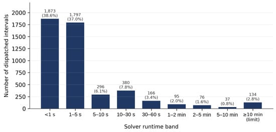
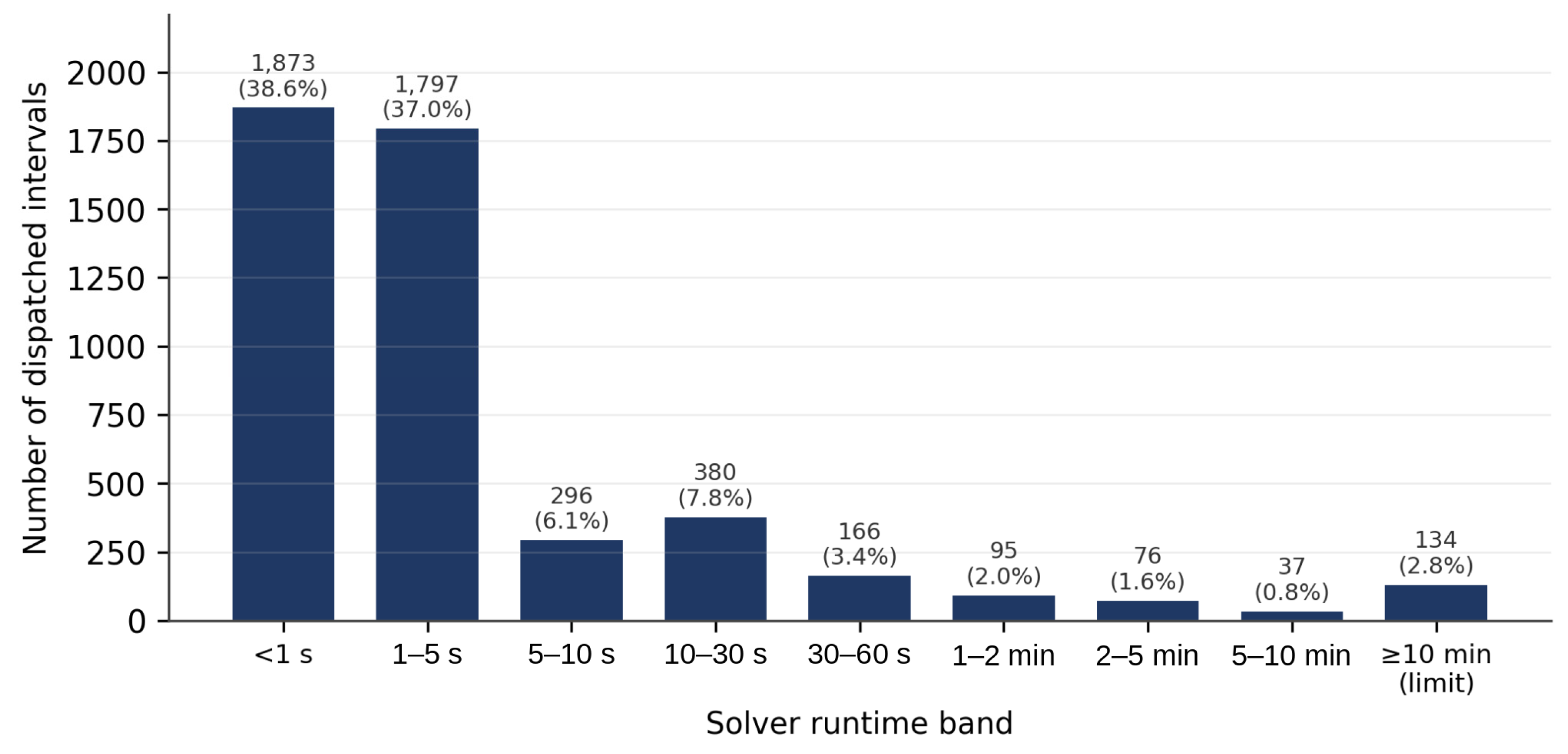
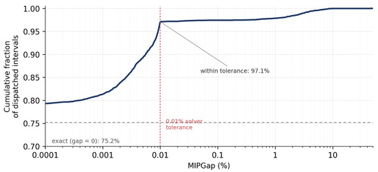
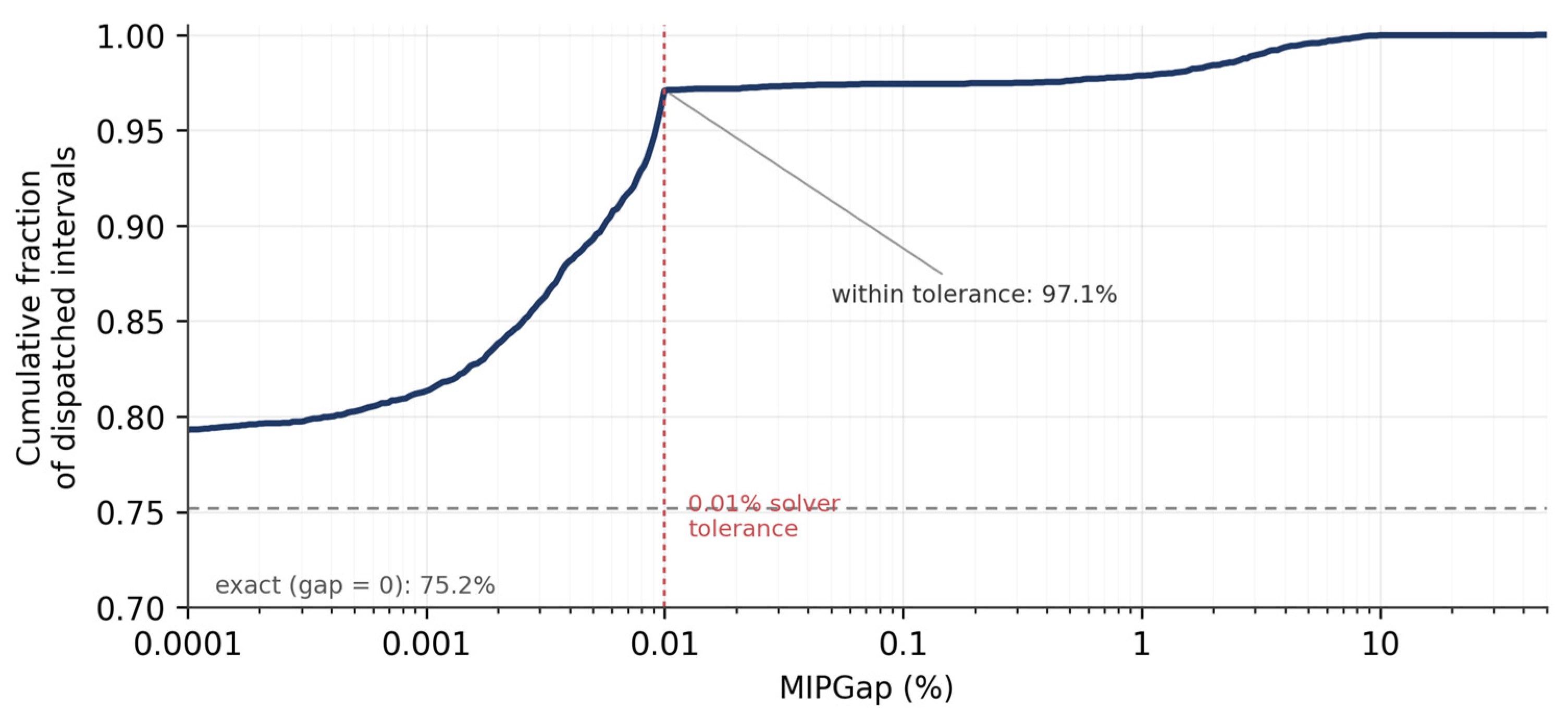
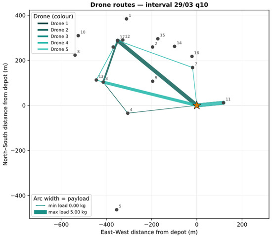
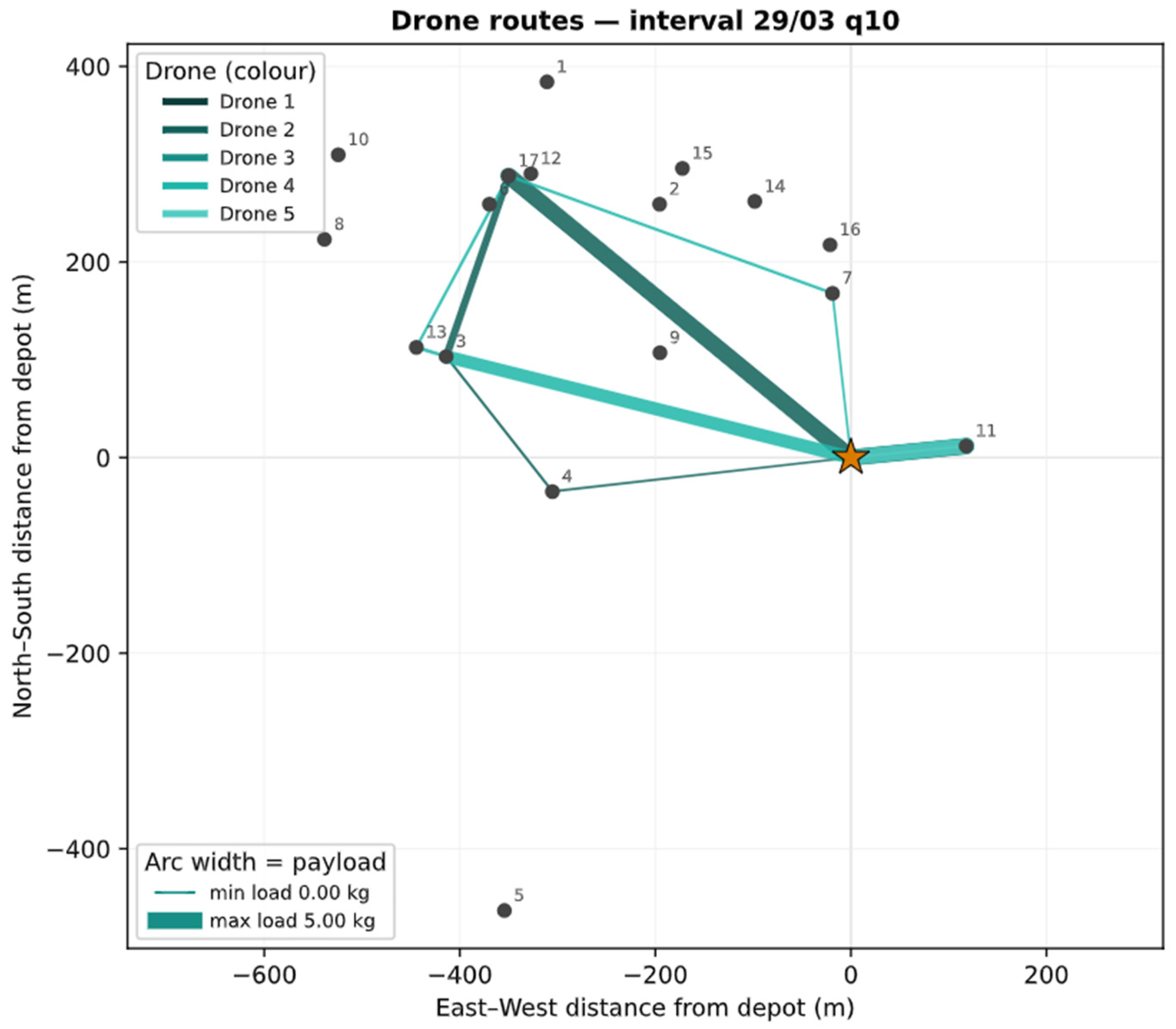
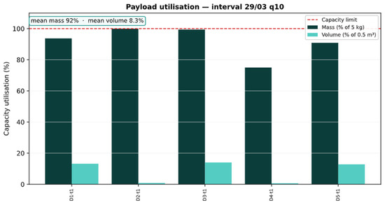
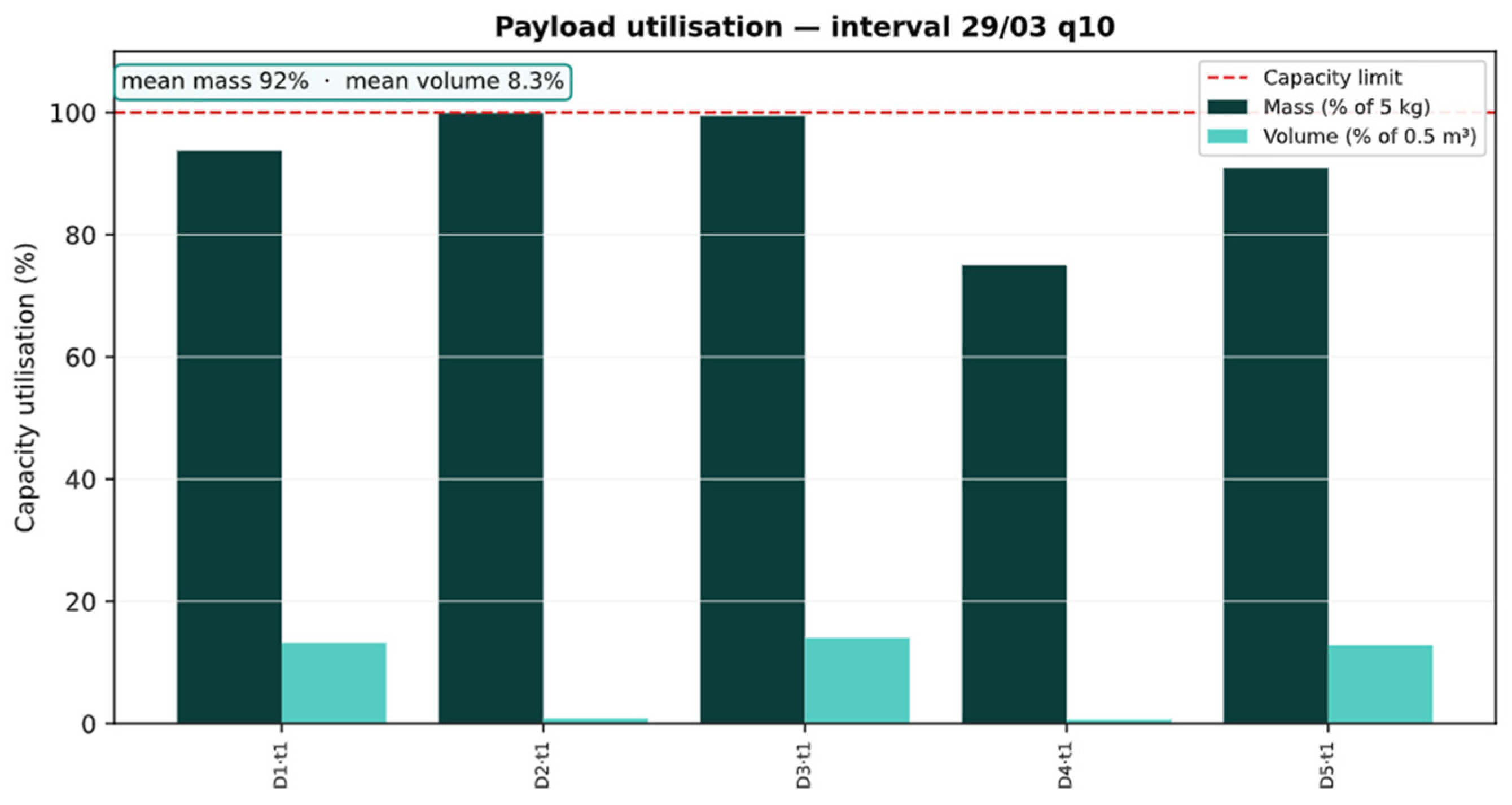
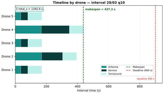
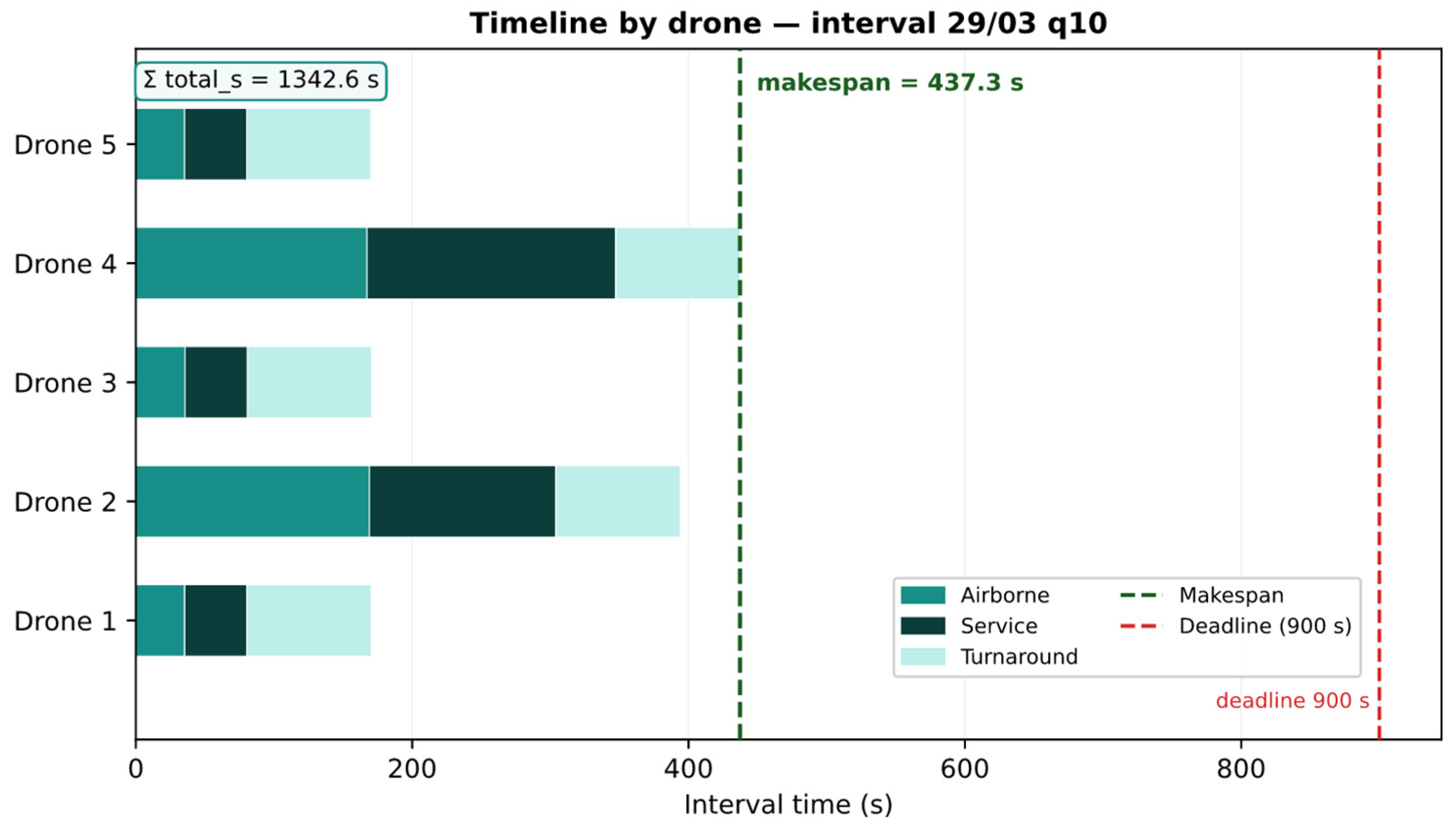
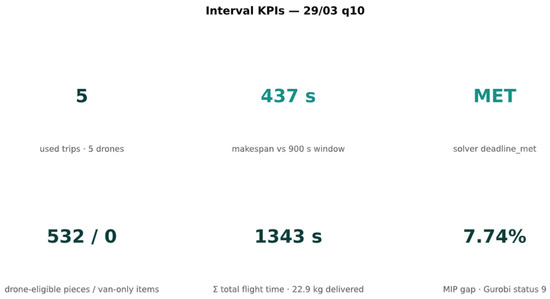
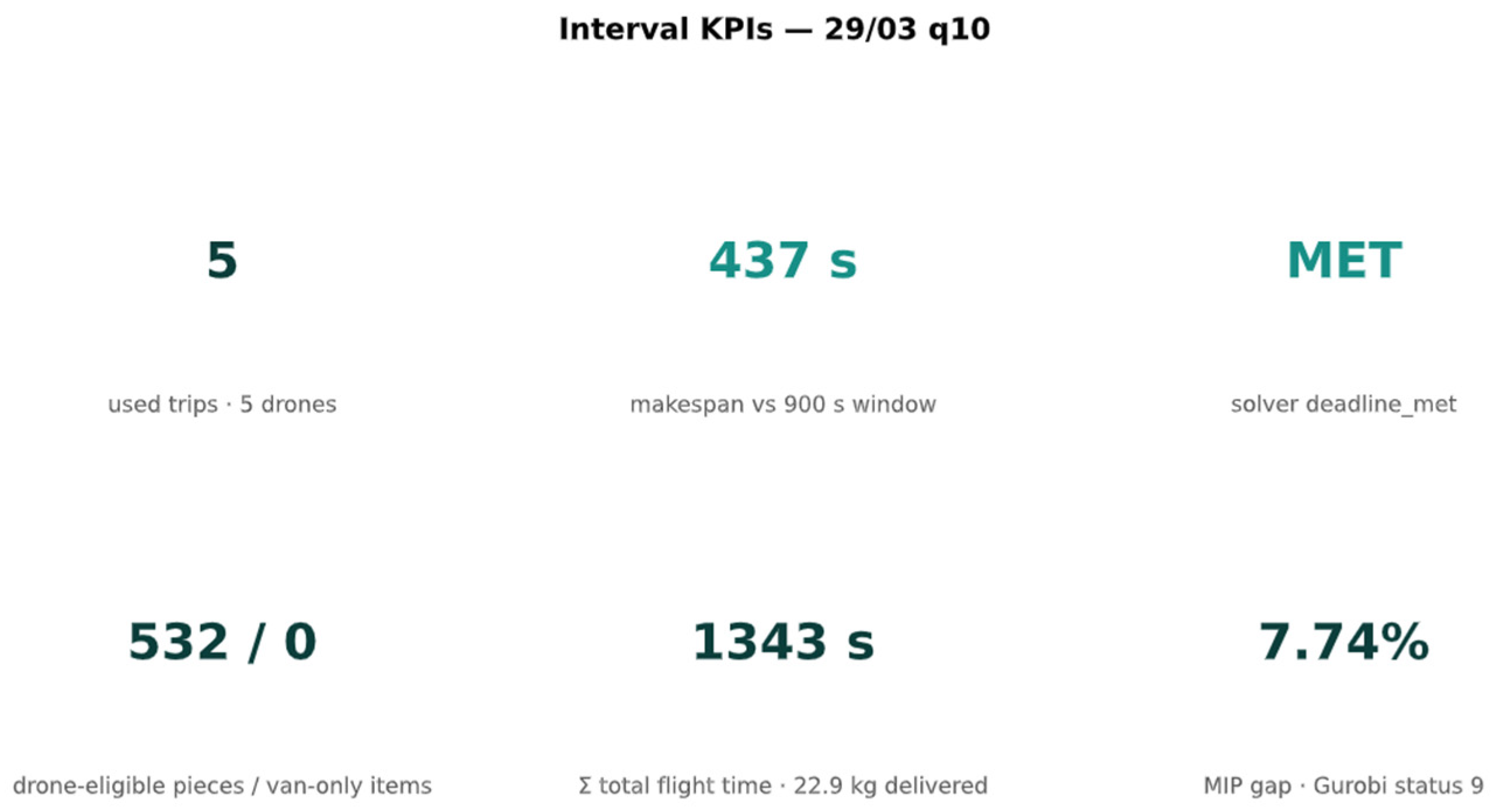
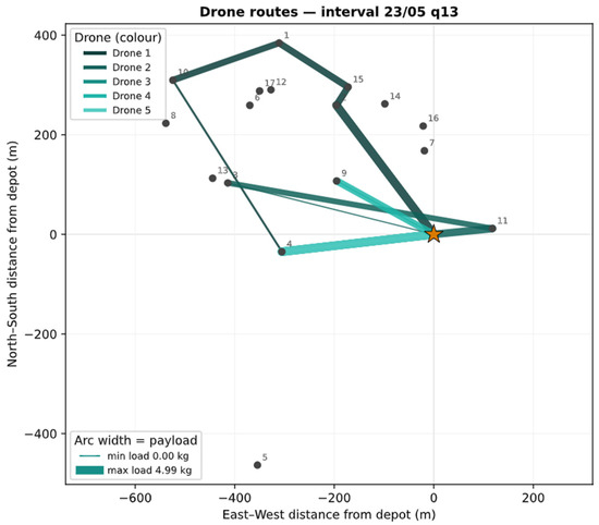
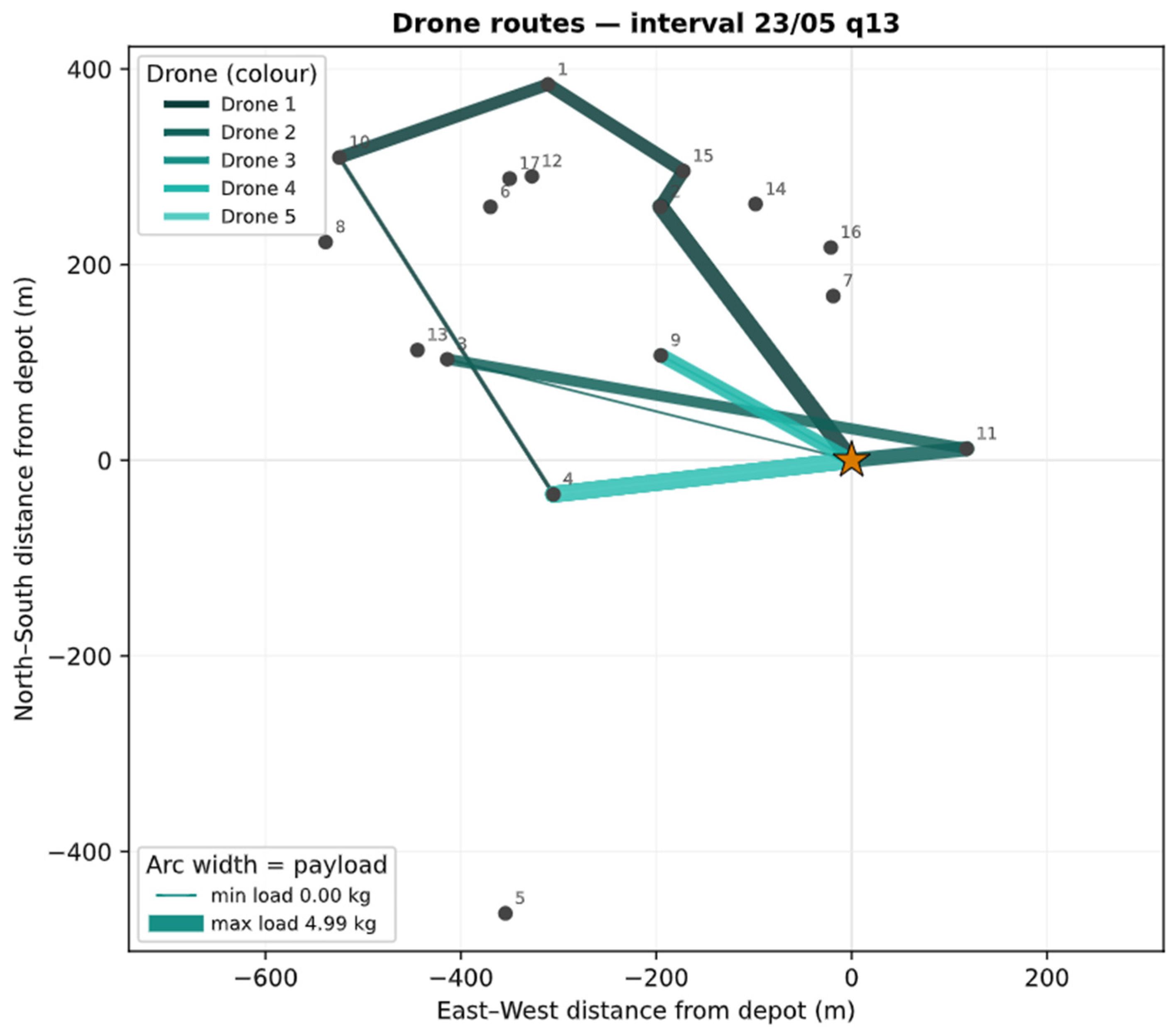
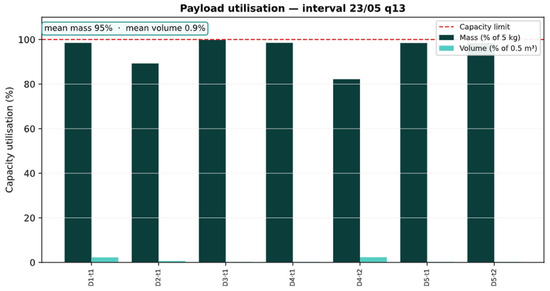
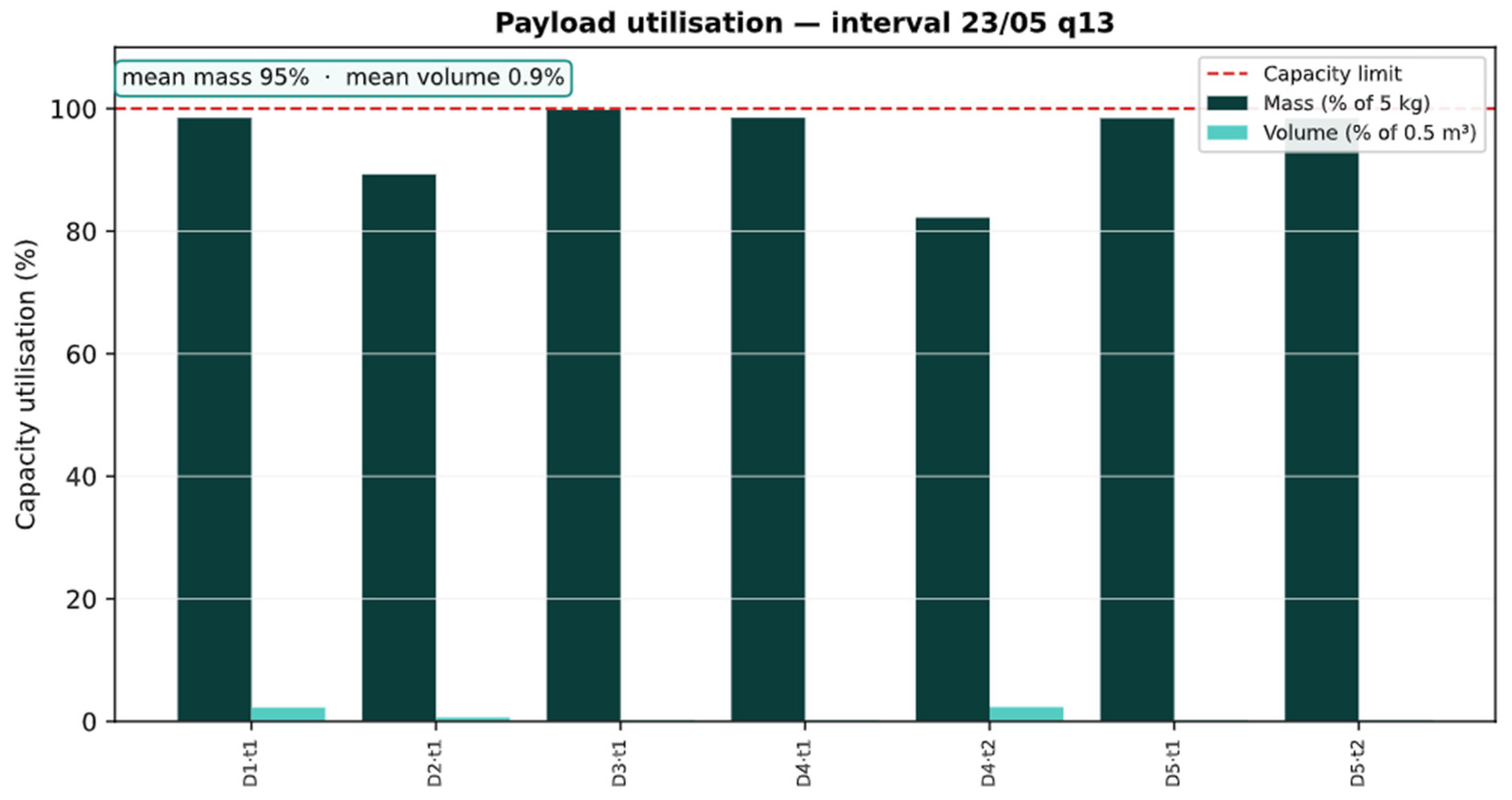
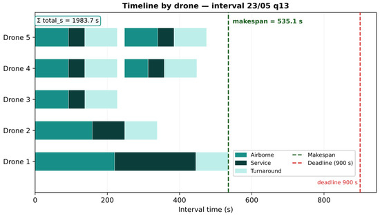
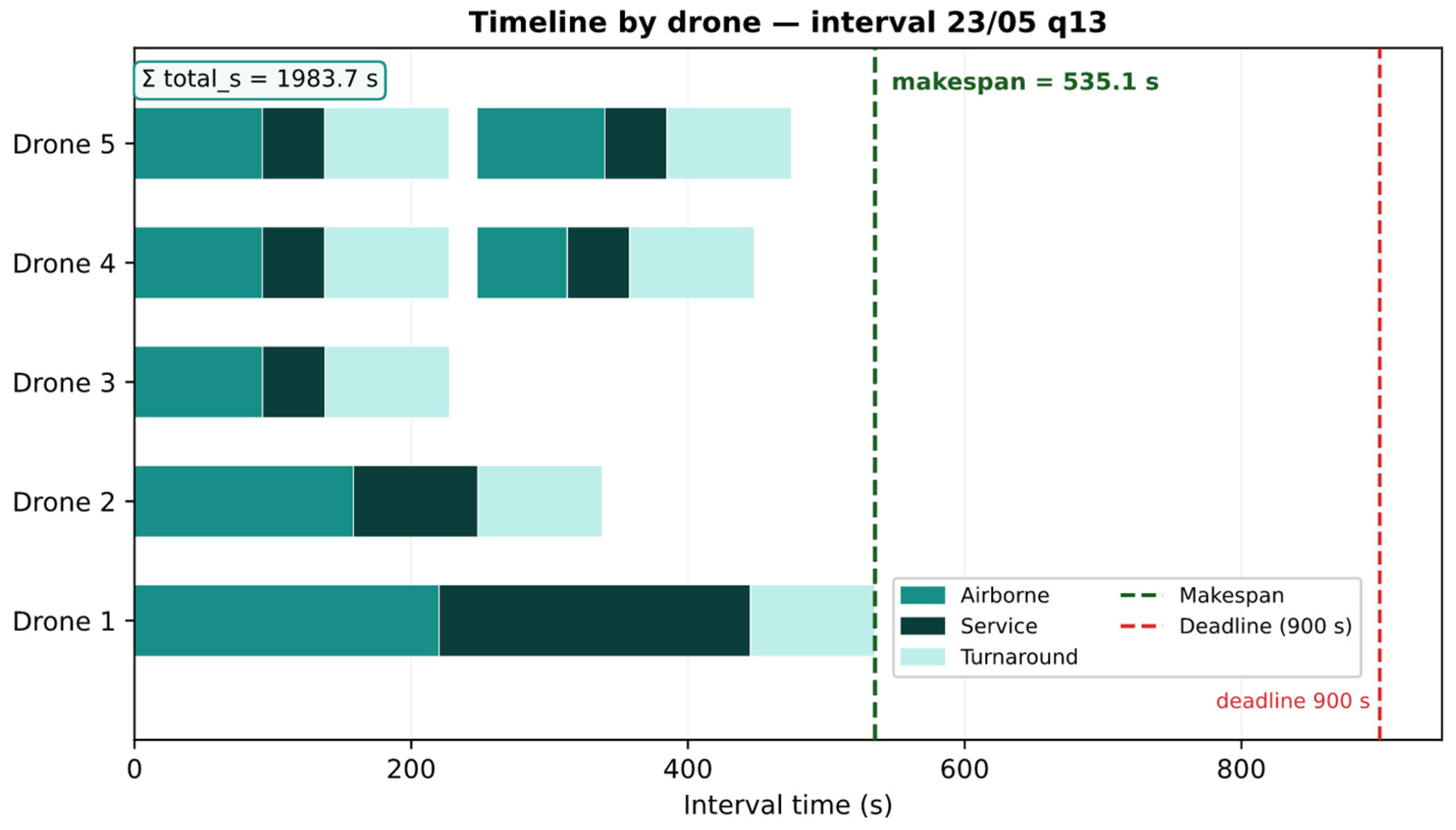
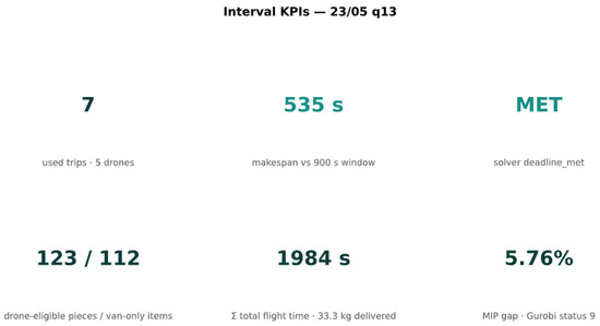
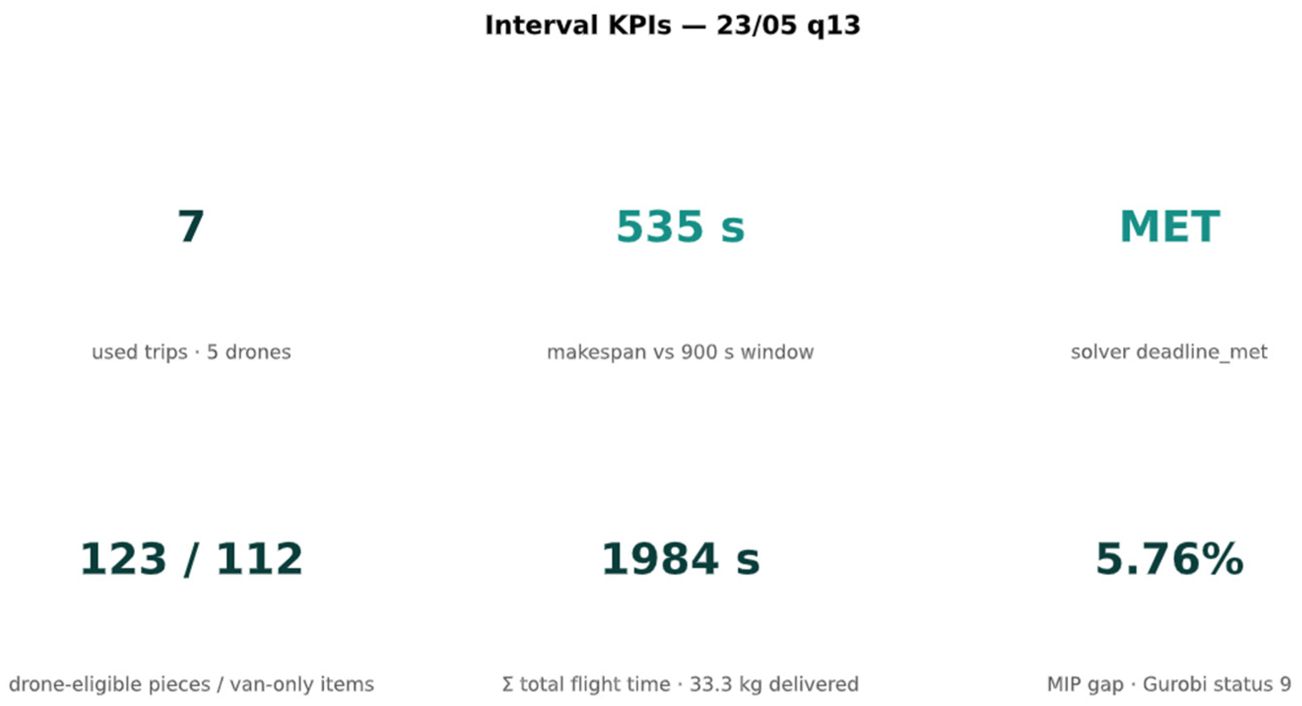
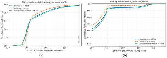
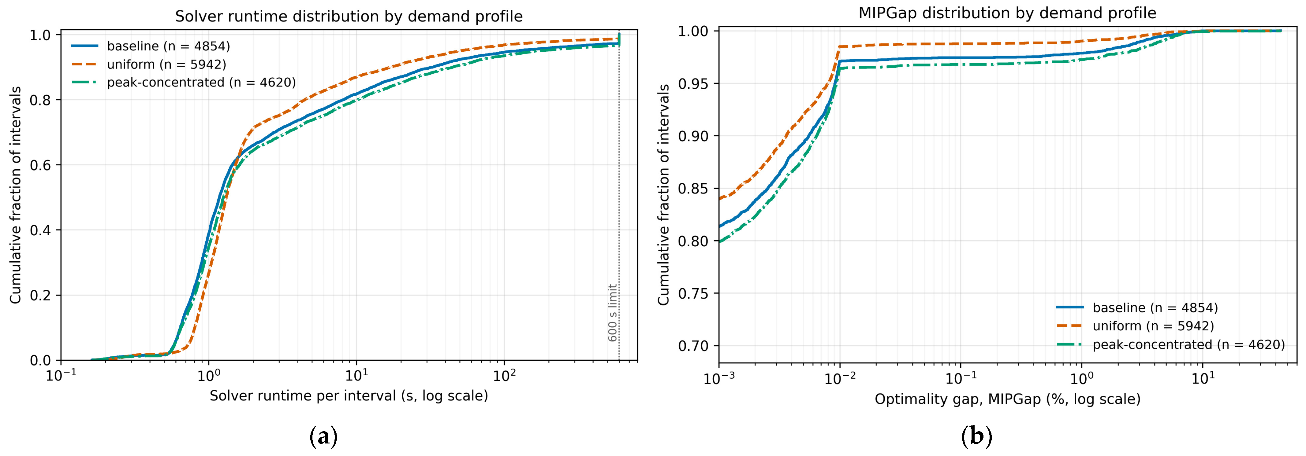

Disclaimer/Publisher’s Note: The statements, opinions and data contained in all publications are solely those of the individual author(s) and contributor(s) and not of MDPI and/or the editor(s). MDPI and/or the editor(s) disclaim responsibility for any injury to people or property resulting from any ideas, methods, instructions or products referred to in the content. |
© 2026 by the authors. Licensee MDPI, Basel, Switzerland. This article is an open access article distributed under the terms and conditions of the Creative Commons Attribution (CC BY) license.