


Abstract
Past Citi Bike rebalancing research has relied on optimization and geospatial models but has treated spatial and temporal structures separately, leaving a gap in understanding stations as long-term behavioral entities. This study exploits the frequent spatiotemporal structure in Citi Bike daily trip data and treats the station’s bike net flow rate (NFR) time-series as the study object. Stations are grouped into regimes using time-series clustering, cluster stability, and the spatial context surrounding each station. Stations were assigned operational roles based on their hourly NFRs and potential contribution to the rebalancing truck. A priority-queue-based heuristic routing (PQHR) algorithm is introduced to design a single-vehicle route that accounts for stations’ regimes, roles, rebalancing urgency, and priority during rush hours. Therefore, this study formally introduces the Station Behavior Regime Model (SBRM) that defines station regimes, rebalancing roles, and routing. The result achieved a >90% reduction in the number of stations with extreme bike accumulation or unavailability and reduced the NFR of affected stations by >30% in busy areas. The spatial context derived from station behavior modes suggests new ways to define neighborhood boundaries. The methodologies provide new avenues for rebalancing operations and routing plans across a broad range of station-centric transportation network studies.
1. Introduction
Bike-sharing programs have become a cost-effective, sustainable, and increasingly popular mode of transportation among urban dwellers in recent years. They usually come in two forms: docked bike-sharing and dockless bike-sharing. They are often referred to as micro-mobility systems because of their frequent use for short-distance travel as a complementary or alternative mode within public transportation systems. The bike-sharing business worldwide is projected to surpass $10 billion in 2026 and achieve a Compound Annual Growth Rate (CAGR) of 7.7% over the next 8 years [1]. Due to their significance for daily commutes and increasing integration into public transportation networks, as well as their congestion-reducing capabilities, lower emissions, and improved last-mile connectivity, stakeholders across sectors (municipalities, urban planners, and citizens) have shown strong support for deploying such transportation initiatives [1].
Citi Bike is the official docked bike-sharing program for New York City (NYC). Since its launch on Memorial Day, 2013, Citi Bike has emerged as one of the most popular micro-mobility systems in North America [2]. From 600-plus stations and 16 million trips in 2013 to over 2400 stations and 44 million trips in 2024, its success relies heavily on residents’ routine use, tourists’ passion for exploring the city, and the municipality’s public advocates and subsidies (Figure 1). Citi Bike encourages self-rebalancing to address bike and dock shortages through the Angel Biker program (in which customers ride bikes from crowded stations to those running low on bikes at discounted rates), thereby reducing rebalancing operational costs [3,4]. Despite its innovative and ambitious operational objectives, station expansion, and continued government support, performance has not progressed linearly, and the program did not turn a profit until 2023, precisely a decade after its launch (Figure 1) [5,6,7,8]. One of the reasons that kept certain riders away was the lack of bikes or docks available at busy stations during rush hours [8,9].
Figure 1.
Citi Bike Trip progression (2017–2024) and rebalancing performance (2014–2020). While annual bike trips have risen almost linearly in recent years, the number of bikes rebalanced each year has declined sharply after 2017. This unexplained sudden decline, the under-delivery of the rebalancing promise to the people and government of NYC, and the fact that a disproportionate amount of Citi Bike rebalancing research relies on data from before 2017 are the direct motivations for this project. (a) Citi Bike trips per year (2017–2024). (b) Rebalancing as a percentage of total trips [5].
Nevertheless, their approach of delivering reliable bikes to customers, minimizing operational costs, and emphasizing self-rebalancing efforts offers a compelling basis for framing this problem as research questions [10,11]. Since different numbers of bikes are at fixed locations at different times, what rebalancing operation can we perform to ensure each station always has bikes and docks available for customers [3]? This question is usually approached and theoretically solved using mixed-integer linear programming (MILP). Typical formulations jointly determine which stations to visit, pickup/drop-off quantities, vehicle assignment, and routing order. These formulations often lead to computationally NP-hard vehicle routing problems, limiting their usefulness for real-time decision-making.
In recent years, the Citi Bike rebalancing problem has also been addressed from various perspectives, including data analytics, optimization, operations, and urban planning. In 2017, Citi Bike adopted a study by O’Mahony and Shmoys (2015) and found temporary success with it [5,12]. However, the effectiveness of this algorithm appears to have declined since 2019, potentially reflecting broader changes in system dynamics associated with station network expansion, internal business-priority and leadership changes, and increasing operational complexity [5,9]. These observations suggest that the behavioral structure of the Citi Bike program may no longer be adequately captured by assumptions derived from earlier operating periods. Therefore, this study revisits the rebalancing problem using historical trip data (2017–2024) and a more diverse set of tools, in addition to MIO, to develop a new routing algorithm. Rather than focusing solely on short-term inventory optimization, we hypothesize that Citi Bike stations exhibit a persistent behavioral regime that can be identified from historical bike net-flow patterns and exploited to guide practical rebalancing operations. The objective is to develop a lightweight, interpretable framework that can generate reliable, small-scale rebalancing routes for truck-based operations. The primary contribution of this study is the introduction of a station-level behavior-driven classification framework that integrates temporal, spatial, and operational information into a computationally lightweight heuristic-based rebalancing strategy.
Thus, this paper proposes the Station Behavioral Regime Model (SBRM). SBRM characterizes stations by their regimes, defined by three long-term properties. They are the station-level daily bike net-flow behavior patterns, behavioral stability, and spatial context. These regime definitions are combined with hourly operational roles derived from net-flow rates to guide a priority-queue-based routing algorithm. SBRM is a data-driven, machine-learning-based heuristic framework that exploits the persistent spatial-temporal behavior patterns of stations. By defining and assigning the station’s regimes in advance, the proposed Priority-Queue-based Heuristic Rebalancing (PQHR) algorithm constructs a practical rebalancing route with minimal online computation, rather than relying extensively on mathematical optimization.
The whole SBRM framework is intuitive and easy to compute. All regime and operational role assignments can be derived from data from about a year ago to ensure they align with the desired station behavior pattern and seasonality. Doing so shifts much of the computational effort from operational time to an offline preprocessing stage. Such an approach also provides insights into potential expansion plans in underprivileged areas of NYC, where large-scale transportation systems (such as the subway, which can take decades to build a single line) are lacking. SBRM is also useful for site selection in cities without a docked bike-sharing program yet, helping them identify the most sensible locations and the optimal number of docks to start with. It also sheds light on dockless bike-sharing cities around the world, showing that such programs can be productive and convenient without sacrificing the neat, clean look of pedestrian walkways.
2. Literature Review
In this section, we review common approaches to directly addressing Citi Bike rebalancing problems, as well as the relevant studies that inspired our approach.
2.1. Closed-Form Model-Building
The Citi Bike program has open-sourced and professionally maintained its daily bike trip data since July 2013, two months after the program’s inception. Doing so has generated waves of theoretical and practical research ideas and equipped closed-form model building for more than a decade. This section reviews several outstanding closed-form models designed specifically for the Citi Bike rebalancing problem.
Schuijbroek et al. derive Citi Bike station service levels and net bike and dock demand from inventory frameworks, and use a mixed-integer linear programming (MILP) approach to minimize the makespan (travel time between stations) among feasible stations, thereby restoring system equilibrium [13]. O’Mahony and Shmoys’ model, which Citi Bike has adapted since 2017, optimizes station inventory levels during rush hours while accounting for operational constraints such as travel time and service coverage [12]. Liu et al. (2016) further integrate station-level demand prediction with route optimization, distinguishing weekday and weekend demand patterns to improve operational planning [14].
In addition to the integer-programming-based optimization, many other closed-form models have incorporated operational heuristics, incentive schemes, and stochastic processes into rebalancing design. Freund et al. (2020) minimize dissatisfaction by using decomposed integer-programming subproblems and localized routing strategies [15]. Chiariotti et al. (2018; 2019) model station dynamics using a Birth-Death Process and propose incentive-based user redistribution to reduce congestion pressure [16,17]. Tedeschi (2016) emphasizes that station load factors and temporal availability patterns can directly guide rebalancing efforts [3]. Sun et al. (2023) used a density- and grid-based clustering algorithm with multilevel density thresholds to locate rebalancing nodes based on self-balancing degree, and used a neural network-based approach to predict rebalancing pressure and to develop a rebalancing route [18]. More broadly, O’Brien et al. (2014) highlight bike-sharing systems as valuable sources of mobility and urban planning data beyond transportation operations alone [19]. Collectively, these studies demonstrate that station-level behavioral patterns are central to effective rebalancing design.
Although these studies demonstrate that station-level demand patterns play a central role in rebalancing, most use them primarily to parameterize optimization models rather than to model long-term station-level behavioral characteristics. Instead of employing optimization strategies, this study treats recurring station behavior as the primary analytical focus and leverages it directly to construct heuristics for route construction, using data engineering and clustering techniques.
2.2. Geospatial and Temporal Analysis of Citi Bike Stations Trip Data
A related but distinct line of inquiry in rebalancing studies concerns geospatial analysis of Citi Bike trip data. Although they do not directly develop models for rebalancing, they are either conducted with rebalancing in mind or provide insights and guidance on addressing it [3]. Previous studies have used GIS visualization, community detection, and 3-D flow mapping to identify recurring spatial patterns within the Citi Bike network [5,20,21,22]. These studies consistently show that stations with similar temporal demand profiles tend to cluster geographically, such as residential areas with strong early-morning pickup demand and business districts with strong late-afternoon departures [3,21].
Another line of research analyzes Origin-Destination (OD) flows during peak periods to identify travel corridors and inform rebranding strategies [21,23,24,25]. While OD analyses could be effective for understanding network-wide flows, they would require continuous monitoring of evolving OD patterns to identify a plausible rebalancing route in real time, making them infeasible for real operations. Thus, this paper addresses this gap by shifting attention from OD analysis to station-focused analysis and seeks to leverage more consistent patterns in stations’ behavior to develop a single knowledge- and data-based model, rather than sequentially updated layers, to guide real-time operations.
In parallel with these efforts to identify geospatial patterns, a substantial body of research has examined temporal patterns and longitudinal analyses in the Citi Bike literature. Past research can be grouped into two branches. The first is stations’ macro-overview of trip volume patterns throughout the year, with ridership peaking in the summer and troughing in the winter [21,26,27]. The second is the stations’ daily ridership, showing distinct patterns across hours of the day; in particular, weekends and weekdays exhibit different daily patterns [28,29,30].
At the macro level, temporal and longitudinal studies of the Citi Bike network have found that Citi Bike station-level demand exhibits strong seasonality, is highly sensitive to daily weather conditions, and that weekend and weekday demand profiles differ drastically [21,23]. Meanwhile, external shocks, such as COVID-19, could cause significant disruptions to existing regular patterns [31,32,33]. However, almost all the literature agrees that Citi Bike station-level demand follows a long-term pattern that remains highly stable and predictable, motivating our focus on identifying and substantiating recurring behavior regimes rather than short-term fluctuations [26,27,28,29,30].
At the micro level, station behavior exhibits distinctive features, but many of these features show similar daily trip peaks and troughs; therefore, daily Time Series (TS) clustering is a worthwhile approach to investigate station behavior [17,30]. In particular, weekday time series typically show patterns more closely aligned with residents’ 9–5 daily schedules, whereas these patterns wane on weekends [21,30]. Inspired by the recurring and elucidating temporal patterns, we are motivated to treat each station’s daily time-series as the unit of analysis for clustering-based behavioral modeling. We will discuss the most commonly used TS clustering algorithms and their theoretical contributions in the next section.
Beyond these data analyses, various research efforts have also mentioned the spatiotemporal context of the Citi Bike sharing system, reinforcing the idea that rebalancing operations should be broken down into manageable areas. More broadly, recent studies have incorporated built-environment and place-based information to redefine neighborhood boundaries based on urban functionality rather than administrative divisions [34,35,36,37,38]. For example, Marti et al. (2021) propose using Google Places Data and a series of rigorous processing steps for land-based classifications, and clustering areas by place functionality to redefine the neighborhood boundary [34]. Such an approach proves more effective at capturing demographics and human behavior than an administrative neighborhood boundary. Inspired by the idea, this paper aims to leverage the abundant spatiotemporal patterns in the Citi Bike system to develop a new neighborhood boundary [34,39]. By doing so, we intend to design better neighborhood boundaries that incorporate mobility patterns, ultimately improving the rebalancing routing algorithm and expediting rebalancing operations.
2.3. Recent Advancements in TS Clustering Techniques
The TS clustering algorithm clusters the time-series objects based on their magnitudes and shapes [40,41]. This gives the approach a strong connection to traditional clustering methods, including K-means and kernel-based algorithms such as K-shape [41,42]. In traditional clustering algorithms, the input is a number or set of numbers, usually representing geospatial distance or time differences. In TS clustering, the distance is calculated from the difference in trip volume at each corresponding time step.
K-Means-TS-clustering (Euclidean) is a centroid-based method that uses the exact pairwise differences between points to measure similarity. K-means Dynamic Time Warping clustering measures similarity by finding the optimal alignment between two temporal sequences that may vary in speed or timing, using the Dynamic Time Warping (DTW) technique [42,43]. The DTW is particularly effective because it minimizes the distance between signals when the similarity occurs at slightly different time points [43]. In 2017, Soft-DTW, a differentiable loss function for time-series, emerged as a gradient-based learning-friendly algorithm compared to traditional DTW and has since been shown to be even more accurate for clustering time-series [44].
Subsequent centroid-based TS clustering studies shift their focus from deriving similarity by finding optimal matching time steps to forming clusters with an emphasis on the shape of the time-series objects. One of the most prominent such algorithms is K-shape clustering [45]. Unlike K-means, K-shape clustering groups series based on shape similarity rather than point-wise distance, using a shape-based distance (SBD) and a centroid-based distance that relies on the normalized cross-correlation technique to identify similar patterns. Therefore, it excels at ignoring certain amplitude variations and potential noise. It is known to be more efficient and scalable in practice. The K-shape also appears to be more effective for abnormality detection [46].
Another school of thought in TS clustering is kernel-based clustering, specifically the Global Alignment Kernel (GAK) [44]. GAK measures similarity by aggregating all possible alignments between two sequences. In unlined standard K-means, explicit centroids are not computed; instead, the algorithm relies on the computed kernel matrix to account for time shifts. In practice and performance, it serves as a bridge between Soft-DTW and traditional kernel methods, thanks to its differentiable, parameter-adjustable techniques. By computing kernels over all possible alignments between two sequences, it maps the data into a higher-dimensional feature space where non-linear patterns may become linearly separable, thereby potentially forming more accurate clusters [47,48].
All these TS clustering techniques prove effective and have specialized applications across different domains. Since this is one of the first times a thorough application of TS clustering has been used on Citi Bike historical trip data, this paper will experiment with, explore, and compare the effectiveness of the five aforementioned TS clustering techniques on Citi Bike trip data, as well as the convenience they provide for rebalancing operations. Hopefully, such thorough experimentation and documentation will inspire future research efforts on TS clustering and mobility data.
2.4. Rebalancing Route Designs and Realizations
In addition to the MILP optimization mentioned in the model building above, route optimization spans a wide range of academic disciplines, including operational engineering, business management, mechanical engineering, and computer science (graph theory and network analysis). As mentioned in Section 2.1, designing a rebalancing route that accounts for multiple vehicles and routes was challenging, especially given the systems’ ever-changing dynamics. Therefore, this section focuses on algorithms and logistics for single-vehicle, single-route techniques.
Classical routing algorithms, such as Dijkstra’s shortest-path algorithm and Traveling Salesman Problem (TSP) formulations, provide useful theoretical foundations for rebalancing design [49,50]. However, their direct application is challenging because they focus on finding the shortest path between stations, which deviates from the core requirement of the rebalancing problem. Furthermore, in the Citi Bike system, station states change dynamically over short time intervals, making globally optimal routes unstable and computationally expensive to recompute in real time.
Many recent studies on rebalancing routing algorithms have drawn inspiration from both Dijkstra’s and TSP research, incorporating queue-based and greedy graph-building elements. A priority-queue-based rebalancing algorithm typically constructs a queue based on imbalance severity and station distance, and the rebalancing vehicle is designed to solve this dynamic queue-clearing problem under cost constraints to cover as many stations as possible [51,52,53]. This approach simplifies the routing problem by greedily assigning the most urgent station, minimizing travel costs, and ensuring bike availability on the rebalancing fleet [50]. Along the same lines of reasoning, discussions have centered on simplified TSP-inspired algorithms—several works have proposed greedy constructive heuristics that use a distance-efficient backbone (TSP-based) and add stations based on rebalancing pressure to carve out the longest capacity-feasible subpaths until all stations are served [54,55]. Finally, more generic, logistics-based heuristics for rebalancing routing algorithms have also been proposed to determine which stations to add to their dynamic routes and how many bikes to either drop off or pick up [56]. In our study, we believe it is key to adapt a simplified version of a priority queue and heuristic rebalancing routing strategy, while incorporating the key spatiotemporal structure derived from daily trip TS clustering, to mitigate rebalancing pressure within the systems.
2.5. Consolidated Overview and This Study’s Contributions
After reviewing the state of the art of models and analyses of Citi Bike trip data to address rebalancing problems, we believe there is a need for a model that leverages the evident spatiotemporal structure of the Citi Bike sharing system, as such a structure has been found in bike sharing programs in other cities [57]. A recurring limitation across the state of the art is that many studies used clustering methods, but none simultaneously captured the coexisting spatiotemporal structures within the system. They either categorized stations by temporal snapshots of varying rental and return rates or by geospatial distances and connectedness. Additionally, almost all previous Citi Bike station studies have monitored and analyzed routine demand shifts at certain stations and the lack thereof at others throughout the day; however, they have not adequately capitalized on this pattern. Hence, a common struggle with these existing models is that rebalancing routes often focuses on the hotspot stations as a compromise, leaving out or failing to fully leverage stations with different behavior patterns. Yet, the gap is not insurmountable, given recent advancements in TS clustering. We believe that a rebalancing model using machine learning and a dynamic Priority-Queue-based TSP heuristic would be feasible and could greatly alleviate pressure on Citi Bike’s rebalancing operations.
Specifically, our contributions to this field are fivefold. First, we compute each station’s hourly net flow rate to capture bike/dock demand and the pressure for rebalancing. Second, rather than relying on spatial clustering alone or on hourly demand clustering, we classify station types by treating each station’s daily net flow-rate time series as the primary unit of analysis. Third, we combine place-based and station-level data to develop a more refined functional definition of NYC neighborhood boundaries that better supports rebalancing goals and route design. Fourth, we identify hourly operational roles for stations based on their cluster membership, stability, and spatial context. Finally, we apply dynamic-priority-queue-based TPS heuristic routing algorithms to produce a single-vehicle, single-route rebalancing solution and validate it against real-world data.
3. Methodology
3.1. Data
3.1.1. Citi Bike Historical Data
Historical Citi Bike trip data were collected from the Citi Bike website, which is maintained and open-sourced by Citi and Lyft [58]. The format and attributes of the trip data changed once, towards the end of 2019, within our study period, from 2017 to 2024. Before 1 January 2020, the dataset included each rider’s birth year, gender, and bike ID; however, the trip data lacked primary keys. After 1 January 2020, each trip had a primary key indicating whether the rented bike was a classic or an e-bike, but it did not include the rider’s birth year, gender, or bike ID. Therefore, the first step we took was to create and assign primary keys to the trip data from1 January 2017 to 31 December 2019. We also created a new attribute to store the trip’s starting and ending station, “start_end_pair”, for easier Origin-Destination (OD) pair retrieval and analysis (Table 1).
Table 1.
Citi Bike historical trip data.
3.1.2. Station-Wise JSON Data
Deriving station capacity required combining two publicly available JSON data feeds, since neither source covered all stations in the historical trip dataset. Both feeds were retrieved on 2 January 2026, converted to CSV, and analyzed in a Google Colab notebook (version 7.6.0). All station status values reflect that single snapshot. We first extracted capacity directly from the station information JSON’s existing capacity column (Table 2), which covered approximately 87.13% of stations in the trip dataset [58,59]. Therefore, we also used Station Status JSON to approximate station capacity for active stations by summing the numbers of available and disabled docks and available and disabled bikes for each active station (Table 2) [59].
Table 2.
Citi Bike real-time station status and station information data.
Since none of these datasets (Citi Bike historical trip data and the two JSON data feeds) use the same name for “station ID” across datasets. We merge each pair of datasets with their shared station ID, under different names, one step at a time. Table 3 shows all station identification data available for each dataset, and entries in the same color share the same format and contain overlapping station IDs. Therefore, we first merged the Citi Bike historical data and the Station status JSON based on their shared station IDs, “station_id” and “legacy_id”, respectively. Then, we merged the Station status JSON and Station information JSON based on their shared station ID, called “station_id” and “external_id”. Finally, we merged the two datasets using the identified station IDs and retrieved all station capacity data from both datasets. Eventually, 96.57% of the stations in the trip data’s capacity was derived and recovered. Trips with stations that lacked available capacity information were excluded from the analysis that follows. After integration and cleaning, the final station dataset contained 2162 unique stations with valid capacity estimates available for analysis.
Table 3.
Three Citi Bike datasets’ geographical identifiers.
3.2. Method
This section introduces the data engineering procedures, station behavior regime definitions, operational roles, and the Priority-Queue-Based Heuristic Rebalancing (PQHR) algorithm. Together, these elements constitute the Station Behavior Regime Model (SBRM). We first introduce a general framework based on historical Citi Bike data from 2017 to 2024 (Section 3.2.1, Section 3.2.2, Section 3.2.3, Section 3.2.4, Section 3.2.5 and Section 3.2.6). We then apply the framework to a specific case study in which rebalancing routes are designed using 2023 data and evaluated on 2024 data using PQHR, and we compare its performance against baseline algorithms and ablation variants (Section 3.2.7). To preserve the out-of-sample nature of the evaluation, 2024 data are excluded from the estimation of reference clusters, dominant behavior modes, stability classification, and spatial context. Finally, Section 3.2.8 summarizes the complete SBRM framework.
3.2.1. Data Engineering and NetFlow Rate (NFR) Time-Series Preparation
We selected Citi Bike historical data from 22 March to 21 April every year from 2017 to 2024. The annual trip data show strong seasonality, with summer being the busiest. Summer and winter months tend to be less regular or stable due to the academic calendar and shortened in-office working hours. A month in mid- to late spring appears to be most representative of “typical” daily usage, as bike trips tend to increase with warmer weather, and students and professionals have regular in-person working hours. Since the NYC Pause order was issued on 22 March 2020, data from 22 March to 21 April (31 days) were selected to enable a better Year-Over-Year comparison, particularly to observe any abnormalities in 2020 [60]. Notably, when generating the final averaged station behavior panel data, 2020 data were excluded to reduce the impact of such rare external shocks. In the rest of this study, each year’s 22 March–21 April data are referred to by that year’s name for conciseness.
Data engineering is particularly crucial for transforming the raw Citi Bike trip data into station-hourly-net-flow panels suitable for time-series clustering, since the raw dataset represents each trip as a row in a bike-, start-station-, and end-station format. Raw trip records were first aggregated into station-hour inflow and outflow counts for each year. Stations’ capacities were merged from the cleaned station JSON files mentioned in Section 3.1.2. A total of 744 (31 days × 24 h) rows were generated for each station present in each year panel. The weekday and weekend subsets were then extracted using the actual number of dates (Table 4). For each station—both weekday and weekend versions—the daily 24 h panel (a time series of inflows and outflows) was computed as the average of hourly inflows and outflows over the respective days. Therefore, the magnitude of these metrics appears smaller than the actual values, with fewer extreme values than in the actual data when sent to clustering and downstream analysis. This effect would influence how parameters and thresholds were selected during the build-up of the routing algorithm. For hours when no trips were observed, the station-hour inflow and outflow were set to zero.
Table 4.
Summary of Citi Bike station-hour dataset construction across the study period.
Subsequently, all yearly panels were merged by station name to form two complete station-hour panels, one weekend and one weekday, for all years, excluding 2020. Thus, the station-hourly inflows and outflows were aggregated by averaging over the 7 years. The 2020 data were omitted from the reference clustering because regular daily human behavior changed during March–April 2020 due to strict “stay at home” orders and the directive that non-essential workers work from home; including them would have added more noise to the clustering [60]. This consolidated dataset was used for 2 purposes: (1) to generate the reference cluster assignments so that each individual year’s cluster assignment can be aligned across different years; (2) to find the dominant behavior mode for each station, through the longitudinal analysis of the year-to-year cluster changes in each station, if any.
Since we treated each station’s hourly net flow rate time-series as the study objects, which were used to identify station bike rental behavior patterns, we further defined net flow rate as follows:
where are the inflows per station per hour , and are the outflows per station per hour . is the net flow at station and hour , Capacitys is the station’s maximum capacity, and is the net flow rate at station and hour . For annual analyses, clustering was performed individually on each year’s station-level 24 h profiles, for weekdays and weekends. Positive NFRs indicate a net accumulation of bikes at a station, while negative values indicate a net depletion.
Critically, this process trimmed the raw trip data (21 March to 20 April for 8 years) from 18.8 million rows into station-hour panels totaling 7.5 M records. These records were subsequently aggregated into station-level 24 h weekday and weekend profiles, yielding approximately ~627–2162 time-series per year and 2162 time-series in the final 7-year reference dataset. These procedures transform historical bike trip data into station-level bike demand data. Doing so enabled the creation of appropriate datasets (yearly and consolidated) ready for time-series clustering.
3.2.2. Station Trip Behavior Clustering
This study selected and evaluated five of the most frequently used time-series clustering techniques: TimeseriesKMeans Euclidean, TimeseriesKMeans Dynamic Time Warping (DTW), TimeseriesKMeans SoftDTW, KernelKMeans Global Alignment Kernel (Gak), and KShape. We then selected the one with the highest silhouette score for further analysis. Due to the large volume of data over 8 years, we used only the 2024 weekend and weekday station-trip data for experiments. Intermediate results (e.g., clustering results) are presented in this section rather than in Section 4, as the details of the SoftDTW implementation are included here, and Section 4 will focus more on the station regime and PQHR rebalancing results.
TimeseriesKMeans SoftDTW was the best-performing clustering algorithm on weekday data, and TimeseriesKMeans Euclidean was the best on weekend data. Since SoftDTW performed better overall on both weekends and weekdays, we used it as the clustering algorithm for both datasets. The full comparison is in Table 5. A brief mathematical explanation of why SoftDTW appeared to be the most appropriate algorithm is provided in Appendix A.
Table 5.
5 time-series clustering algorithm silhouette scores.
The number of clusters for the weekday and weekend datasets was determined using the Elbow method and human interpretation. We determined the number of clusters for weekdays and weekends using DTW rather than SoftDTW, because DTW has a much shorter computation time and shares similar underlying logic (Figure 2). We chose 3 and 2 clusters for weekdays and weekends, respectively.
Figure 2.
Elbow method with K-means DTW on Weekday and Weekend data. Although weekday data could use either 2 or 3 clusters based on the Elbow method result, we decided on 3 clusters for better human interpretations. For weekend data, 2 clusters were appropriate. (a) Elbow method for weekday data. (b) Elbow method for weekend data.
Before clustering, all station time-series were standardized to zero mean and unit variance using the TimeseriesMeanVariance function from the tslearn Python package (tslearn 0.7.0; Python 3.12.12) [61]. SoftDTW clustering was implemented on the individual yearly datasets and also applied to the consolidated station-hour panels to create a reference clustering for the individual yearly station cluster assignments. For weekday data, it was applied using TimeseriesKMeans with k = 3, a maximum of 50 iterations, default smoothing gamma (=1.0), and a fixed random seed of 42 [61]. Pairwise SoftDTW distances were computed internally by the tslearn implementation during clustering optimization [61,62]. No separate distance metrics were precomputed, and default SoftDTW parameters were used. For the weekend data, everything was the same except k was set to 2.
Each station from each year was assigned a cluster. Because cluster labels are arbitrary and the same number may represent different temporal patterns across years, the Hungarian assignment algorithm was used to align yearly clusters with the reference clustering by minimizing the total distance between cluster centroids [63]. This ensured that clusters with similar temporal shapes received consistent labels across years. Additionally, for each year’s clusters, we computed confidence scores based on the Softmax probabilities of their match with the reference clusters.
A complete data engineering workflow is summarized in Figure 3. Finally, we used matplotlib, a Python plotting package, to visualize clusters and clustering patterns over the years.
Figure 3.
Data processing pipeline from raw Citi Bike trips to time-series clustering input.
3.2.3. Station Behavioral Regime Definition
We define a station’s regime to capture its long-term characteristics and help design rebalancing routes, based on three factors: (1) TS clustering results, or behavior mode; (2) the stability of its assigned cluster, or behavior stability; (3) the spatial context of the station. We use the term “behavior mode” to refer to the interpreted TS cluster assignment going forward.
Firstly, each behavior mode was assigned a human-readable label, such as “morning accumulating, late afternoon depleting station”, “morning depleting, late afternoon accumulating station”, and “all-day diffusing station”, etc. Each label signifies the intra-day demand profile captured by its corresponding TS cluster.
Secondly, a station’s behavioral stability was determined by the frequency with which it was labeled as its dominant cluster over time across the available study years. A dominant cluster is the cluster label most frequently associated with a station over time. The criteria are expressed as:
where is the count of year-to-year transition, is the cluster label of stations in year t, and is the indicator function. Cluster changes were calculated as year-to-year transitions. We define a station’s behavior mode stability based on these criteria:
Changes occurring during 2020 were excluded from the stability assessment. Moreover, if a station transitioned to a new cluster in 2020 and remained in that cluster thereafter, the transition was also excluded because it likely reflects a permanent structural/functionality shift in that area induced by COVID rather than normal behavioral variability. In other words, stability captures the long-term overall reliability of the behavior mode. It serves as a confidence score indicating how likely the previous year’s behavioral mode will remain the same this year, excluding the influence of extreme external shocks. Thus, it influences the likelihood that a station is selected as the next station for rebalancing. The details are provided in Section 3.2.6.
Thirdly, each station’s spatial context is derived from the dominant behavior mode for that station, derived from the consolidated 7-year dataset. Each station is a focal point (the center of a circle), and the circular area within 300 m of each station is considered the spatial context. The circles are generated around all stations simultaneously. We chose 300 m because an avenue in NYC is roughly 300 m wide, and takes about 2 to 3 min to walk. Each circle was then marked and connected as one if it belongs to the same dominant behavior mode (colored the same). Additionally, for circles sharing the same context, we smoothed the filling of small empty areas within 50 m of the circles using union and buffer operations [64]. This was done to ensure the spatial context mimics traditional neighborhood boundary definitions. Spatial context is included in the regime definition because we believe that stations with similar trip-behavior patterns tend to be geospatially connected and clustered. Thus, choosing a rebalancing area comprising a fairly balanced number of spatial contexts helps in two aspects of station selection. Firstly, it helps select stations with complementary rebalancing needs and avoid selecting an overwhelming majority of stations that are accumulating or depleting—a pitfall that could exhaust the truck’s resources before the rush hour ends. Secondly, choosing stations at the borders or peripheries of different spatial contexts could ensure reasonable geospatial reachability for a truck during a few-hour rebalancing operation, avoiding unrealistic travel distances. Conceptually, spatial context reflects the station’s inherent behavioral patterns and might explain why a station behaves as it does, as each spatial context might reflect its functionality and even serve as a neighborhood proxy for the area. Further details and implications of the spatial context are discussed in Section 5.2 with ArcGIS online maps (June 2026 release) [65].
3.2.4. Operational Role Definition
Unlike the regime definition, which captures the long-term characteristics of stations’ bike NetFlow rate patterns, Operational Roles (OR) define the role a station plays in the rebalancing route at each hour: provider, receiver, or buffer station. It is based on the NFRs from the exact hours and dates of the previous year, a rolling monthly average, or a monthly average (in this study, we use the average of 31 days of data from 22 March to 21 April). A provider has an excessive number of bikes available, whereas a receiver needs more bikes from the truck. These two station types have the highest rebalancing pressure within the chosen rebalancing area. Meanwhile, buffer stations have a mixed number of idle bikes and docks and could serve as either receivers or providers, depending on the truck’s real-time needs.
In this study, we set a threshold for defining “too many bikes or docks” equivalent to NFR = 0.1. This threshold was chosen because exploratory analysis indicated that ±0.1 classified approximately 35% of the stations, whereas ±0.05 classified approximately 60% of the stations during the four-hour window. Since our primary goal was to identify stations with substantial bike accumulation or depletion during the rebalancing period, we adopted a more restrictive threshold of 0.1. Moreover, all the NFRs are averages over a period of time (about a month); therefore, the numbers tend to be less extreme. Thus, a more restrictive choice could be safer. Doing so reduces sensitivity to minor fluctuations and focuses route generation on stations with more pronounced directional demand imbalances. Furthermore, in the PQHR section, the buffer queue serves as a reserve pool to be used if the provider and receiver queues are exhausted, counterbalancing the restrictiveness of setting the NFR threshold to 0.1. We conducted a sensitivity analysis of the NFR threshold, and the results are presented in Appendix B.
For clarity, we maintain distinct vocabularies for Regime and Operational Role definitions. Regimes are described using terminology based on those three long-lasting characteristics. For example, “a stable morning-depleting station that is at the center of a group of stations that have the same dominant behavior mode”, “a volatile morning-accumulating station that is peripheral to stations identified with the same dominant behavior mode”, or “a stable all-day-diffusing station surrounded by stations with different dominant behavior modes”, etc. The station’s hourly OR describes time-specific rebalancing functions. For example, a station can be “a receiver from 9 a.m. to 11 a.m.”, “a receiver at 9 a.m. but a buffer station at 11 a.m.”. A station’s role may also change or even reverse after rebalancing operations. These changes should be reflected in real time during a rebalancing operation, as they are based on the hourly NFRs computed using the routing algorithm introduced in Section 3.2.6. We encourage the use of a specific, fixed vocabulary for regime definitions and operational roles to ensure consistency, as detailed in Table 6.
Table 6.
Regime definition and operational role vocabulary.
3.2.5. Station Behavioral Regime and NYC Neighborhoods
Although the spatial context provides a useful way to visualize the spatial distribution of station behavior and potentially offers insights into the functionality of the places surrounding each station, it is only an estimate based on the 300 m circle around each station. Therefore, this study also analyzes relationships between station behavior regime variables (e.g., behavior mode and stability) and urban structure. We compare regime distribution with the official NYC Neighborhood Tabulation Area (NTC) [66]. In this study, the terms “neighborhood” and “NTA” will be used interchangeably, for convenience. The New Jersey areas were omitted from this part of the analysis due to the availability of the NYC NTA and the emphasis on NYC.
Specifically, all possible station behavior regimes were aggregated by neighborhood, and the most frequent regime was defined as the dominant regime for that neighborhood. We also computed the percentage of the dominant regime to indicate the degree and prevalence of that station behavior within the neighborhood. This neighborhood-level aggregation provides an interpretable summary of how station behavioral regimes are distributed across NYC, enabling comparison between observed mobility-based functional patterns and administrative neighborhood boundaries.
3.2.6. Priority-Queue-Based Heuristic Rebalancing Algorithm (PQHR)
We also proposed a novel routing algorithm, Priority-Queue-Based Heuristic Rebalancing (PQHR), that incorporates all the elements defined so far to mitigate rebalancing pressure. This section introduces the general PQHR framework.
Firstly, spatial context influences the choice of stations for single-vehicle rebalancing operations. Although rebalancing areas are usually first defined by traditionally defined NYC neighborhood boundaries (for operational convenience), spatial context helps identify the specific stations within those boundaries for rebalancing. The decision-making is based on plausible geospatial reachability (the feasibility of a truck traveling within a few-hour rebalancing window) and a fairly balanced mix of behavior modes. Specifically, we want to ensure there are more 1:1 “accumulating” and “depleting” stations within the rebalancing area. Doing so simplifies station selection by going through snapshots of fluctuating hourly demand data to narrow down station candidates, since spatial context is directly derived from stations (nodes) based on their behavior modes.
Secondly, considerations of behavioral modes, stability, and operational roles are reflected in the regime weights (stability and alignment) assigned to station selection during PQHR route design and implementation. If the station is stable, the stability weight increases by 20%; if unstable, decreases by 10%; and if volatile, decreases by 20%. If the station’s dominant behavior mode aligns with the hourly operational role derived from the hourly NFR (e.g., “a morning accumulating” station is assigned as a “provider” role at 9 a.m., a “morning depleting” station is assigned a “receiver” role at 10 a.m.), its alignment weight , increases by 20%; if it is inconsistent, it reduces by 10%. The two sets of weights are first multiplied to obtain the final weight, regime weight , which is then multiplied by each station’s priority (defined below) to determine the final priority. The choice of ±10% or ±20% was determined through controlled sensitivity testing across multiple configurations, and we observe that the current weight scheme (±20% for aligned high-confidence signals and ±10% for mismatches) produced consistently stable performance across tested configurations without over-concentrating on certain stations or losing regime variables’ influence. A short table of the sensitivity tests is provided in Appendix F.
In addition to accounting for the station’s regimes and hourly operational roles, common greedy heuristic routing algorithm elements—urgency and priority—are also utilized in developing PQHR. Urgency is defined as:
where is a station at an hour and the absolute value of . can be interpreted as each station’s rebalancing pressure at a particular hour. Before the truck starts its journey, the distance from the truck’s location to each station S’ is computed, and this is updated whenever the truck finishes its work at a station and starts moving to the next station. Therefore, priority is computed to determine which station is placed earlier in the queue, as follows:
where a small number is introduced to avoid the zero-division problem, and is the number of visits to stations. If a station has been visited before, a penalty λ log(1 + ) is applied to the priority, so that stations that have never been visited have a better chance of being the next station.
In implementation, PQHR initializes three priority queues: the provider queue only accepts stations with abundant bikes to provide; the receiver queue only accepts stations with ample idle docks to receive more bikes; and the buffer queue contains stations that can either take in or send out bikes. Overall, the outer logic is straightforward: once the truck load is depleted, we look for stations that are in the or , if the truck load equals the truck’s capacity, we search for the next station in the or . If the truck is in neither situation, we look for stations in all of these queues. In the engineering implementation, however, a single dynamically filtered priority queue suffices, as it yields an equivalent station ordering while simplifying the implementation. Algorithm 1 presents the full procedure.
| Algorithm 1 Priority-Queue-Based Heuristic Re-balancing (PQHR) |
| Require: Station set S, station regime mode regime mode, station regime stability regime stability, time window T = [t0, tend], truck capacity C, stations-per-hour limit H, penalty weight λ, 1: Initialize truck location: x ← x0 2: Initialize truck load: L ← 0 3: Initialize time: t ← t0 4: Initialize visit counter: v ← 0 5: Initialize regime weight: W = 1 6: Initialize visit counter: recent visitss ← 0 ∀s ∈ S 7: while t < tend do 8: Identify active stations 9: St = {s ∈ S | hours = t, visiteds = 0, urgencys > ϵ} 10: if St is empty then 11: t ← t + 1 12: continue 13: end if 14: Initialize queues: Qprovider, Qreceiver, Qbuffer 15: for each station s ∈ St do 16: ds ← Distancex,s 17: aligneds ← (regime modes = accumulating ∧ roles = provider) ∨(regime modes = depleting ∧ roles = receiver) ∨(regime modes = diffusing ∧ roles = buffer) 18: Compute stability factor fstab(s) 19: if regime stabilitys = stable then 20: fstab(s) ← 1.2 21: else if regime stabilitys = unstable then 22: fstab(s) ← 0.9 23: else 24: fstab(s) ← 0.8 25: end if 26: Compute alignment factor falign(s) 27: if aligneds then 28: falign(s) ← 1.2 29: else 30: falign(s) ← 0.9 31: end if 32: Compute regime weight: 33: Ws ← fstab(s) · falign(s) 34: Compute urgency: 35: Us ← |NFRs,t| 36: Compute priority: 37: 38: if roles = provider then 39: Insert s into Qprovider with key Ps 40: else if roles = receiver then 41: Insert s into Qreceiver with key Ps 42: else 43: Insert s into Qbuffer with key Ps 44: end if 45: end for 46: if L = 0 then 47: Select station s∗ with highest priority from Qprovider ∪ Qbuffer 48: else if L = C then 49: Select station s∗ with highest priority from Qreceiver ∪ Qbuffer 50: else 51: Select s∗ with highest priority from Qprovider ∪ Qreceiver ∪ Qbuffer 52: end if 53: recent visitss∗ ← recent visitss∗ + 1 54: end while |
In short, PQHR leverages the long-term spatiotemporal structure identified in station regime definitions, hourly operational roles, priority, and urgency to greedily locate and rebalance stations. Moreover, PQHR simultaneously constructs multiple single-vehicle rebalancing routes that span different areas of NYC. In this study, using PQHR, we only showcased a single-vehicle route during the early-morning rush hours (7 a.m.–11 a.m.) across two neighborhoods in Midtown Manhattan (Midtown South-Flatiron-Union Square and Chelsea-Hudson Yards).
3.2.7. Comparisons with Baseline Greedy Heuristic Routing Algorithms and Ablation Tests with PQHR Variations
The general framework was applied to a PQHR-guided route-planning experiment in Midtown Manhattan, using 2023 data, and evaluated on 2024 data. Consistent with the methodology introduced above, 2024 data were excluded from all regime-determination procedures. Namely, the dominant cluster, cluster references, stability, and spatial context were derived from 2017–2019, 2021–2023 data. Consequently, the resulting dominant behavior modes, stability classifications, and spatial contexts may differ slightly from those obtained using the 7-year reference dataset (2017–2019, 2021–2024), although the underlying procedures and criteria remain the same.
We then tested the PQHR against five classic baseline priority-queue-based greedy algorithms to assess its effectiveness relative to previous versions. These experiments also used 2023 data to plan routes, assess the effectiveness of rebalancing, and conduct an out-of-sample test on 2024 data using routes designed with 2023 data. The compared baseline priority-queue-based greedy algorithms include: (1) Nearest Neighbor: selects the next station with the shortest geospatial distance to the moving truck for rebalancing. (2) Urgency Only: selects the next station with the highest urgency score (i.e., the station with the highest absolute NFR value after one station has been rebalanced). (3) Urgency + Nearest Neighbor: selects the station with the highest urgency divided by travel distance (the same definition of urgency in this study). (4) Random Feasible: the one randomly chooses the next station from the feasible candidate set that satisfies truck loading constraints. And (5) Static Priority: the one that only rebalances based on the starting hour snapshot of rebalancing pressures, where stations are ranked once using the urgency (hourly NFR) values at the start of the operation. This ranking remains fixed throughout the simulation.
Notably, all stations in the two neighborhoods will be eligible for these algorithms, as no spatial context will be considered for station selection. All routing baselines are also implemented within the same framework as PQHR. All experiment settings are also the same: morning rush hours (7 a.m.–11 a.m.), two neighborhoods (Midtown South-Flatiron-Union Square and Chelsea-Hudson Yards), the truck starting point (“12 Ave & W 40 St”), truck capacity (40 bikes), truck starting load (20 bikes), bike transfer logic, station-state update procedures, station-state updates, and a maximum of five stations per hour (20 stations to be rebalanced at most). The truck’s starting load was set at 20 bikes, because we set the starting point as a buffer station (the northwest corner of Chelsea-Hudson Yards). The only difference is the station-selection criteria; neither the regime variables nor the operational roles were considered (Table 7). Detailed pseudocode is omitted because these methods differ from PQHR only in the station-selection step.
Table 7.
Baseline algorithms and their station-selection logic. where represents a station and is the set of all eligible stations, is the rebalancing truck, and is the ranked list of stations in terms of priority at the beginning of the rebalancing window.
Additionally, we conducted ablation studies to determine which components of our PQHR algorithm most strongly influence the effectiveness of rebalancing. Each test was conducted by removing a single element from the station-regime-based PQHR algorithm, while holding all other factors constant. As in the comparison against baseline routing algorithms, all rebalancing settings were unchanged, including the truck’s starting point and capacity. The ablation tests considered are: (1) PQHR without regime weights; (2) PQHR without operational roles; (3) PQHR without spatial context; (4) PQHR without recent visit penalties; (5) PQHR without urgency feedback. Ablation variants in test 1, 2, 4, and 5 are obtained by removing respective individual components from PQHR while keeping all other logic and components unchanged (Table 8). Test 3 has the full logic of PQHR, except that it includes all stations within the two chosen official NYC neighborhood definitions (55 stations in total), without finer-grained selection based on spatial context (e.g., no consideration of a reasonable percentage of stations with complementary regimes) (Table 8).
Table 8.
Ablation implementation variants.
All algorithms select stations for rebalancing on their own. The participating stations are referred to as rebalanced stations in this study. As with baseline algorithm comparisons, all variants were evaluated under the same operational assumptions, and the only implementation differences are presented in Table 8.
Finally, we tested the effectiveness of simulated PQHR, baseline, and ablation algorithms against two metrics: (1) average absolute NFR among all rebalanced stations (the stations selected and rebalanced by the respective algorithm), (2) the number and percentage of considered stations where absolute NFR is above 0.1. We computed the metrics with two datasets: (1) 2023 data to design the routes, and (2) 2024 data, where the generated routes were applied without re-running the algorithm to evaluate out-of-sample performance. Visualization of the simulated routes was also generated using Python’s Folium package (version 0.20.0) for comparison and to assess their plausibility [67].
3.2.8. Station Behavior Regime Model (SBRM)
To summarize, SBRM constitutes three key aspects: (1) an innovative perspective in understanding station behavior using TS clustering (station behavior regimes), (2) hourly operational roles, and (3) a Priority-Queue-Based Heuristic Rebalancing routing algorithm (PQHR) to relieve rebalancing pressure in Citi Bike NYC. The model focuses on the behavior patterns of station trip volume and leverages time-series clustering. Thus, the shape and trend of each day’s station trip volume are captured, condensed into a behavior mode (cluster) with human-readable interpretations, and compared and analyzed horizontally with other stations, longitudinally with the station’s past behavior patterns, and geospatially with its neighboring stations. This enables the researchers to focus on what matters the most: the long-term characteristics of the stations’ behavior that are deeply embedded in the station’s urban surroundings and the users’ daily lifestyle. With each station’s behavior mode settled and subsequent analyses, each station is also assigned stability and spatial context. Operational roles are defined using hourly NFRs to explicitly identify the station’s functionality during operation.
Within the PQHR framework, spatial context helps settle down which stations would be considered for rebalancing. When a station’s operational role and behavior mode align within an hour interval, PQHR assigns it a higher “confidence score” or weight for selection as the next station for rebalancing. Stations with higher stability also get higher weights. Thus, a station’s usual behavior alignment shows a stronger likelihood of a net bike accumulation or deficits, which directly affects the possibility of being lined up for the next station. PQHR also utilizes hourly NFRs to identify the stations with the most rebalancing pressure (urgency), taking into account how realistic it is for the truck to reach that station when it needs rebalancing most (priority).
All in all, each station’s regime (behavior mode, stability, spatial context), along with its hourly operational role, and the use of these characteristics of the station’s bike trip behavior, constitute the novel aspects of SBRM. Given its heuristic nature, PQHR designs rebalancing routes using demand data from approximately one year in advance. In practice, PQHR requires monthly average demand data from the previous year.
Finally, a flowchart of the model-building process, including defining station behavior regime and operational roles, and eventual PQHR routing, is shown in Figure 4.
Figure 4.
An overview of the SBRM framework.
4. Results
We applied the same methodology to both weekday and weekend data over the study period (2017–2024) and report the results here. For conciseness, we report only the most relevant and detailed weekday results in this section, briefly summarizing the weekend results as needed. This is because weekday rebalancing usually faces more pressure, while weekend results can be readily reproduced using the same procedure. The first part of the results section presents the stations and their regime breakdowns (Section 4.1). The second part of this section reports PQHR rebalancing route realization and compares it with baseline algorithms and ablation variants (Section 4.2). The PQHR results’ reference cluster and dominant behavior mode were determined without 2024 data.
4.1. Station Regimes
4.1.1. Station Behavior Modes
After cluster assignment, each cluster’s meanings became clear and interpretable. For weekdays, Cluster 1 is an all-day diffusing station. These stations exhibit no pronounced peaks or troughs throughout the day. These stations are typically found near leisure-centered places where visitors do not have a fixed schedule, in peripheral areas of commercial and residential districts, or a bit farther from densely populated areas. Cluster 2 consists of early-morning accumulating and late-afternoon depleting stations. These stations are likely located near employment-centered areas, such as business districts, office complexes, or schools. Due to common “9–5” workdays, many residents routinely arrive early in the morning, stay in the area, and leave late in the afternoon. Cluster 3 comprises early-morning depleting and late-afternoon accumulating stations, reflecting the reversal trend of Cluster 2. These stations tend to be located near residential communities, where most people leave early in the morning and return late in the afternoon. The spatial distribution of these clusters closely aligns with the functional characteristics of NYC neighborhoods (Figure 5).
Figure 5.
Citi Bike station dominant behavior mode derived from 2017–2024 data (excluding 2020 due to COVID-19).
By the same token, we found 2 clusters appropriate for weekend data, as there were fewer obvious 9–5 patterns. Cluster 1 is all-day diffusing stations. Cluster 2 is midday-depleting and evening-accumulating stations. Both clusters have less pronounced peaks and troughs than on weekdays, coinciding with the less strict schedules of human life on weekends. The detailed visualization can be found in Appendix C and Appendix D.
Overall, 48.12% of weekday stations belonged to the “early morning depleting and late-afternoon accumulating behavior mode” (Cluster 3), followed by 29.16% in the reverse commuting pattern (Cluster 2), while the remaining 22.71% were classified as “all-day diffusing stations” (Cluster 1).
4.1.2. Station Behavior Stability
In terms of station behavior mode stability, we identified 2,283 stable stations (91.9%), 136 unstable stations (5.5%), and 64 volatile stations (2.6%) (Table 9). Notably, in 2017, there were over 600 stations, whereas in 2024, there were 2483, demonstrating Citi Bike’s ongoing expansion over the years. Some of the stations started operations later in the year, were discontinued, or were replaced by a new station built nearby. Even though not every station has an active record in all years (e.g., due to late introduction or temporary discontinuation), we accounted for each station’s active years when assessing its stability. We visualize the stations’ behavioral modes in Appendix E.
Table 9.
Distribution of regime components across dominant behavioral modes.
Combining behavior modes with stability yielded 9 possible weekday regime types (Table 10). Owing to the functional diversity of neighborhoods, all nine combinations were observed in NYC. Across the three behavior modes, most stations exhibited stable patterns, followed by unstable and volatile patterns. The most frequent combination was “stable early-morning depleting, late-afternoon accumulating”, accounting for approximately 45% of all stations (Table 10). The second most common was the stable reverse of this behavior mode: stable morning accumulating and late-afternoon depletion, accounting for approximately 27%. The third most common one was stable all-day diffusing. The unstable and volatile situations accounted for the remaining ~8.06%. This suggests that weekday Citi Bike demand was dominated by early morning departures from residential neighborhoods and afternoon return trips, consistent with weekday commuting patterns. Consequently, many Citi Bike stations were located in residential areas, followed by employment centers (Figure 5 and Figure 6).
Table 10.
Distribution of composite regime types across stations.
Figure 6.
Citi Bike station stability derived from 2017–2024 data (excluding 2020 due to COVID-19).
4.1.3. Spatial Context
Since spatial context is defined based on the dominant behavior modes of stations within a 300 m circular area, its visualization further confirms what different station behavior modes imply about the functionality of NYC neighborhoods (Figure 7). The majority of NYC areas covered by Citi Bike stations could be classified as residential communities, with employment-centered areas the second most common. All-day diffusing stations or areas were comparatively few and primarily concentrated in peripheral areas with relatively balanced land use or intensity. Stable stations dominated across all spatial contexts, whereas unstable and volatile stations were comparatively rare and more concentrated near boundaries between contexts. These patterns suggest that stations in transitional or mixed-use neighborhoods are more likely to see changes in their dominant travel patterns over time, whereas stations embedded in homogeneous residential or employment-centered areas exhibit more persistent and predictable demand patterns.
Figure 7.
Citi Bike station spatial context derived from 2017–2024 data (excluding 2020 due to COVID-19).
4.1.4. Neighborhood-Level Dominant Station Regimes
The neighborhood-level analysis focuses on the dominant behavior mode and the regime’s stability components, since spatial context is derived directly from it. In total, 121 of 262 NYC neighborhoods had Citi Bike stations from 2017 to 2024, and only 4 of 9 regimes were selected as dominant regimes by a neighborhood (Table 11). The majority of them had “stable early-morning depleting and late-afternoon accumulating” station regime as the dominant regime. Similar numbers of neighborhoods had “Stable early-morning accumulating and late-afternoon depleting” and “Stable all-day diffusing” as the dominant regime, despite 188 more stations classified as the former regime than the latter (Table 10 and Figure 8a). Most “Stable early-morning accumulating and late-afternoon depleting” regimes were geographically centered around Midtown Manhattan, Downtown Manhattan, Downtown Brooklyn, Long Island City (LIC), and the South Bronx—usually employment- and activity-centric neighborhoods (Figure 8a). Meanwhile, the “stable early-morning depleting and late-afternoon accumulating” spread outward from Manhattan into predominantly residential neighborhoods. The farther away stations were from the center of Manhattan, the more “all-day diffusing” dominated the neighborhoods (Figure 8a). Additionally, the resemblance between NTA boundaries’ spatial context was self-evident (Figure 8b–e), especially in areas where primary spatial contexts were “stable early-morning depleting and late-afternoon accumulating” and “stable early-morning accumulating and late-afternoon depleting”.
Table 11.
Dominant regimes and their NTA count.
Figure 8.
Neighborhood-level dominant station regimes across NTAs, with zoomed comparisons between the NTA dominant regimes and station-derived spatial contexts in Midtown Manhattan, Lower Manhattan, LIC, and Downtown Brooklyn. (a) Dominant regime per NTA. (b) Comparison in Midtown Manhattan. (c) Comparison in Downtown Manhattan. (d) Comparison in LIC. (e) Comparison in Downtown Brooklyn.
4.1.5. Station Regime Summary
A station could have any combination of different possibilities under these three variables. For example, “Walker St & Baxter St” in the Lower East Side is a “stable early-morning accumulating and late-afternoon depleting station located within spatial clusters of stations sharing the same dominant behavior modes”, whereas “21 St & Hoyt Ave” is an “unstable all-day diffusing station peripheral to stations with different dominant behavior modes”.
All in all, behavior mode, behavior mode stability, and spatial context constitute the regime definition for each station. This definition summarizes long-term spatial-temporal bike rental demand patterns and human-transportation-system relationships, their consistency over time, and the station’s surrounding neighborhood context within a single human-interpretable label. Rather than relying solely on instantaneous or numeric station status, this representation characterizes stations by persistent, predictable mobility behavior and spatial relationships. Naturally, regime definition provides rich information to guide rebalancing efforts. Figure 9 summarizes these three components in a single visualization. Because spatial context is derived directly from dominant behavior modes (from the 7-year composite dataset) and stable stations comprise more than 90% of all stations, only unstable and volatile stations are overlaid on the spatial context map to highlight locations where regime transitions occur, while maintaining visual clarity.
Figure 9.
Composite visualization of station regimes (with only spatial context, unstable, and volatile stations shown).
The next section evaluates how incorporating this regime information, as well as hourly operational roles, supports PQHR’s route construction and rebalancing performance.
4.2. PQHR Route Realization
This section displays single-vehicle routes covering a 7 a.m.–11 a.m. rush-hour window and selected stations in two Midtown Manhattan neighborhoods (Midtown South-Flatiron-Union Square and Chelsea-Hudson Yards), driven by PQHR and other routing algorithms. The results will demonstrate the effectiveness of PQHR in two contexts: (1) comparing its performance with three classic baseline priority-queue-based greedy algorithms; (2) comparing ablation tests using PQHR variants to indicate which elements had the strongest effect in this rebalancing setting.
4.2.1. PQHR and Baseline Algorithms Comparison
There were 55 eligible stations in the two neighborhoods. For the baseline algorithms, no spatial context was considered; therefore, all 55 stations were included. Each algorithm could service up to 20 stations during the four-hour rebalancing window. For the PQHR implementation, only 49 out of the 55 stations were selected based on spatial context. The omitted stations were primarily excluded because they were farther from the initial operating area and were less likely to contribute to route efficiency or balancing effectiveness. Notably, many office buildings and corporate offices are located in these areas. Therefore, the majority of the eligible stations exhibited an “early morning accumulating and late-afternoon depleting” behavior mode. In fact, we selected 25 early-morning accumulating stations vs. 17 early-morning depleting stations, with the remaining 7 being all-day diffusing stations. We included as many early-morning depletion stations as possible within the two chosen neighborhoods.
PQHR ultimately rebalanced the maximum number of stations permitted under the experimental setting (20 stations). The rebalancing route (Figure 10) indicates that the truck starts at an all-day diffusing area, repeatedly oscillates between depleting and accumulating areas, and finally stops at an accumulating station (“Broadway & East 21st St”).
Figure 10.
Rebalancing routes of PQHR and baseline algorithms and their final stations. (a) PQHR—Broadway & East 21st St. (b) Nearest Neighbor (Baseline)—12 W Ave & w 40th St. (c) Only consider Urgency (Baseline)—W 21st St & 6 Ave. (d) Urgency + Nearest Neighbor (Baseline)—W 25th St & 9 Ave. (e) Random Feasible—W 17th St & 8 Ave. (f) Static Priority—W 15th St & 10 Ave. The numbers indicate the order in which the rebalancing truck visits, starting with 0 (the starting point, highlighted in the green icon) and ending with the largest number on each route (the destination, highlighted in the red icon). The red lines represent all the rebalancing routes. The routes do not necessarily represent how the truck would get from one point to another, but the shortest distance between two consecutive stations.
As shown in Table 12, PQHR had the second-largest reduction in average NFR after rebalancing, and the second-largest reduction in the number of stations with |NFR| > 0.1 in both 2023 and 2024. The only baseline algorithm that outperformed PQHR in more than one category is Static Priority. However, Static Priority had a much lower average NFR before rebalancing and fewer stations with |NFR| > 0.1 picked up by the algorithm. The stations PQHR picked out for rebalancing had fairly high NFR before rebalancing, and over half had |NFR| > 0.1. These indicate that PQHR was able to identify and prioritize stations that might face higher rebalancing pressure and, overall, had the strongest ability to reduce rebalancing severity. Other stations might excel in some aspects, but the results either did not carry over across years or showed even higher NFR after rebalancing. Taken together, these results suggest that PQHR more effectively prioritizes stations experiencing substantial rebalancing pressure while maintaining strong performance in both 2023 and 2024. This suggests a strong transferability of regime-based rebalancing algorithms, as they capture and exploit highly persistent, predictable human mobility patterns that generalize across years and can be leveraged to improve rebalancing performance.
Table 12.
Performance comparison of PQHR and baseline algorithms.
PQHR also demonstrated preeminence over selected baseline algorithms in balancing route reasonableness and feasibility. Nearest Neighbor had a fairly smooth route but spent most of its time in a single spatial context, where most stations exhibited early-morning depletion patterns. The Urgency Only algorithm, although it covers many stations with more extreme NFR, exhibited a much more distorted travel path, jumping from one station to a substantially farther away station, which might not be plausible during tight rebalancing hours. Moreover, it covers only 7 of the 20 possible stations. The Urgency + Nearest Neighbor algorithm alleviated some of the shortcomings of the former two, but still falls short in PQHR’s route design and effectiveness (Table 12, Figure 10). Additionally, although Static Priority outperforms PQHR on some metrics, its rebalancing route is less feasible because the distance between consecutive stations is the largest among all algorithms (Figure 10). Random Feasible selected only 8 stations for rebalancing and focused on a micro and local region. PQHR had the most stations for rebalancing, and its route oscillates among different spatial contexts, starting with stations experiencing some of the highest rebalancing pressures. Overall, these results indicate that PQHR outperforms the selected greedy-heuristic baseline algorithms in several key ways and yields the most achievable and more extensive coverage-rebalancing route (Table 12; Figure 10).
4.2.2. PQHR Ablation Tests
All variants used spatial context to select the same set of stations, except in Test 3, where spatial context was intentionally omitted, so it included all stations in both neighborhoods. Full PQHR achieved the strongest performance among all ablation variants, indicating that the complete combination of station regimes, operational roles, spatial context, urgency feedback, and visit penalties contributes to route effectiveness (Table 13). Notably, the two variants whose performance most closely resembled full PQHR were Test 4 (PQHR w/o recent-visit penalty) and Test 5 (PQHR w/o urgency feedback). Notably, these two algorithms served only 18 and 14 stations, respectively, possibly reflecting a reduced ability to identify additional feasible stations under higher rebalancing pressure. These results suggest that the regime weighting scheme, operational roles, and spatial context were the primary contributors to PQHR’s performance, whereas the recent-visit penalty and urgency feedback provide additional but comparatively smaller improvements.
Table 13.
Performance comparison of PQHR and ablation variants.
Furthermore, among Tests 1–3 (w/o regime weights, w/o operational roles, and w/o spatial context, respectively), Test 1 had the most pronounced performance degradation compared with full PQHR (Table 13). Therefore, the ablation test results suggest that removing regime weights resulted in the largest performance degradation. Removing operational roles and spatial context also substantially reduced performance, although their relative impact varied across different metrics and years.
Some ablation variants also outperformed PQHR in one or two metrics. For example, removing urgency feedback reduced the number of serviced stations but reduced the proportion of selected stations exceeding the |NFR| > 0.1 threshold. This is likely because it selected fewer stations to balance in the first place, suggesting that this variant concentrated on the more severely imbalanced stations while sacrificing overall route coverage.
Finally, all rebalancing routes for PQHR variants appear feasible (Figure 11). Across all routes, stations located in “early-morning accumulating and late-afternoon depleting” areas were selected more frequently than stations in other spatial contexts. This could be due either to a larger number of “early morning accumulating” stations or to higher rebalancing demand at stations near employment-centered areas during the morning rush hour. Overall, the ablation experiments demonstrate that all new elements introduced by SBRM contributed meaningfully and substantially to the effectiveness of the proposed routing algorithm.
Figure 11.
Rebalancing routes of PQHR and ablation variants and their final stations. (a) PQHR—Broadway & East 21st St. (b) PQHR w/o regime weights—W 20th St & 5 Ave. (c) PQHR w/o operational roles—W 27th St & 7 Ave (d) PQHR w/o spatial context—W 27 St & 7 Ave. (e) PQHR w/o penalty—8 Ave & W 27 st. (f) PQHR w/o urgency feedback—W 20th St & 5 Ave. The numbers indicate the order in which the rebalancing truck visits, starting with 0 (the starting point, highlighted in the green icon) and ending with the largest number on each route (the destination, highlighted in the red icon). The red lines represent all the rebalancing routes. The routes do not necessarily represent how the truck would get from one point to another, but the shortest distance between two consecutive stations.
5. Discussion
We discuss five of the most critical and transferable features of SBRM’s developments and outcomes and address their limitations in this section: (1) the application of TS clustering algorithms in classifying stations’ NFR behavior; (2) the spatial context of Citi Bike stations and their relationships with NYC neighborhood tabulation areas; (3) bike-sharing operation and urban policy recommendations and implications; (4) regimes’ distribution and their implications for urban transportation and planning; and (5) SBRM’s limitations.
5.1. TS Clustering in SBRM
Applying the TS clustering algorithm to Citi Bike daily trip data is one of the most fundamental and innovative elements of SBRM. As long as the bike trip data is available and NFR timeseries can be prepared in advance, station behavior mode—determined by TS clustering, its stability, and the station’s spatial context—can be formulated and used for station regime assignment.
TS clustering algorithms are well-suited to Citi Bike daily trip data because Citi Bike users rent bikes frequently, with repetitive, stable patterns and routines over time. Past research on docked-station rebalancing problems usually relies on MILP techniques. This study provides a new avenue for addressing the bottleneck in bike-sharing programs—rebalancing pressure—in a large urban area. Rather than relying solely on instantaneous demand estimates or optimization formulations, this study adapts TS-clustering to capture the persistent station behavior patterns using data-driven and machine-learning-based methodologies. The satisfactory results and their repeated success when applied to a different year demonstrated the reproducibility of this approach and the stability of spatiotemporal structures in relationships among human and urban transportation infrastructure.
Specifically, TS clustering captures three things very well simultaneously: the magnitude of bike NFRs for each station, the tendency of each station’s immediate bike NetFlow rates, and the inherent grouping of similar magnitudes, tendencies, and shapes of time series. Showcasing the clusters and patterns of these stations with GIS maps provides spatial context and information on connectivity among stations. These identified spatiotemporal patterns, along with quantitative information such as hourly operational roles and the relative distances between stations and trucks, serve as strong, readily available parameters for designing and refining a rebalancing route.
More broadly, TS-clustering’s identification and application of spatiotemporal structures and patterns in the docked-bike-station rebalancing problem can be readily transferred and reproduced to other node-based transportation systems for resource rebalancing. For example, national/regional train stations and train networks, airports and airfare networks, etc., as long as the trips from each station exhibit strong, stable, and repeated patterns. In fact, the appropriate application of TS clustering could help monitor and analyze various types of resource-sharing logistical operations in which rentals must be returned to a fixed station. The principles and concepts introduced by SBRM could be applied to scenarios such as Zipcar and other short-term car rental services to ensure better resource reallocation and rebalancing.
Finally, the successful application of SoftDTW and Citi Bike NFR further validates the usefulness of TS-clustering in real-life scenarios—an optimistic outlook for applying unsupervised learning algorithms developed on controlled data to real-life settings.
5.2. Spatial Context in SBRM and Its Implications
In addition to the TS clusters’ ability to elucidate the highly abstract temporal structure and patterns in Citi Bike data, spatial context reveals the geospatial boundaries that define station groups (based on the stations’ behavior modes). As mentioned in Section 3.2.3, this study adapts the spatial context boundary using GIS visualization conventions by converting each node to a circle (300 m radius) and closing small gaps between circles by buffering (50 m). This approach is trying to achieve two goals: (1) visual aid and station-selection guidance for station selection pre-computing rebalancing routes, as it showcases the geospatial proximity or lack thereof between stations; (2) to mimic the administrative neighborhood boundary.
For purpose one, spatial context has proved its preeminence in helping route construction. As demonstrated in baseline and ablation test comparisons, site selection based on spatial context outperforms those without it. PQHR overall outperforms the selected greedy heuristic baselines (Table 12); spatial context contributed significantly to the preeminent results, as its removal made it the second-worst-performing ablation variant in terms of average NFR and the percentage reduction in stations with |NFR| > 0.1 (Table 13).
For purpose two, spatial context boundaries also exhibit broad resemblance to the NTA boundary, as evidenced by Figure 8. This finding echoes previous research, in which functionality- and activity-induced neighborhood boundaries, which differ slightly from official administrative ones, could offer unique benefits over the latter. NYC Official NTAs are created by aggregating census tracts and nested within Community District Tabulation Areas (CDTA), requiring both geographical specificity and statistical reliability [65].
However, in recent years, the concepts of perceived neighborhoods and functionality-based definitions of neighborhoods have become increasingly popular [68,69]. They not only provide a more human-interpretable geographical boundary in urban areas but also offer practical and functional advantages for guiding human activity and operations, such as improving urban redevelopment, school location selection, residents’ physical health, and self-perceived mental health [68]. In fact, a hierarchical Citi Bike demand prediction framework was developed based on areas’ functionality and successfully predicted station demand and balance for bike-sharing programs’ expansion plans [69].
Furthermore, unlike many urban datasets that only capture occasional activities, Citi Bike rental activity is an extremely frequent, repetitive, and stable human activity, with few other human activities in an urban setting that could compare with it. They are also flexible and adaptable to the surrounding residents’ lifestyles and steep urban redevelopment, as evidenced by changes in the dominant behavioral mode of certain stations during 2017 and 2024. Although in this case it serves more as a visual aid and a station-selection reference for rebalance operations, a future research direction could be a more quantitative, statistically inferential approach to determine the exact geospatial boundary. Its advantage lies in its realistic representation of people’s daily routes, and the place’s functional characteristics (such as employment-dense, residential-building-dense, commercial-activity-dense, or touristic-attraction-dense areas) play the biggest role in determining these routes. We believe that with future refinement, spatial context could become a functional neighborhood boundary that more closely aligns with how people behave and perceive themselves in decision-making, including commuting and social group membership.
From a Citi Bike operational perspective, in areas like New York City, where Citi Bike stations are widely installed, their locations and evolution signal changes in the surrounding area’s primary functions and residential composition. Such information could guide future expansion plans, enabling stations to be more strategically located to help alleviate rebalancing pressure. On the other hand, in areas where Citi Bike coverage is limited or nonexistent, taking the neighborhoods’ main functions into account would facilitate a docked-station system, increasing the likelihood of success and enabling more manageable rebalancing routes.
5.3. SBRM and Its Implications for the Dockless Bike-Sharing Program
SBRM’s rebalancing route can be derived in advance without heavy reliance on real-time updates, thereby reducing software or computing resource overhead during actual operations. A station-regime assignment and subsequent PQHR rebalancing algorithm could help achieve considerable improvements, with ample advance time to plan, modify, and adjust routes using data-driven solutions. This result applies not only to other docked bike-sharing programs worldwide but also to dockless programs.
Dockless bike-sharing programs usually excel at providing wider bike availability and coverage across the city, as long as customers can find a place to park and face less rebalancing pressure. However, dockless bike stations face other critical challenges: (1) bikes can be parked anywhere, making rebalancing difficult, as rebalancing trucks must first collect and concentrate bikes in a single area; (2) randomly parked bikes contribute to a messier urban image and add new hurdles to other administrative tasks, such as street sweeping, cleaning, and vegetation maintenance [70,71,72,73]. Therefore, SBRM’s data-driven alternative rebalancing routing algorithm provides new perspectives and motivations for advocating a regulated docked system.
5.4. Regime Distribution and Its Implications for Urban Transportation and Planning
Besides the derived spatial context reflecting an area or neighborhood’s functionality, the regime definition of the stations can also provide deep insights into NYC’s residents and place change. While developing and enhancing bike-sharing programs in urban areas, the characteristics of the spatiotemporal structure within the systems always play a role in advancing urban planning or are inevitably affected by it [20,57,74]. As noted by O’Brien et al., bike-sharing data went beyond acting as a transportation method or commuting option [19]. Their comprehensive analysis of docked bike-sharing programs in Europe, the Middle East, Asia, Australasia, and the Americas categorizes stations by geographical footprint, diurnal and spatial variations, and station occupancy rates. By doing so, it identifies patterns that could inform urban planning, policymaking, and transit system operations [19].
SBRM went one step further by categorizing the stations’ bike NFR timeseries, which capture station occupancies, the frequencies and magnitudes of bike docking, and the tendency of NFR movements throughout the day. In addition to the trip data, it incorporates stability and spatial considerations. This model not only shows how a rebalancing operation can be performed, but also how its inherent qualities are comparable to or distinguishable from those of nearby stations. For example, around 44.99% of the stations were considered “stable morning depleting and late afternoon accumulating” stations from 2017 to 2024, indicating NYC’s strong residential building and neighborhood presence (Table 8) [75]. This could also explain the popularity and strong advocacy of a bike-sharing program among routine urban commuters, as NYC is able to retain a large share of its workforce within its metropolitan area [76]. When planning similar bike-sharing programs in other cities where most of the workforce lives outside major transportation hubs (such as subway stations), strategic placement may benefit from emphasizing a stronger presence of bike-sharing stations along the city’s periphery and even extending into suburban areas.
Additionally, 92% of the stations (2283 of 2483) were stable, not changing their station-trip NFR behavior mode more than twice between 2017 and 2024 (Table 7). This high proportion of stable stations is consistent with the mature and relatively stable urban structure of New York City. Although this is not surprising, it underscores the importance of considering an area’s stage of urbanization to ensure that trip flows remain within a reasonable range when planning or expanding a node-based bike-sharing system in a metropolitan area. Areas with greater fluidity and potential for rapid urban (re)development should place greater weight on the “stability” factor in regime definition and PQHR execution. More broadly, in rapidly developing cities, station regimes may evolve more quickly, suggesting that stability, as part of the rebalancing algorithm weight scheme, should receive greater attention when designing rebalancing strategies or updating regime classifications.
In other words, this study suggests that bike-sharing programs, rebalancing operations, and urban planning complement one another. Station regimes serve as a bridge between transportation operations and urban planning. The same long-term behavioral patterns that improve rebalancing performance also reveal information about neighborhood function, commuting structure, and urban development. Understanding these persistent spatiotemporal dynamics is not only helpful but also key to making sustainable commuting modes an integral part of urban systems, and supporting both operational decision-making and longer-term planning in bike-sharing systems and urban design.
5.5. Limitations and Future Directions
Although SBRM has demonstrated empirical strengths and introduced new approaches and theories to address rebalancing pressure in Citi Bike, we want to address some of its limitations and outline future research opportunities.
First, the concept of station regime assignment is only suitable for station- or dock-fixed transportation systems where commuting occurs frequently and routinely. It is also limited to areas or transportation systems where resources can be easily transported between stations without affecting the system’s actual operation.
Second, although SBRM can be cost-efficient and practical for solving reliability problems, it is only possible if abundant station-level trip records are available. NFR timeseries need to be computed in order to apply the TS clustering algorithms to station-focused commuting/transportation data. While our designs, computations, and experiments went fairly well and achieved great results, this was only possible because of the underlying, professionally maintained and updated open data shared by the Citi Bike program in NYC. In many other transportation systems or docked bike-sharing programs in other urban areas, maintaining data integrity with such high accuracy and level of detail can be challenging. Additionally, the sheer volume of data can make the methodological process more difficult to execute. Thus, we believe a promising future research direction or operational goal is to apply the concept and practice of Station Regime assignment to another transportation system or bike-sharing programs in other cities, adapting it to account for each system’s differences and nuances.
Third, although spatial context resembles administrative neighborhood boundaries, it is more of a practical approach than a strictly quantitative one for nailing down the exact geographical boundaries of an area. Therefore, one step further could be to outline the geospatial boundary using more conventional statistical inference and draw clear boundaries to define a standalone neighborhood maps that emphasize micro-commuting patterns. These types of maps would have the strength of revealing the underlying functionality of an area and serve as a basis for commuting-based downstream tasks.
Fourth, although our sensibility tests (Appendix B and Appendix F) have demonstrated that several of our PQHR parameter choices (NFR threshold and regime weight scheme) were fairly robust in our experimental settings, these experiments were conducted only with Citi Bike historical trip data from 2017 to 2023. Specifically, when NFR thresholds were within 0.1 and 0.12, they produced nearly identical routing performance. Meanwhile, lower thresholds (0.08–0.09) substantially reduced performance, since they classified too many stations as requiring intervention (more than 20%). Likewise, moderate changes to the weighting scheme had little effect, but overly aggressive weights degraded route quality. Nevertheless, whether these parameter ranges generalize to other docked- bike-sharing systems, other resource-rebalancing scenarios, or different time periods within Citi Bike remains unknown. Therefore, future implementations should include system-specific sensitivity analyses before operational deployment.
Fifth, this study selected data from March to April because of stable, frequent committing patterns and relatively dry weather conditions in NYC. No weather-specific or holiday-period adjustments were incorporated within the PQHR routing development. Thus, a future research direction could focus on how weather influences regime definitions and route considerations, to obtain heuristic regime definitions that remain consistent or adjustable across all seasons and weather conditions.
Sixth, we implemented a single-vehicle route only in a busy area during the morning rush hours in NYC. The effectiveness of rebalancing in other parts of NYC remains unclear. Additionally, if multiple developed routes occurred simultaneously, some stations could overlap. Thus, multi-vehicle routing introduces coordination, station selection conflict avoidance, and workload balancing, which are required beyond the current single-vehicle PQHR framework.
Finally, we believe that one of SBRM’s strengths is its ability to reduce computational overhead and simplify operational planning procedures and complexity for the rebalancing staff. Therefore, a plausible future direction could be to evaluate the estimated cost savings with the current operations or models.
6. Conclusions
This paper proposed the Station Behavior Regime Model (SBRM), which assigns a regime to each station, identifies an hourly operational role for each station, and uses the characteristics associated with each station’s regime and operational role to design PQHR, a deterministic rebalancing route. A station’s regime comprises the station’s daily bike-rental behavior mode, the stability of that mode, and the spatial context. The behavior mode is the cluster assigned by the timeseries clustering algorithm on each station’s average hourly NFR (net flow rate) timeseries, averaged over 31 days from 21 March to 20 April from 2017 to 2024 (2020 is omitted to reduce COVID’s impact). The clarity and sensibility of the TS clustering indicate strong, persistent, and stable behavior patterns in Citi Bike trip data and enable a heuristic station-level rebalancing model for Citi Bike. Using long-term Citi Bike trip records and time-series clustering, SBRM identifies persistent station regimes that characterize recurring human mobility patterns. Building upon these regime definitions, the proposed Priority Queue-based Heuristic Routing (PQHR) algorithm generates practical single-vehicle rebalancing routes based on regime characteristics rather than relying solely on instantaneous demand estimates.
The rebalancing results demonstrate that PQHR outperforms selected classic greedy-heuristic baselines in key metrics and yields the most realistic and extensively covered rebalancing route. Moreover, the full PQHR outperformed its ablation variants, particularly because the elements (regime weights, operational roles, and spatial context) proposed by this study made substantial contributions to route construction. Additionally, using 2023 data and applying the same route on out-of-sample testing on 2024 data generates equally satisfactory rebalancing results. These findings indicate the transferability of station regimes that could be extended to other urban domains and resource-rebalancing scenarios.
In terms of theory contribution, this study demonstrates that long-term station behavior can be represented by persistent behavioral regimes derived from time-series clustering, thereby introducing a latent conceptual framework for resource rebalancing that can be reproduced and rescaled to other node-based transportation systems. Additionally, it validated the usefulness of applying time-series clustering algorithms to node-based transportation systems for monitoring and analyzing human behavior. More broadly, the findings suggest that such a framework could be extended to node-based transportation systems or resource rebalancing scenarios by leveraging data engineering, machine learning, and behavioral pattern recognition. This is particularly meaningful because it shows that dock bike-sharing rebalancing problems can be solved without relying exclusively on MILP. Therefore, SBRM introduces a latent conceptual framework for resource rebalancing that complements traditional optimization-based approaches.
From an engineering perspective, SBRM provides a practical framework for developing a single-route rebalancing strategy that largely relies on routinely collected bike-trip data, without online optimization or continuous snapshots of stations’ bike counts. Because the station regime evolves slowly relative to hourly demand fluctuations, routes can be prepared well in advance using a 30-day rolling average and only updated periodically in response to large external shocks. This approach provides ample preparation time and guidance, offers room for operational adjustments, and reduces complexity while maintaining effective rebalancing performance.
Funding
This research received no external funding.
Institutional Review Board Statement
Not applicable.
Informed Consent Statement
Not applicable.
Data Availability Statement
The original contributions presented in this study are included in the article. Further inquiries can be directed to the corresponding author.
Acknowledgments
The author gratefully acknowledges the support and collegiality of the faculty and researchers at New York University. Special thanks are extended to Maurizio Porfiri for his constructive input on the work and its presentation, Michele Hanks for her helpful discussions, brainstorming, and writing assistance, and Masoud Ghandehari, Daniel Neill, and Anton Rozhkov for their insightful discussions and encouragement. The author would also like to express gratitude for Citi Bike’s ongoing efforts to professionally maintain their public historical trip data, station information, and real-time station information.
Conflicts of Interest
The author declares no conflicts of interest.
Abbreviations
The following abbreviations are used in this manuscript:
| NYC | New York City |
| SBRM | Station Behavior Regime Model |
| OR | Operational Role |
| PQHR | Priority Queue Heuristic Rebalancing |
| NFR | NetFlow rate |
| TS clustering | Time series clustering |
| CAGR | Compound Annual Growth Rate |
| MILP | Mixed Integer Linear Programming |
| BDP | Birth-Death Process |
| OD | Origin-Destination |
| MTA | Metropolitan Transportation Authority |
| DTW | Dynamic Time Warping |
| SBD | Shape-based distance |
| KAG | Global Alignment Kernel |
| TSP | Traveling Salesman Problem |
| NTA | Neighborhood Tabulation Areas |
| CDTA | Community District Tabulation Areas |
| LIC | Long Island City |
Appendix A. TS Clustering Method Walkthrough and Comparison
SoftDTW is the differentiable version of DTW for measuring the similarity between two time-series [67]. It allows time shifts, so the shape of the time-series curve is considered and measured without relying on a strictly sequential, point-to-point Euclidean distance. Dynamic Time Warping measures similarity by computing the minimum total distance between dynamically aligned timestamps in two time-series.
Soft-DTW clusters each year’s data and assigns its numeric labels arbitrarily; therefore, each year’s clusters were remapped to match the reference clusters created from the consolidated 7-year dataset to ensure consistency. For simplicity, each year’s clusters will be called target clusters, and the clusters from the 7-year dataset are called reference clusters for the rest of this paper. We used the Hungarian assignment algorithm with cost matrices, in which each cell represents the cost between the target and reference clusters, to ensure a globally optimal matching. The Hungarian assignment with cost matrices can be reasoned as:
which will result in a cost matrix as:
DTW computes its barycenter by the Euclidean distances after a dynamic programming procedure, but Soft-DTW locates its barycenter by a differentiable loss function and an iterative gradient optimization process. Arguably, Soft-DTW can find a smoother “mean time-series” within a cluster than DTW. At least, in this case, Soft-DTW yielded a better clustering result for time-series that lacked clear boundaries or differences (as evidenced by Figure A1). By a similar token, Time-series KMeans Euclidean trails Soft-DTW because the former only finds its barycenter through strictly point-to-point matching. KShape underperforms Soft-DTW, likely because it emphasizes a shape-based approach to centroid finding, neglecting local magnitude similarity within each input. In daily Citi Bike trip time-series curves, pulling samples together through rush-hour and particular periods’ similarity may be more appropriate for inputs to find their “tribe” and therefore form sensible clusters iteratively. GAK’s clustering collapsed, plausibly because it computes linear separations within each kernel, which is difficult for clumped time-series that are not easily linearly separable (Figure A1).
Figure A1.
Spatial distribution of clusters in feature space and each cluster’s timeseries visualization from 2017–2024 (excluding 2020) data. The scatter plot (a) shows the 2D feature embedding of the data colored by cluster assignment. Points are plotted in the (x, y) feature space and colored according to their cluster labels. The scatter plot indicated that the stations’ NFR timeseries are not easily separable, given that each cluster/group of timeseries overlapped with each other a lot and the centroids would not be too far away from each other. The visualization of all the timeseries (b) illustrated that not all timeseries grouped in the same cluster had perfectly aligned magnitudes and shapes. The red lines represent the Soft-DTW barycenters (cluster centroids), summarizing the typical trend and shape of each time-series cluster.
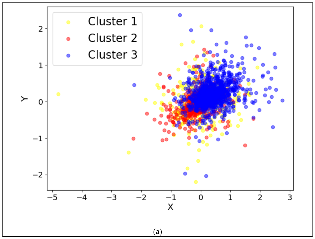
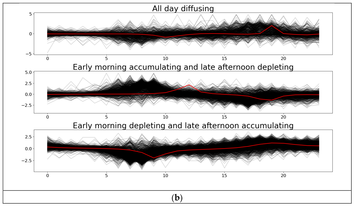
Appendix B. Sensitivity Analysis of PQHR NFR Threshold
Table A1.
Tested parameter settings.
Table A2.
Sensitivity analysis of PQHR weight parameters results. Given PQHR’s sensitivity to the operational-role threshold used to classify provider, receiver, and buffer stations, lower thresholds (0.08–0.09) substantially reduced rebalancing performance because more stations were classified as requiring interventions, thereby reducing the algorithm’s ability to prioritize the most critical stations. By contrast, thresholds between 0.1 and 0.12 produced nearly identical performance. This indicates that PQHR is robust to moderate changes in this parameter. We set the NFR threshold to be 0.1 throughout this study.
Appendix C. Soft-DTW Clustering of Weekday Station Daily NFR Timeseries
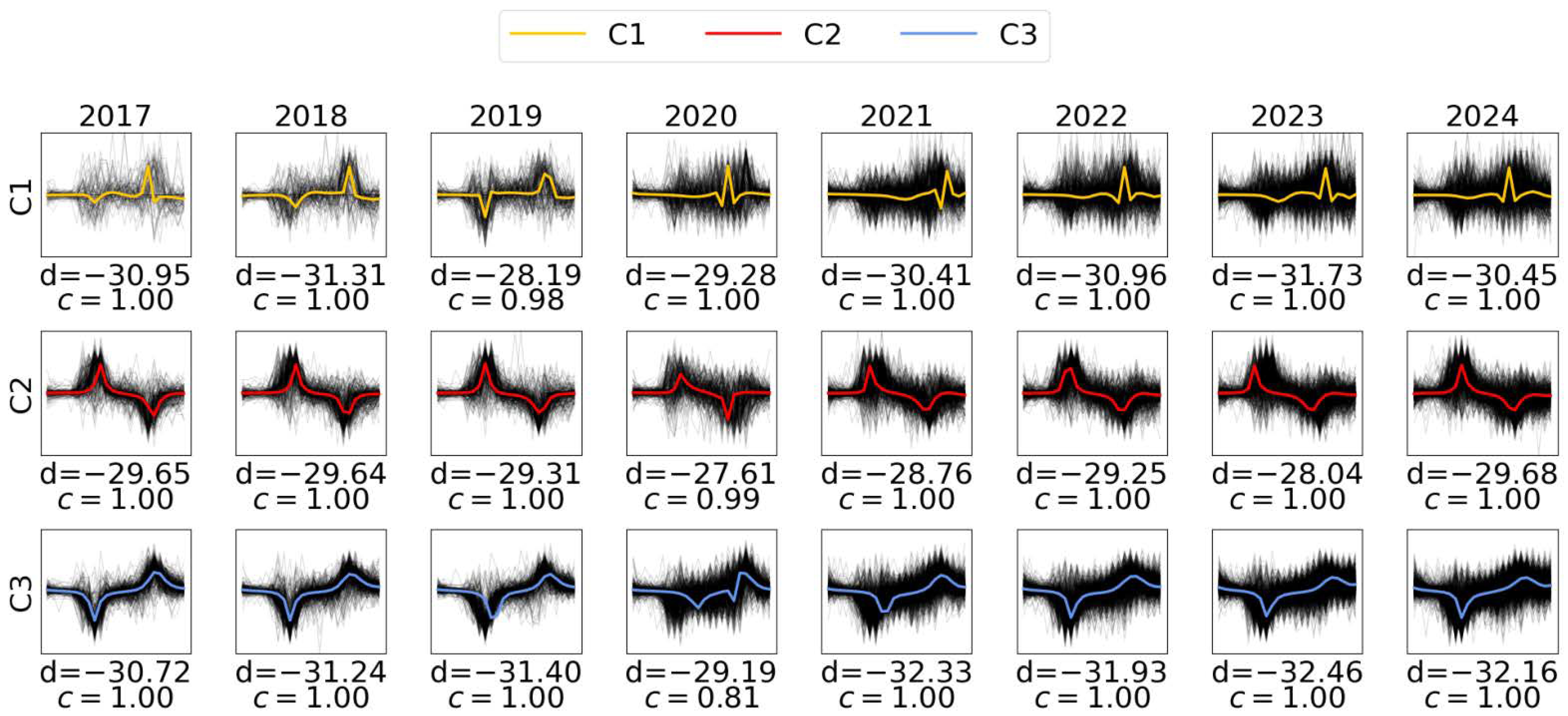
Appendix D. Soft-DTW Clustering of Weekend Station Daily NFR Timeseries
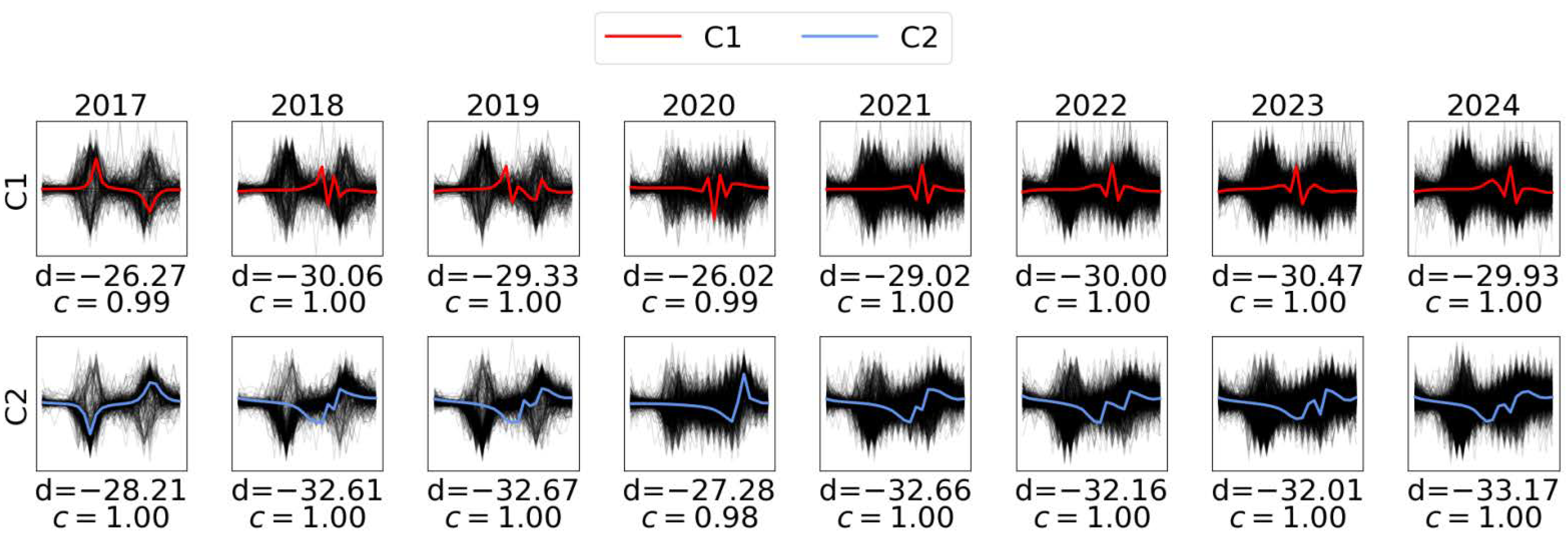
Appendix E. Station Cluster Progression over the Study Period on Weekdays and Weekends
Figure A2.
The 2017–2024 station clustering progression maps illustrate that Citi Bike stations consistently underwent an expansion plan. The clustering of individual stations remains stable over the years, and the most common stations were clustered as “early morning depleting and late afternoon accumulating”, or predominantly near residential areas.
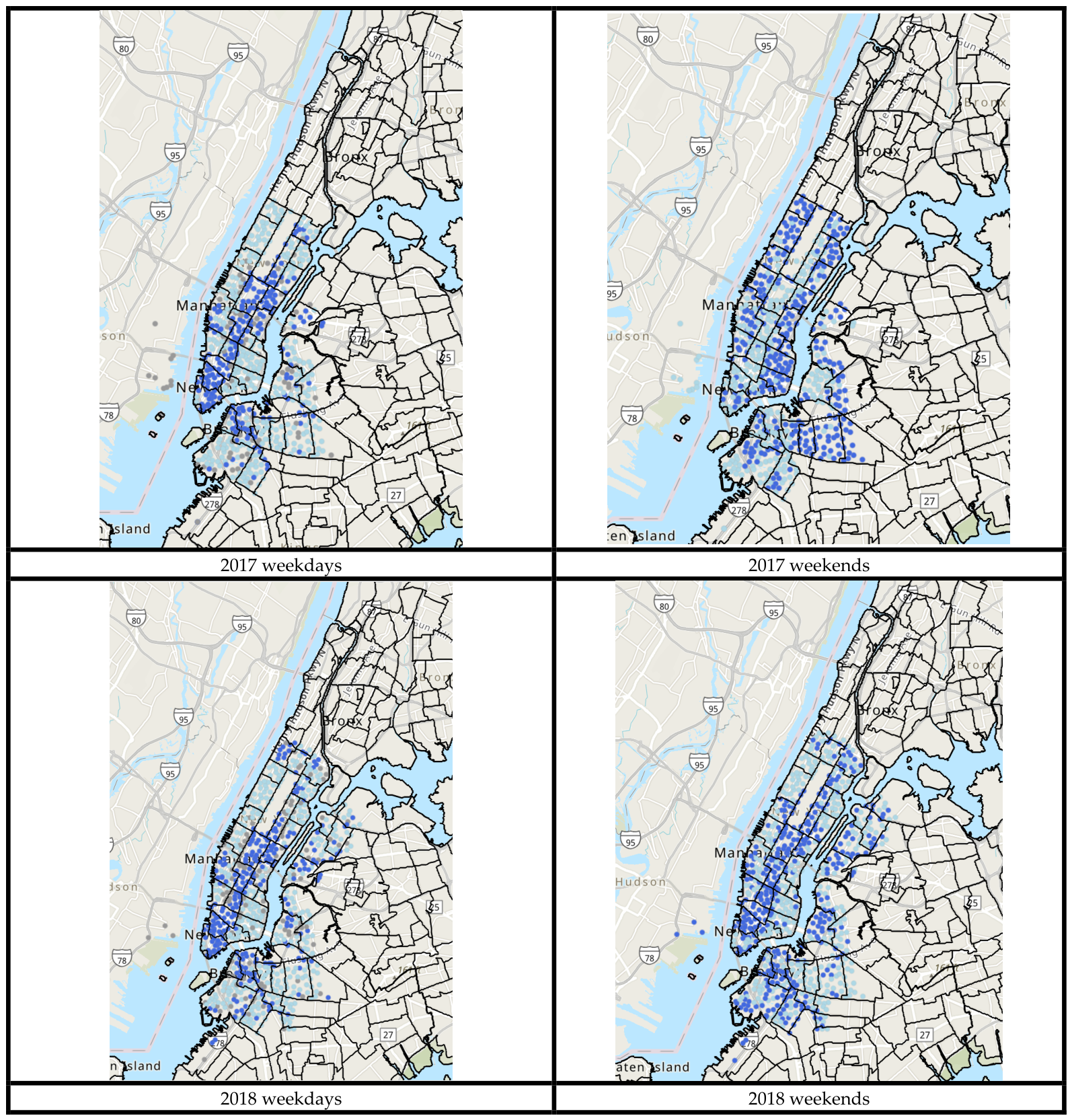
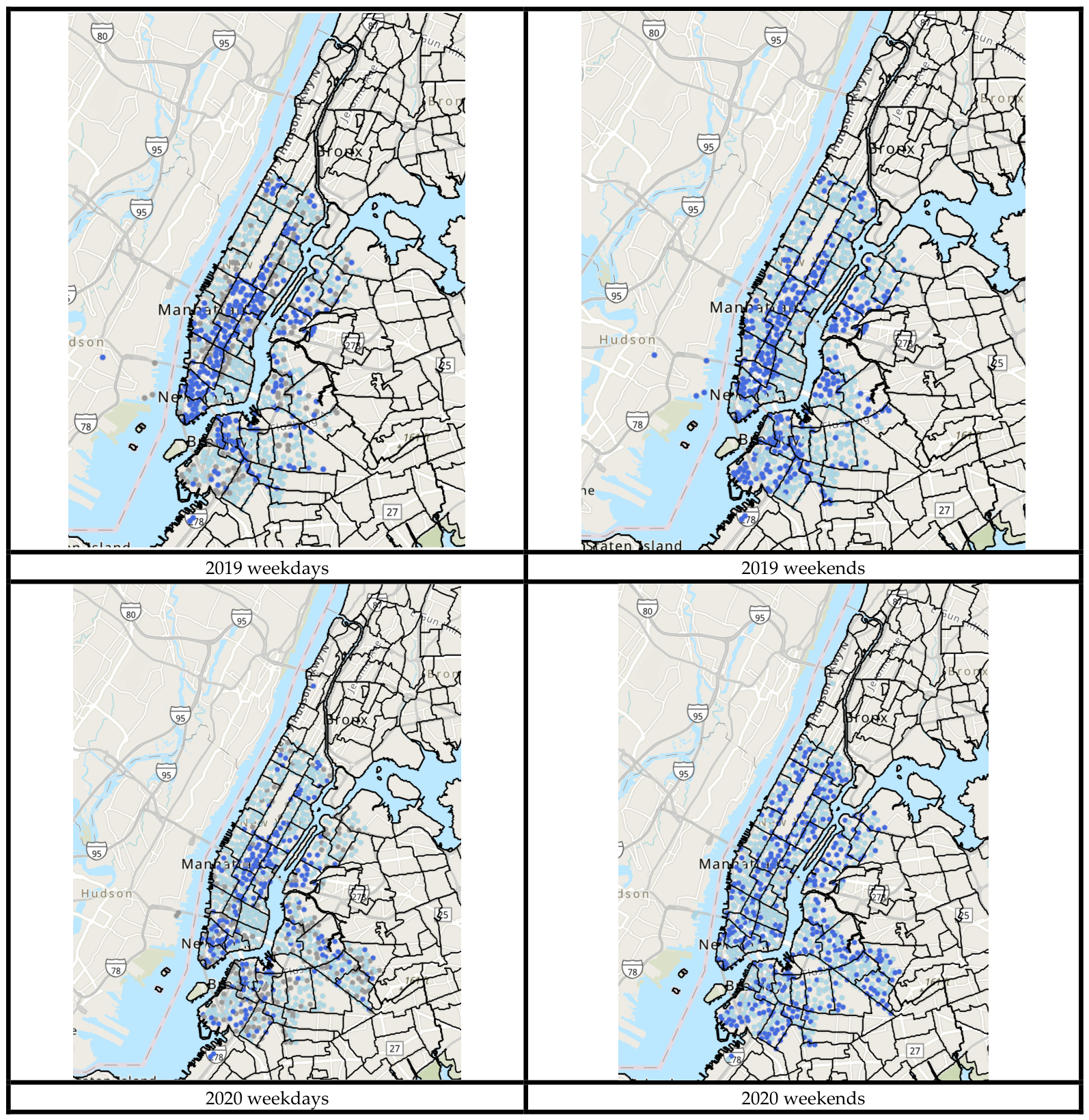
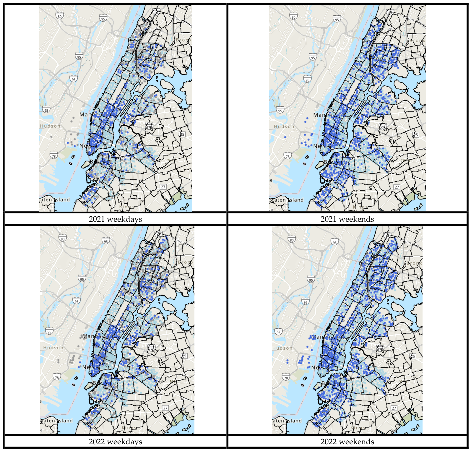
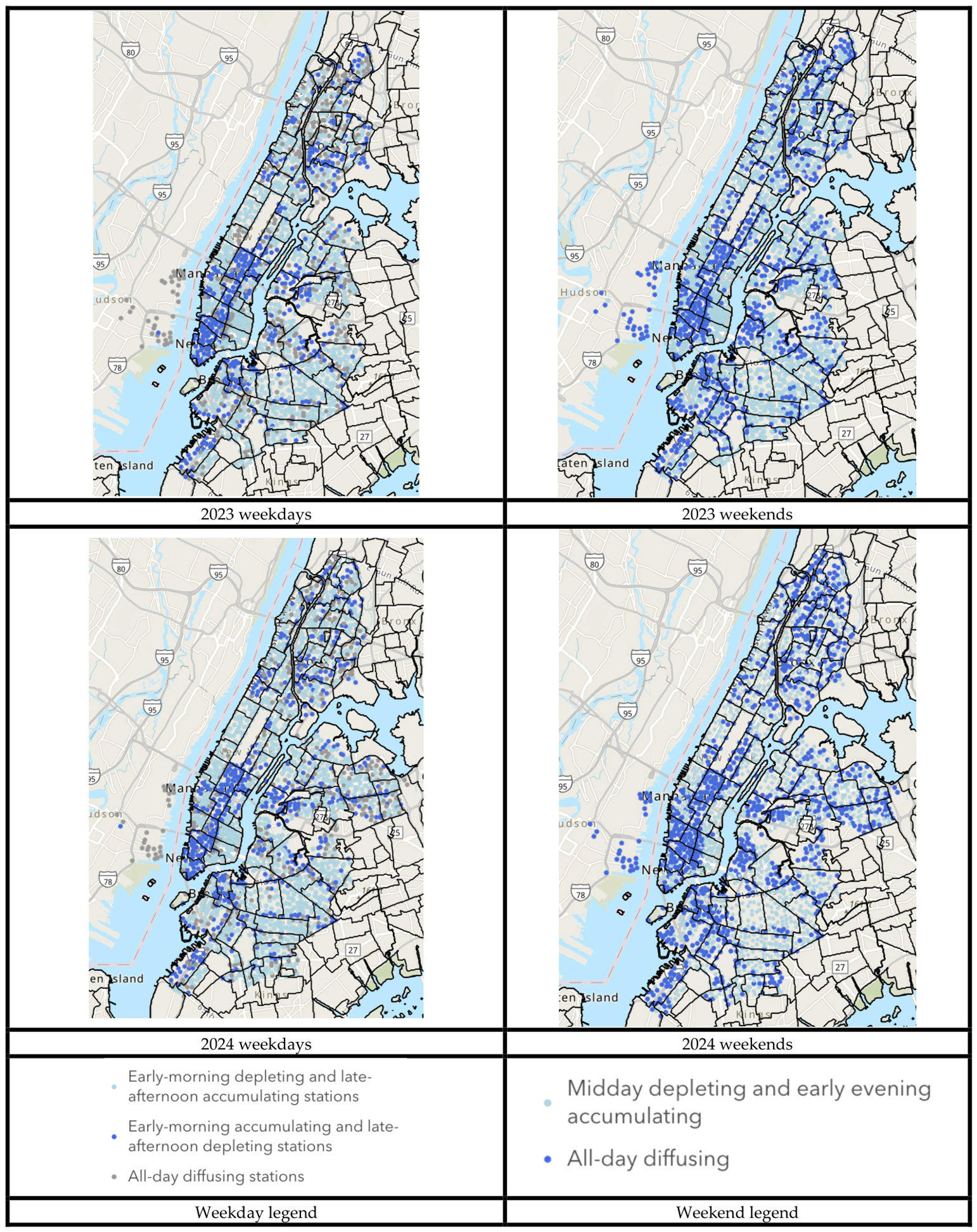
Appendix F. Sensitivity Analysis of PQHR Weight Parameters
Table A3.
Tested parameter settings.
Table A4.
Sensitivity analysis of PQHR weight parameters results. Sensitivity tests showed that PQHR was relatively insensitive to moderate changes in the weighting parameters. Weight schemes ranging from +/−10 to +/−30 produced nearly identical routing performance and similar rebalancing routes. These results indicate that the algorithm is robust rather than finely tuned to a single parameter setting. Only the aggressive weight configuration (+/50%/−30%) for stability and alignment weights, respectively, substantially degraded performance by overemphasizing regime information and reducing route feasibility. Therefore, we set the moderate weighting scheme combinations (+/−20%/+−10%) as our final configuration.
References
- Bike Sharing Market Overview. Available online: https://www.fortunebusinessinsights.com/bike-sharing-market-105908 (accessed on 31 December 2025).
- Musa, S. Insights from a Decade of North American Shared Micromobility Innovation. Available online: https://zagdaily.com/featured/insights-from-a-decade-of-north-american-shared-micromobility-innovation/ (accessed on 31 December 2025).
- Tedeschi, A. Rebalancing Citi Bike: A Geospatial Analysis of Bike Share Redistribution in New York City. Master’s Thesis, Westfälische Wilhelms-Universität Münster (WWU), Münster, Germany, 2016. Available online: https://www.academia.edu/22471385/Rebalancing_Citi_Bike_Mapping_bike_share_redistribution_in_New_York_City (accessed on 31 December 2025).
- Bike Angels. Available online: https://citibikenyc.com/bike-angels (accessed on 31 December 2025).
- Goutam, R.; Goudreault, J.; Pamidimukkala, S. NYC Data Science Academy Data Science Blog Big Data. Data-Driven Predict. Citi Bike Trip Demand. 2022. Available online: https://nycdatascience.com/blog/student-works/predicting-citi-bike-trip-demand/ (accessed on 31 December 2025).
- Scott, S. SeaNYC. Fall CitiBike Rebalancing 2023. Available online: https://seanyc.substack.com/p/the-fall-of-citibike-rebalancing (accessed on 31 December 2025).
- Sekowska, E. Riding Forward: Overhauling Citi Bike’s Contract for Better, More Equitable Service. Available online: https://comptroller.nyc.gov/reports/riding-forward-overhauling-citi-bikes-contract-for-better-more-equitable-service/ (accessed on 31 December 2025).
- New York City Government. 2023 Report on Bike Share Financial Data; New York City Government: New York, NY, USA, 2025. Available online: https://www.nyc.gov/html/dot/downloads/pdf/2023-report-bike-share-financial-data.pdf (accessed on 31 December 2025).
- Gianaris, M. Statement of Senator Michael Gianaris on the Expansion of CitiBike. Available online: https://www.nysenate.gov/newsroom/press-releases/2018/michael-gianaris/statement-senator-michael-gianaris-expansion-citibike (accessed on 31 December 2025).
- Keeping Communities Moving. Available online: https://motivateco.com/ (accessed on 25 December 2025).
- Citi Bike Historical Trip Data. 2025. Available online: https://citibikenyc.com/system-data (accessed on 31 December 2025).
- O’Mahony, E.; Shmoys, D. Data Analysis and Optimization for (Citi)Bike Sharing. Proc. AAAI Conf. Artif. Intell. 2015, 29, 687–694. [Google Scholar] [CrossRef] [Scilit]
- Schuijbroek, J.; Hampshire, R.C.; Van Hoeve, W.-J. Inventory Rebalancing and Vehicle Routing in Bike Sharing Systems. Eur. J. Oper. Res. 2017, 257, 992–1004. [Google Scholar] [CrossRef] [Scilit]
- Liu, J.; Sun, L.; Chen, W.; Xiong, H. Rebalancing Bike Sharing Systems: A Multi-Source Data Smart Optimization. In Proceedings of the 22nd ACM SIGKDD International Conference on Knowledge Discovery and Data Mining; ACM: San Francisco, CA, USA, 2016; pp. 1005–1014. [Google Scholar] [CrossRef] [Scilit]
- Freund, D.; Norouzi-Fard, A.; Paul, A.; Wang, C.; Henderson, S.G.; Shmoys, D.B. Data-Driven Rebalancing Methods for Bike-Share Systems. In Analytics for the Sharing Economy: Mathematics, Engineering and Business Perspectives; Crisostomi, E., Ghaddar, B., Häusler, F., Naoum-Sawaya, J., Russo, G., Shorten, R., Eds.; Springer International Publishing: Cham, Switzerland, 2020; pp. 255–278. ISBN 978-3-030-35031-4. [Google Scholar] [CrossRef] [Scilit]
- Chiariotti, F.; Pielli, C.; Zanella, A.; Zorzi, M. A Dynamic Approach to Rebalancing Bike-Sharing Systems. Sensors 2018, 18, 512. [Google Scholar] [CrossRef] [Scilit] [PubMed]
- Chiariotti, F.; Pielli, C.; Zanella, A.; Zorzi, M. A Bike-Sharing Optimization Framework Combining Dynamic Rebalancing and User Incentives. ACM Trans. Auton. Adapt. Syst. 2019, 14, 1–30. [Google Scholar] [CrossRef] [Scilit]
- Sun, J.; He, Y.; Zhang, J. A Cluster-Then-Route Framework for Bike Rebalancing in Free-Floating Bike-Sharing Systems. Sustainability 2023, 15, 15994. [Google Scholar] [CrossRef] [Scilit]
- O’Brien, O.; Cheshire, J.; Batty, M. Mining Bicycle Sharing Data for Generating Insights into Sustainable Transport Systems. J. Transp. Geogr. 2014, 34, 262–273. [Google Scholar] [CrossRef] [Scilit]
- Faghih-Imani, A.; Eluru, N. Incorporating the Impact of Spatio-Temporal Interactions on Bicycle Sharing System Demand: A Case Study of New York CitiBike System. J. Transp. Geogr. 2016, 54, 218–227. [Google Scholar] [CrossRef] [Scilit]
- Wen, Z.; Tian, D.; Wu, N. Modeling and Analyzing the Spatiotemporal Travel Patterns of Bike Sharing: A Case Study of Citi Bike in New York. Sustainability 2024, 17, 14. [Google Scholar] [CrossRef] [Scilit]
- Choy, D. NYC Data Science Academy Data Science Blog Big Data. Data Analysis on the Distribution of CitiBikes in NYC. 2021. Available online: https://nycdatascience.com/blog/student-works/data-analysis-on-the-distribution-of-citibikes-in-nyc/ (accessed on 31 December 2025).
- An, R.; Zahnow, R.; Pojani, D.; Corcoran, J. Weather and Cycling in New York: The Case of Citibike. J. Transp. Geogr. 2019, 77, 97–112. [Google Scholar] [CrossRef] [Scilit]
- Citi Bike Real-Time Availability. Available online: https://citi-bike-availability.netlify.app/ (accessed on 25 December 2025).
- Citibike Sample Data. Available online: https://citibike-one.vercel.app/ (accessed on 25 December 2025).
- Reilly, K.H.; Wang, S.M.; Gould, L.H.; Baquero, M.; Crossa, A. Characteristics of the Social Network of Bike Share Members in New York City. J. Transp. Health 2021, 22, 101128. [Google Scholar] [CrossRef] [Scilit]
- Hamad, S.Y.Y.; Ma, T.; Antoniou, C. Analysis and Prediction of Bikesharing Traffic Flow—Citi Bike, New York. In Proceedings of the 2021 7th International Conference on Models and Technologies for Intelligent Transportation Systems (MT-ITS); IEEE: Heraklion, Greece, 2021; pp. 1–8. [Google Scholar] [CrossRef] [Scilit]
- Yang, C.; Li, X. Data Mining and Visualization Analysis of Shared Bikes—In the Case of Citi Bike. In Proceedings of the 2018 International Conference on Economics, Business, Management and Corporate Social Responsibility (EBMCSR 2018); Atlantis Press: Zhuhai, China, 2018. [Google Scholar] [CrossRef] [Scilit]
- Saldarriaga, J.F. Columbia Center for Spatial Research Advanced Data Visualization. CitiBike Rebalancing Study An Investigation into Ways to Rebalance CitiBike Stations Throughout New York City. 2013. Available online: https://c4sr.columbia.edu/projects/citibike-rebalancing-study (accessed on 25 December 2025).
- Oliveira, G.N.; Sotomayor, J.L.; Torchelsen, R.P.; Silva, C.T.; Comba, J.L.D. Visual Analysis of Bike-Sharing Systems. Comput. Graph. 2016, 60, 119–129. [Google Scholar] [CrossRef] [Scilit]
- Wiseman, Y. Intelligent Transportation Systems along with the COVID-19 Pandemic Will Significantly Change the Transportation Market. Open Transp. J. 2021, 15, 11–15. [Google Scholar] [CrossRef] [Scilit]
- Lei, Y.; Ozbay, K. A Robust Analysis of the Impacts of the Stay-at-Home Policy on Taxi and Citi Bike Usage: A Case Study of Manhattan. Transp. Policy 2021, 110, 487–498. [Google Scholar] [CrossRef] [Scilit]
- Teixeira, J.F.; Lopes, M. The Link between Bike Sharing and Subway Use during the COVID-19 Pandemic: The Case-Study of New York’s Citi Bike. Transp. Res. Interdiscip. Perspect. 2020, 6, 100166. [Google Scholar] [CrossRef] [Scilit] [PubMed]
- Martí, P.; Serrano-Estrada, L.; Nolasco-Cirugeda, A.; Baeza, J.L. Revisiting the Spatial Definition of Neighborhood Boundaries: Functional Clusters versus Administrative Neighborhoods. J. Urban Technol. 2022, 29, 73–94. [Google Scholar] [CrossRef] [Scilit]
- Zook, M.A.; Graham, M. Mapping DigiPlace: Geocoded Internet Data and the Representation of Place. Environ. Plan. B Plan. Des. 2007, 34, 466–482. [Google Scholar] [CrossRef] [Scilit]
- Atwal, K.S.; Anderson, T.; Pfoser, D.; Züfle, A. Predicting Building Types Using OpenStreetMap. Sci. Rep. 2022, 12, 19976. [Google Scholar] [CrossRef] [Scilit] [PubMed]
- Satman, M.H.; Altunbey, M. Selecting Location of Retail Stores Using Artificial Neural Networks and Google Places API. Int. J. Stat. Probab. 2014, 3, p67. [Google Scholar] [CrossRef] [Scilit]
- Rigobon, D.E.; Duprey, T.; Kotlicki, A.; Schnattinger, P.; Baharian, S.; Hurd, T.R. Business Closures and (Re)Openings in Real-Time Using Google Places: Proof of Concept. J. Risk Financ. Manag. 2022, 15, 183. [Google Scholar] [CrossRef] [Scilit]
- Gubert, F.R.; Santos, G.H.; Delgado, M.; Silver, D.; Silva, T.H. Urban Cultural Signature with Web Data: A Case Study with Google Places Venues. J. Internet Serv. Appl. 2025, 16, 388–406. [Google Scholar] [CrossRef] [Scilit]
- Tavenard, R.; Faouzi, J.; Vandewiele, G.; Divo, F.; Androz, G.; Holtz, C.; Payne, M.; Yurchak, R.; Rußwurm, M.; Kolar, K.; et al. Tslearn, A Machine Learning Toolkit for Time Series Data. J. Mach. Learn. Res. 2020, 21, 1–6. Available online: https://jmlr.org/papers/v21/20-091.html (accessed on 25 December 2025).
- Zakaria, J.; Mueen, A.; Keogh, E. Clustering Time Series Using Unsupervised-Shapelets. In Proceedings of the 2012 IEEE 12th International Conference on Data Mining; IEEE: Brussels, Belgium, 2012; pp. 785–794. Available online: https://www.semanticscholar.org/paper/Clustering-Time-Series-Using-Unsupervised-Shapelets-Zakaria-Mueen/c271f40ed89655845a9d591fa8ae7cefbd9a92e1 (accessed on 25 December 2025).
- Kobylin, O.; Lyashenko, V. Time Series Clustering Based on the K-Means Algorithm. J. Multiapp 2020, 1, 1–7. [Google Scholar] [CrossRef] [Scilit]
- Senin, P. Dynamic Time Warping Algorithm Review. 2008. Available online: https://seninp.github.io/assets/pubs/senin_dtw_litreview_2008.pdf (accessed on 25 December 2025).
- Cuturi, M.; Blondel, M. Soft-DTW: A Differentiable Loss Function for Time-Series. arXiv 2017. [Google Scholar] [CrossRef] [Scilit]
- Paparrizos, J.; Gravano, L. K-Shape: Efficient and Accurate Clustering of Time Series. ACM SIGMOD Rec. 2016, 45, 69–76. [Google Scholar] [CrossRef] [Scilit]
- Shorewala, V.; Shorewala, S. Anomaly Detection and Improvement of Clusters Using Enhanced K-Means Algorithm. arXiv 2025. [Google Scholar] [CrossRef] [Scilit]
- Dhillon, I.S.; Guan, Y.; Kulis, B. Kernel K-Means: Spectral Clustering and Normalized Cuts. In Proceedings of the Tenth ACM SIGKDD International Conference on Knowledge Discovery and Data Mining; ACM: Seattle, WA, USA, 2004; pp. 551–556. [Google Scholar] [CrossRef] [Scilit]
- Lei, Q.; Yi, J.; Vaculin, R.; Wu, L.; Dhillon, I.S. Similarity Preserving Representation Learning for Time Series Clustering. 2017. Available online: https://dl.acm.org/doi/abs/10.5555/3367243.3367434 (accessed on 25 December 2025).
- Dijkstra, E.W. A Note on Two Problems in Connexion with Graphs. Numer. Math. 1959, 1, 269–271. [Google Scholar] [CrossRef] [Scilit]
- Gavish, B.; Graves, S.C. The Travelling Salesman Problem and Related Problems; Massachusetts Institute of Technology Operations Research Center: Cambridge, MA, USA, 1978. [Google Scholar]
- Zeng, Z.; Veeravalli, B. Design and Performance Evaluation of Queue-and-Rate-Adjustment Dynamic Load Balancing Policies for Distributed Networks. IEEE Trans. Comput. 2006, 55, 1410–1422. [Google Scholar] [CrossRef] [Scilit]
- Ambigavathi, M.; Sridharan, D. Energy Efficient and Load Balanced Priority Queue Algorithm for Wireless Body Area Network. Future Gener. Comput. Syst. 2018, 88, 586–593. [Google Scholar] [CrossRef] [Scilit]
- Hu, R.; Zhang, Z.; Ma, X.; Jin, Y. Dynamic Rebalancing Optimization for Bike-Sharing System Using Priority-Based MOEA/D Algorithm. IEEE Access 2021, 9, 27067–27084. [Google Scholar] [CrossRef] [Scilit]
- Smith, S.L.; Pavone, M.; Schwager, M.; Frazzoli, E.; Rus, D. Rebalancing the Rebalancers: Optimally Routing Vehicles and Drivers in Mobility-on-Demand Systems. In Proceedings of the 2013 American Control Conference; IEEE: Washington, DC, USA, 2013; pp. 2362–2367. [Google Scholar]
- Duan, Y.; Wu, J.; Zheng, H. A Greedy Approach for Vehicle Routing When Rebalancing Bike Sharing Systems. In Proceedings of the 2018 IEEE Global Communications Conference (GLOBECOM); IEEE: Abu Dhabi, United Arab Emirates, 2018; pp. 1–7. [Google Scholar]
- Kroes, J.R.; Manikas, A.S.; Gattiker, T.F. Generating Efficient Rebalancing Routes for Bikeshare Programs Using a Genetic Algorithm. J. Clean. Prod. 2020, 244, 118880. [Google Scholar] [CrossRef] [Scilit]
- Yu, Q.; Gu, Y.; Yang, S.; Zhou, M. Discovering Spatiotemporal Patterns and Urban Facilities Determinants of Cycling Activities in Beijing. J. Geovisualization Spat. Anal. 2021, 5, 16. [Google Scholar] [CrossRef] [Scilit]
- Citi Bike Station Information. 2025. Available online: https://gbfs.citibikenyc.com/gbfs/en/station_information.json (accessed on 25 December 2025).
- Citi Bike Real-Time Data. 2025. Available online: https://gbfs.citibikenyc.com/gbfs/en/station_status.json (accessed on 31 December 2025).
- Governor Cuomo Signs the “New York State on PAUSE” Executive Order. Available online: https://www.governor.ny.gov/news/governor-cuomo-signs-new-york-state-pause-executive-order (accessed on 25 December 2025).
- Tslearn Documentation. Available online: https://tslearn.readthedocs.io/en/stable/ (accessed on 25 December 2025).
- Tavenard, R. Differentiability of DTW and the Case of Soft-DTW. Blog Romain Tavenard. 2021. Available online: https://rtavenar.github.io/blog/softdtw.html (accessed on 25 December 2025).
- Vásconez, J.P.; Schotborgh, E.; Vásconez, I.N.; Moya, V.; Pilco, A.; Menéndez, O.; Guamán-Rivera, R.; Guevara, L. Smart Delivery Assignment through Machine Learning and the Hungarian Algorithm. Smart Cities 2024, 7, 1109–1125. [Google Scholar] [CrossRef] [Scilit]
- GeoPandas. 2026. Available online: https://geopandas.org/en/stable/ (accessed on 25 December 2025).
- ArcGIS Online. 2026. Available online: https://www.arcgis.com/ (accessed on 25 December 2025).
- Neighborhood Tabulation Areas (NTAs). Available online: https://www.nyc.gov/content/planning/pages/resources/datasets/neighborhood-tabulation (accessed on 25 December 2025).
- Python Folium Visualization. 2026. Available online: https://python-visualization.github.io/folium/latest/ (accessed on 15 June 2025).
- Reid, C.E.; Kubzansky, L.D.; Li, J.; Shmool, J.L.; Clougherty, J.E. It’s Not Easy Assessing Greenness: A Comparison of NDVI Datasets and Neighborhood Types and Their Associations with Self-Rated Health in New York City. Health Place 2018, 54, 92–101. [Google Scholar] [CrossRef] [Scilit] [PubMed]
- Liu, J.; Sun, L.; Li, Q.; Ming, J.; Liu, Y.; Xiong, H. Functional Zone Based Hierarchical Demand Prediction For Bike System Expansion. In Proceedings of the 23rd ACM SIGKDD International Conference on Knowledge Discovery and Data Mining; ACM: Halifax, NS, Canada, 2017; pp. 957–966. [Google Scholar] [CrossRef] [Scilit]
- Wang, J.; Huang, J.; Dunford, M. Rethinking the Utility of Public Bicycles: The Development and Challenges of Station-Less Bike Sharing in China. Sustainability 2019, 11, 1539. [Google Scholar] [CrossRef] [Scilit]
- Guo, Y.; Zhou, J.; Wu, Y.; Li, Z. Identifying the Factors Affecting Bike-Sharing Usage and Degree of Satisfaction in Ningbo, China. PLoS ONE 2017, 12, e0185100. [Google Scholar] [CrossRef] [Scilit] [PubMed]
- Zheng, Z.; Chen, Y.; Zhu, D.; Sun, H.; Wu, J.; Pan, X.; Li, D. Extreme Unbalanced Mobility Network in Bike Sharing System. Phys. Stat. Mech. Its Appl. 2021, 563, 125444. [Google Scholar] [CrossRef] [Scilit]
- Du, Y.; Deng, F.; Liao, F. A Model Framework for Discovering the Spatio-Temporal Usage Patterns of Public Free-Floating Bike-Sharing System. Transp. Res. Part C Emerg. Technol. 2019, 103, 39–55. [Google Scholar] [CrossRef] [Scilit]
- McBain, C.; Caulfield, B. An Analysis of the Factors Influencing Journey Time Variation in the Cork Public Bike System. Sustain. Cities Soc. 2018, 42, 641–649. [Google Scholar] [CrossRef] [Scilit]
- New York City’s Zoning & Land Use Map. 2025. Available online: https://zola.planninglabs.nyc/ (accessed on 25 December 2025).
- Census Bureau Reports 1.6 Million Workers Commute into Manhattan Each Day. 2013. Available online: https://www.census.gov/newsroom/archives/2013-pr/cb13-r17.html (accessed on 25 December 2025).
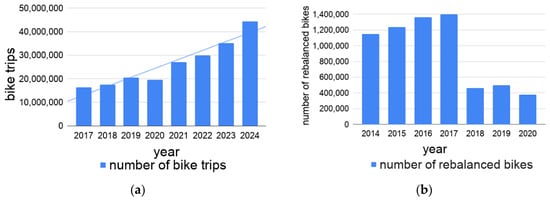
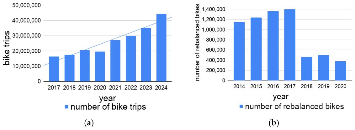
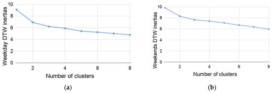
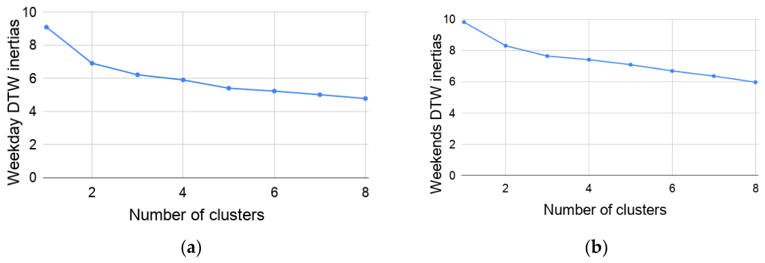
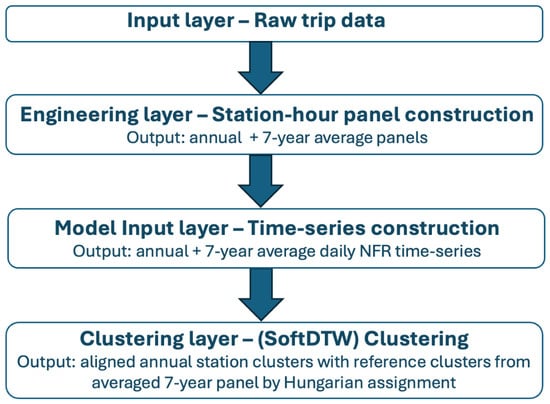
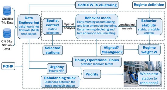
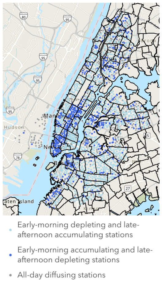
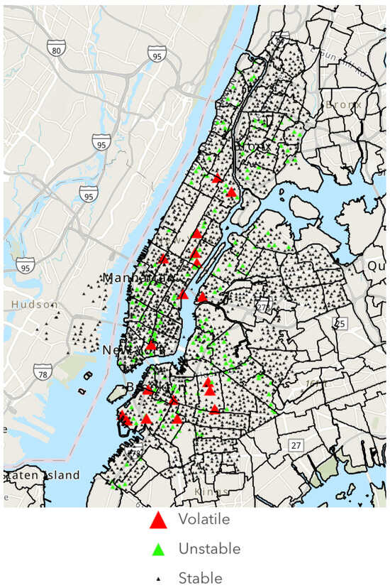
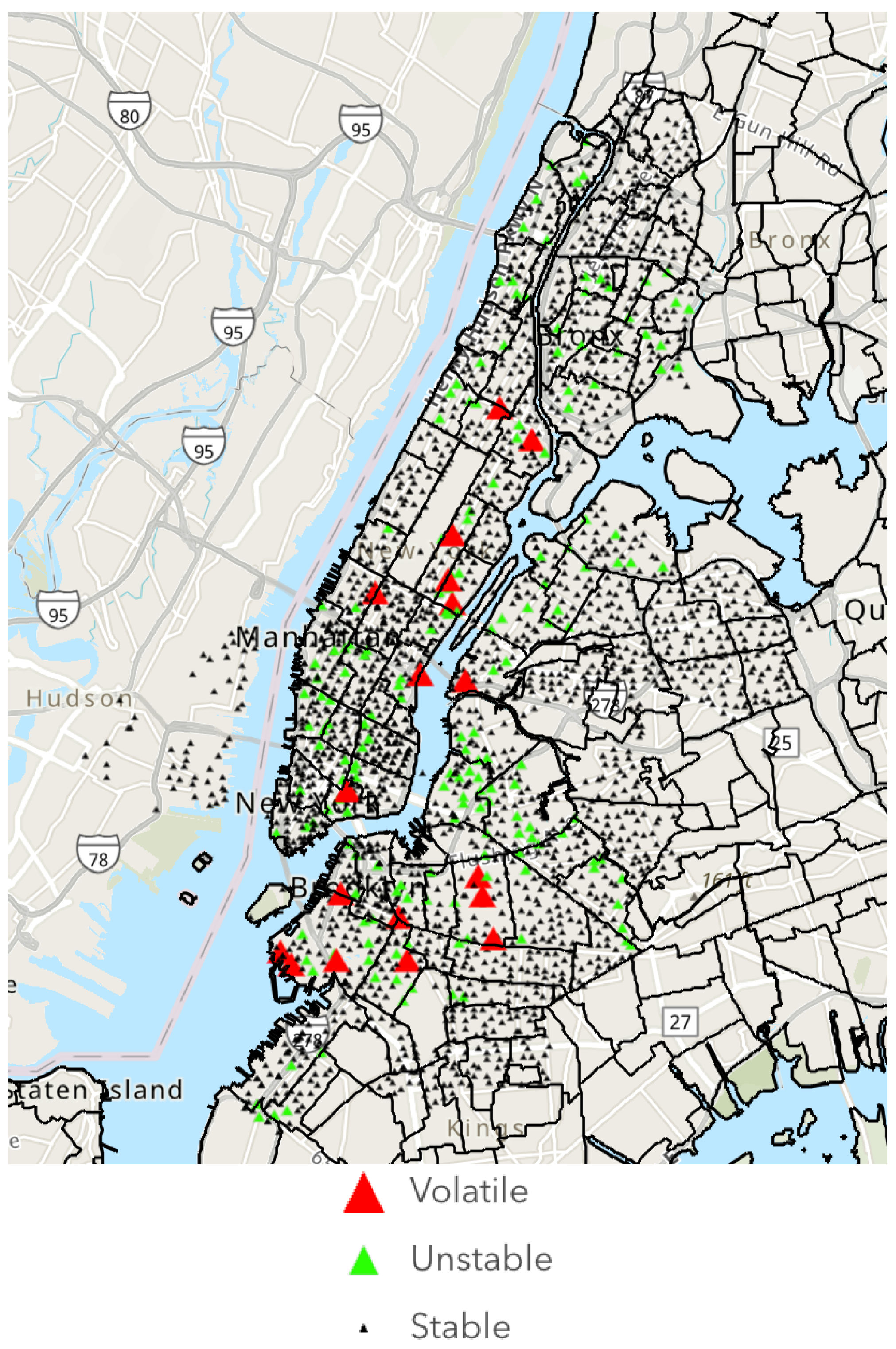
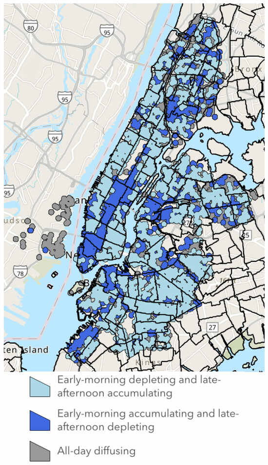
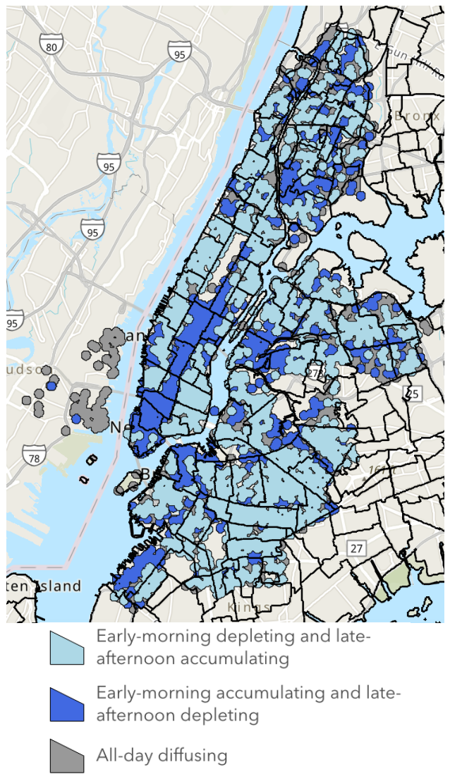
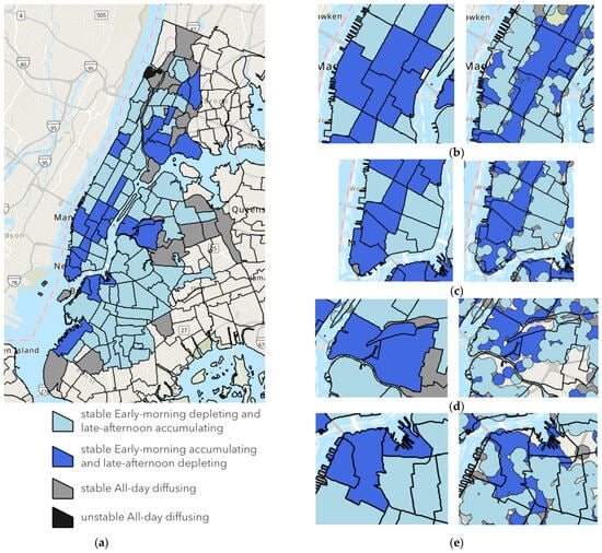
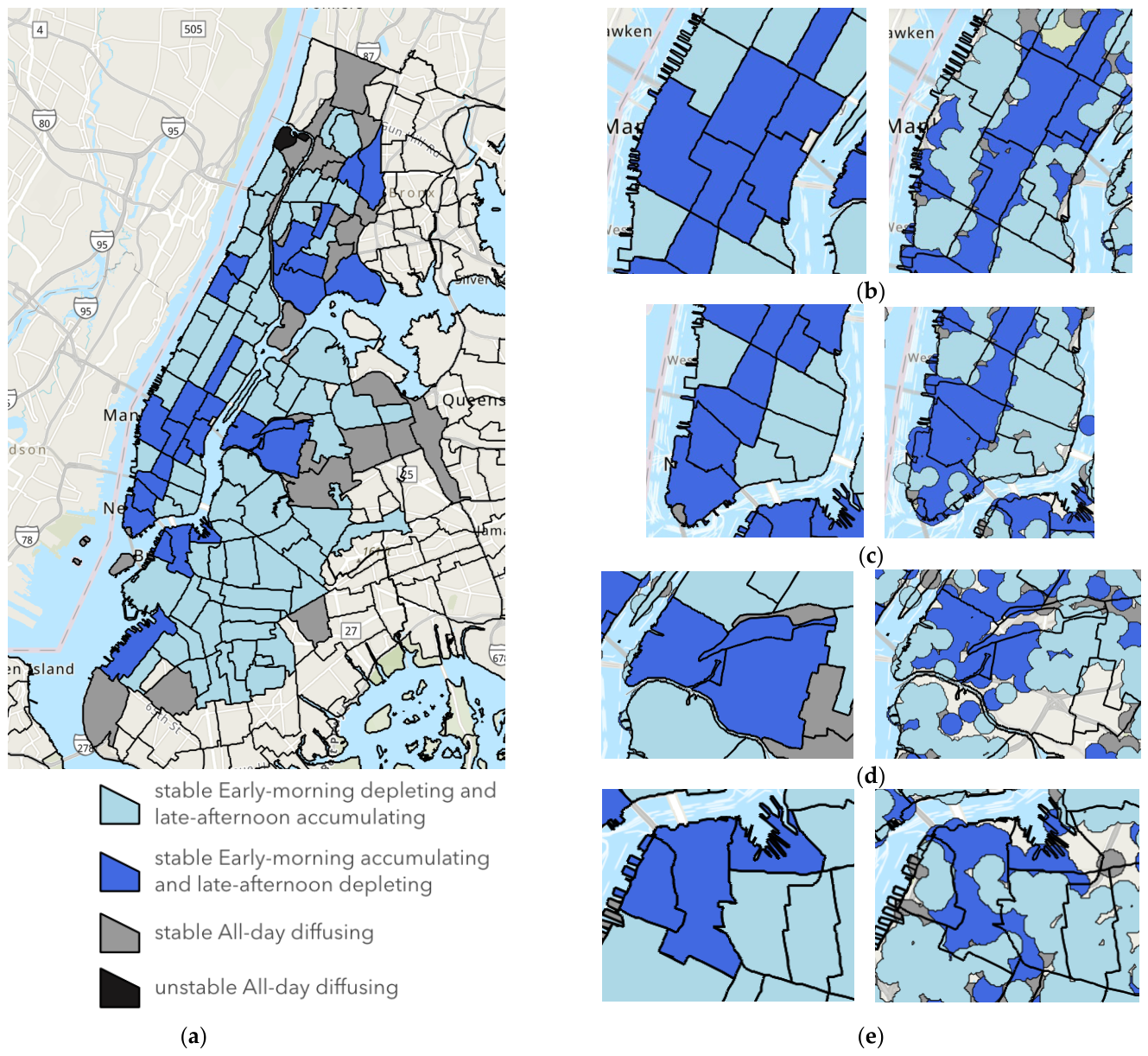
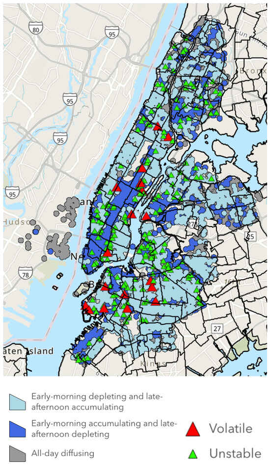
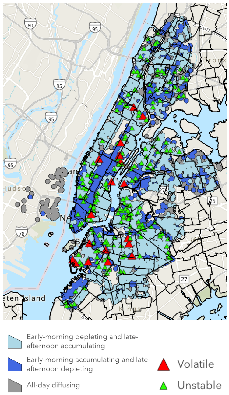
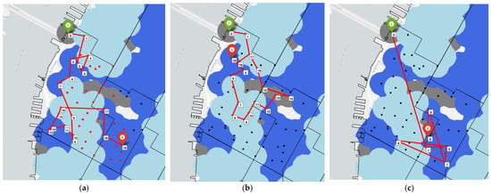
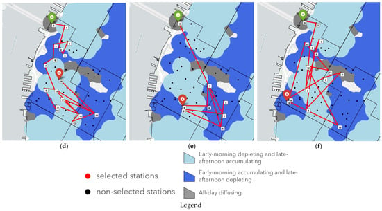
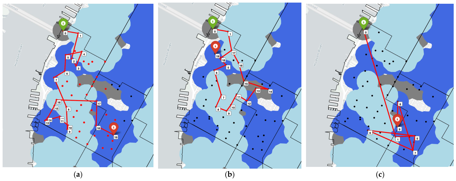
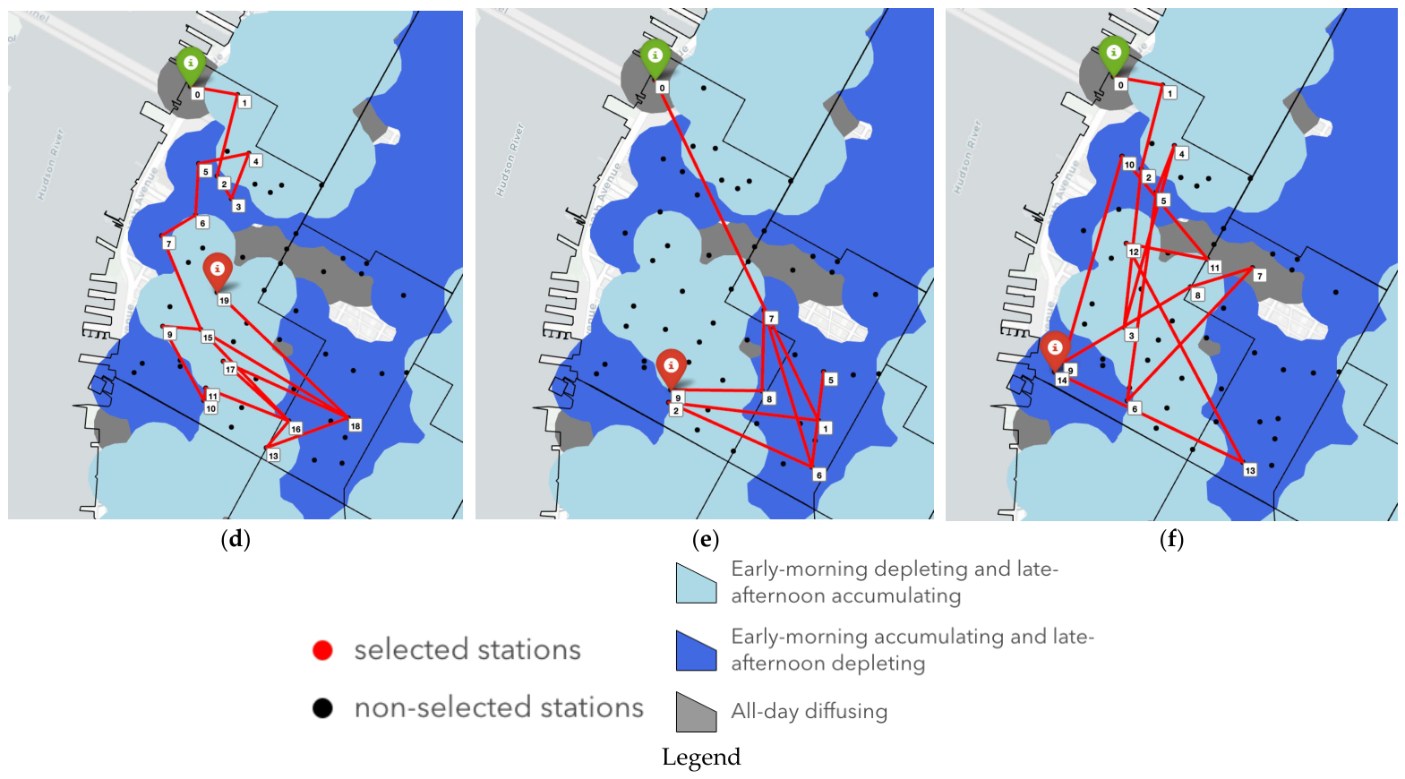
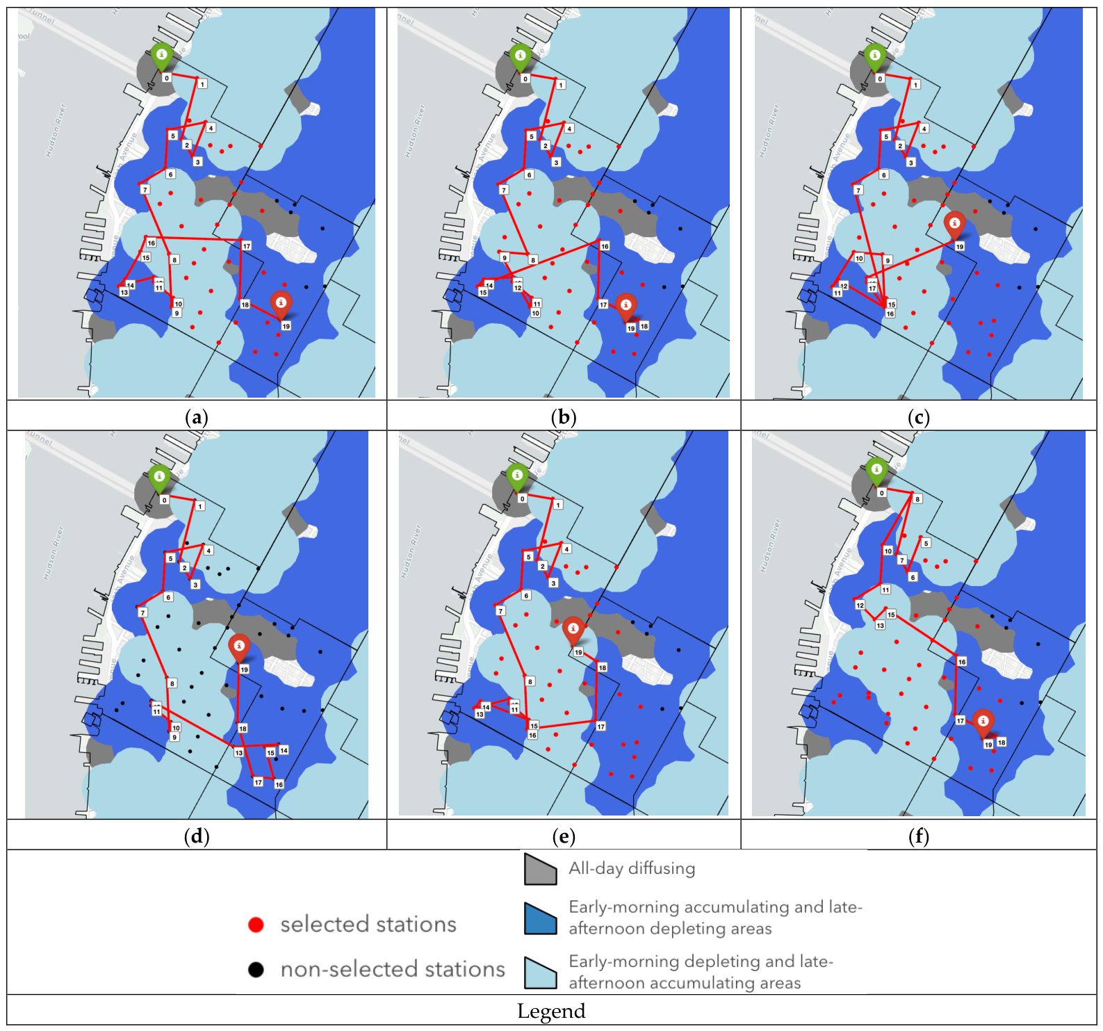

Disclaimer/Publisher’s Note: The statements, opinions and data contained in all publications are solely those of the individual author(s) and contributor(s) and not of MDPI and/or the editor(s). MDPI and/or the editor(s) disclaim responsibility for any injury to people or property resulting from any ideas, methods, instructions or products referred to in the content. |
© 2026 by the author. Licensee MDPI, Basel, Switzerland. This article is an open access article distributed under the terms and conditions of the Creative Commons Attribution (CC BY) license.