A Spatio-Temporal Hybrid Multi-Head Attention Model for AIS-Based Ship Trajectory Prediction

Abstract

To improve ship AIS trajectory prediction under pronounced spatiotemporal coupling and dynamic maneuvering conditions, this study proposes a Spatio-Temporal-Hybrid-Multi-head Attention model (STHA) integrating multiscale convolution, bidirectional long short-term memory, and multi-head attention. Historical AIS data from the Zhoushan waters in 2024 were preprocessed through screening, cleaning, outlier removal, resampling, and cubic spline interpolation to construct trajectory samples. Comparative experiments were conducted against BP, BiLSTM, and BiGRU using MAPE, RMSE, and R² as evaluation metrics. The results show that STHA achieves the best overall predictive performance, more accurately follows trajectory variations across different vessel types, and exhibits better robustness in scenarios involving turning and speed changes. These findings indicate that the proposed model is effective for high-precision ship trajectory prediction and can provide useful support for subsequent collision risk assessment and navigation safety assistance.

1. Introduction

With the continued expansion of global maritime transport and the steady increase in vessel traffic density in key waters, the frequency of ship encounters has risen significantly, rendering navigational safety issues in complex sailing environments increasingly prominent. As a critical foundation for maritime traffic situational awareness, collision risk assessment, and intelligent navigation assistance, ship trajectory prediction directly affects the effectiveness of subsequent risk identification and maritime regulatory decision-making through its accuracy and stability. In recent years, the widespread application of the Automatic Identification System (AIS) has provided abundant data support for modeling vessel movement behavior. AIS data can comprehensively record dynamic information during vessel navigation, including position, course, and speed, thereby providing a reliable data basis for mining vessel movement patterns and predicting future trajectories.

Extensive and systematic research has been conducted worldwide on ship trajectory prediction, and the related approaches can generally be categorized into methods based on physical characteristics and statistical theory, machine learning methods, and deep learning methods. In studies grounded in physical characteristics and statistical theory, Perera [1] developed a mathematical model for estimating ship operating states and parameters and validated it through ship maneuvering simulations; Liu Xiaoxuan et al. [2] established a system for long-range grounding risk warning by integrating sensor networks with AIS data to realize future trajectory inference; Tong Xiaopeng et al. [3] predicted ship trajectories by combining a Markov chain and a grey model on the basis of kinematic equations; Luo et al. [4] performed trajectory inference using a vector analysis method, whereas Li Rao et al. [5] established a physical prediction model based on inertial navigation principles. In addition, Martelli et al. [6] developed a decision-support tool that integrates AIS data with ship collision-avoidance regulations, and Hu et al. [7] further examined the role of COLREGs in ship navigation and dynamic route adjustment. With respect to statistical-theory-based methods, future trends are primarily inferred by mining the time-series characteristics of historical trajectories. Representative approaches include the Markov model [8], time-series analysis [9], Kalman filtering [10], and trajectory similarity matching [11]. Although such methods possess strong interpretability in terms of mechanism, they often rely on strong prior assumptions and remain limited in their adaptability to complex nonlinear navigation scenarios. As the scale of AIS data has continued to grow, researchers have increasingly adopted data-driven machine learning methods for ship trajectory prediction. Chen et al. [12] introduced sparse Gaussian process regression into the trajectory prediction task, although its performance remained highly dependent on input data quality; Rong et al. [13] proposed a framework integrating regression models with Gaussian process regression to jointly predict ship destinations and trajectories; Borkowski et al. [14] employed a generalized regression neural network to enhance the robustness and real-time performance of trajectory fitting; Gan et al. [15] combined K-means clustering with an artificial neural network and incorporated multidimensional features such as ship speed, load, and power for trajectory prediction; Yang et al. [16] used DBSCAN for trajectory clustering analysis, thereby providing effective data preprocessing support for subsequent prediction models. In addition, single-point neighbor search methods [17], particle swarm optimization algorithms [18], and random forest methods [19,20,21] have been widely applied to related tasks such as ship behavior prediction, turning-angle prediction, arrival-time prediction, destination-port identification, and speed estimation. Overall, machine learning methods outperform traditional analytical models in scenario adaptability and modeling flexibility, but they remain highly dependent on feature engineering and data quality and are still limited in the automatic representation of complex spatiotemporal correlations. In recent years, deep learning has gradually become a major research direction in ship trajectory prediction because of its advantages in learning complex nonlinear mappings and high-dimensional spatiotemporal features. Chen Dakai et al. [22] developed a ship trajectory prediction model based on a long short-term memory (LSTM) network, using longitude, latitude, speed, and course from AIS data as inputs to achieve real-time inference of ship navigation trajectories. On this basis, Liu et al. [23] introduced an attention mechanism into the LSTM model, effectively alleviating data distortion and spatiotemporal discontinuity; Murray et al. [24] designed a bilinear autoencoder to estimate the latent distribution of trajectories and quantify positional uncertainty; Li et al. [25] constructed an LSTM encoder-decoder architecture, which demonstrated superior performance over traditional statistical methods in traffic flow modeling tasks. To capture bidirectional temporal dependencies more comprehensively, researchers subsequently proposed various improved methods based on bidirectional long short-term memory (BiLSTM), such as prediction models incorporating data denoising techniques, improved methods combined with spectral clustering, novel architectures integrating attention mechanisms, and bidirectional recurrent neural network variants [26], improved methods combined with spectral clustering [27], novel architectures integrating attention mechanisms [28], and BiLSTM recurrent neural networks [29]. Meanwhile, to improve model complexity and training efficiency, substantial research has also been conducted on gated recurrent unit (GRU)-based methods. Suo et al. [30] designed a prediction method integrating GRU with a trajectory correction algorithm, thereby improving computational efficiency while maintaining high accuracy; Zhang et al. [31] constructed a GRU–multiscale convolutional neural network architecture and integrated an autoregressive model to fully exploit spatiotemporal features; Wang et al. [32] proposed a bidirectional GRU model that outperformed traditional RNNs; Chen et al. [33] designed a forward-backward bidirectional GRU architecture and optimized the trajectory fitting process through a bidirectional scaling mechanism. Although these studies have significantly improved the performance of ship trajectory prediction, further optimization is still needed with respect to fluctuating AIS data quality, local spatial pattern recognition, long-sequence dependency modeling, and stable prediction under complex maneuvering scenarios.

In summary, although existing studies on ship trajectory prediction have made substantial progress, several key challenges remain. On the one hand, AIS trajectory data often contain missing values, noise, drifting points, and irregular sampling intervals, which reduce sample quality and may weaken model generalization. On the other hand, ship AIS trajectory sequences exhibit pronounced spatiotemporal coupling characteristics, because longitude, latitude, speed, and course evolve jointly over time, and spatial movement patterns are closely interrelated with temporal dependencies. As a result, ship trajectories involve both local spatial variation patterns and longer-range temporal dependencies, while many existing methods still struggle to capture these two aspects simultaneously. Traditional physical and statistical methods generally rely on strong prior assumptions and are less adaptable to nonlinear navigation scenarios. Conventional machine learning methods provide improved flexibility but remain strongly dependent on feature engineering and data quality. Deep learning models based on recurrent structures enhance temporal modeling capability, yet they may still be insufficient for capturing multiscale local spatial patterns and may exhibit error accumulation or tail-end drift in dynamic maneuvering scenarios involving turning and speed changes. To address these limitations, this study proposes a ship trajectory prediction model termed STHA (Spatio-Temporal Hybrid Multi-Head Attention). First, systematic preprocessing is applied to reduce the influence of missing values, noise, drifting points, and irregular sampling intervals in raw AIS data. Second, a multiscale convolutional module is used to capture local trajectory variation patterns under different receptive fields. Third, BiLSTM is employed to model temporal dependencies across the input sequence. Finally, a multi-head attention mechanism is introduced to emphasize critical historical states that contribute more substantially to the current prediction. Experimental results demonstrate that the proposed model achieves favorable accuracy and generalization ability in trajectory prediction tasks. Compared with benchmark models such as Back Propagation Neural Network (BP), BiLSTM, and BiGRU, it exhibits lower error levels, greater robustness to fluctuations, and better tail-end stability in dynamic maneuvering scenarios involving turning and speed changes. The remainder of this paper is organized as follows. Section 2 introduces the AIS data source, data preprocessing methods, and the formulation of the trajectory prediction problem. Section 3 presents the experimental design, evaluation metrics, comparative experimental settings, and prediction results. Section 4 discusses the results, summarizes the main findings, and outlines directions for future research.

2. Materials and Methods

2.1. Data Sources and Preprocessing

2.1.1. Data Sources

The Automatic Identification System (AIS) data used in this study were obtained from the annual historical AIS dataset for the Zhejiang waters in 2024, which was purchased by a university research group specializing in navigation. The original data were provided by Shipxy (Beijing, China) and subsequently organized by EhaiLan Co., Ltd. (Beijing, China). AIS data can continuously record dynamic information during vessel navigation and thus constitute an important foundation for ship trajectory prediction research.

Given that the focus of this study is on vessel movement patterns in waters adjacent to typical ports, the study area was limited to the offshore waters of Zhoushan. The geographic boundaries of the target waters were defined as 121°21′0″–123°48′0″ longitude and 30°4′12″–30°19′48″ latitude. To ensure the representativeness of the temporal distribution of samples, AIS data from the 5th, 15th, and 25th day of each month from January to December 2024 were selected for analysis, on the basis of which the experimental samples were constructed. After data preprocessing, historical trajectory data for 2685 vessels in the study area were ultimately obtained, covering multiple vessel types, including cargo ships, passenger ships, container ships, fishing vessels, and oil tankers, thereby providing reliable data support for the subsequent training and testing of the trajectory prediction model.

2.1.2. Data Preprocessing

To ensure the continuity, smoothness, and physical plausibility of the training samples for the subsequent trajectory prediction model, the raw AIS data were systematically preprocessed before modeling. The preprocessing procedure mainly consisted of three steps: data screening and cleaning, outlier identification and removal, and trajectory resampling and interpolation-based completion. Since AIS data generally contain invalid values, missing values, abnormal positions, drifting points, and uneven sampling intervals during acquisition and transmission, data quality control had to be completed before model training.

• Data Screening and Cleaning:

First, the raw AIS data were screened according to the study area and time range, and only records within the target waters and study period were retained. In accordance with the modeling requirements, only the core fields, including Maritime Mobile Service Identity (MMSI), DateTime, latitude (LAT), longitude (LON), Speed Over Ground (SOG), Course Over Ground (COG), and ship type, were extracted, while irrelevant attributes were removed and the remaining fields were reordered. Subsequently, records that clearly violated physical plausibility were cleaned, including those with missing MMSI values, zero longitude or latitude, negative speed, or abnormal course values. Records with missing values in key fields such as time, position, and speed were also directly removed. Through these procedures, the interference of anomalous messages and invalid information with subsequent trajectory modeling could be effectively reduced.

2.

Outlier Identification and Removal:

To address unreasonable paths that may occur in AIS trajectories, such as long-distance jumps, crossings over islands, or extensions into inland areas, a method combining geographic distance mutation and speed constraints was adopted to identify outliers. Although the study area is spatially limited and planar approximations may be acceptable in such cases, the Haversine formula was adopted in this study to maintain consistency and geographic rigor in distance calculation directly from longitude and latitude coordinates. Specifically, the geographic distance between two adjacent trajectory points was computed using the Haversine formula, namely,

$$d=2r {\sin }^{-1}\left(\sqrt{{\sin }^2\left({\displaystyle \frac{{\phi }_2-{\phi }_1}{2}}\right)+\cos ({\phi }_1)\cos ({\phi }_2){\sin }^2\left({\displaystyle \frac{{\lambda }_2-{\lambda }_1}{2}}\right)}\right)$$

(1)

where $d$ denotes the great-circle distance between two points, $r$ is the Earth’s radius, taken as $r=\mathrm{6,371,000}$ m, and $\left({\lambda }_1,{\phi }_1\right)$ and $\left({\lambda }_2,{\phi }_2\right)$ represent the longitude and latitude of the two trajectory points, respectively, in radians.

After the distance $d$ was obtained, the average speed between the two points was further calculated in conjunction with the timestamps:

$$\overline{v}={\displaystyle \frac{d}{\Delta t}}$$

(2)

where $\mathsf{\Delta }t$ denotes the time interval between two adjacent trajectory points. When a trajectory point simultaneously exhibited significant spatial mutation and abnormal speed characteristics relative to its neighboring points, it was identified as a drifting point or spurious point and removed. This method can effectively detect abnormal positions caused by device positioning failures or signal interference, thereby improving the spatial continuity and authenticity of the trajectory data.

3.

Trajectory Resampling and Interpolation-Based Completion;

Because the sampling frequency of raw AIS messages is not fixed and the time intervals are inconsistent, trajectory sequences from different vessels often fail to form a unified temporal structure, which may adversely affect the training of prediction models. Therefore, trajectory resampling and interpolation-based completion were performed on the AIS data. Specifically, the trajectory points of each vessel were first arranged in ascending order of time, after which an ideal time grid with fixed intervals was constructed on a unified time scale. If an actual observation existed at a given time, it was retained directly; otherwise, the missing value was estimated and completed through interpolation. In this study, the final time interval was uniformly set to 2 min to ensure that the sample sequences exhibited a stable and equally spaced temporal structure.

For trajectory completion over missing periods, commonly used methods include linear interpolation and cubic spline interpolation. Linear interpolation assumes that adjacent known trajectory points follow a uniform linear variation, and its expression is given by,

$$P_i=P_n+{\displaystyle \frac{P_n-P_m}{t_n-t_m}}\left(t_i-t_m\right)$$

(3)

where $\left(t_m,p_m\right)$ and $\left(t_n,p_n\right)$ denote two adjacent known trajectory points, and $P_i$ represents the feature value at the time $t_i$ to be estimated. This method is simple to implement and computationally efficient, making it suitable for cases in which trajectory variation is relatively smooth. However, when vessels undergo nonlinear motions such as turning and speed changes, linear interpolation can only produce a piecewise linear transition between adjacent points and is therefore unable to accurately reflect the continuous variation characteristics of actual trajectories.

To improve the continuity and smoothness of the interpolation results, cubic spline interpolation was further adopted to reconstruct the trajectories. Over each time interval, cubic spline interpolation constructs a cubic polynomial,

$$S_i\left(t\right)=a_i+b_i\left(t-t_i\right)+c_i{\left(t-t_i\right)}^2+d_i{\left(t-t_i\right)}^3,t\in \left[t_i,t_{i+1}\right]$$

(4)

Here, $a_i$, $b_i$, $c_i$, and $d_i$ are the coefficients of the cubic polynomial on the $i$-th interval. They are determined by the interpolation node values together with continuity constraints on the function and its first- and second-order derivatives, subject to the selected boundary conditions.

Compared with linear interpolation, cubic spline interpolation can better capture curvature variations in vessel motion and provides higher fitting accuracy in trajectory segments characterized by frequent course adjustments and substantial speed fluctuations, making it more consistent with the physical characteristics of gradual changes in speed and direction during actual vessel navigation.

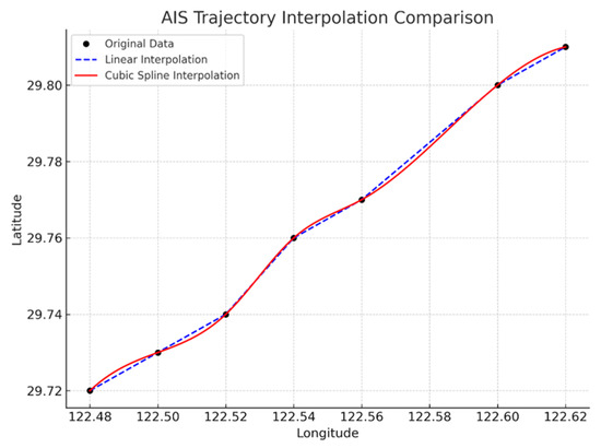
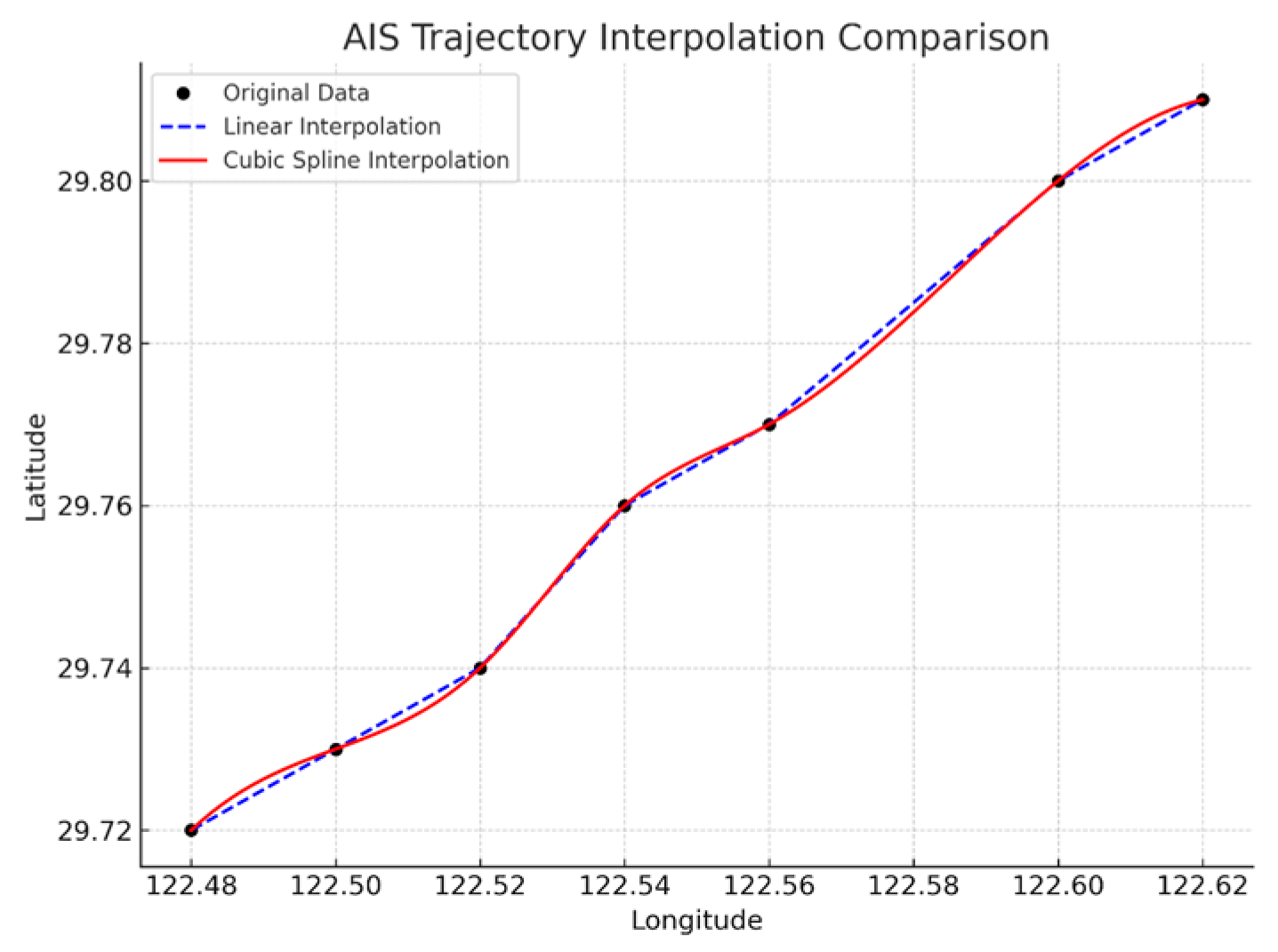
As shown in Figure 1, the black dots represent the original sampled trajectory points, the blue dashed line represents the result of linear interpolation, and the red solid line represents the result of cubic spline interpolation. It can be observed that linear interpolation forms a polyline trajectory by directly connecting adjacent known points. Although linear interpolation is simple and computationally efficient, it may be less capable of representing smooth trajectory transitions in segments with evident turning or speed variation. By contrast, cubic spline interpolation provides a smoother and more continuous approximation of trajectory evolution. Considering smoothness, continuity, and physical plausibility, cubic spline interpolation was ultimately adopted in this study to complete variables such as longitude, latitude, speed, and course, thereby providing a more stable and reliable data foundation for subsequent trajectory prediction modeling.

Figure 1. Interpolation comparison chart.

2.2. Model Development

2.2.1. Overall Model Architecture

To address the pronounced spatiotemporal coupling characteristics of ship trajectory sequences and the difficulty of conventional methods in simultaneously capturing local spatial patterns and long-sequence temporal dependencies, a Spatio-Temporal-Hybrid-Multi-head Attention model, termed STHA, was developed in this study for ship trajectory prediction. The proposed model consists of a convolutional neural network (CNN), a bidirectional long short-term memory network (BiLSTM), and a multi-head attention (MHA) mechanism. First, the CNN module employs convolution kernels of different scales in parallel to extract local spatial variation patterns from trajectory sequences, thereby enhancing the model’s sensitivity to subtle course changes, speed fluctuations, and local trajectory shapes. Subsequently, the BiLSTM is used to model the temporal evolution of the trajectory sequence. By simultaneously exploiting forward and backward temporal information, the model’s ability to represent temporal dependencies at both local and full-window scales is improved. Finally, the multi-head attention mechanism adaptively weights the hidden representations at different time steps, enabling the model to focus more effectively on key historical information that contributes more substantially to the current prediction, thereby improving prediction stability and accuracy in complex maneuvering scenarios.

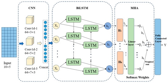
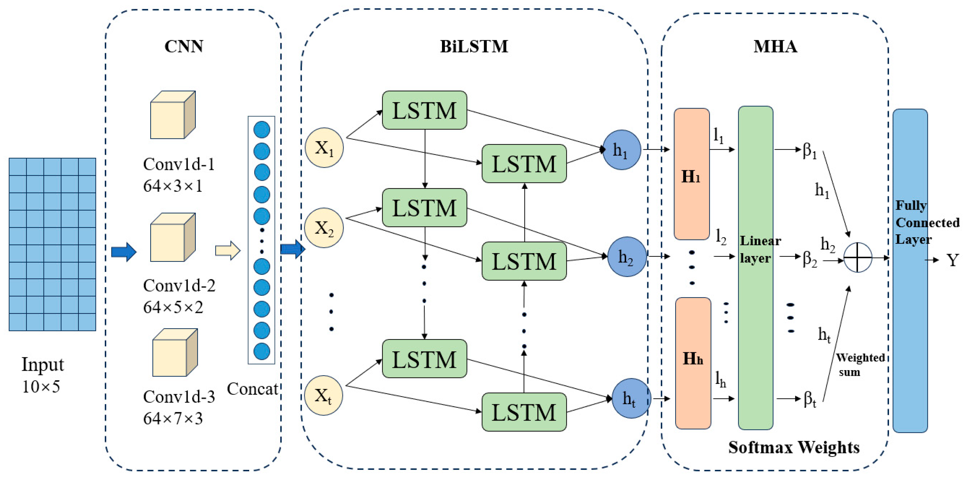
As shown in Figure 2 and Table 1, three parallel one-dimensional convolution branches are arranged at the input stage of the network, with kernel sizes of 3, 5, and 7, respectively, to capture local trajectory features under different receptive fields. The outputs of the three convolution branches are concatenated and then fed into the BiLSTM layer, after which the global temporal representation is further enhanced through the multi-head attention module. Finally, a fully connected layer outputs the predicted longitude, latitude, speed, and course at the next time step. To improve training stability and suppress overfitting, batch normalization and dropout operations are incorporated after both the convolutional and recurrent layers. According to the optimal configuration of the original model, the dimension of the concatenated convolutional features is 192, the output dimension of the BiLSTM is 384, and the output dimension of the attention module is likewise 384, after which continuous-variable regression is completed through linear mapping.

Figure 2. Schematic diagram of the model structure.

Table 1. Model structure parameter settings.

	Network Layer	Output Dimension	Parameters
1	Input	(None, 10, 5)	0
2	Conv1d_1 (kernel = 3)	(None, 10, 64)	1024
3	BatchNorm_1	(None, 10, 64)	128
4	Dropout_1	(None, 10, 64)	0
5	Conv1d_2 (kernel = 5)	(None, 10, 64)	1664
6	BatchNorm_2	(None, 10, 64)	128
7	Dropout_2	(None, 10, 64)	0
8	Conv1d_3 (kernel = 7)	(None, 10, 64)	2304
9	BatchNorm_3	(None, 10, 64)	128
10	Dropout_3	(None, 10, 64)	0
11	Concat (Conv1–3)	(None, 10, 192)	0
12	BiLSTM	(None, 10, 384)	589,824
13	Dropout_4	(None, 10, 384)	0
14	MultiHeadAttention	(None, 10, 384)	589,824
15	Dropout_5	(None, 10, 384)	0
16	Linear (384 → 4)	(None, 4)	1540
17	ReLU	(None, 4)	0

To further improve model performance, Optuna was combined with the CPO strategy in this study to automatically optimize key hyperparameters, including the hidden-layer dimension, the number of BiLSTM layers, the number of attention heads, and the learning rate. As a result, a set of hyperparameters with excellent performance on the validation set and controlled training cost was obtained, thereby providing stable support for performance improvement. The optimal model architecture obtained through Optuna-based hyperparameter tuning is presented in Table 2.

Table 2. Optimal Model Architecture.

Parameter	Value
Hidden dim	192
BiLSTM layer	1
Num heads	2
lr	0.00049356
epochs	32

2.2.2. Multiscale Convolutional Module

For the ship trajectory prediction task, AIS sequences contain coupled local variations in longitude, latitude, speed, and course. Therefore, the convolutional module in this study is used primarily to extract local trajectory variation patterns from sequential AIS data. To enhance the representation of local information at different temporal scales, a multiscale convolutional structure is adopted.

Specifically, the input to the module is a single ship trajectory sequence, rather than multiple trajectories. The same input sequence is processed in parallel by three one-dimensional convolution branches with kernel sizes of 3, 5, and 7, respectively. These parallel branches do not represent three different trajectories; instead, they extract feature representations from the same trajectory sequence under different receptive fields. Smaller kernels help capture fine-grained local disturbances, whereas larger kernels are more suitable for describing local variation trends over relatively wider temporal ranges.

For a local receptive field, the convolution operation can be expressed as

$$Y_i=f_i\left({\displaystyle \sum _{i=1}^n{\omega }_i}{x}_i+b\right)$$

(5)

where $x_i$ denotes the input feature at the $i$-th position within the local receptive field, $w_i$ denotes the corresponding learnable convolution weight, $b$ is the bias term, and $f(\cdot )$ represents the activation function. The convolution output $Y$ is obtained by weighted summation over the local input features followed by nonlinear activation.

In this study, three parallel one-dimensional convolution branches are designed to extract local trajectory features from the same input sequence at different receptive fields. After convolution, the outputs of the three branches are concatenated along the feature dimension to form a richer feature representation. This concatenated feature map is then used as the input to the subsequent BiLSTM module for temporal dependency modeling. In this way, the multiscale convolutional module provides effective local feature support for the following sequence learning process.

2.2.3. Bidirectional Long Short-Term Memory Network Module

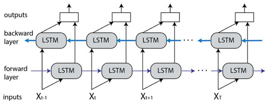
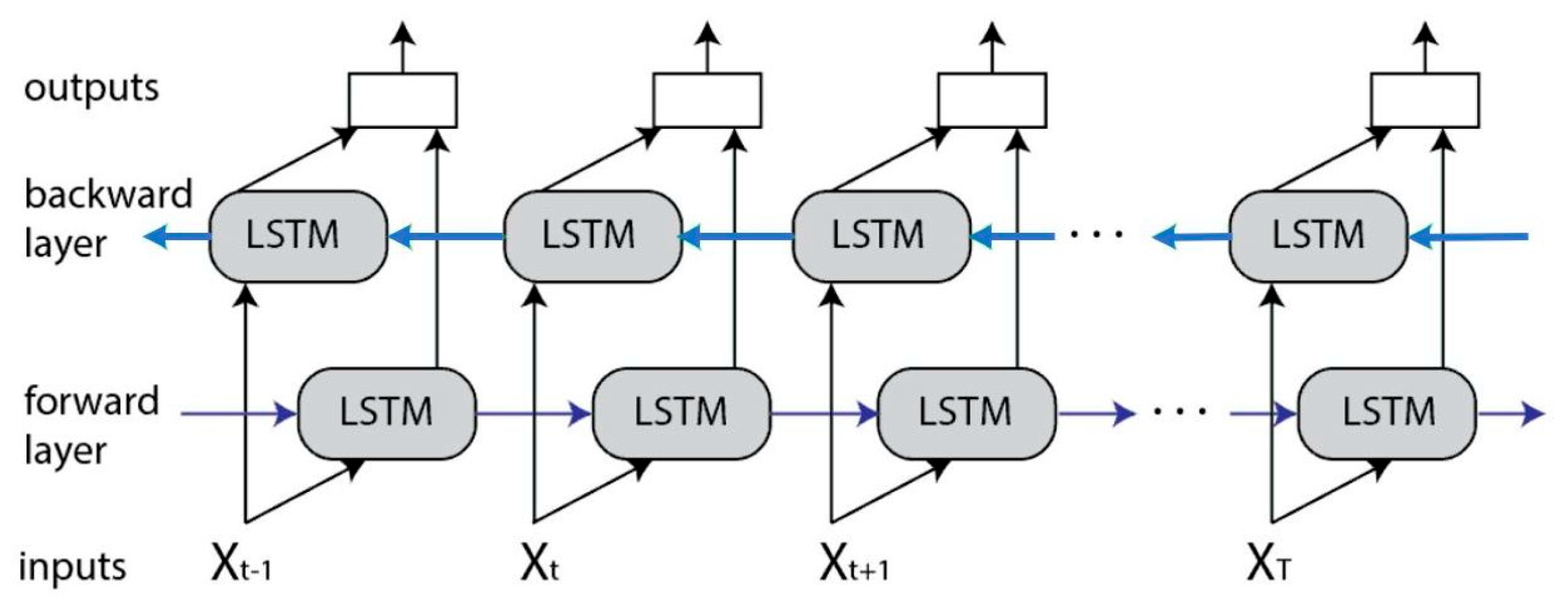
The bidirectional long short-term memory (BiLSTM) network is a bidirectional recurrent neural network architecture designed for sequence data modeling. It exhibits strong feature representation capability when handling long time series and is particularly suitable for capturing long-term dependencies in sequences. Compared with temporal models that propagate information in only a single time direction, BiLSTM introduces both forward and backward information flows, enabling the model to simultaneously exploit historical information and subsequent contextual information at the same time step, thereby obtaining a more complete and coherent sequence representation. The structure of the BiLSTM network is shown in Figure 3.

Figure 3. BILSTM neural network structure diagram.

The BiLSTM architecture consists of a forward LSTM and a backward LSTM, whose basic units still include the cell state, input gate, forget gate, and output gate. The forward network models the input sequence in chronological order, whereas the backward network extracts sequence features in reverse temporal order. Let the input to the BiLSTM at time step $t$ be the convolution-enhanced feature vector $x_t$, which is obtained from the multiscale convolution module. Then, the hidden states of the forward and backward networks can be expressed as

$${\overrightarrow{h}}_t=\overrightarrow{LSTM}\left(x_t,{\overrightarrow{h}}_{t-1}\right)$$

(6)

$${\overleftarrow{h}}_t=\overleftarrow{LSTM}\left(x_t,{\overleftarrow{h}}_{t-1}\right)$$

(7)

The output is obtained by stacking the forward and backward outputs into a combined representation:

$$H_t={\overrightarrow{h}}_t+{\overleftarrow{h}}_t$$

(8)

For ship AIS trajectory prediction, variables such as longitude, latitude, speed, and course exhibit significant continuity and coupling along the temporal dimension, and behaviors such as local turning and speed adjustment usually affect the evolutionary trends of both preceding and subsequent trajectory segments. In this study, AIS trajectories were resampled at 2 min intervals, and each input sequence contained 10 consecutive time steps, corresponding to approximately 20 min of historical motion information. In this context, short-term dependencies refer to local variations over a few adjacent time steps, whereas long-term dependencies refer to dependency relationships across the full input window. Based on this characteristic, a BiLSTM module was introduced after multiscale convolutional feature extraction in this study to further perform temporal modeling on the local features produced by the convolutional module, thereby enhancing the model’s ability to represent both long-term and short-term dependencies in ship trajectories and providing higher-quality temporal representations for the subsequent feature weighting performed by the multi-head attention mechanism.

2.2.4. Multi-Head Attention Module

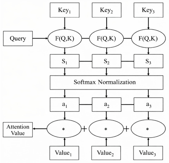
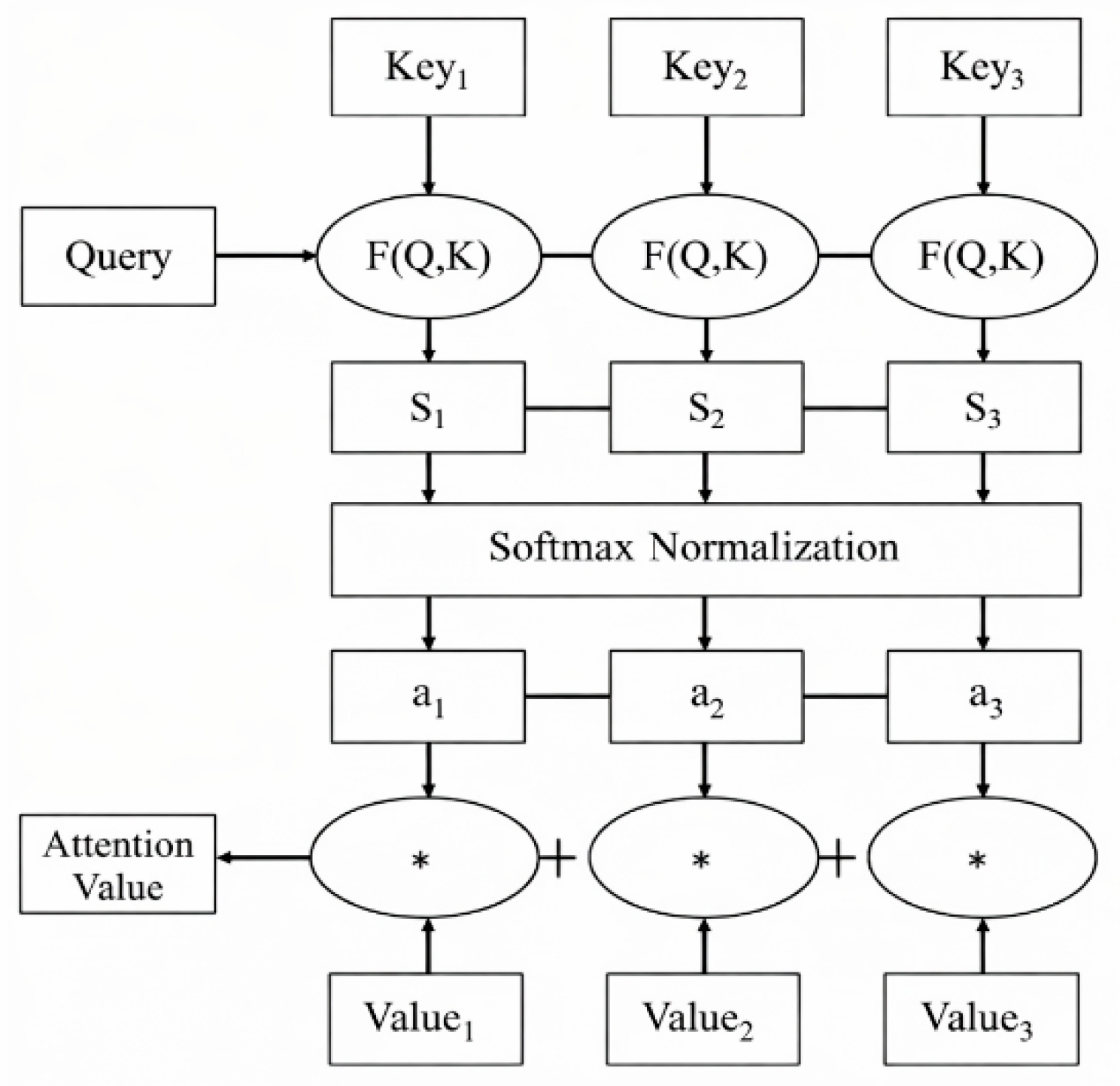
The core idea of the attention mechanism is to assign different weights to input features, enabling the model to focus more on information that is more important for the current task while reducing the influence of less relevant information. In essence, it computes the correlations among input elements, assigns differentiated importance weights to different features, and continuously adjusts these weights during training through gradient descent, thereby improving the model’s ability to extract critical information. In general, the computation of the attention mechanism consists of three stages. First, the similarity between the query vector and the key vector is calculated to measure the relevance of different input elements to the current task. Then, the Softmax function is used to normalize the correlation scores so that they satisfy the properties of a probability distribution. Finally, the normalized weights are used to perform a weighted summation of the value vectors, generating a context vector that reflects the key information. The structure of the attention mechanism network is shown in Figure 4.

Figure 4. Attention mechanism structure.

Here, the input to the attention module is the hidden-state sequence output by the BiLSTM, rather than the raw AIS input variables. In the attention mechanism, the input features are typically passed through three linear mapping layers to obtain the query vector $Q$, key vector $K$, and value vector $V$, respectively. Its basic form can be expressed as,

$$Attention(Q,K,V)=softmax\left({\displaystyle \frac{Q{K}^T}{\sqrt{d_e}}}\right)V$$

(9)

The multi-head attention (MHA) mechanism is a further extension of single-head attention. Its main idea is to map the input features into multiple different subspaces and perform attention calculations in parallel within each subspace. Let the output of the $i$-th attention head be denoted as ${\mathrm{head}}_i$; its computation can be expressed as,

$${\mathrm{head}}_i=\mathrm{Attention}(Q{W}_i^Q,K{W}_i^K,V{W}_i^V)$$

(10)

where $W_i^Q$, $W_i^K$, and $W_i^V$ denote the linear transformation matrices corresponding to the $i$-th attention head. After the outputs of multiple attention heads are concatenated, the final result is obtained through a linear mapping, namely,

$$\mathrm{MultiHead}(Q,K,V)=\mathrm{Concat}({\mathrm{head}}_1,{\mathrm{head}}_2,\dots ,{\mathrm{head}}_h)W^O$$

(11)

where $h$ is the number of attention heads, and $W^O$ is the output projection matrix. Compared with single-head attention, the multi-head attention mechanism can simultaneously learn different types of correlation structures from multiple representation subspaces, thereby enhancing the model’s ability to represent complex feature patterns.

For ship AIS trajectory prediction, variables such as longitude, latitude, speed, and course exhibit complex coupling relationships along the temporal dimension, and the contributions of different historical time steps to the current prediction are not identical. In particular, when a vessel undergoes abrupt turning, speed changes during berthing, or continuous maneuvering, certain key historical moments often contain stronger discriminative information. On this basis, a multi-head attention module was introduced in this study on top of the temporal features extracted by the BiLSTM to adaptively weight the hidden states at different time steps, enabling the model to focus on the historical information that contributes most to the current prediction. Since the multi-head mechanism can learn different representational substructures in parallel across multiple subspaces, it is more conducive to modeling complex vessel behavior patterns and improving both feature representation capability and global dependency modeling in the trajectory prediction process. Finally, the attention-weighted feature representation is fed into a fully connected layer to regress the longitude, latitude, speed, and course at the next time step.

2.3. Experimental Design

In terms of the experimental platform, the hardware environment consisted of a 12th Gen Intel(R) Core(TM) i9-12900K processor and an NVIDIA GeForce RTX 3090 graphics card. The operating system was Windows 11 Professional 64-bit, the programming language was Python 3.9.20, the development environment was PyCharm 2024 Professional Edition, and the deep learning framework was PyTorch 2.7. To improve training efficiency and the rationality of parameter configuration, Optuna was combined with the CPO strategy to automatically search the key model hyperparameters. The resulting optimal parameter combination was as follows: hidden-layer dimension of 192, one BiLSTM layer, two attention heads, a learning rate of 0.00049356, and 32 training epochs. This parameter configuration achieved favorable overall performance on the validation set and was therefore adopted for the subsequent testing experiments.

To objectively evaluate the predictive performance of the STHA model, BP, BiLSTM, and BiGRU were selected as benchmark models. These models were chosen for two reasons. On the one hand, BP refers to a backpropagation-based feedforward neural network. It was included as a basic benchmark model to provide a reference for evaluating the performance improvements brought by deeper temporal architectures and attention-enhanced representations. On the other hand, BiLSTM and BiGRU are both common temporal deep learning models in trajectory prediction research and can reflect the performance of recurrent neural networks in ship trajectory prediction tasks from different perspectives. By comparing STHA with these representative models under the same dataset, the same input window, and the same prediction horizon, the performance improvements brought by the collaborative mechanism of multiscale convolution, bidirectional temporal modeling, and multi-head attention can be more clearly examined.

2.3.1. Dataset Construction

After completing AIS data preprocessing, a sliding-window method was adopted to construct the ship trajectory prediction dataset. Specifically, a historical trajectory sequence of 10 consecutive time steps was used as the model input, and the input features included longitude, latitude, speed, course, and vessel type. During the training stage, the ship state at the 11th time step was taken as the prediction target to construct single-step supervised learning samples. The dataset was divided into a training set, a validation set, and a test set at proportions of 70%, 10%, and 20%, respectively. The training set was used for model parameter learning, the validation set for model selection and hyperparameter optimization, and the test set for final performance evaluation. During the testing stage, a recursive multi-step prediction strategy was adopted, in which the predicted result at the current time step was fed back to the end of the input window and the input sequence was updated in a rolling manner, thereby progressively generating ship trajectory predictions for the next 20 time steps. This setting not only preserves the stability of the training process but also effectively simulates the short- to medium-term trajectory extrapolation process under continuous navigation scenarios.

2.3.2. Evaluation Metrics

To comprehensively assess the performance of ship trajectory prediction models, three typical evaluation metrics were adopted in this study: mean absolute percentage error (MAPE), root mean square error (RMSE), and the coefficient of determination (R²). These three metrics evaluate the model from different perspectives, including the proportional prediction deviation, the magnitude of prediction error, and the goodness of fit, thereby providing a multidimensional and comprehensive analysis of model performance. In this study, the true value refers to the observed AIS value at the target future time step in the dataset, i.e., the ground-truth value used for model evaluation. It does not refer to a continuous trajectory segment between adjacent sampled points.

$$\mathrm{MAPE}={\displaystyle \frac{100\%}{n}}{\displaystyle \sum _{i=1}^n\left|\frac{y_i-{\widehat{y}}_i}{y_i}\right|}$$

(12)

MAPE is used to characterize the average proportional deviation of the predicted values from the true values, and the results are presented in percentage form. A smaller MAPE indicates a smaller discrepancy between the predicted and actual values and, therefore, higher overall prediction accuracy of the model. Owing to its strong interpretability, MAPE is particularly suitable for quantifying the overall level of prediction deviation.

$$\mathrm{RMSE}=\sqrt{{\displaystyle \frac{1}{n}}{\displaystyle \sum _{i=1}^n{\left(y_i-{\widehat{y}}_i\right)}^2}}$$

(13)

RMSE is one of the most commonly used error metrics and reflects the average magnitude of the deviation between the predicted and true values. By taking the square root after averaging the squared errors, RMSE can emphasize the influence of larger deviations on the overall results and therefore has high reference value in prediction tasks that require sensitivity to large errors.

$$R^2=1-{\displaystyle \frac{{\displaystyle \sum _{i=1}^n{(y_i-{\widehat{y}}_i)}^2}}{{\displaystyle \sum _{i=1}^n{(y_i-\overline{y})}^2}}}$$

(14)

The coefficient of determination, R², is used to measure the degree to which the model explains the variance in the data, and its value ranges from 0 to 1. A value closer to 1 indicates that the model fits the actual data better and achieves superior predictive performance. As an important indicator of goodness of fit, R² can directly reflect the correlation between the predicted and actual values.

3. Results

To verify the practical performance of the proposed STHA model in ship trajectory prediction, an overall statistical analysis was first conducted on the trajectory prediction results of 633 vessels in the test set. The results show that the STHA model achieved a mean absolute percentage error (MAPE) of 0.0029%, a root mean square error (RMSE) of 0.0094, and a coefficient of determination (R²) of 0.9902 on the test set. These results indicate that the proposed model exhibits high predictive accuracy and strong fitting capability at the overall sample level. Specifically, the extremely low MAPE suggests that the relative deviation between the predicted and true values is small; the low RMSE indicates that the model can effectively control absolute error and maintain good stability throughout the prediction process; and the R² value of 0.9902 further demonstrates that the model can accurately characterize the variation trends of ship trajectories and has strong explanatory power with respect to the true trajectories. Overall, STHA exhibits favorable comprehensive performance on the large-sample test set, thereby confirming its effectiveness in ship trajectory prediction tasks involving multiple vessel types and diverse scenarios.

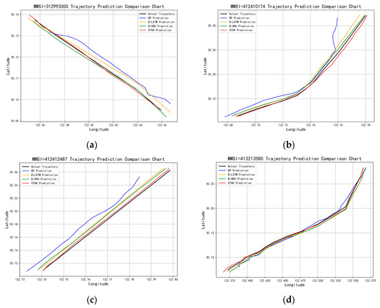
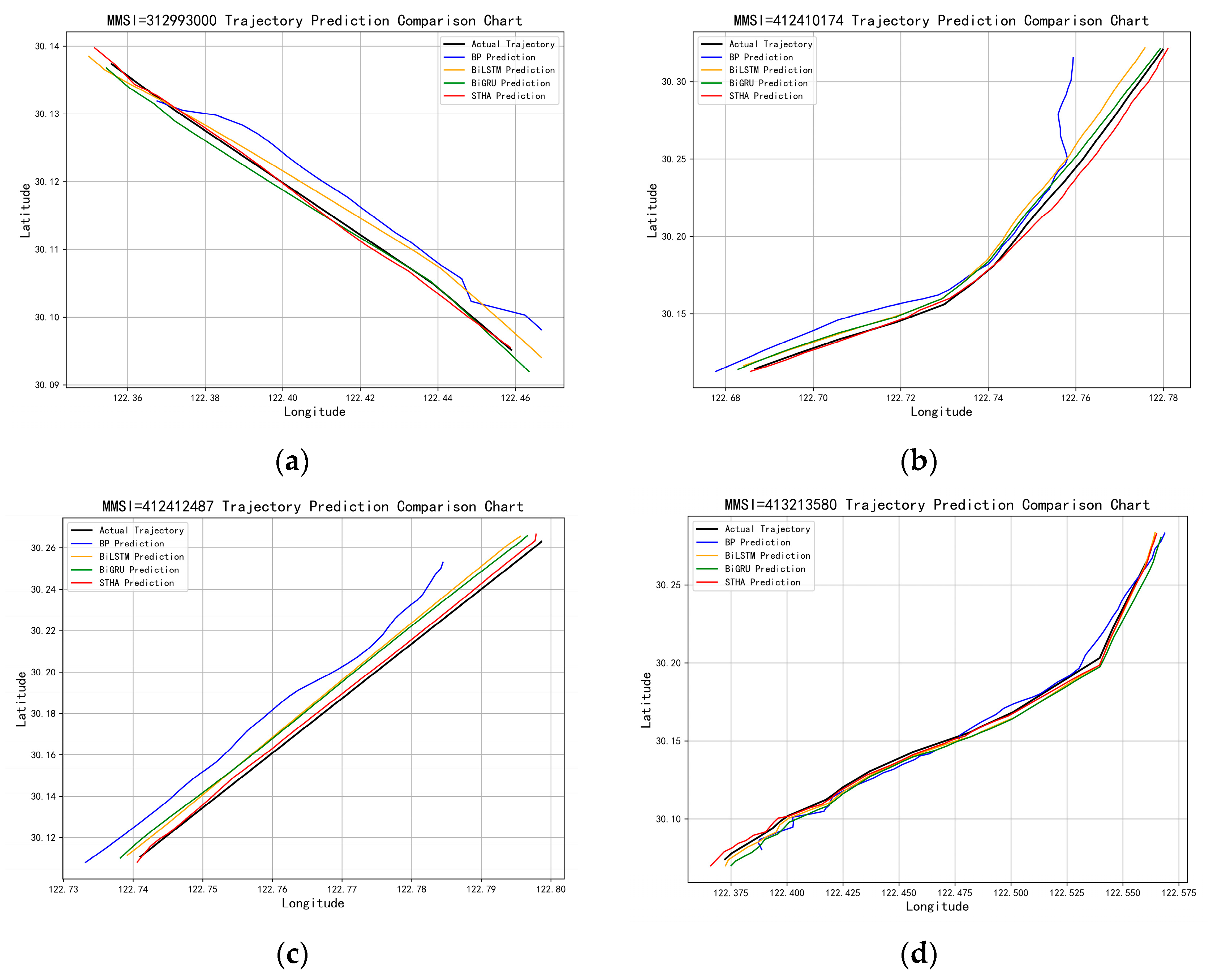
To further analyze the predictive performance of the model in typical scenarios, four representative vessels were selected from the test set for predictive trajectory visualization analysis, namely 312993000 (Cargo), 412410174 (Fishing), 412412487 (Tug), and 413213580 (Tanker). As shown in Figure 5, the trajectory extension trends predicted by different models over future prediction windows of equal length differ markedly. Overall, the trajectories predicted by STHA fit the true trajectories more stably and accurately, with smaller phase lag in both trend extension and turning positions. For the relatively stable trajectories of 312993000 and 412412487, the STHA predictions remain largely consistent with the true trajectories, exhibiting only minor systematic deviations. For the more complex trajectories of 412410174 and 413213580, which involve evident turning, speed variation, or tail-end uplift characteristics, STHA is still able to follow the true variation trends well and demonstrates better smoothness and convergence near turning points. In contrast, the BP model exhibits more pronounced overall deviation and tail-end divergence in multiple samples. Although BiLSTM and BiGRU outperform BP, they still show varying degrees of overestimation, lag, or tail-end drift in some complex maneuvering segments. These results indicate that STHA exhibits strong trajectory fitting capability and predictive stability in both stable navigation segments and complex nonstationary navigation segments.

Figure 5. Comparison of predicted trajectories (a) 312993000; (b) 412410174; (c) 412412487; (d) 413213580.

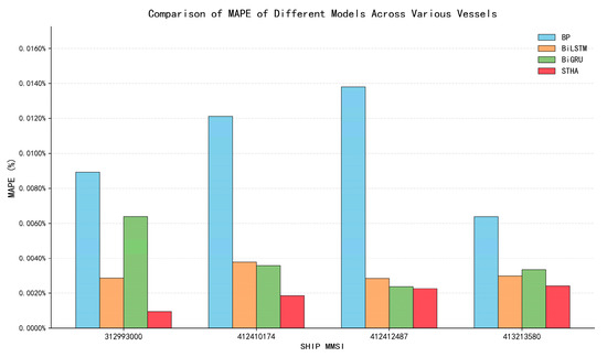
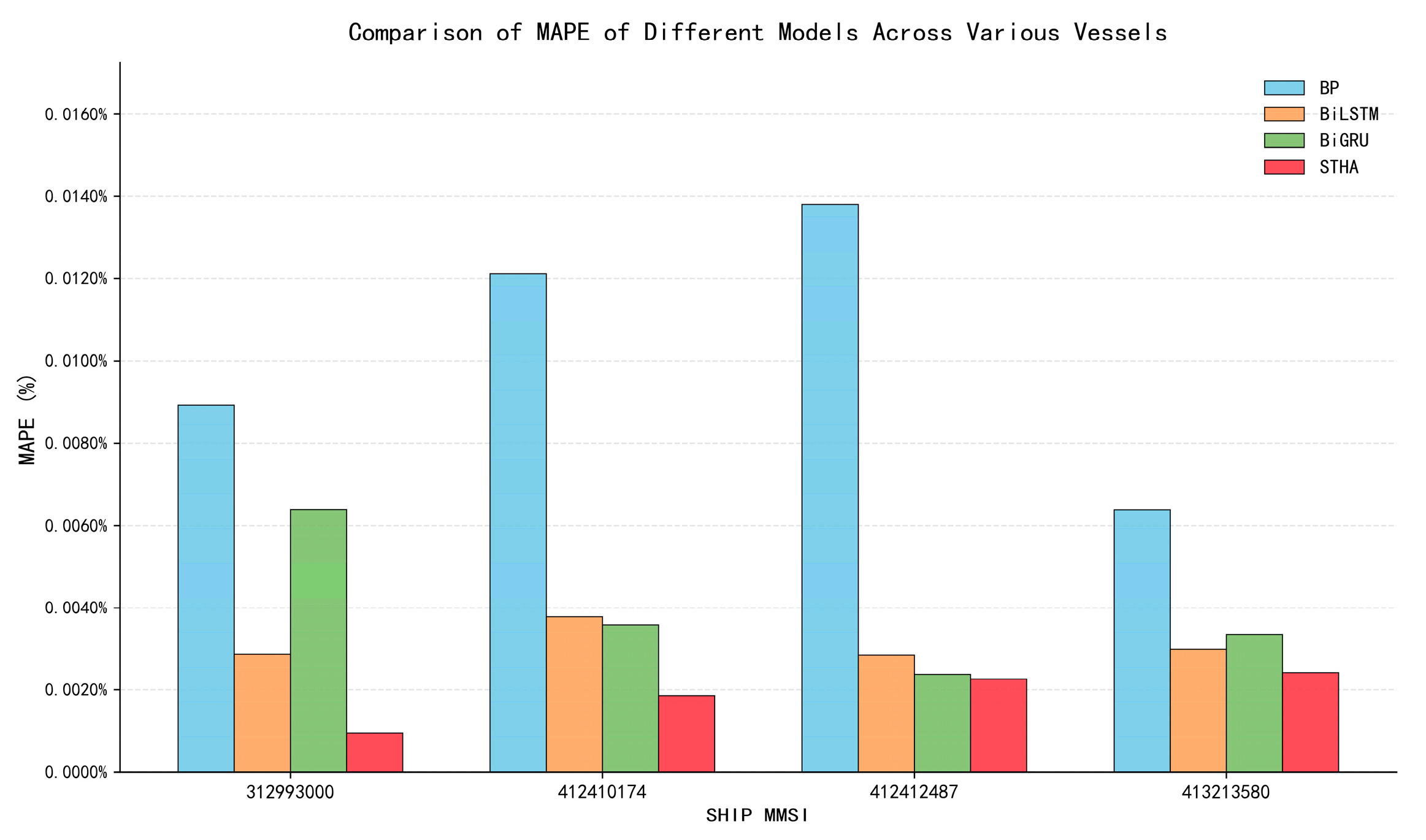
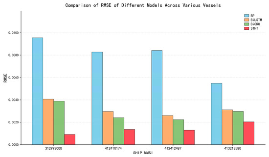
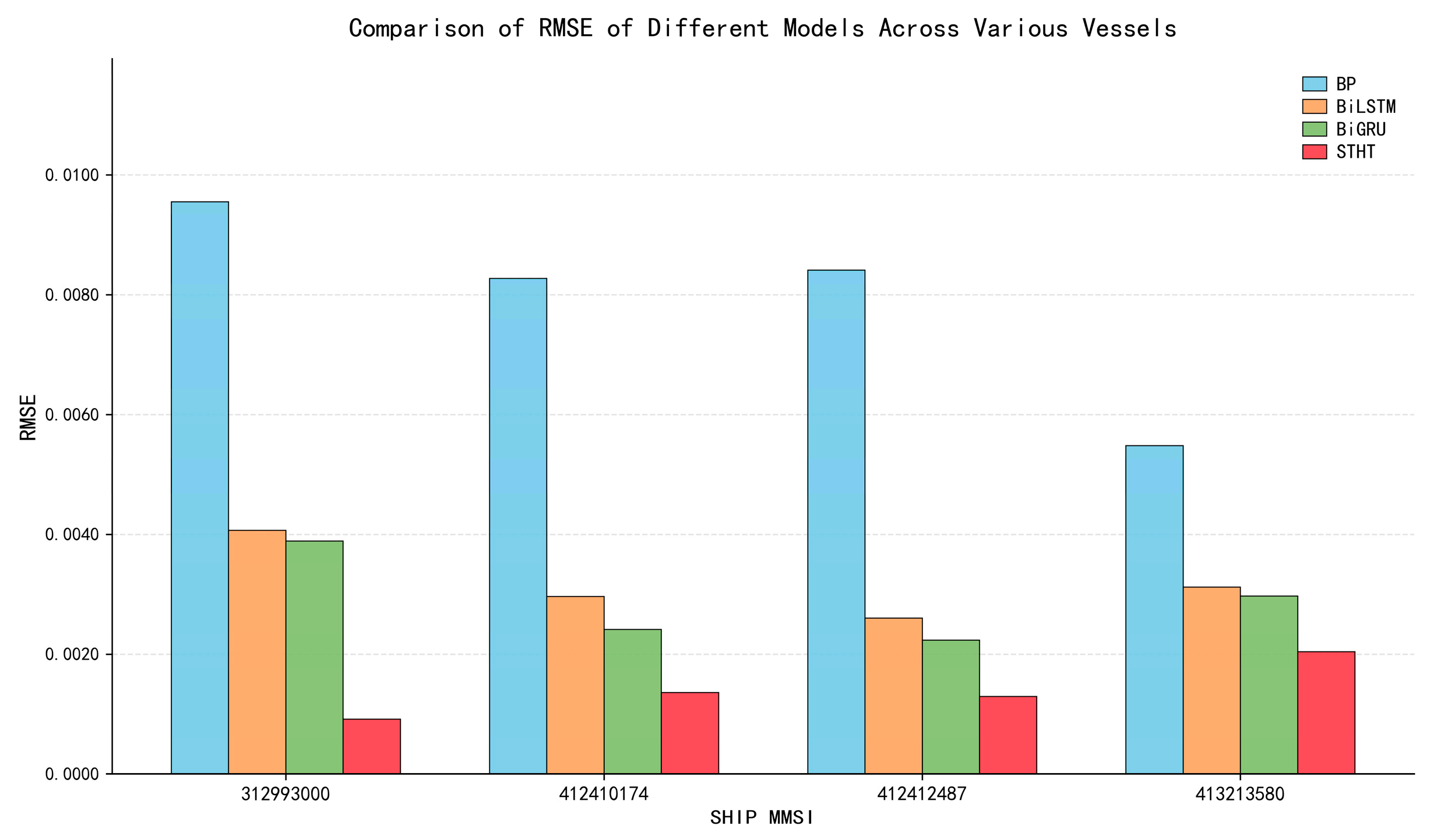
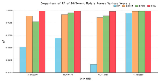
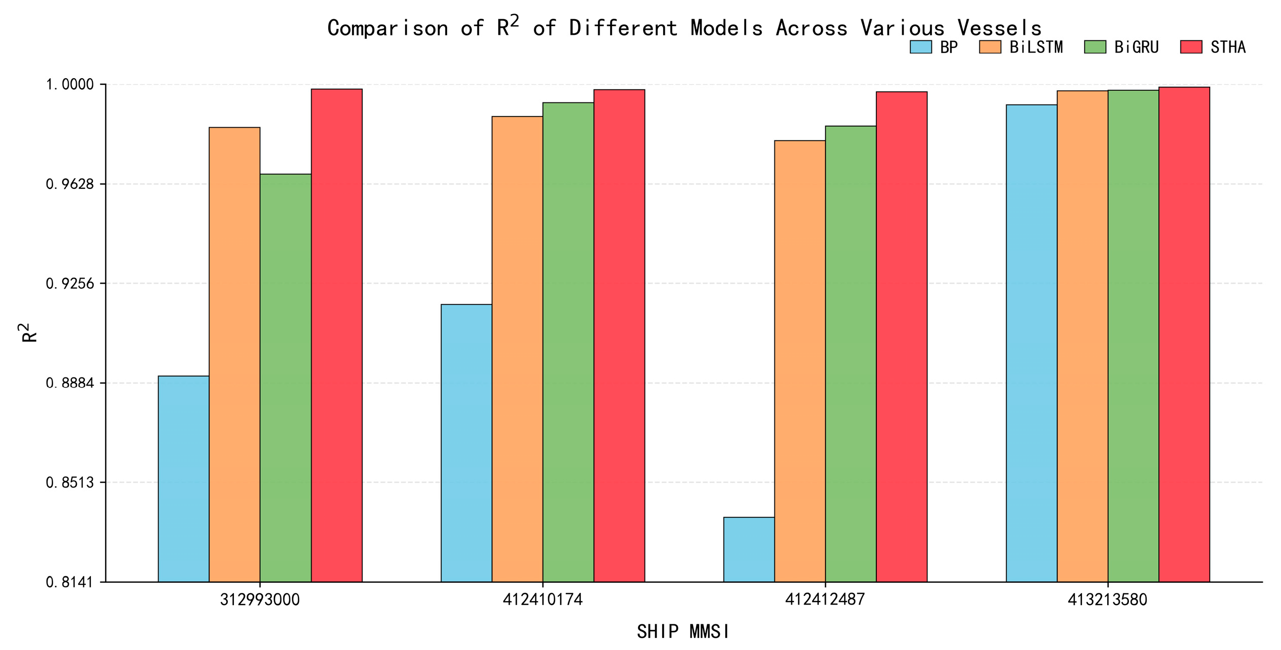
In terms of quantitative metrics, as shown in Figure 6, Figure 7 and Figure 8, a further comparison was conducted for the four representative vessels in terms of MAPE, RMSE, and R². The overall trend was highly consistent: STHA exhibited superior overall performance across all three metrics. In terms of MAPE, STHA achieved the lowest error for all four vessels, with particularly pronounced advantages for MMSI 312993000 and 412410174, indicating a stronger ability to control relative error under scenarios involving complex turning and turning-back maneuvers. In terms of RMSE, the absolute error of STHA consistently remained at a low level and showed the smallest fluctuation range, demonstrating its advantage in suppressing error accumulation and controlling large local deviations. In terms of R², the goodness of fit of STHA for all samples was consistently close to 1, approximately ranging from 0.997 to 0.999, indicating that the model was able to accurately capture the overall variation pattern of the true trajectories. It is noteworthy that, in some cases, although BP also achieved a relatively high R², its MAPE and RMSE remained noticeably larger, suggesting that goodness of fit alone is insufficient to comprehensively reflect prediction quality and that multiple error metrics should be considered jointly for a more complete evaluation. Overall, STHA outperformed BP, BiLSTM, and BiGRU in terms of error level, stability, and fitting capability.

Figure 6. MAPE indicator comparison chart.

Figure 7. RMSE indicator comparison chart.

Figure 8. R² indicator comparison chart.

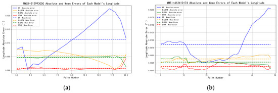
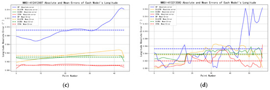
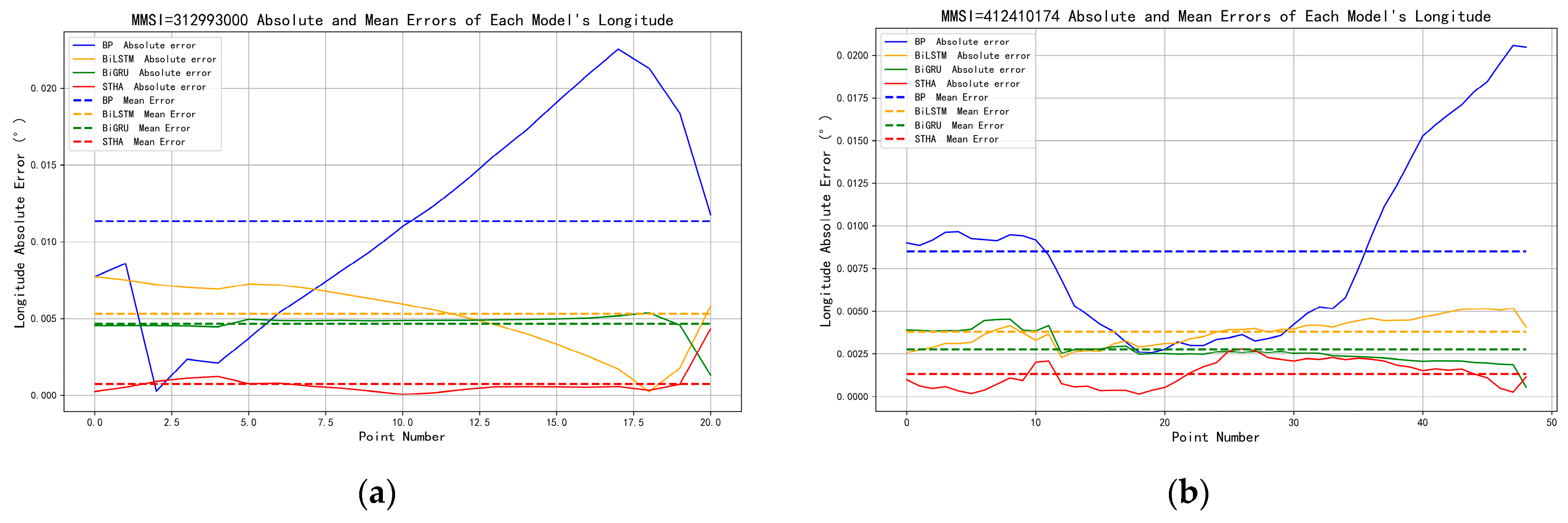
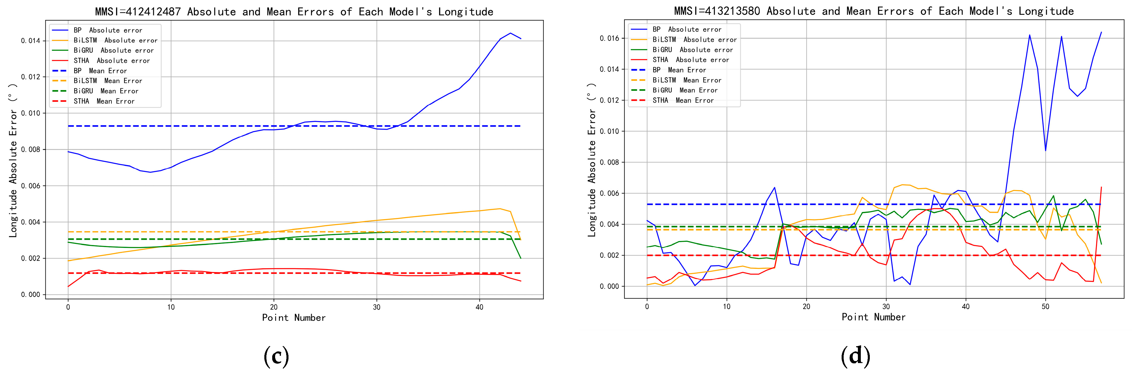
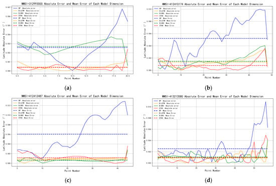
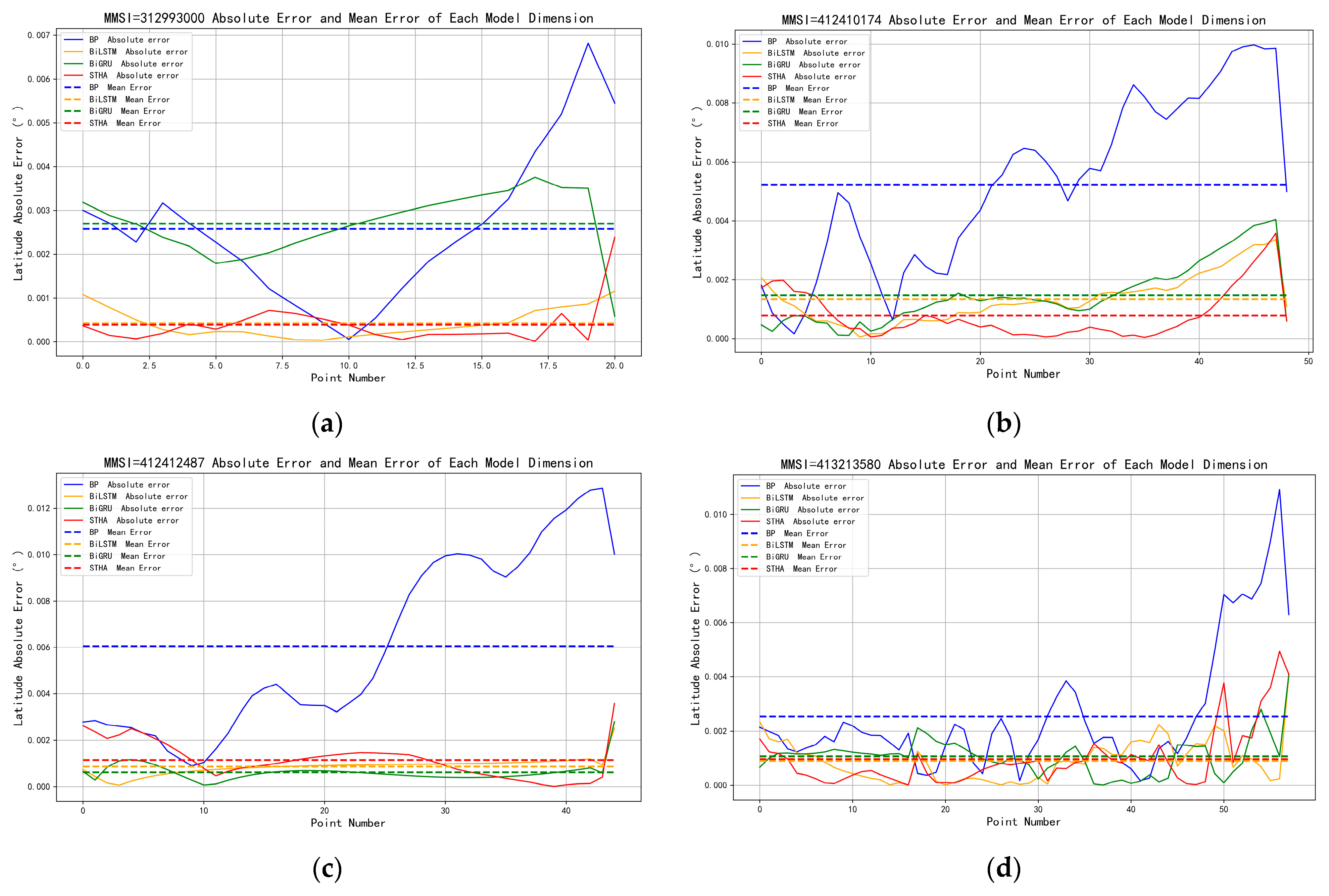
To further analyze the predictive performance of the model with respect to different motion variables, the variations in absolute error were compared separately for longitude, latitude, speed, and course. As shown in Figure 9, in the longitude dimension, the error curve of STHA remains overall closer to the zero axis, and its dashed line representing the average error is almost always the lowest or jointly the lowest. Taking the Cargo and Fishing vessels as examples, the BP model exhibits evident error escalation and tail-end divergence in the middle and later stages, whereas BiLSTM and BiGRU are more stable than BP but still present a certain degree of systematic cumulative deviation. In contrast, STHA maintains relatively low fluctuations in both steady straight-line navigation and repeated turning scenarios, and its error rapidly declines after local disturbances, demonstrating stronger resistance to drift. As shown in Figure 10, in the latitude dimension, STHA likewise exhibits favorable steady-state accuracy and anomaly recovery capability. The Cargo and Fishing samples indicate that BP shows a persistent trend of error accumulation in the middle and later stages, whereas BiLSTM and BiGRU provide some improvement but still remain overall inferior to STHA. For the Tug vessel with a nearly linear navigation segment, the error of STHA remains almost on the zero axis, while for the Tanker vessel, which exhibits multiple small fluctuations in the tail segment, both the peak amplitude and duration of the STHA error are better than those of the benchmark models. These results indicate that STHA not only reduces the average error in spatial coordinates but also effectively mitigates the adverse effect of local error spikes on overall prediction accuracy.

Figure 9. Longitude Error Comparison (a) 312993000; (b) 412410174; (c) 412412487; (d) 413213580.

Figure 10. Latitude Error Comparison (a) 312993000; (b) 412410174; (c) 412412487; (d) 413213580.

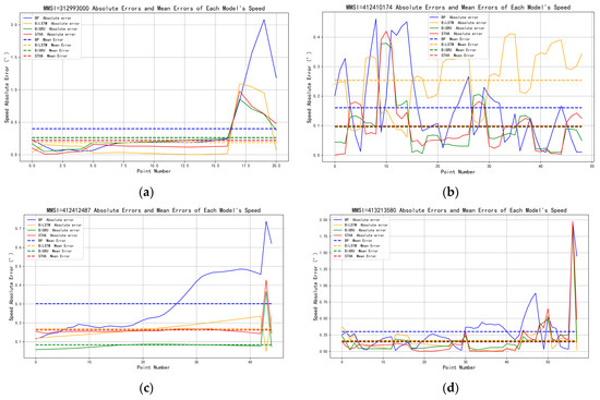
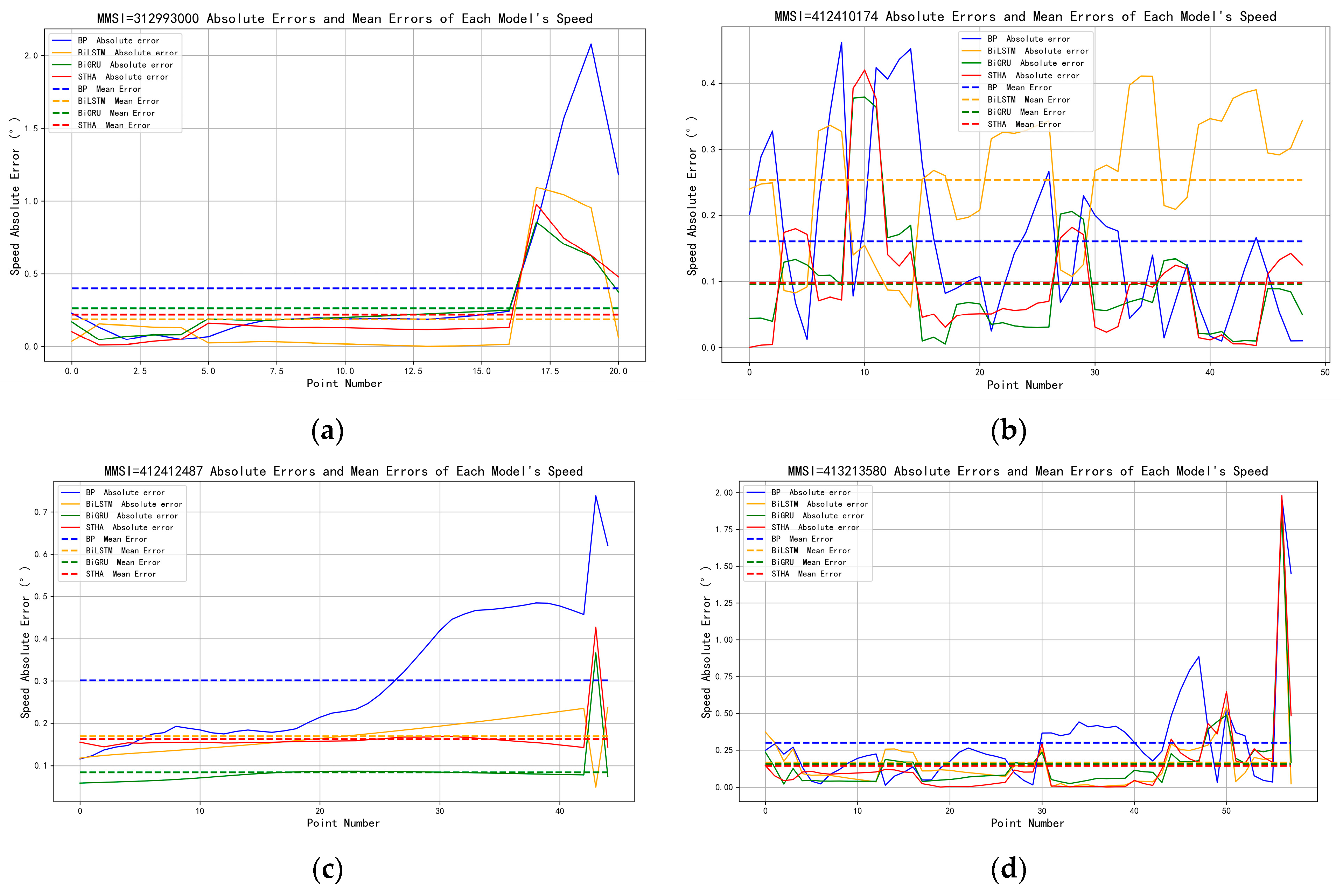
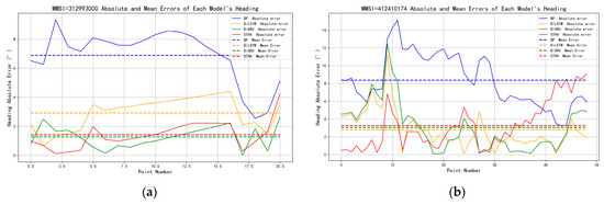
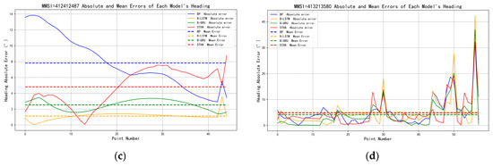
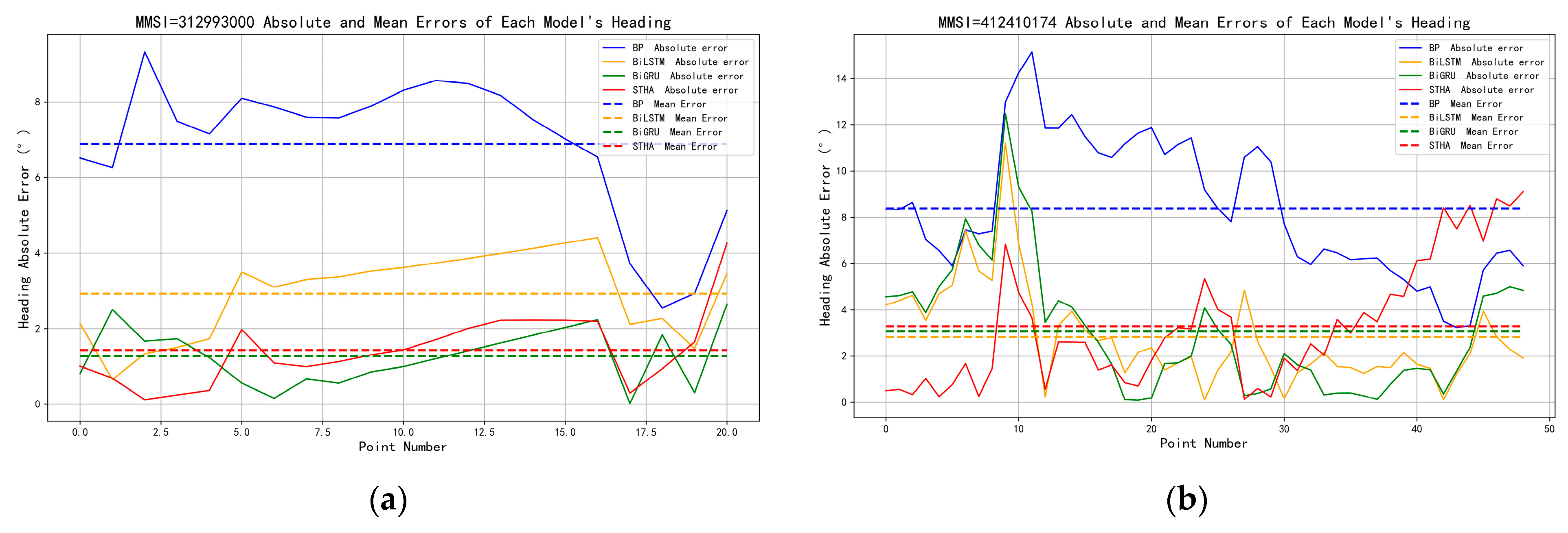
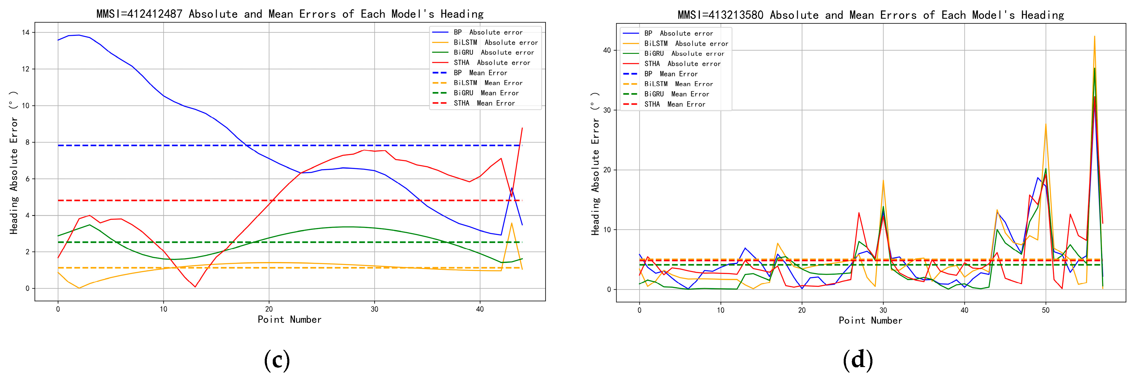
As shown in Figure 11 and Figure 12, STHA also demonstrates strong temporal modeling capability for the two dynamic variables of speed and course. The speed prediction results indicate that the average speed error of STHA is significantly lower than that of BP and BiLSTM and is comparable to or slightly better than that of BiGRU. In the vicinity of typical speed mutation points, such as the local peak regions in the middle and later stages of the Cargo trajectory and in the tail segment of the Tanker trajectory, STHA exhibits smaller error peaks and faster recovery, whereas BP often remains at a high error level or shows secondary oscillations, thereby substantially increasing the overall mean error. For samples such as Fishing, which exhibit evident multi-stage acceleration and deceleration characteristics, STHA is able to track speed variations more smoothly, achieving a balance between dynamic responsiveness and noise resistance. In terms of course prediction, the requirements for phase alignment are higher during turning and course-reversal processes, making this variable more reflective of the model’s ability to characterize complex maneuvering behavior. The results show that STHA maintains relatively low course errors over most navigation segments, and its average error is generally tied for the best performance with BiGRU while being significantly better than that of BP and BiLSTM. In particular, in the dense maneuvering segment of the Fishing trajectory and the abrupt turning segment of the Tanker trajectory, STHA outperforms the benchmark models in terms of peak control, error recovery speed, and overall rhythm matching, indicating that it is better able to achieve synchronized fitting of both the magnitude and phase of course variations.

Figure 11. Speed Error Comparison (a) 312993000; (b) 412410174; (c) 412412487; (d) 413213580.

Figure 12. Heading Error Comparison (a) 312993000; (b) 412410174; (c) 412412487; (d) 413213580.

Overall, the above results indicate that STHA performs consistently across different vessel types, trajectory patterns, and prediction variables. Whether under steady straight-line navigation conditions or in complex scenarios involving evident turning, acceleration and deceleration, and nonlinear tail-end uplift, STHA is able to follow the true trajectory variations more effectively in terms of both magnitude and phase. Its performance advantages mainly stem from the model’s collaborative ability to capture local spatial patterns, long-sequence dependency relationships, and critical historical information. Specifically, the multiscale convolutional module helps extract local trajectory variation features under different receptive fields, BiLSTM enhances the representation of bidirectional temporal dependencies, and the multi-head attention mechanism further improves the model’s ability to identify key historical moments. Therefore, STHA not only outperforms the benchmark models in overall metrics but also exhibits stronger robustness and generalization capability in complex maneuvering scenarios, thereby providing a more reliable input basis for subsequent collision risk assessment and warning based on predicted trajectories.

4. Discussion

The results demonstrate that the proposed STHA model achieves favorable performance in AIS-based ship trajectory prediction and shows clear advantages over BP, BiLSTM, and BiGRU in terms of MAPE, RMSE, and R² under the present experimental setting. In particular, STHA is better able to follow true trajectory variations across different vessel types and trajectory patterns and exhibits stronger robustness in dynamic maneuvering scenarios involving turning, course changes, and acceleration or deceleration.

Further analysis suggests that these improvements mainly stem from the collaborative effects of the three core components of the model. The multiscale convolutional module helps extract local spatial variation patterns from trajectory sequences under different receptive fields, BiLSTM enhances the representation of local temporal variations and longer-range dependencies, and the multi-head attention mechanism improves the model’s ability to identify and utilize critical historical information. As a result, the proposed framework shows improved resistance to error accumulation and tail-end drift in non-stationary navigation segments.

Compared with previously reported ship trajectory prediction studies, the proposed STHA model demonstrates competitive predictive performance. However, direct numerical comparisons across studies should be interpreted with caution, because datasets, study areas, preprocessing procedures, input settings, prediction horizons, and evaluation criteria are often different. Therefore, the present results mainly demonstrate the effectiveness and robustness of the proposed model within the current experimental framework.

Although this study was conducted using AIS data from the Zhoushan waters, the proposed STHA framework is not inherently restricted to this specific region. With appropriate data preprocessing, feature standardization, and parameter adaptation, the model may also be extended to other vessel trajectory prediction scenarios, such as different coastal waters, port traffic environments, and other short- to medium-term maritime trajectory forecasting tasks. Nevertheless, its performance under different traffic densities, navigation structures, and environmental conditions still requires further validation.

Overall, the proposed model provides a useful approach for high-precision ship trajectory prediction and may offer valuable support for downstream applications such as collision risk assessment and navigation safety assistance. Future work may further investigate the transferability of the model across different regions and incorporate additional influencing factors, such as multi-vessel interactions, meteorological and oceanographic conditions, and waterway environments, to improve its applicability and generalization capability in more complex maritime scenarios.

References

- Perera, L.P. Navigation vector based ship maneuvering prediction. Ocean Eng. 2017, 138, 151–160. [Google Scholar] [CrossRef] [Scilit]
- Liu, X.; Xiong, F. Long-distance prediction system for ship grounding based on sensor networks. Ship Sci. Technol. 2021, 43, 43–46. [Google Scholar]
- Tong, X.; Chen, X.; Sang, L.; Mao, Z.; Wu, Q. Vessel trajectory prediction in curving channel of inland river. In Proceedings of the 2015 International Conference on Transportation Information and Safety (ICTIS), Wuhan, China, 25–28 June 2015; IEEE: Piscataway, NJ, USA, 2015; pp. 706–714. [Google Scholar]
- Luo, W.; Zhang, G. Ship Motion Trajectory and Prediction Based on Vector Analysis. J. Coast. Res. 2020, 95, 1183–1188. [Google Scholar] [CrossRef] [Scilit]
- Li, R. Mathematical model design for ship navigation trajectory prediction. Ship Sci. Technol. 2020, 42, 13–15. [Google Scholar]
- Martelli, M.; Žułkin, S.; Zaccone, R.; Rudan, I. A COLREGs -compliant decision support tool to prevent collisions at sea. Int. J. Mar. Navig. Saf. Sea Transp. 2023, 17, 347–353. [Google Scholar] [CrossRef] [Scilit]
- Hu, L.; Hu, H.; Naeem, W.; Wang, Z. A review on COLREGs-compliant navigation of autonomous surface vehicles: From traditional to learning-based approaches. J. Autom. Intell. 2022, 1, 100003. [Google Scholar] [CrossRef] [Scilit]
- Zhang, Z.; Zhao, J.; Wang, T.; Ma, F.; Diaconeasa, M.A. Motion prediction of tugboats using hidden Markov model. In Proceedings of the 2023 7th International Conference on Transportation Information and Safety, Xi’an, China, 4–6 August 2023; pp. 621–627. [Google Scholar] [CrossRef] [Scilit]
- Sang, L.; Yan, X.; Wall, A.; Wang, J.; Mao, Z. CPA calculation method based on ais position prediction. J. Navig. 2016, 69, 1409–1426. [Google Scholar] [CrossRef] [Scilit]
- Zhang, Z.; Fu, K.; Sun, X.; Ren, W. Multiple target tracking based on multiple hypotheses tracking and modified ensemble Kalman filter in multi-sensor fusion. Sensors 2019, 19, 3118. [Google Scholar] [CrossRef] [Scilit]
- Maskooki, A.; Virjonen, P.; Kallio, M. Assessing the prediction uncertainty in a route optimization model for autonomous maritime logistics. Int. Trans. Oper. Res. 2021, 28, 1765–1786. [Google Scholar] [CrossRef] [Scilit]
- Chen, G.; Wang, W.; Xue, Y. Identification of ship dynamics model based on sparse gaussian process regression with similarity. Symmetry 2021, 13, 1956. [Google Scholar] [CrossRef] [Scilit]
- Rong, H.; Teixeira, A.P.; Soares, C.G. Maritime traffic probabilistic prediction based on ship motion pattern extraction. Reliab. Eng. Syst. Saf. 2022, 217, 108061. [Google Scholar] [CrossRef] [Scilit]
- Borkowski, P. The ship movement trajectory prediction algorithm using navigational data fusion. Sensors 2017, 17, 1432. [Google Scholar] [CrossRef] [Scilit] [PubMed]
- Gan, S.; Liang, S.; Li, K.; Deng, J.; Cheng, T. Ship trajectory prediction for intelligent traffic management using clustering and ANN. In Proceedings of the 2016 UKACC 11th International Conference on Control, Belfast, UK, 31 August–2 September 2016; pp. 1–6. [Google Scholar]
- Yang, C.H.; Lin, G.C.; Wu, C.H.; Liu, Y.H.; Wang, Y.C.; Chen, K.C. Deep learning for vessel trajectory prediction using clustered AIS data. Mathematics 2022, 10, 2936. [Google Scholar] [CrossRef] [Scilit]
- Murray, B.; Perera, L.P. Ship behavior prediction via trajectory extraction-based clustering for maritime situation awareness. J. Ocean Eng. Sci. 2022, 7, 1–13. [Google Scholar] [CrossRef] [Scilit]
- Zheng, Y.; Zhang, X.; Shang, Z.; Guo, S.; Du, Y. A decision-making method for ship collision avoidance based on improved cultural particle swarm. J. Adv. Transp. 2021, 2021, 8898507. [Google Scholar] [CrossRef] [Scilit]
- Karataş, G.B.; Karagoz, P.; Ayran, O. Trajectory pattern extraction and anomaly detection for maritime vessels. Internet Things 2021, 16, 100436. [Google Scholar] [CrossRef] [Scilit]
- Zhang, C.; Bin, J.; Wang, W.; Peng, X.; Wang, R.; Halldearn, R.; Liu, Z. AIS data driven general vessel destination prediction: A random forest based approach. Transp. Res. Part C Emerg. Technol. 2020, 118, 102729. [Google Scholar] [CrossRef] [Scilit]
- Abebe, M.; Shin, Y.; Noh, Y.; Lee, S.; Lee, I. Machine learning approaches for ship speed prediction towards energy efficient shipping. Appl. Sci. 2020, 10, 2325. [Google Scholar] [CrossRef] [Scilit]
- Chen, K.; Zhu, Y.; Yan, K.; Cai, K.; Ren, Z.; Gao, D. Ship trajectory prediction based on LSTM. Ship Ocean Eng. 2019, 48, 121–125. [Google Scholar]
- Liu, T.; Ma, J. Ship navigation behavior prediction based on AIS data. IEEE Access 2022, 10, 47997–48008. [Google Scholar] [CrossRef] [Scilit]
- Murray, B.; Perera, L.P. A dual linear autoencoder approach for vessel trajectory prediction using historical ais data. Ocean Eng. 2020, 209, 107478. [Google Scholar] [CrossRef] [Scilit]
- Li, Y.; Ren, H. Vessel traffic flow prediction using LSTM encoder-decoder. In Proceedings of the International Conference on Signal Processing and Machine Learning, Dalian, China, 4–6 August 2022; pp. 1–7. [Google Scholar]
- Yang, C.; Wu, C.; Shao, J.; Wang, Y.; Hsieh, C. AIS-based intelligent vessel trajectory prediction using Bi-LSTM. IEEE Access 2022, 10, 24302–24315. [Google Scholar] [CrossRef] [Scilit]
- Park, J.; Jeong, J.; Park, Y. Ship trajectory prediction based on Bi-LSTM using spectral-clustered ais data. J. Mar. Sci. Eng. 2021, 9, 1037. [Google Scholar] [CrossRef] [Scilit]
- Jiang, J.; Zuo, Y. Prediction of ship trajectory in nearby port waters based on attention mechanism model. Sustainability 2023, 15, 7435. [Google Scholar] [CrossRef] [Scilit]
- Zhong, C.; Jiang, Z.; Chu, X.; Liu, L. Inland ship trajectory restoration by recurrent neural network. J. Navig. 2019, 72, 1359–1377. [Google Scholar] [CrossRef] [Scilit]
- Suo, Y.; Chen, W.; Claramunt, C.; Yang, S. A ship trajectory prediction framework based on a recurrent neural network. Sensors 2020, 20, 5133. [Google Scholar] [CrossRef] [Scilit]
- Zhang, L.; Zhang, J.; Niu, J.; Wu, Q.M.J.; Li, G. Track prediction for HF radar vessels submerged in strong clutter based on MSCNN fusion with GRU-AM and AR model. Remote Sens. 2021, 13, 2164. [Google Scholar] [CrossRef] [Scilit]
- Wang, C.; Ren, H.; Li, H. Vessel trajectory prediction based on AIS data and bidirectional GRU. In Proceedings of the International Conference on Computer Vision, Image and Deep Learning, Chongqing, China, 10–12 July 2020; pp. 260–264. [Google Scholar]
- Chen, J.; Chen, H.; Zhao, Y.; Li, X. FB-BiGRU: A deep learning model for AIS-based vessel trajectory curve fitting and analysis. Ocean Eng. 2022, 266, 112898. [Google Scholar] [CrossRef] [Scilit]
Disclaimer/Publisher’s Note: The statements, opinions and data contained in all publications are solely those of the individual author(s) and contributor(s) and not of MDPI and/or the editor(s). MDPI and/or the editor(s) disclaim responsibility for any injury to people or property resulting from any ideas, methods, instructions or products referred to in the content. |
© 2026 by the authors. Licensee MDPI, Basel, Switzerland. This article is an open access article distributed under the terms and conditions of the Creative Commons Attribution (CC BY) license.