


Abstract
The complexity of modern vehicle control systems, the increasing diversity of powertrain and exhaust aftertreatment applications, and the need for shortened development times require innovative approaches towards calibration. This paper presents an experimental, analytical, and modeling study of particulate filter (commonly called DPF—diesel particulate filter) in a diesel hybrid vehicle where models have been developed to simulate test data, replacing the requirement of numerous tests on testbed or on the road with system simulations and offline parameter optimisation techniques. A soot estimation model has been developed based on the operation of the engine including its transient response, and the thermal–chemical behaviour of the DPF. A methodology has been developed to optimize the calibratable maps and parameters within this model. The results show that the proposed method improves the accuracy of soot estimation in the engine transient operation and avoids a large number of experimental tests required in traditional calibration methods. Modern automotive manufacturers face regulatory compliance requirements ensuring emission standards across diverse real driving emission (RDE) boundary conditions encompassing route characteristics, driving dynamics, and ambient environmental variables throughout vehicles’ operational lifetime. The soot load in the DPF and the DPF regeneration frequency can massively impact the tailpipe NOx emissions and overall fuel consumption, so it is key to accurately estimate the soot accumulation in all operating conditions. This means testing and validating calibration in each possible scenario and so needs an enormous number of tests on testbed and on the road. These tests, however, can be replaced with system simulations and offline calibration if we have a robust model for the system, as described in the following parts of this paper.
1. Introduction
The development of comprehensive frameworks for optimising exhaust aftertreatment control strategies through advanced computational modeling techniques represents a critical pathway toward reducing real-world tailpipe emissions, particularly those quantified under RDE test protocols. The implementation of RDE compliance testing introduces unprecedented challenges and complexity to contemporary vehicle development approaches. European emission legislation continues evolving toward increasingly stringent requirements, with Euro 7 standards combined with RDE protocols presenting formidable challenges for internal combustion engine-based vehicle platforms in the coming regulatory period.
Exhaust emission control technologies have experienced substantial advancement over the past two decades, with significant potential still present for further emission reductions through the optimisation of existing systems combined with innovative aftertreatment concepts [1]. While no single technological solution provides complete emission mitigation, appropriate technology combinations and innovations can achieve unprecedented cleanliness levels in ICE-based powertrains. Diverse technologies spanning combustion optimisation, catalytic conversion, and particulate capture are under active research and development to reduce pollutant emissions meeting stringent Euro 7 targets and subsequent regulations, targeting near-zero emission levels.
Particulate matter represents one of the primary pollutants emitted by internal combustion engines with documented adverse human health impacts [2]. Diesel particulate filtration technology provides the most effective approach for reducing particulate emissions in diesel engines [3,4] where modern systems capture over 90% of engine-out particulates [5,6,7]. However, gradual soot accumulation within DPF systems increases the exhaust back pressure, leading to engine efficiency degradation and increased fuel consumption [8]. Consequently, the continuous or periodic removal of accumulated soot from DPF systems becomes necessary [9,10].
Optimal DPF regeneration timing requires precise soot load estimation accuracy. Various methodologies have been developed for soot load estimation; however, challenging operational conditions including low volumetric flow rates and transient engine operation cause estimation inaccuracies [11,12]. The most prevalent soot load monitoring approach derives from pressure drop relationships across DPF systems relative to soot accumulation. Nevertheless, engine exhaust represents extremely volatile airflow characteristics, intensified under transient operating conditions. Consequently, pressure sensor measurements exhibit significant noise, causing substantial deviations in soot load calculations based on these signals.
Recent regulatory developments emphasize vehicle emission compliance across all possible real-world road conditions, extending DPF operational scrutiny including soot load and regeneration events to all RDE test cycles. This introduces additional complexity to accurate soot estimation optimisation, requiring numerous tests covering all operating conditions. Transferring the majority of the calibration effort from physical test cells and road testing to the desktop through modeling and simulation represents a solution to these pressing challenges.
This research presents this approach and validates a soot estimation model optimized for real-world driving cycles. The model was developed to calculate soot accumulation based on engine operation and DPF thermal–chemical behaviour characteristics. The model incorporates soot oxidation rates by nitrogen dioxide (NO2) through the determination of NO to NO2 conversion rates and NO2 utilisation rates for carbon oxidation [13,14]. A comprehensive methodology supported by advanced automated optimisation routines was developed for calibrating adjustable maps and parameters. Validation was performed using vehicle test data collected on chassis dynamometer and on-road testing utilising an AVL Micro-Soot-Sensor (MSS), demonstrating adequate soot estimation accuracy across various driving cycles.
2. IC Engine Emissions and Legislation
The internal combustion engines generate mechanical work from chemically bound fuel energy through combustion processes. Beyond complete combustion products (carbon dioxide CO2 and water H2O), combustion processes generate undesirable pollutants, primarily carbon monoxide (CO), unburnt hydrocarbons (HCs), nitrogen oxides (NOx), and particulate matter (PM) [4,15].
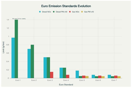
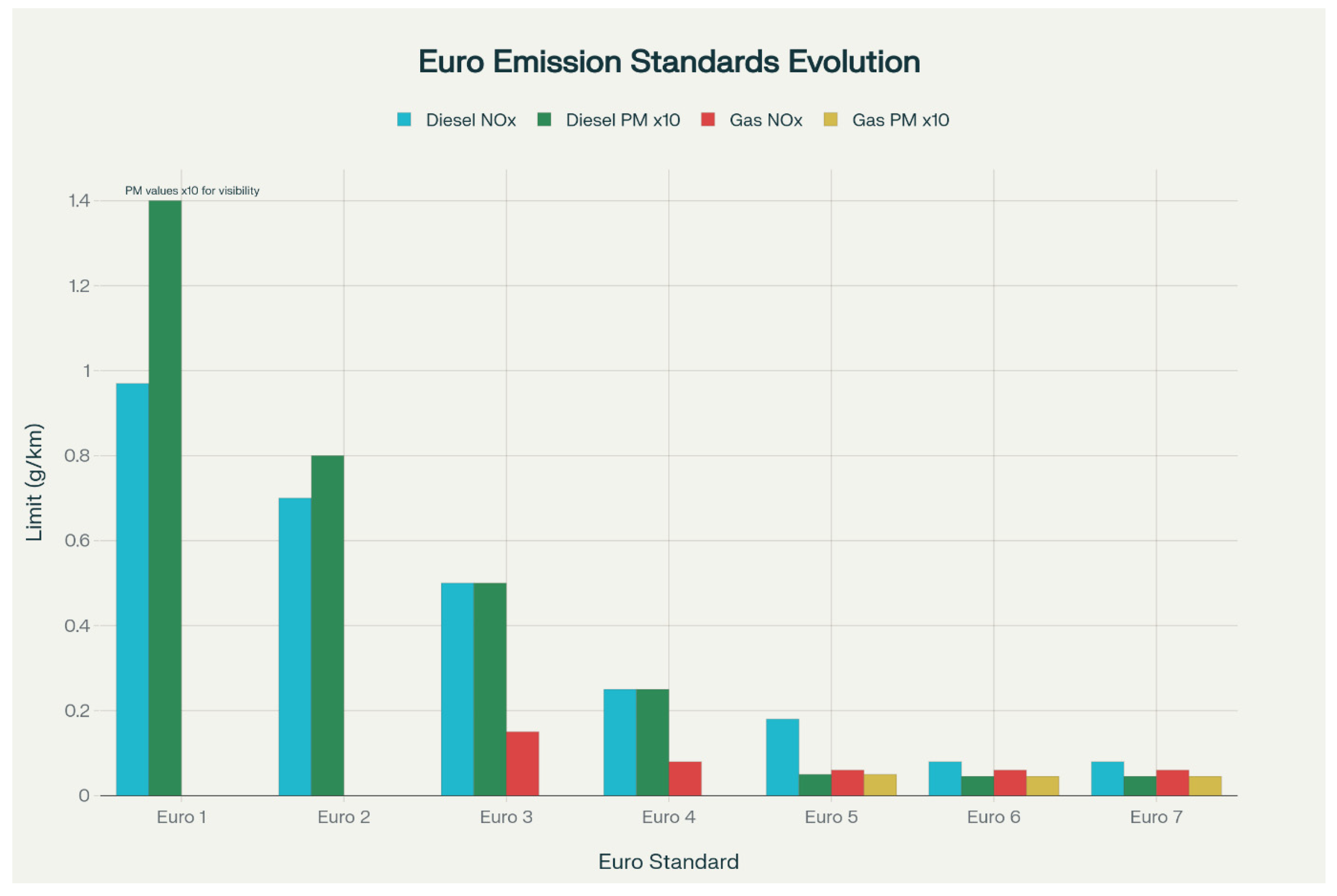
Engine pollutants have been regulated for passenger cars and commercial vehicles since emission legislation was introduced with Euro 1 standards in Europe. European emission standards for passenger cars demonstrate gradual significant reductions across all emissions from Euro 1 to the upcoming Euro 7 as shown in Figure 1.
Figure 1.
European emission limit values for passenger cars.
The evolution of these standards has been remarkable, with each successive regulation imposing more stringent limits on pollutant emissions. Beginning with Euro 5’s implementation for passenger cars, minimal particulate levels have been universally achieved through DPF utilisation [4,16]. Euro 6 standards introduced particle concentration limits for commercial vehicles, making universal DPF implementation inevitable for commercial vehicle engines [17,18].
Current Euro 6 emission standards specifically noted that considerable reduction in NOx emissions from diesel vehicles was necessary to improve air quality and comply with limit values for air pollution [19]. It is expected that Euro 7 standards will further improve air quality.
3. Emissions Control Strategies
Contemporary emission control strategies for gasoline vehicles maintain Euro 6 standards largely unchanged from Euro 5, except for new particle number standards for gasoline direct injection (GDI) vehicles, previously applied only to diesel vehicles in Euro 5. As CO2 targets continue decreasing, GDI engine technology has matured and is increasingly deployed. GDI engines produce higher particle emissions than conventional port fuel injection gasoline engines, hence the particle number limit introduction to prevent gasoline vehicle particle emission increases.
For diesel vehicles, reduced NOx limits require manufacturers to utilize advanced aftertreatment technologies alongside exhaust gas recirculation (EGR) systems [20,21]. Aftertreatment technologies including lean NOx traps (LNTs) and selective catalytic reduction (SCR) are integrated with technologies already adopted for CO, HC, and PM control, including diesel oxidation catalysts (DOCs) and diesel particulate filters (DPFs). Since higher NOx emissions can result from engine calibrations designed to maximise fuel economy, advanced NOx aftertreatment could allow such calibrations without NOx emission increases.
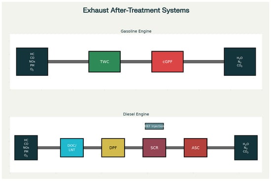
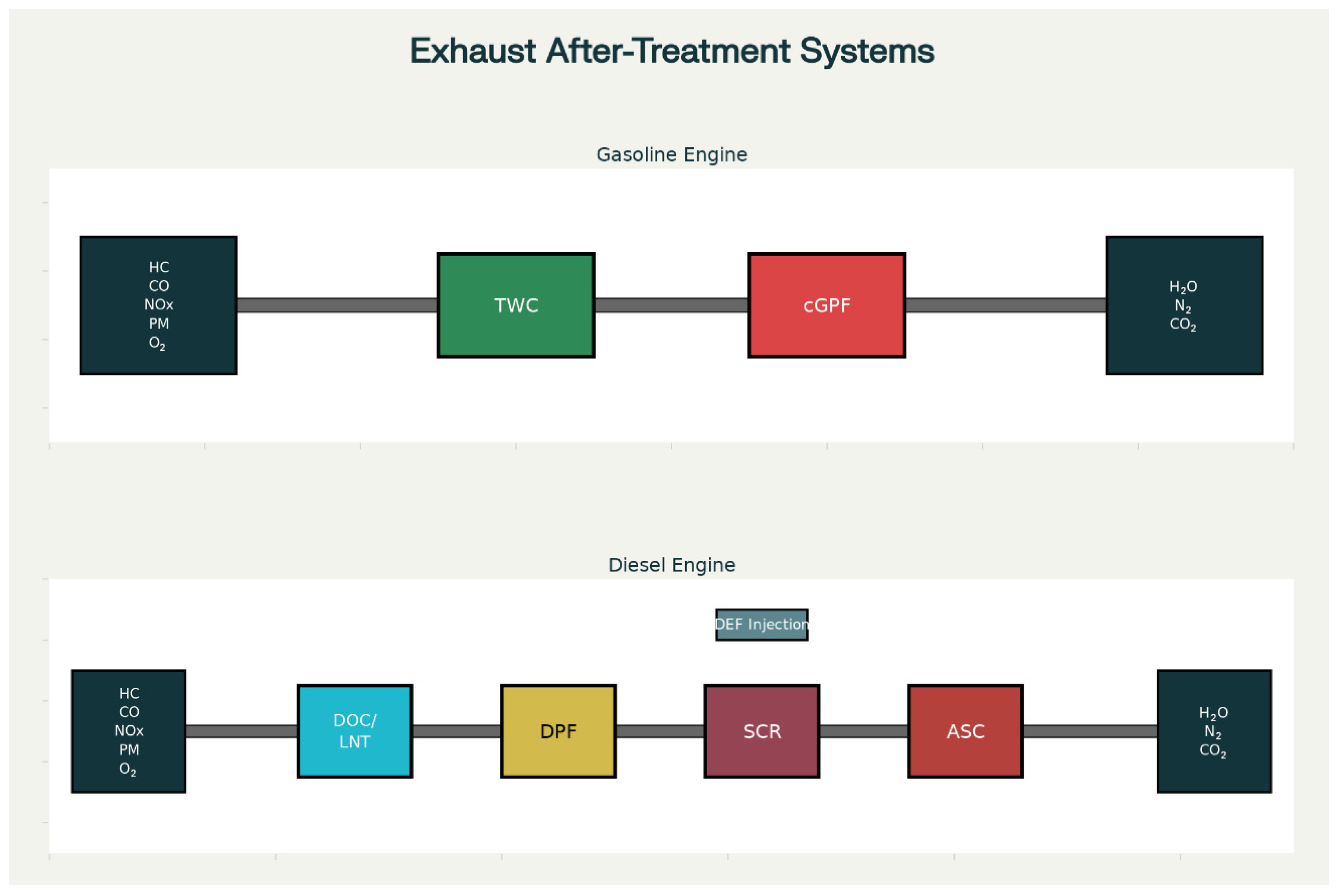
Representative exhaust aftertreatment systems for diesel- and gasoline-powered passenger vehicles demonstrate the complexity of modern emission control architectures. Typical exhaust aftertreatment systems for diesel- and gasoline-powered passenger vehicles are shown in Figure 2.
Figure 2.
Exhaust aftertreatment systems on diesel and gasoline vehicles.
4. Particulate Filter Technology: The System
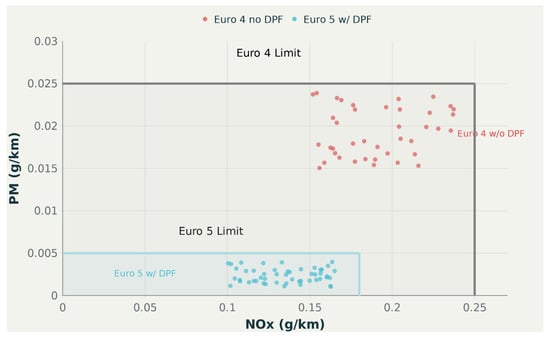
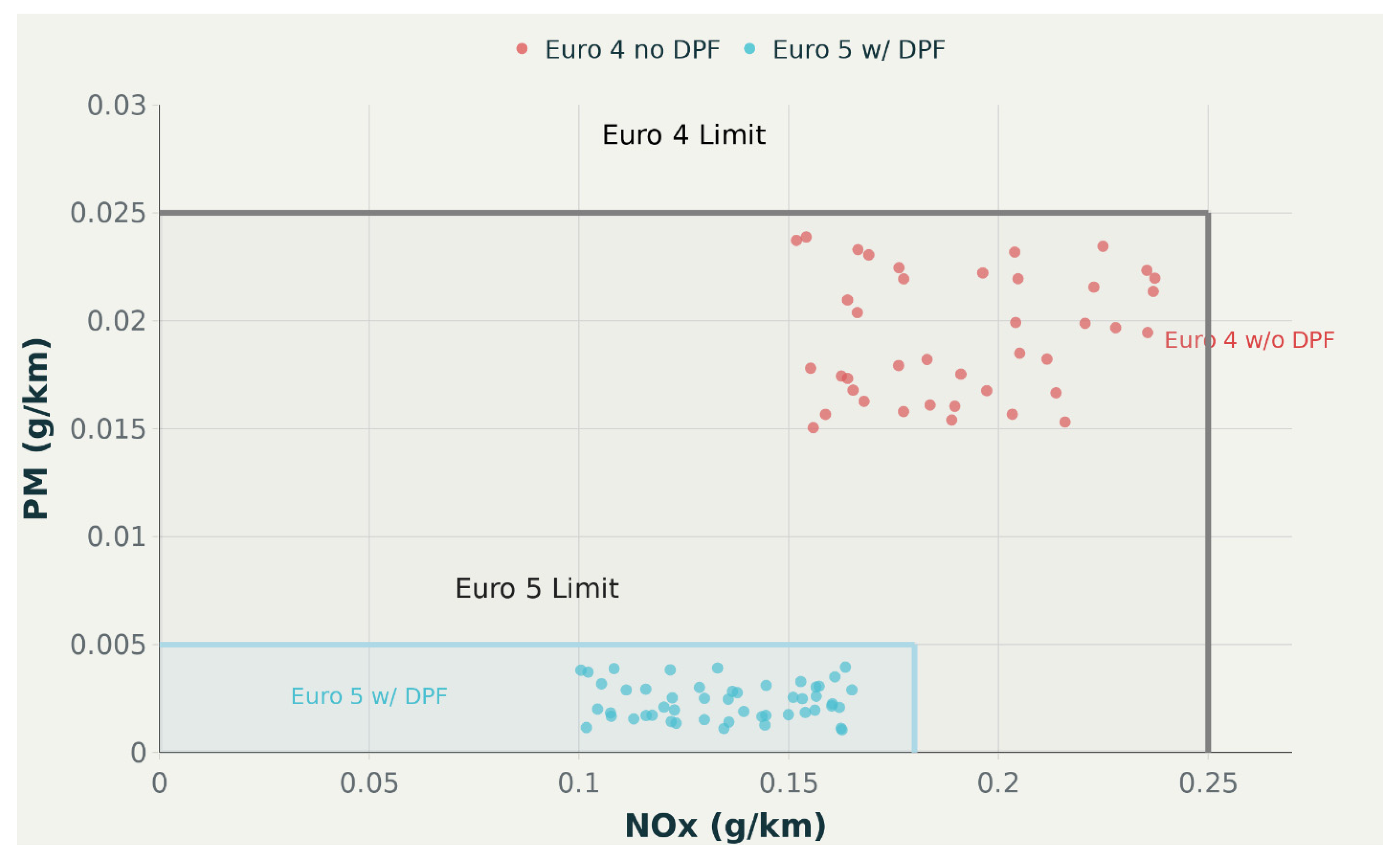
As discussed in the previous section, optimising engine-out emissions as well as integrating optimized, highly efficient aftertreatment technology is the key to achieving stringent emission standards while retaining excellent fuel economy in modern passenger vehicles [22,23]. Euro 5 European emission requirements, effective from September 2009, first led to the DPF technology introduction on diesel vehicles. Figure 3 illustrates the DPF requirements for meeting Euro emission standards for PM [24].
Figure 3.
Requirement of DPF to meet Euro emission standards for PM.
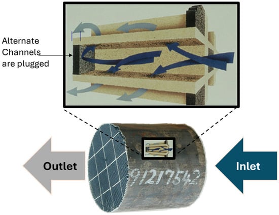
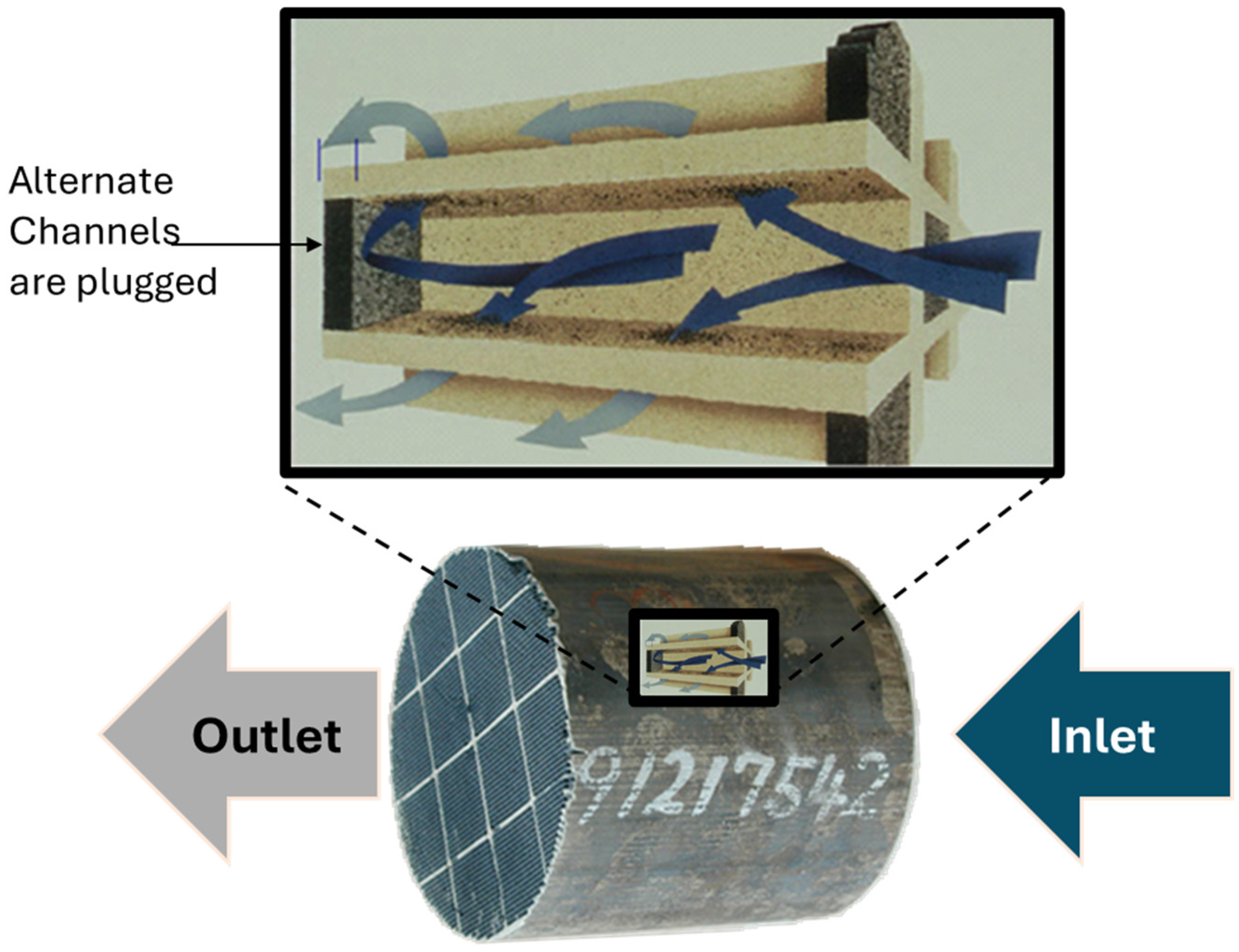
DPF systems typically consist of substrates similar to catalytic converter materials, with individual passages blocked alternately so exhaust gases cannot pass directly through but must traverse the wall structure. This design forces exhaust gas flow through porous walls where soot particles are deposited within wall structures and in cake layers on passage surfaces as shown in Figure 4 [25].
Figure 4.
Exhaust gas flow through a DPF.
In certain applications, exhaust gas temperature and composition enable soot oxidation over operating cycles by NO2 [13,14]. However, in light-duty vehicles with relatively lower exhaust temperatures during normal drive cycles, soot levels increase over time and require removal through periodic filter regeneration. This process is termed ‘Regeneration’ or ‘Regen’ [26]. Periodic regeneration is triggered at variable intervals based on the estimated soot load. Engine controls (throttling, fuel injection timing delays, additional late injection, etc.) raise exhaust gas temperatures typically to 600–650 °C at the DPF inlet to enable regeneration [9,27].
5. Diesel Particulate Filter (DPF) Calibration Challenges: The Problem
DPF system calibration and optimisation presents challenges similar to other exhaust aftertreatment systems. These systems represent among the most complex technologies, with combined engine parameter control being particularly arduous. RDE requirement introduction (incorporating more severe real-world driving conditions) has elevated the challenges to unprecedented levels.
5.1. System Complexity
The particulate filter traps and contains the particulate matter present in the exhaust gas. It also features a catalytic coating, with a similar formulation to that used in the oxidation catalyst, which promotes both thermal and passive filter regeneration. Both the diesel particulate filter (DPF) and the gasoline particulate filter (GPF) have similar functionality except that the GPF may not need as many thermal regenerations as needed by a DPF due to the fact that the engine-out soot from the gasoline vehicles is much lower in most of the operating conditions and the GPF is continuously regenerated due to higher exhaust gas temperatures.
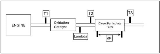
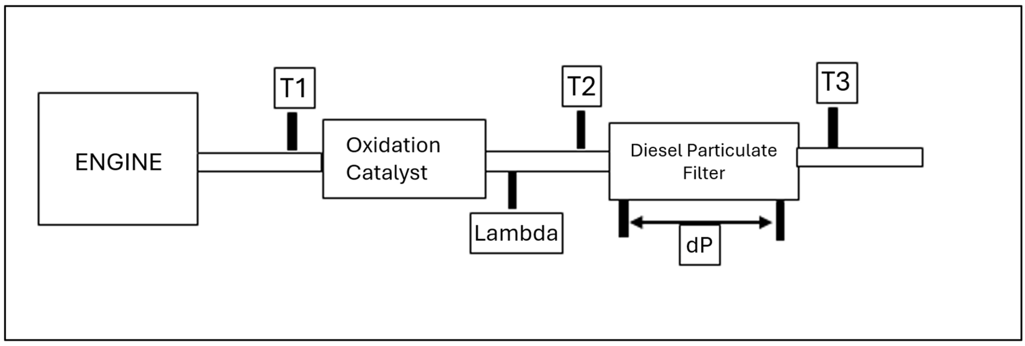
Figure 5 shows the main elements of a particulate filter control system used in a light-duty diesel vehicle.
Figure 5.
Schematic diagram of a particulate filter system.
A lambda (oxygen) sensor is part of the engine air control system that co-ordinates the exhaust gas recirculation system with boost and fuel control. Its output is also used by the particulate filter system to help model the effect of transient events on soot production rates. The temperature sensors (T1, T2, T3) are used by the control system to control temperatures in the oxidation catalyst and the filter within their target temperature ranges during filter regeneration. They are also used to model gas volume flow rates and rates of passive filter regeneration during normal engine operation. The pressure sensor measures the pressure drop across the filter as part of the strategy to measure the soot loading of the filter and this measurement is used in parallel to the ‘open loop’ soot model.
In thermal regeneration, the particulate filters are regenerated by elevating the temperature of the exhaust gas to burn off the carbon. This process increases fuel consumption and engine-out NOx, ages catalysts, and can result in engine lubrication oil dilution (also known as FIO—fuel in oil), so it is beneficial to minimize the frequency of the regeneration events. However, if too much soot builds up in the filter, fuel consumption will increase with increasing back pressure, which may block it entirely, causing the engine to stall, or lead to excessive temperatures when it does burn, with the potential to damage the filter and vehicle [28].
Estimating correct soot levels in the particulate filter in all driving and ambient conditions is a challenging job. The empirical model is based on testbed measurements that often do not represent the real harsh driving conditions. The delta pressure method for soot estimation, which is calibrated against the volumetric flow rate of the exhaust gas, is also not accurate in certain conditions like low engine speeds and very low and very high exhaust temperatures.
5.2. Drive Cycles Complexity—RDE Impact
Despite increasing emission standard stringency, serious shortcomings have emerged in emission control under real-world driving conditions. Studies beginning in 2011 using portable emission measurement systems (PEMS) and remote-sensing techniques quantified unexpectedly high real-world emissions from European diesel passenger cars [4]. Traditional test cycles used for type approval and aftertreatment development failed to capture the full range of engine map operating conditions typical of real-world driving.
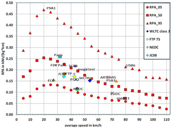
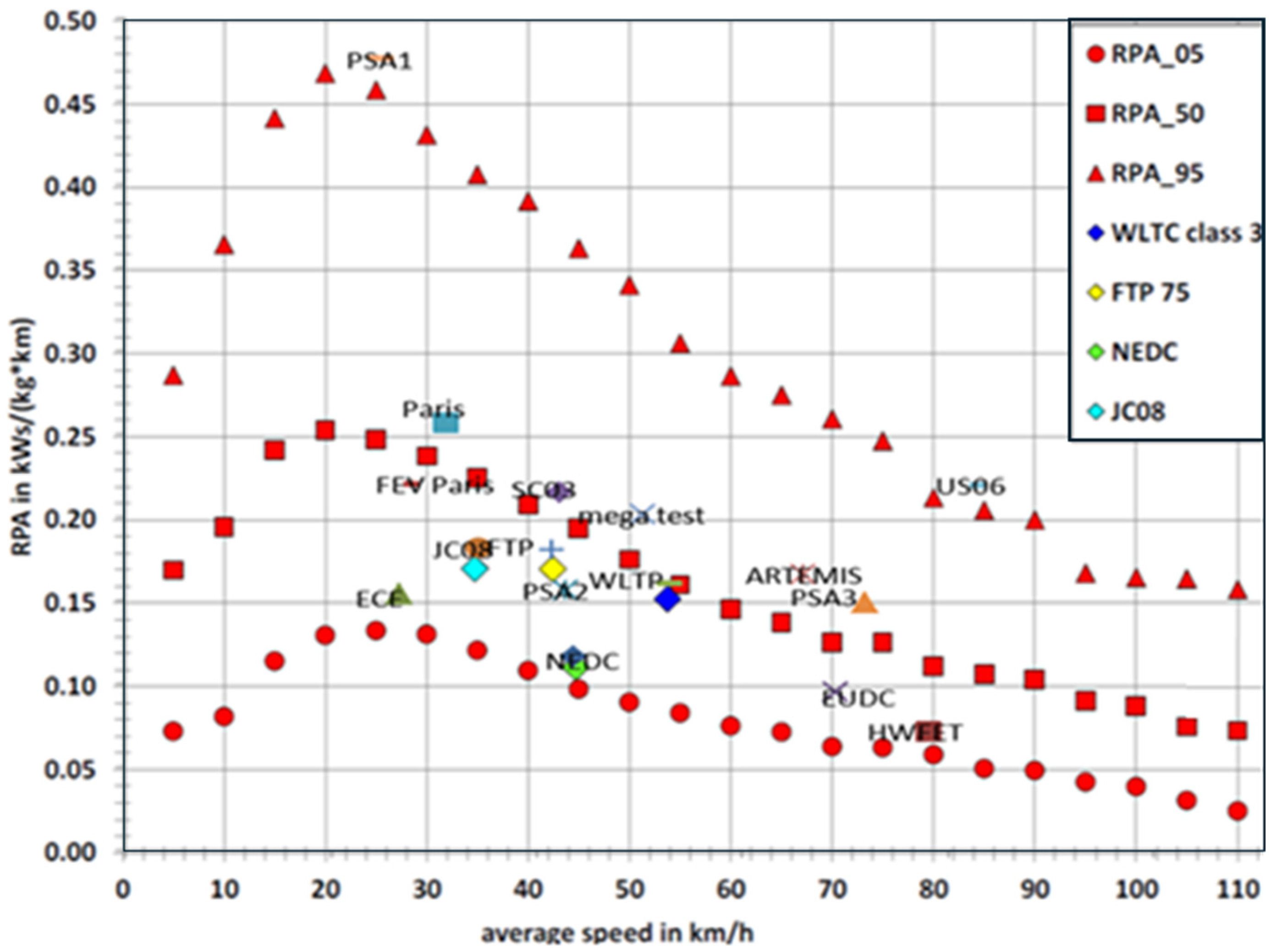
Starting from Euro 6, the introduction of real driving emissions (RDEs) represents a fundamental shift in how vehicles are tested and aftertreatment systems are calibrated. RDE tests measure emissions under actual on-road driving conditions accounting for the natural variability of traffic, road topology, weather, and driver behaviour. Therefore, for emission aftertreatment system control and calibration, substantially broader engine operating condition ranges must be covered to meet current and future RDE compliance. Various known standard drive cycles are shown in Figure 6, where acceleration is plotted against mean speed, which demonstrate the diversity of operating conditions. The RPA (relative positive acceleration) boundaries are defined in the EU regulations [29]. The regulatory boundary conditions for RDE testing include dynamic constraints where valid RDE tests must fall between the RPA_05 (lower boundary) and the VA95 or RPA_95 (upper boundary) lines [29].
Figure 6.
Typical development drive cycles mapped as relative positive acceleration (RPA) vs. average cycle speed.
Relative positive acceleration (RPA) is highest for the mostly transient, and lower for the motorway cycles. Particularly low is the value of RPA for the NEDC [30]. This demonstrates why the NEDC cycle provides insufficient operating condition diversity, necessitating the introduction of RDE testing with its RPA_05 and RPA_95 boundaries to ensure comprehensive aftertreatment system calibration coverage. Using a mix of test cycles that cover a broader range of RDE and RPA operational areas allows broader engine operating ranges to be covered which were often ignored in the past when using only the NEDC or WLTP test cycles for development [31].
6. Theoretical Framework and the Model Development for DPF Soot Load
The first step of the study is developing an open-loop, ECU-orientated soot model that calculates the amount of soot accumulated in the particulate filter based on the operation of the engine and the thermal–chemical behaviour of the specific filter. The model is formulated in discrete time, consistent with series-production engine control units (ECUs), and is implemented as a set of empirical calibratable maps and scalar parameters. Soot accumulation in the filter is described through a lumped mass balance that combines three contributions: steady-state soot production, additional soot formed during transient engine operation, and soot removal via passive regeneration by NO2. Active thermal regeneration is treated as an external event controlled by the ECU; in this work, it is assumed to fully clean the filter when triggered and is therefore not explicitly modeled in the soot mass balance. The following subsections describe the theoretical framework and the model formulation before the individual model elements are discussed in more detail in the later sections. Detailed background on the models in (1)–(4) is found in [32,33].
6.1. Theoretical Framework
The soot load estimator is modeled to be compatible with production diesel ECUs, where computational resources, signal availability, and robustness considerations favour empirical, map-based models over high-order physical-chemical simulations. The soot production and oxidation rates are represented by calibratable look-up tables and curves indexed by standard ECU variables such as engine speed, load, EGR rate, equivalence ratio, and exhaust temperature.
At the core of the model is a lumped-parameter description of the DPF, in which the soot mass stored in the filter, , is treated as a single state variable that evolves according to a discrete time mass balance in (1):
where is the discrete time index, is the model sampling period, is the steady-state soot production rate, is the additional transient soot production rate, and is the soot oxidation rate due to NO2. Each of these rates is obtained from empirical maps and curves calibrated from engine- and vehicle-based measurements.
The steady-state soot production rate is primarily a function of engine speed and load, with separate characterisations for operating conditions with and without EGR. The effect of EGR on soot formation is captured via an EGR-dependent correction that is added to a non-EGR base map. The transient term accounts for short-duration enrichments of the in-cylinder mixture during rapid torque and speed changes, and is formulated as a function of the instantaneous deviation of the measured equivalence ratio from its steady-state reference value and the absolute mixture richness. The NO2-based oxidation term is modeled in three stages: engine-out NOx generation, conversion of NO to NO2 in the oxidation catalyst and DPF, and temperature- and soot-mass-dependent oxidation of soot by NO2 on the filter substrate.
The mass balance and state definition ensure physical consistency, whereas the empirical maps and parameters provide sufficient flexibility to reproduce the observed soot behaviour over a wide range of steady-state and transient operating conditions, including those encountered under RDE cycles.
6.2. Model Formulation
In the implementation, the soot estimator operates at the ECU sampling frequency and uses standard measured or estimated inputs from the engine and aftertreatment control system. The primary inputs are as follows:
Engine speed, n (rpm);
Engine internal torque or load, Tint (Nm);
Exhaust gas recirculation rate, EGR (%);
Exhaust gas temperatures upstream of the oxidation catalyst and DPF (°C);
Exhaust volume flow rate, Vexh (m3/h);
Engine-out NOx emissions (typically mg/s or ppm);
Instantaneous and steady-state reference equivalence ratio, ϕ.
The single dynamic state of the model is the soot mass stored in the DPF, (g), and the principal output is either this mass directly or a normalized soot load value used by the DPF control strategy. Although the production ECU strategy uses a delta pressure-based estimator, the model described here is purely open-loop and does not rely on pressure measurements for its internal state update.
The three terms in the mass balance are realised as follows.
The steady-state soot production rate is given in (2) by
where
- fbase is a two-dimensional map of soot mass flow rate (e.g., mg/s) versus engine speed and internal torque under non EGR conditions;
- fEGR is a two-dimensional map representing the additional soot production attributable to EGR at each speed–load point;
- gEGR is a factor map or scalar function that determines whether EGR is active and, when active, scales the EGR correction according to the estimated EGR rate.
The calibrated parameters in this sub-model are the breakpoints and entries of the fbase and fEGR maps and the entries of the gEGR activation factor map. These maps are populated and optimized using steady-state testbed data and residency weighted optimisation routines, as detailed in Section 7.2.1.
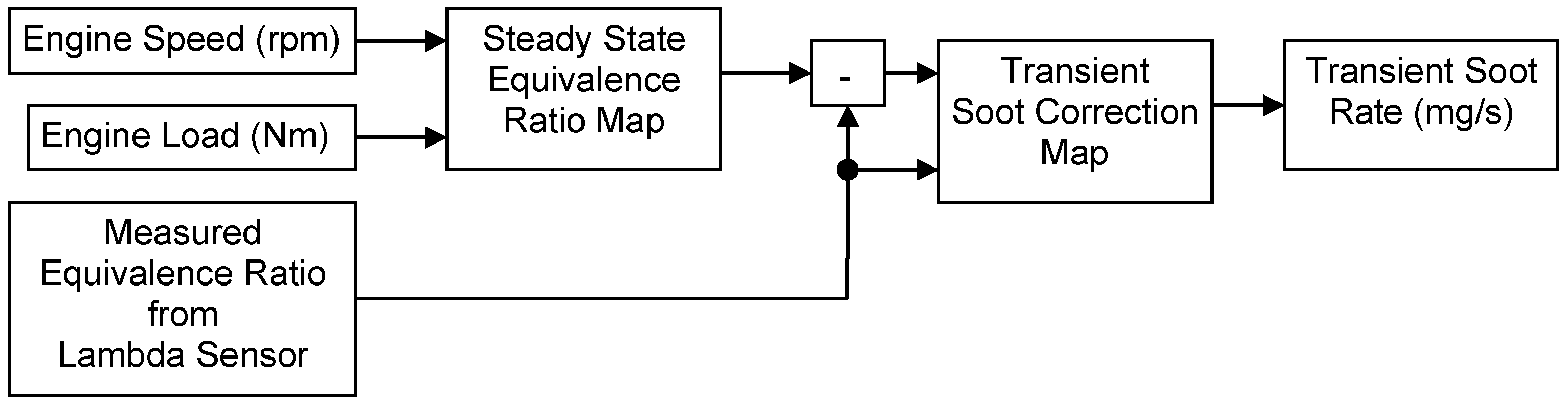
The transient soot is modeled by comparing the instantaneous equivalence ratio derived from the lambda sensor with the steady-state reference equivalence ratio at the same speed–load point. The additional soot rate during a transient is expressed in (3) as
where Δϕ = ϕ − ϕref is the deviation from the steady-state equivalence ratio, and ϕref is the reference value taken from a calibrated steady-state map. The function ftr is implemented as a two-dimensional map generated from families of calibration curves that relate additional soot rate to equivalence ratio deviation for different ranges of ϕref.
The calibrated parameters in this sub-model are the steady-state equivalence ratio map ϕref(n,Tint) and the breakpoints and entries of the transient soot correction map (e.g., additional mg/s of soot as a function of Δϕ and ϕref). These parameters are identified using combined vehicle dynamometer and simulation data, with the calibration and optimisation process described in Section 7.2.2.
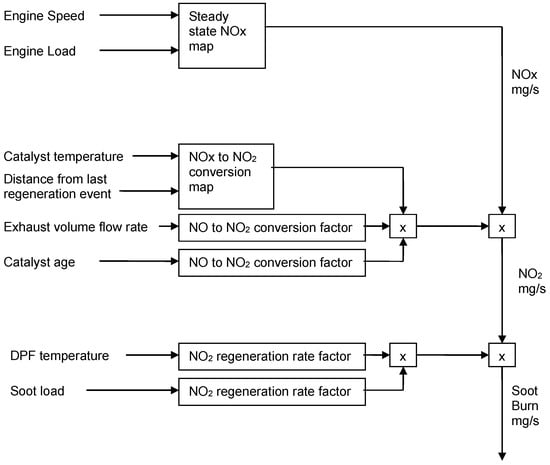
Lastly, the NO2-based oxidation term is formulated in three stages:
- An engine-out NOx map fNOx(n,Tint), providing NOx mass flow rate (mg/s) over the steady-state operating envelope.
- A NO2 conversion ‘make’ surface fNO2(Texh,Vexh), giving the fraction of NOx converted to NO2 across the oxidation catalyst and DPF as a function of exhaust temperature and volume flow rate. Separate surfaces are determined for new and aged components.
- A soot burn rate map fburn(TDPF,mNO2,msoot), relating the soot oxidation rate to DPF temperature, NO2 mass flow through the filter, and current soot loading.
Combining these elements, the soot oxidation rate is given in (4) by
The calibrated parameters in this sub-model are the entries and breakpoints of the engine-out NOx map, the NO2 conversion surfaces for green and aged catalysts, the soot burn rate map, and a small number of scalar correction factors representing the net effect of catalyst ageing.
These parameters are identified from dedicated testbed experiments using new and thermally aged components, combined with repeated weighing of soot loaded filters to determine soot mass loss with time. The methodology for constructing the NO2 make surfaces and soot burn rate maps, as well as the treatment of catalyst ageing, is described in Section 7.2.3.
In summary, the complete model is an empirical, map-based implementation of the soot mass balance equation, configured for efficient execution in automotive ECUs and calibrated using a structured workflow that integrates steady-state engine tests, vehicle drive cycles, and automated optimisation routines. The block diagrams presented in the subsequent sections correspond directly to the functions and maps defined in the equations above and provide a control-engineering view of the same algorithmic structure, providing physical equations for a DPF soot estimation model on a passenger car.
Physical equations for a DPF are given in Appendix A.
6.3. The Soot Model Schematics
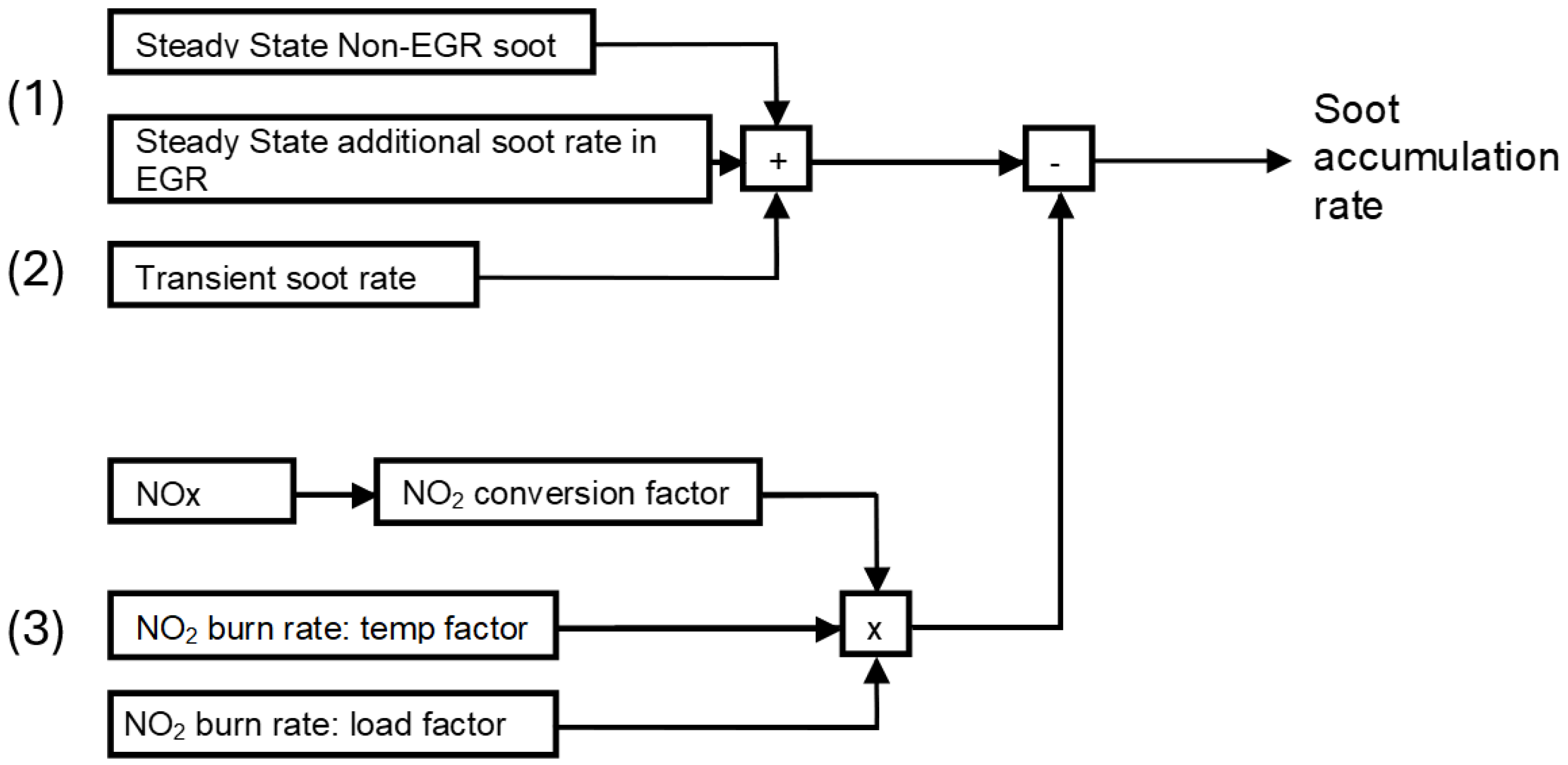
The schematics that make the basis for the model development in the Simulink environment are described in this section. As previously defined, the model has the following three elements which are schematically shown in Figure 7:
- (1)
- The steady-state rate of soot production;
- (2)
- Transient soot production;
- (3)
- The rate of soot consumption by NO2 reduction.
Figure 7.
Functions of the soot estimation model.
6.4. Steady-State Soot
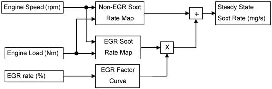
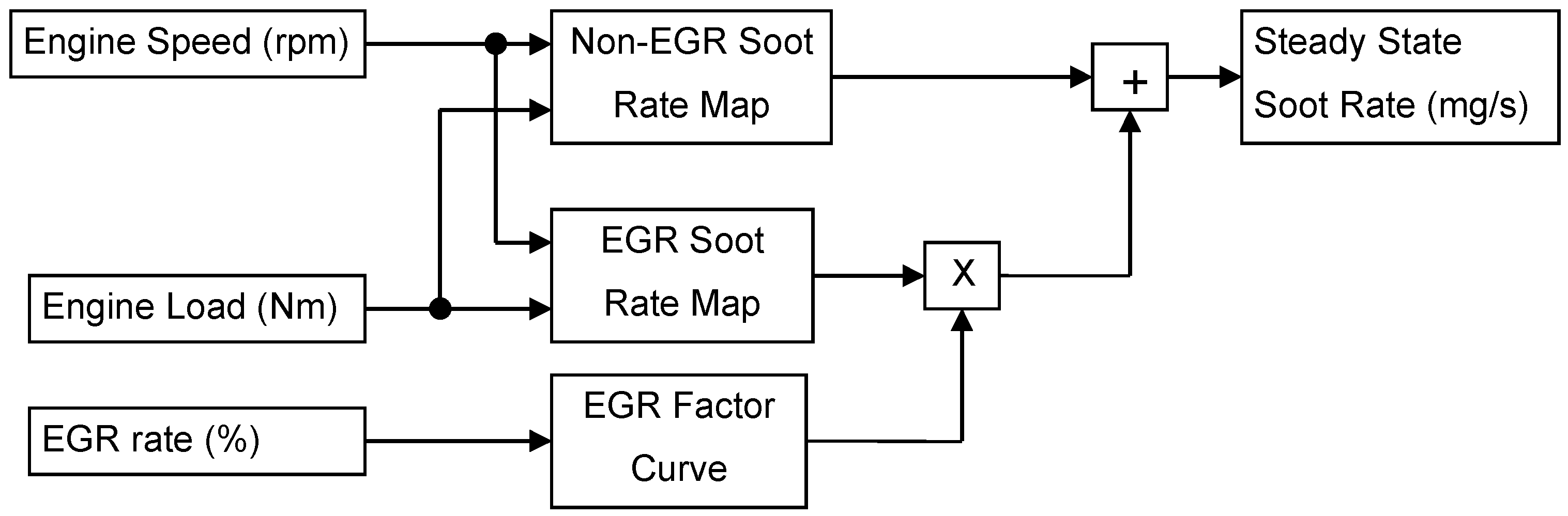
The steady-state maps form the foundation of the estimate of soot production. These are a characteristic of the engine that are developed and fixed during the engine emissions calibration process. Engine development guided by emissions regulation means that through the use of engine condition monitoring and adaption, these characteristics remain broadly constant throughout the life of the engine. The use of EGR to reduce NOx emissions reduces the oxygen content of the charge in the cylinder and as a result tends to increase the amount of soot produced during the combustion process. This difference is accounted for by the EGR soot map whose output is added to that of the non-EGR map when EGR is active.
The base map for the soot estimator is the steady-state map of non-EGR soot production with engine speed and load (see Figure 8). To this is added a correction to the soot rate as the result of EGR. A factor map is used to determine whether EGR is active based on an engine control unit modeled estimate of EGR rate.
Figure 8.
Steady-state soot estimator.
6.5. Transient Soot
During a transient to a higher engine speed, the combustion mixture temporarily becomes richer as the increase in airflow lags the increase in fuel. A reduction in the air–fuel ratio will tend to increase the rate of soot production as the availability of oxygen decreases. Because of this dependency on available oxygen, the amount by which soot rate increases will depend on both the amount by which the mixture is made richer and on the strength of the mixture at the start of the transient event. The significance of this effect, then, is increased when the mixture is already relatively rich, for example, when the EGR rate or engine load is high.
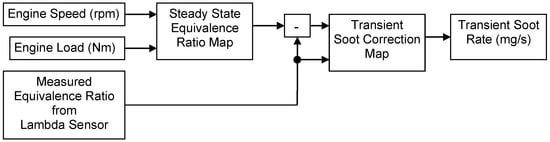
This effect is quantified first by comparing the steady-state equivalence ratio (measure of richness of the air–fuel mixture) with the instantaneous equivalence ratio, derived from the signal from the lambda sensor in the exhaust, to determine the difference (reference Figure 9). The difference in the equivalence ratio is then compared with the total equivalence ratio to determine the additional rate of soot production; so, for a given increase in the equivalence ratio, the increase in soot production will be greater if the total equivalence ratio is higher.
Figure 9.
Transient soot correction strategy.
6.6. NO2 Reduction
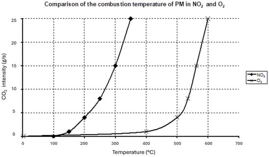
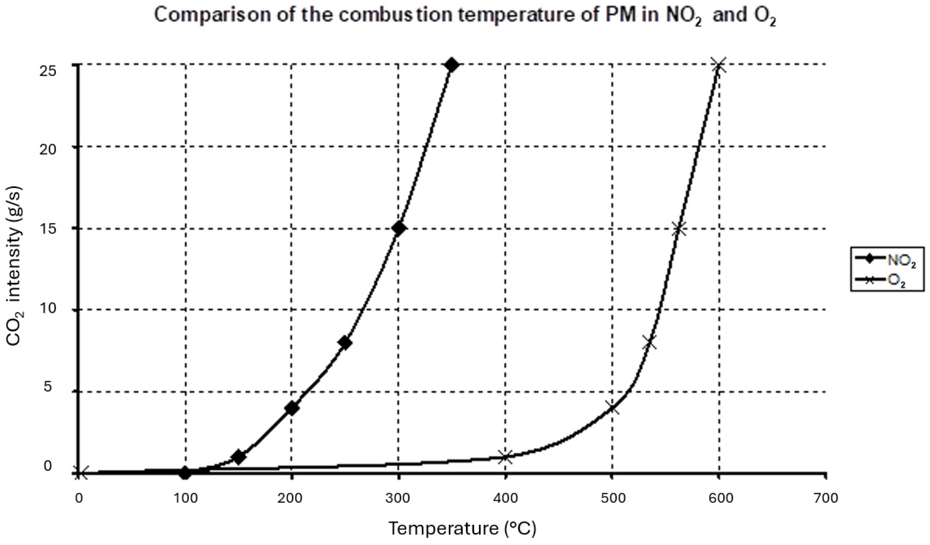
For the soot reduction part, Figure 10 below illustrates how the rate of soot oxidation (also ‘CO2 intensity’) varies with the temperature of the exhaust gas. It shows data from a laboratory reactor, where the temperature was increased while passing an oxidizing gas (NO2 or O2) over a PM sample, and the resulting CO2 (from combustion) was measured. This CO2 was the direct result of the particulate matter (soot) combusting and was monitored using a mass spectrometer [16].
Figure 10.
Soot oxidation rate with temperature.
It can be seen that the onset temperature for soot combustion using NO2 is approximately 200 °C—much lower than the 450–500 °C required for the onset of combustion using O2. This NO2 reaction can be summarized as below:
C + 2NO2 → CO2 + 2NO
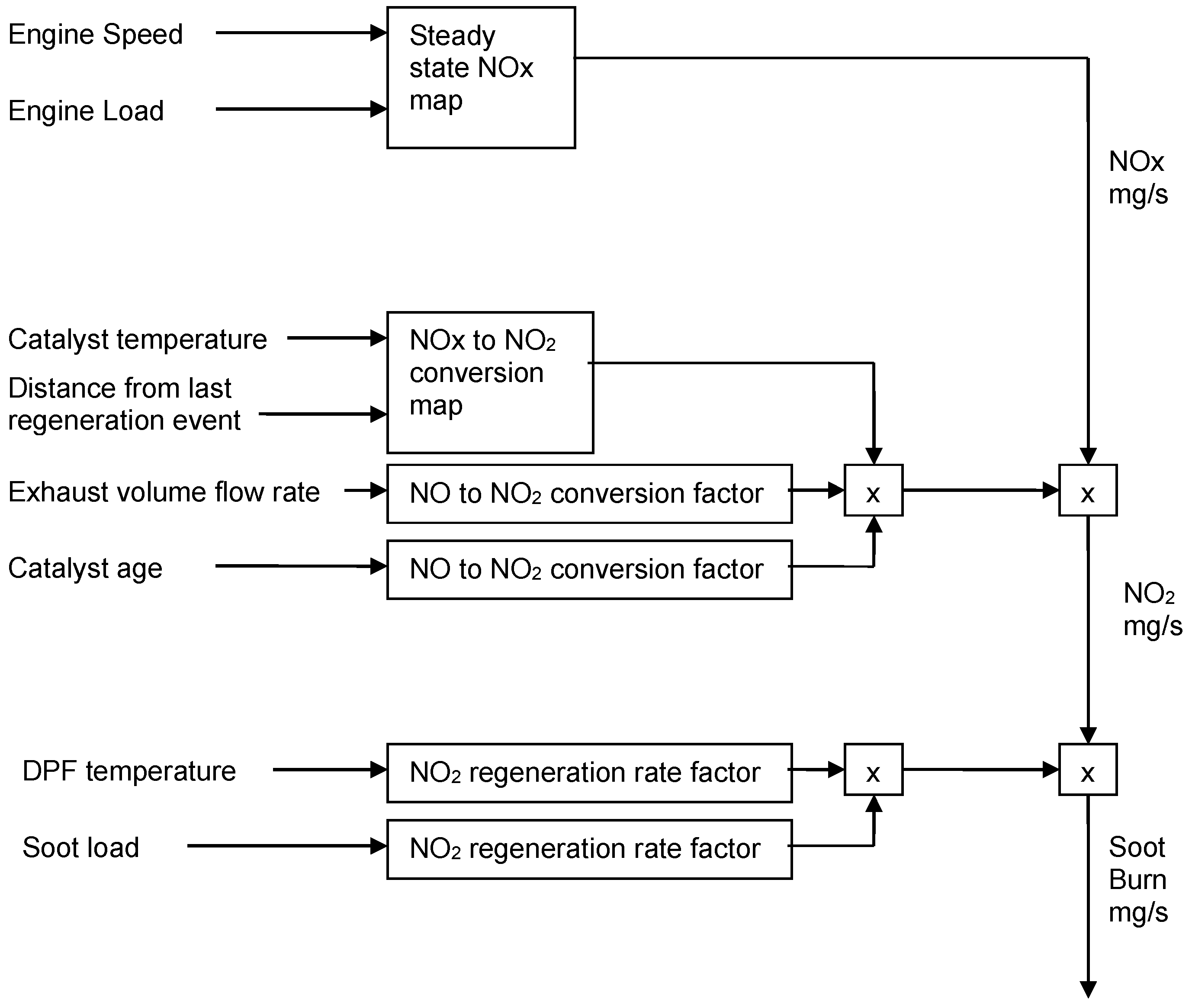
The reaction rate is predominantly a function of temperature and of NO2 concentration. NO2 only makes up 5% to 15% of the total NOx in the exhaust [27] but NO is oxidized to NO2 in both the oxidation catalyst and in the DPF (which has a catalytic coating). The proportion of NOx that is converted to NO2 is a function not only of temperature and residence time, but also of the level of unburned hydrocarbons, and of the condition of the catalyst materials in both the oxidation catalyst and the DPF. The rate at which NOx is converted to NO2 reduces both as the catalyst ages over the lifetime of the component but also as the catalysing material is poisoned by sulphur in the fuel. This sulphur poisoning is reversed at the higher temperatures experienced by the oxidation catalyst and the DPF during thermal regeneration. The strategy employed in the model for soot reduction due to NO2 is summarized in Figure 11.
Figure 11.
NO2 soot oxidation model.
The soot oxidation mechanism is simplified, assuming that NOx emissions from the engine consist solely of NO, that NO is converted to NO2 only in the oxidation catalyst, and that only NO2 oxidation of soot occurs in the particulate filter. In practice, for example, NO2 does constitute a small proportion of the engine NOx emissions and NO is also oxidized to produce NO2 in the DPF. However, here in this model, the focus is on the soot burn rate, which is effective in a small temperature and soot load window, and mostly only available at the high NO2 conditions. So, the above assumptions are suitable for this purpose.
7. Testing, Simulation, and Optimization of the Soot Load Model
To calibrate and optimize the model, a methodology was deployed which consisted of engine- and vehicle-based testing supported by Matlab R2023b scripts, Simulink simulations, and automated optimisation routines. New and thermally aged oxidation catalysts and particulate filters were sourced for testing so that the overall ageing effect of the catalytic coating can be determined over the service life of the system. All the particulate filters used were baselined by heating in an oven to drive off volatile compounds such as binders used in the manufacturing process and to condition the matting located between the filter material and the can. The new green catalysts and filters were also conditioned by running the components through two active regeneration cycles on the testbed. The data were collected from the engine testbed, vehicle dynamometer, and emissions measurement equipment using the AVL data acquisition system. The test system comprised an EU6d compliance 2.0 L hybrid diesel engine with a high-pressure common rail electric fuel injection system of Bosch.
7.1. Engine Tests
Data have been collected from engine development testbeds that have the measurement and control systems in place that allow data to be collected of a quality that is suitable for emissions development and certification test work. The main characteristics are that the testbed is capable of holding a stable engine speed and load at all test points over the range of operation, that the engine temperatures (fuel, oil, coolant, inlet air, intercooler, etc.) can be set and held at reference conditions, and that support instrumentation is available to measure NOx, CO, CO2, smoke emissions, temperature, and pressure along with engine electronic control unit (ECU) parameters.
Mapping tests are automated; the speed and load are set and held constant; a data log is taken once the engine has stabilized on condition and then the speed and load are moved to the next site. Testbed and engine control unit parameter measurements are averaged over 30 s.
7.2. Vehicle Tests
A number of standard test cycles, combined in different ratios to characterize a range of driving styles from average through to extreme, are used in developing calibrations. A selection of these cycles has been adopted for this task, each of which is run on a chassis dynamometer in an emissions laboratory. These log data are at a frequency of 1 Hz for emissions (including NOx, CO, CO2, unburned hydrocarbons, and soot) and dynamometer parameters (load, speed, etc.).
An accurate measurement of the total mass of soot emitted over the test is made by passing a continuous sample of the exhaust gas through filter papers which are weighed before and after the test. This is important because although an MSS is used to measure soot emissions in real time, the results are subject to error due to moisture, temperature, dilution inaccuracies, and other impurities. The measured soot mass can be used as a reference to correct the MSS soot measurement taken over a complete cycle.
Engine parameters are taken from the engine control unit and logged separately. Test preparation, execution, and data collection are all carried out to standard procedures set out in the vehicle certification testing.
7.2.1. Steady-State Calibration
Full engine maps that cover the complete speed–load operating envelope of the engine are run at regular intervals during an engine development programme as the emissions calibration and hardware mature. This, as well as providing the source of the raw data required to populate the steady-state maps, also highlights the necessity to develop methods and tools that simplify the task so that it can be repeated a number of times within this and future development programmes. In this study, at a high level, there are three variables with engine speed and load that need to be determined from the steady-state mapping:
- The rate of engine-out soot emissions with and without EGR operating to calibrate the base soot maps;
- The engine measured equivalence ratio with EGR running to develop the reference condition map for transient soot estimation;
- Engine-out NOx.
In typical engine calibration applications, the objective of engine mapping is to generate smooth maps with minimized gradients without diverging too far from the optimum fit for accuracy. This is to reduce the risk of instability and poor driveability that is associated with ‘spiky’ maps or maps with high gradients. The approach is therefore to smooth the data using equally-spaced breakpoints covering the operating range as a starting point, and then an iterative process of adjusting to attempt to improve the fit to the data. This application, however, is a passive system intended to monitor and record the accumulation of soot, so the emphasis is on optimising the accuracy of the estimate rather than generating smooth maps for stable, predictable engine operation.
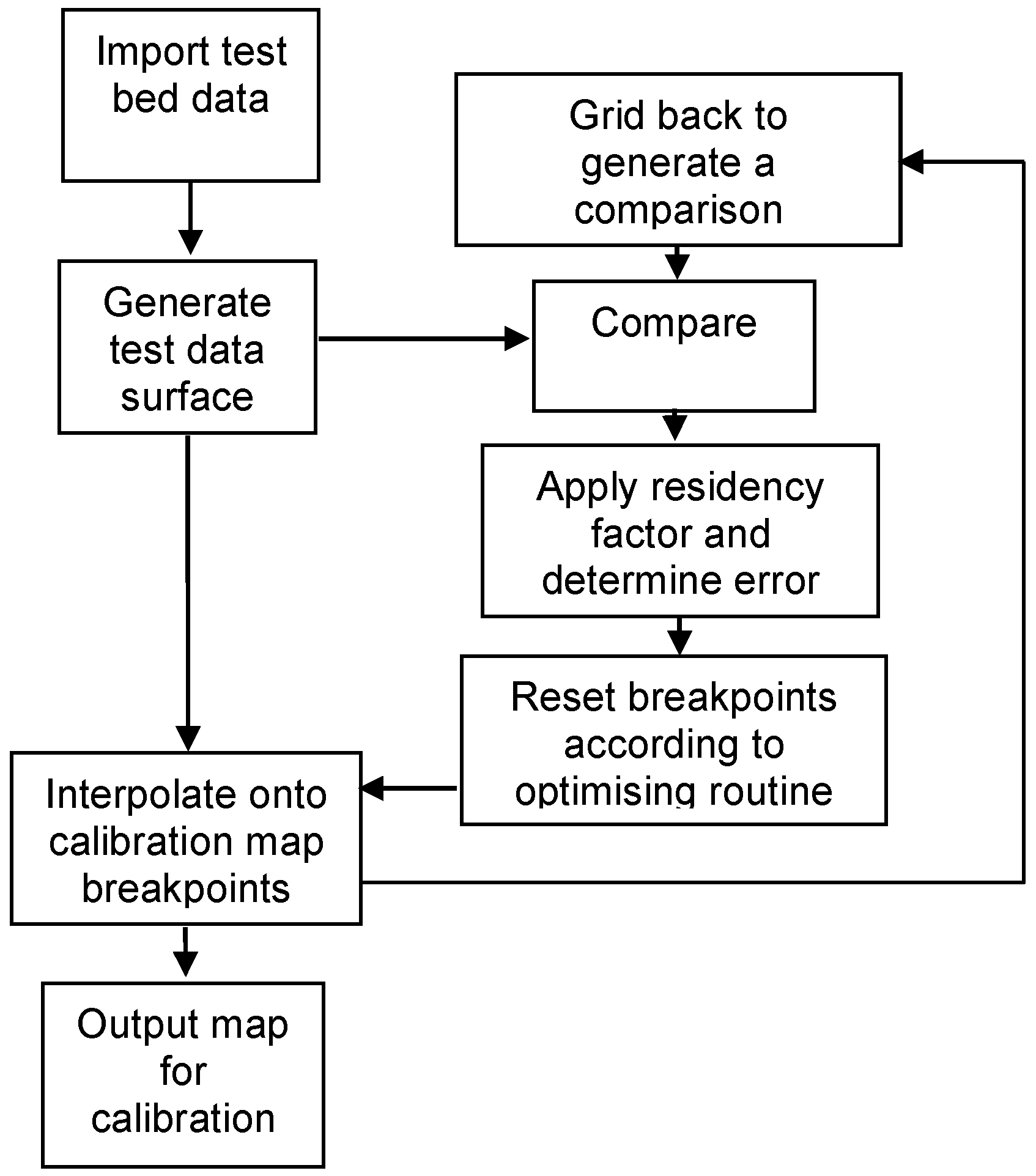
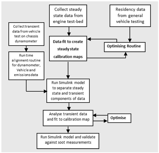
The problem is that there is a complex range of features and gradients that cannot be entirely represented with the low-resolution maps at our disposal that can be practically used in the ECU and the simulation model. The approach is therefore to fit the maps to the data by adjusting the breakpoints such that the error over the operating envelope is minimized. To accomplish this, an optimising routine has been written that attempts to minimize the differences between the measured data and the output from the maps used in the model. This is illustrated in the flow diagram (Figure 12).
Figure 12.
Optimization of steady-state maps.
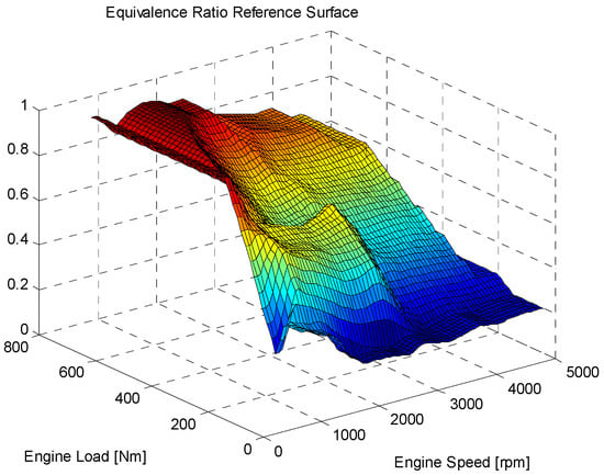
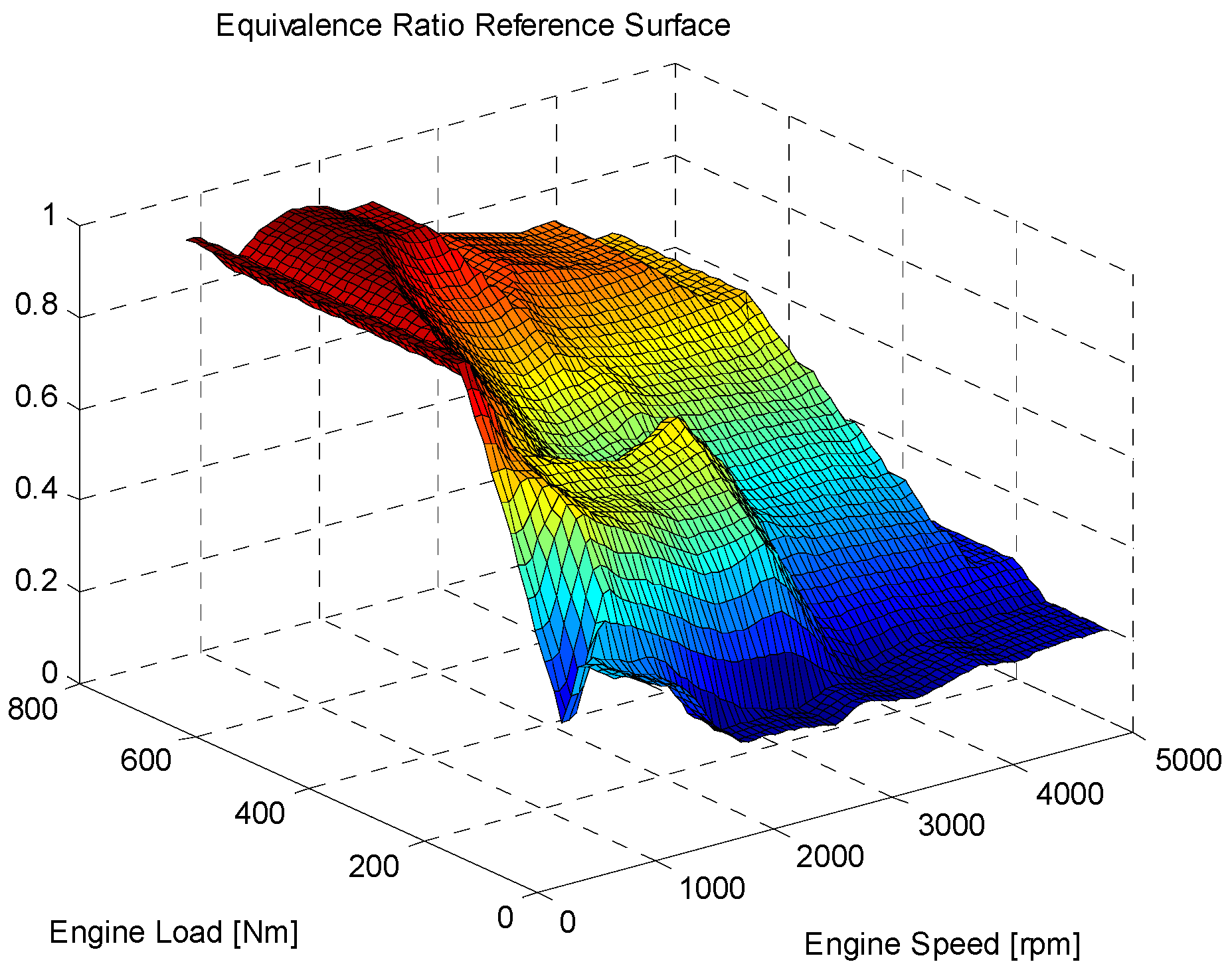
Testbed data are imported and used to generate a data surface (Figure 13). This allows data that are taken during an engine mapping exercise at constant brake torque points to be analysed with respect to constant ‘internal’ torque. Internal torque is the ECU-calculated indicated torque, used as a calibration map axis, which does not have a linear relationship with the brake torque.
Figure 13.
Reference data surface for steady-state equivalence ratio.
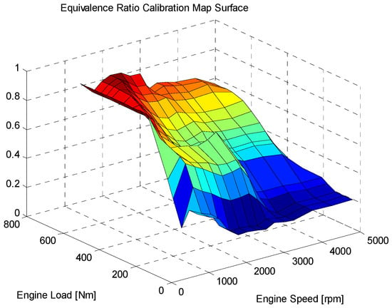
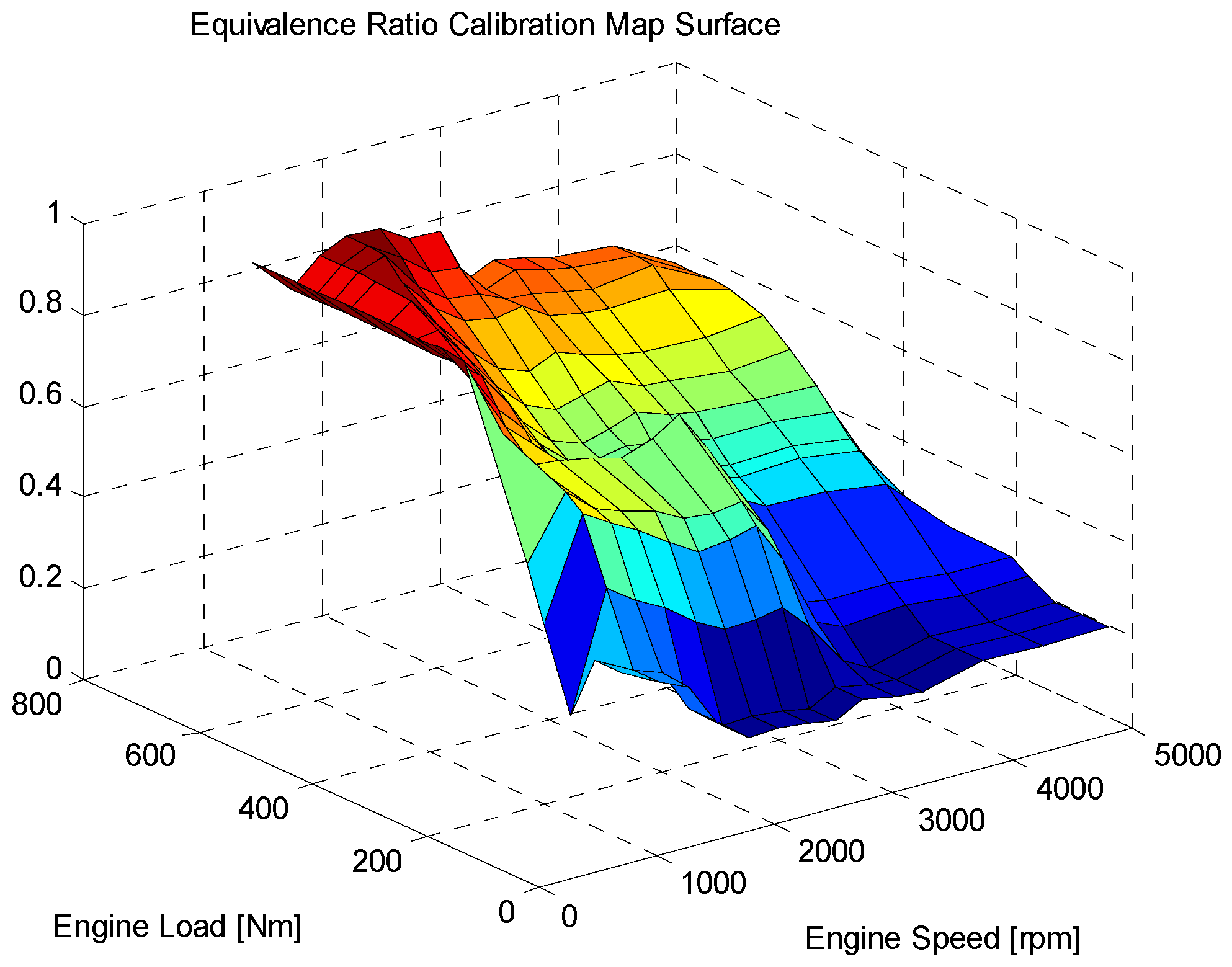
The data surface is mapped onto the calibration map (within the model) by interpolation. This generates a provisional calibration map (Figure 14). In the working calibration, the output of a map is determined by straight line interpolation of the operating point with respect to the map breakpoints. So, interpolation is used again to grid data from this provisional calibration map back onto the axes of the original data surface. The difference between these two surfaces then represents the error between the output of the calibration and the reference data.
Figure 14.
Calibration map surface for steady-state equivalence ratio.
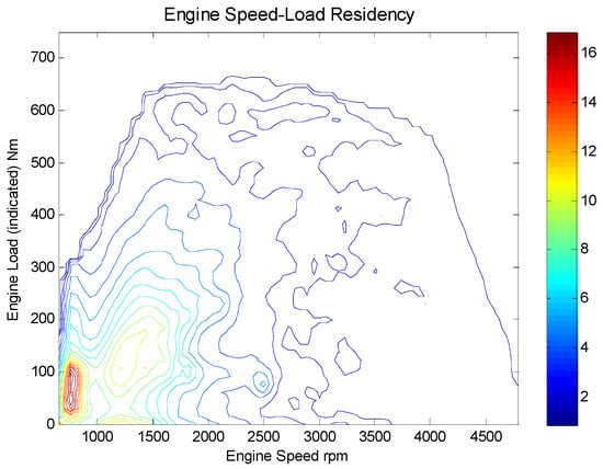
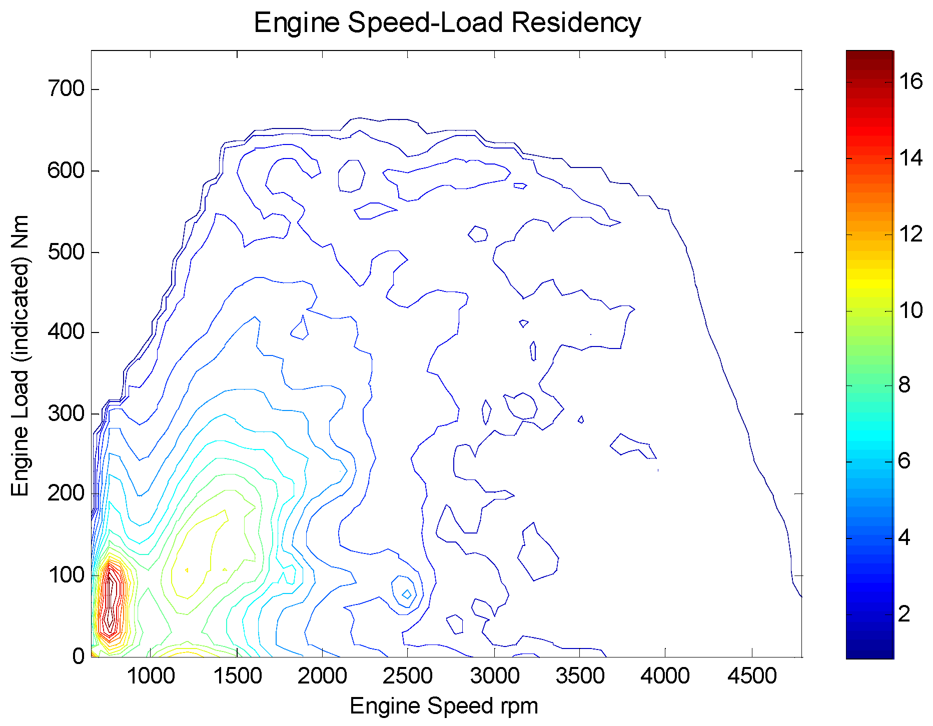
However, a significant area of a rectangular map falls outside the normal operating envelope of the engine, whilst within the operating envelope the proportion of time spent at the various speed–load conditions, the residency time, varies significantly. To account for this, a weighting factor is applied to the calculated error. The weighting factor consists of two parts: the first is a mask where all points of the surface outside the operating envelope are set to zero, and those inside are set to one. This ensures that the error is considered anywhere that the engine has the potential to operate. The second is a factor based on vehicle engine residency data. These data have been assembled from a selection of sources: chassis dynamometer tests, pre-defined vehicle road drive cycle tests, and from random vehicle tests on roads and test tracks where speed–load data have been collected. A routine has been written to convert speed–load data into smoothed residency factor data surfaces to the same dimensions as the testbed data surfaces; a contour plot of the result is shown in Figure 15.
Figure 15.
Smoothed contour plot of engine speed–load residency.
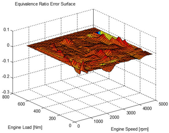
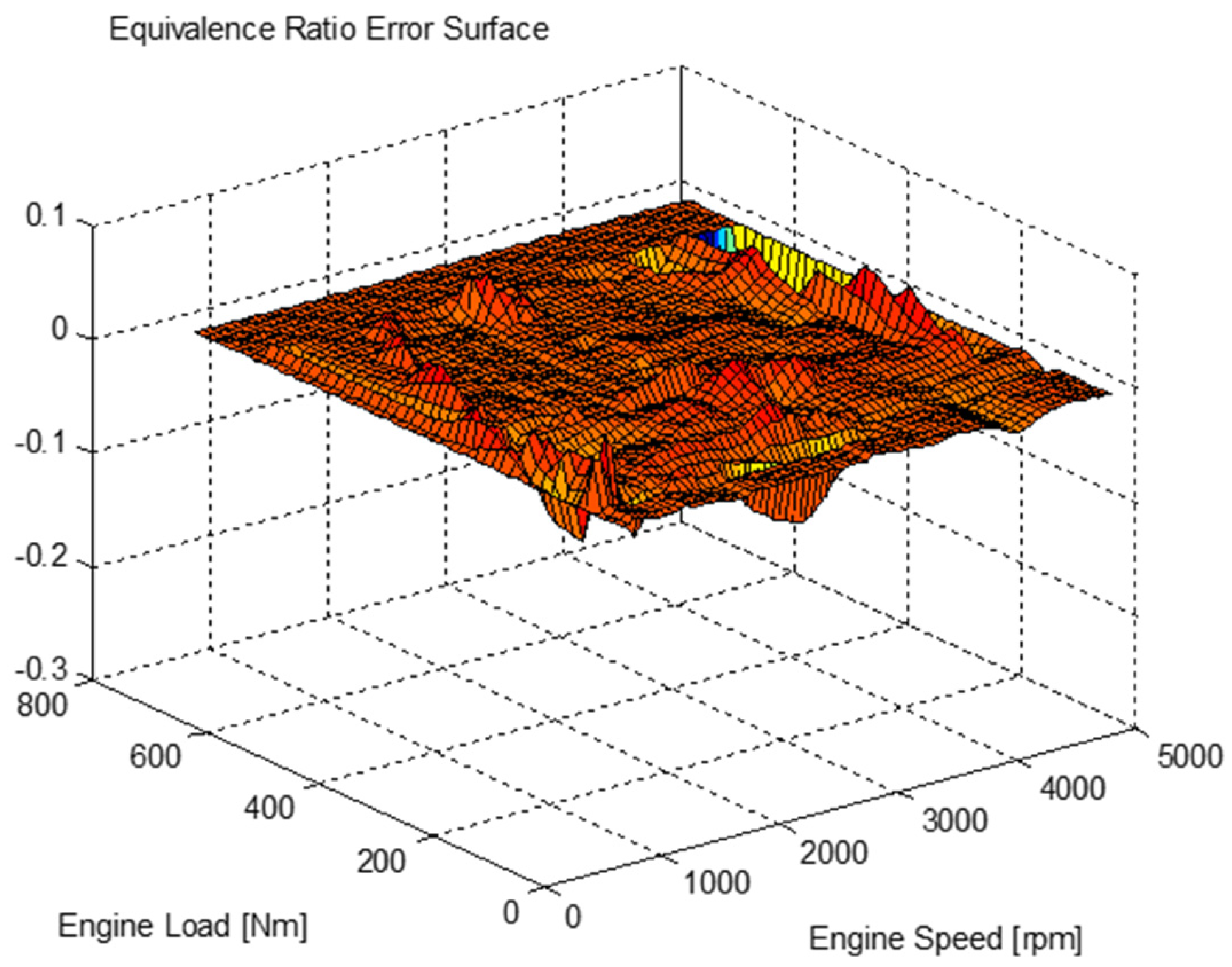
This surface is added to the mask and is multiplied by the difference surface to give an error surface (Figure 16). This mask map representing the residency is multiplied to select the data in the operating conditions which are likely to exist, i.e., where the vehicle operates.
Figure 16.
Error surface for equivalence ratio calibration map.
The cost function for the optimising routine is then a summation of the elements of this error surface. This is performed in two ways: a straight sum and a sum of the square of the error. Squaring eliminates the negative error points and allows the overall magnitude of the error to be assessed, but the simple sum indicates whether the estimated result over the operating cycle is likely to be above or below that indicated by the reference data. This is useful in deciding whether to accept or reject a solution generated by the optimizer; for example, in an estimate of soot production, for safety a slight overestimate may be preferable, whilst for NOx an underestimate is better.
The optimizer works by repeatedly altering each breakpoint in turn by a specified increment and calculating the cost function until the error increases. The increment is then reduced, and the process is repeated. The starting values for the breakpoints, the size of the initial incremental changes, and the number of iterations are all variables that influence the solution. The error plots and the two error values are used to identify the regions of the surface where the errors are generated and so act as a guide in resetting the starting conditions or in deciding the acceptability of the solution.
7.2.2. Transient Soot Correction
The transient soot production model is based on measuring the difference in the oxygen concentration (derived from the lambda sensor) in the exhaust during steady state with that which occurs during a transient event and then relating this difference to the additional rate of soot production during that manoeuvre. The calibration of the transient soot correction is performed in three stages:
- (1)
- Vehicle tests on a chassis dynamometer to collect emissions data for a range of drive cycles.
- (2)
- Run a Simulink model of the soot estimator model over these drive cycles, to calculate the steady-state element of soot production and the deviation of the instantaneous equivalence ratio from the steady state.
- (3)
- Compare the steady-state soot and the measured soot production to determine the transient element of soot production and calibrate against the deviation of the equivalence ratio from the steady state.
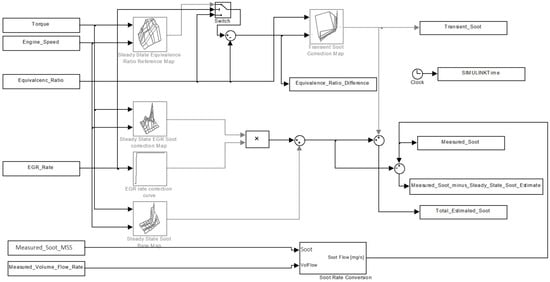
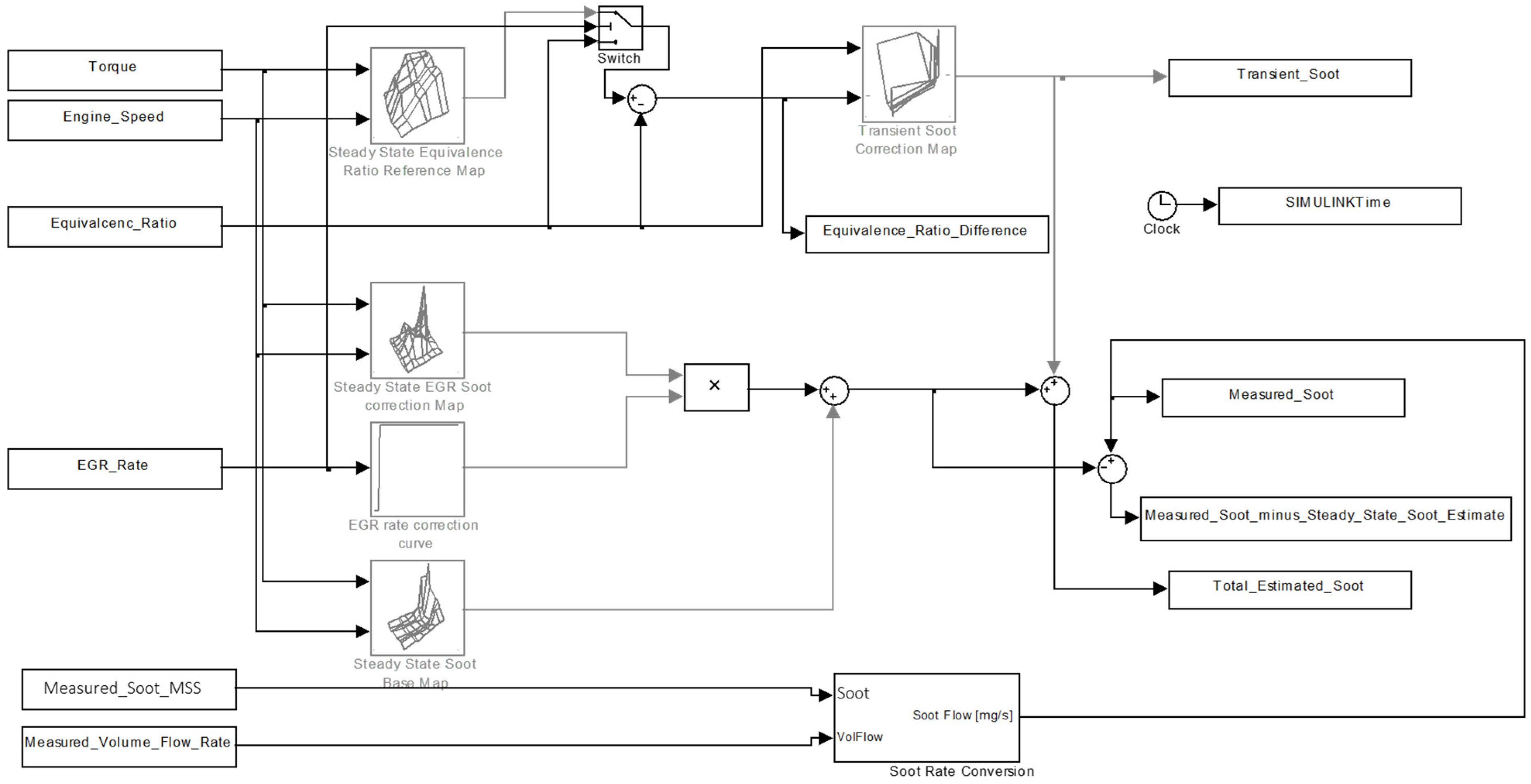
The test data, specifically the variables of engine speed and load, EGR rate, equivalence ratio, measured MSS soot rate, and exhaust volume flow rate, are used as the input variables for the Simulink model as shown in Figure 17.
Figure 17.
Simulink model of the transient soot correction strategy.
The other pre-requisite to run this Simulink model is that the steady-state maps for the soot and equivalence ratio have been calibrated. The first run of the model generates a dataset of the differences between the steady-state and estimated values for soot production and the equivalence ratio. These two variables, with the corresponding total measured equivalence ratio, are used to generate and optimize the transient soot correction map.
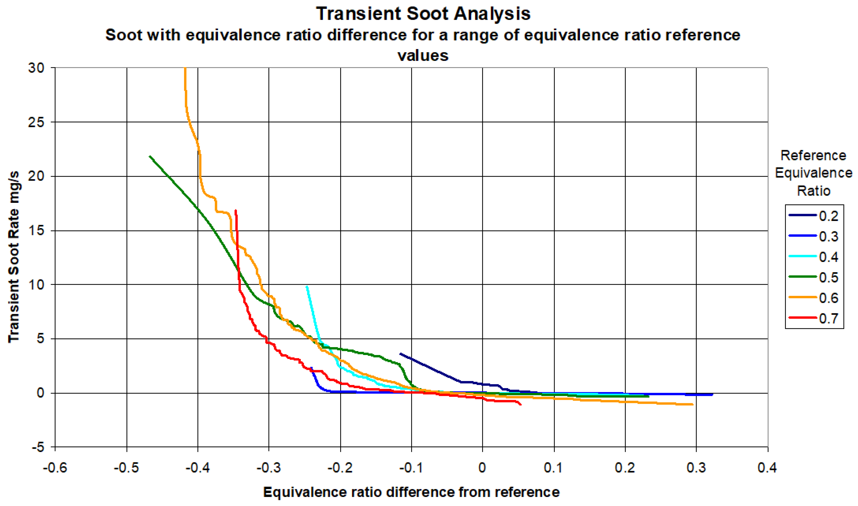
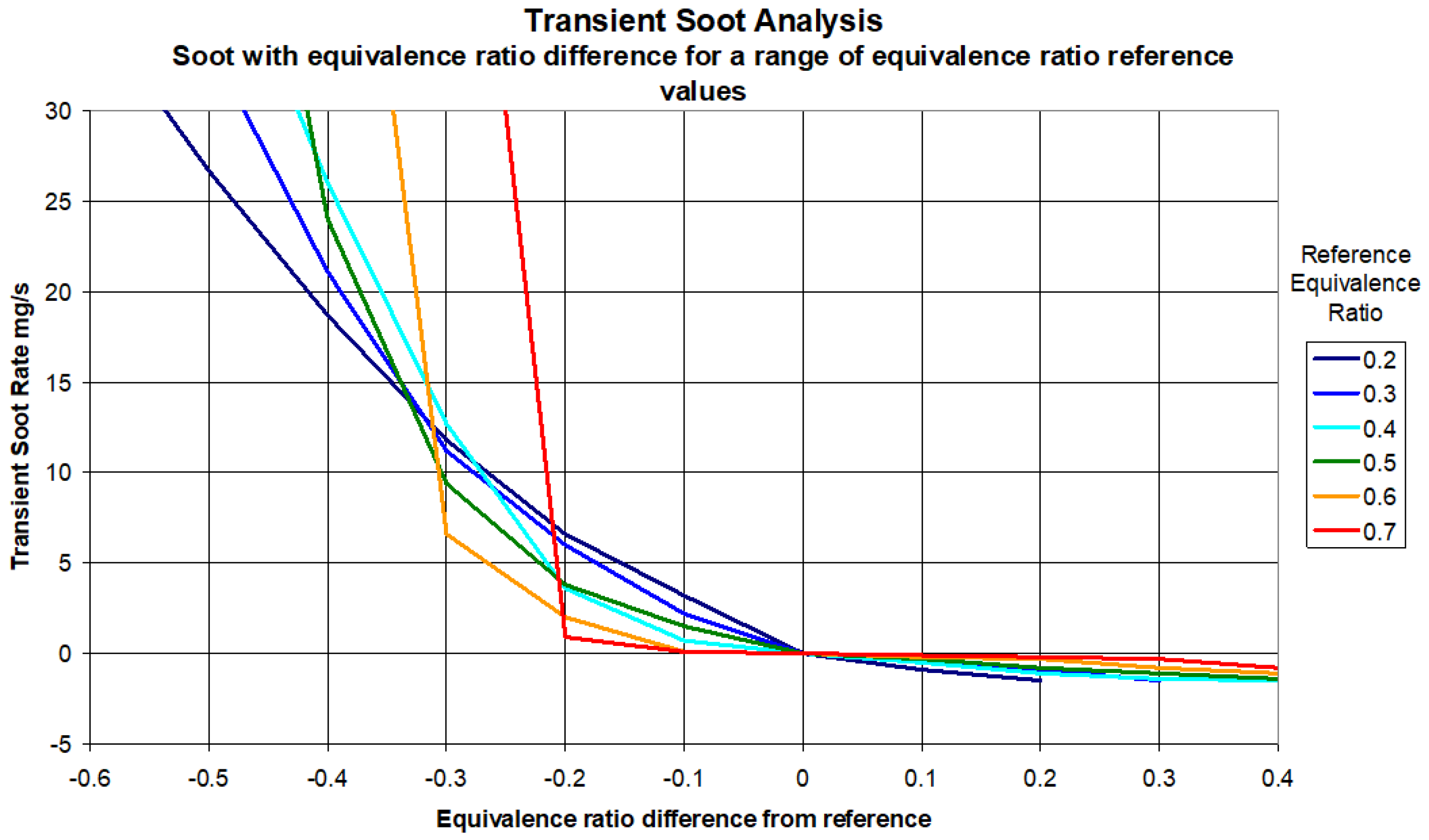
In the optimization routine, the dataset has been sorted and divided according to the reference equivalence ratio. Within each of these divisions, the datasets for equivalence ratio difference and for transient soot were sorted independently in order to de-couple the magnitudes from time. These are plotted in Figure 18 and used as a guide to generate the set of curves plotted in Figure 19.
Figure 18.
Transient data plotted according to reference equivalence ratio.
Figure 19.
Transient soot correction curves fitted to transient data plots.
The transient correction curves were then used to back calculate the transient soot values for the measured equivalence ratio and equivalence ratio difference to populate the transient correction calibration map with first fit values of the right magnitude and following the correct trends. Re-running the model allowed the transient correction map to be trimmed to correct for errors in the curve-fitting process and also to correct for errors between MSS and filter paper measurements for soot.
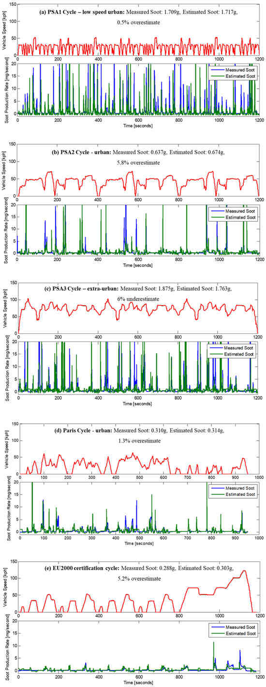
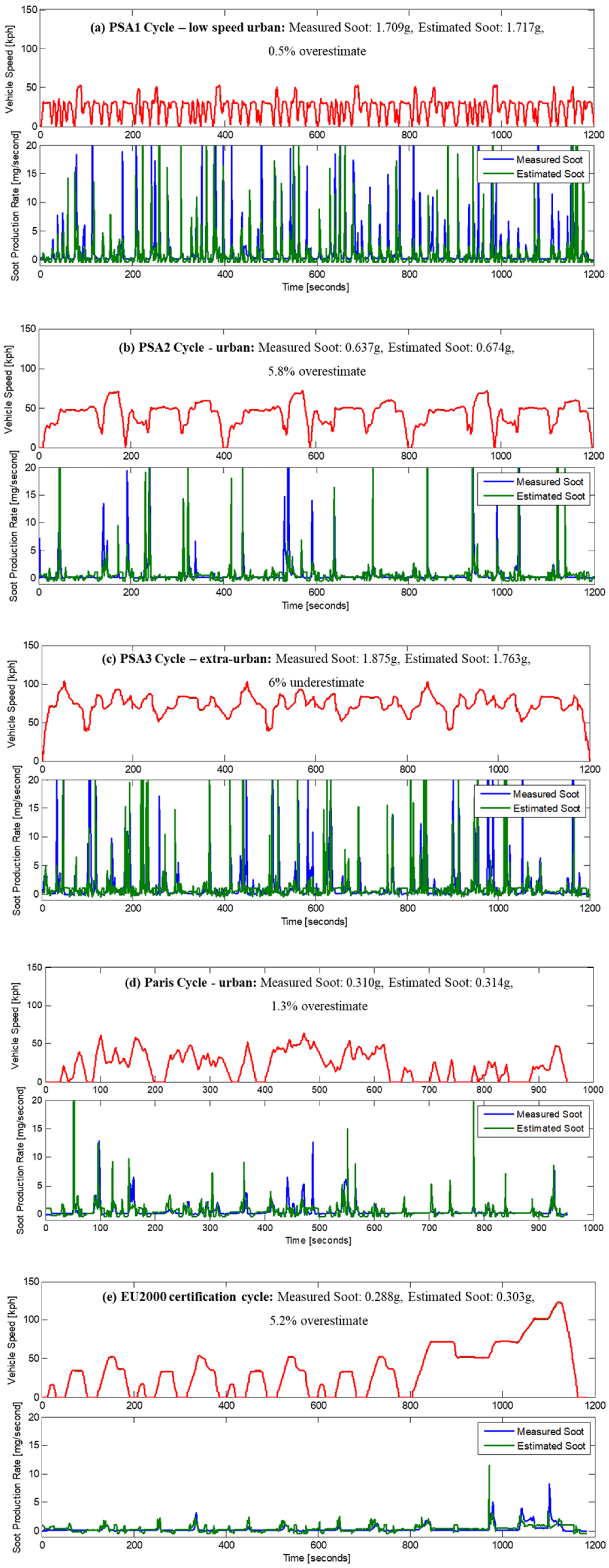
Once the transient soot correction map has been optimized, the model was re-run as a validation exercise to evaluate the performance of the calibrated soot model in estimating the rate of soot production. A graphical representation is given in Figure 20 for individual cycles, which shows an estimate of the soot emissions for all standard drive cycles within 6% accuracy.
Figure 20.
Measured and estimated soot emissions over individual cycles.
7.2.3. NO2 Mechanism for Soot Oxidation
The rate of the passive regeneration of the filter soot by means of the NO2 mechanism, described in Section 6, is modeled in three stages:
- (1)
- Estimate the engine NOx emissions with respect to engine speed and load.
- (2)
- The rate of NO conversion to NO2 with temperature and volume flow rate.
- (3)
- The rate of soot mass reduction in the filter with filter temperature, NO2 flux, and soot mass.
7.3. Engine-Out NOx
The steady-state mapping and analysis of the engine-out emissions to produce the optimized calibration maps are described in Section 7.2.1. However, for simplification, there is only one map available in the strategy for engine-out NOx. So, this map is particularly optimized for non-EGR conditions because when EGR is active NOx emissions are very low and hydrocarbons (which tend to reduce the conversion efficiency of NOx to NO2) are relatively high. The assumption has been made that in the EGR operational conditions, passive regeneration is not significant.
7.4. NOx to NO2 Conversion
The rate at which engine-out NOx is converted to NO2 has to be characterized with respect to the temperature of the exhaust gas at the entry to the oxidation catalyst, and to the volume flow rate of the exhaust gas. A specific testbed experiment has been devised to determine the rate of NOx to NO2 conversion. The testbed emissions analyser (HORIBA MEXA-7000 series, HORIBA UK Limited, Northampton, UK) is normally set up to measure the NOx concentration, but it can also be switched to measure NO. For this experiment, the apparatus was configured to take measurements of both NO and NOx at each speed–load test point. The assumption is made that oxides of nitrogen other than NO and NO2 are insignificant so, although NO2 cannot be measured directly, it can be inferred by difference. These tests were carried out with both new and aged components so that the overall effect of catalyst ageing can be determined over the service life of the system.
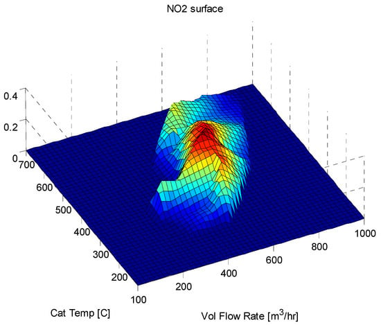
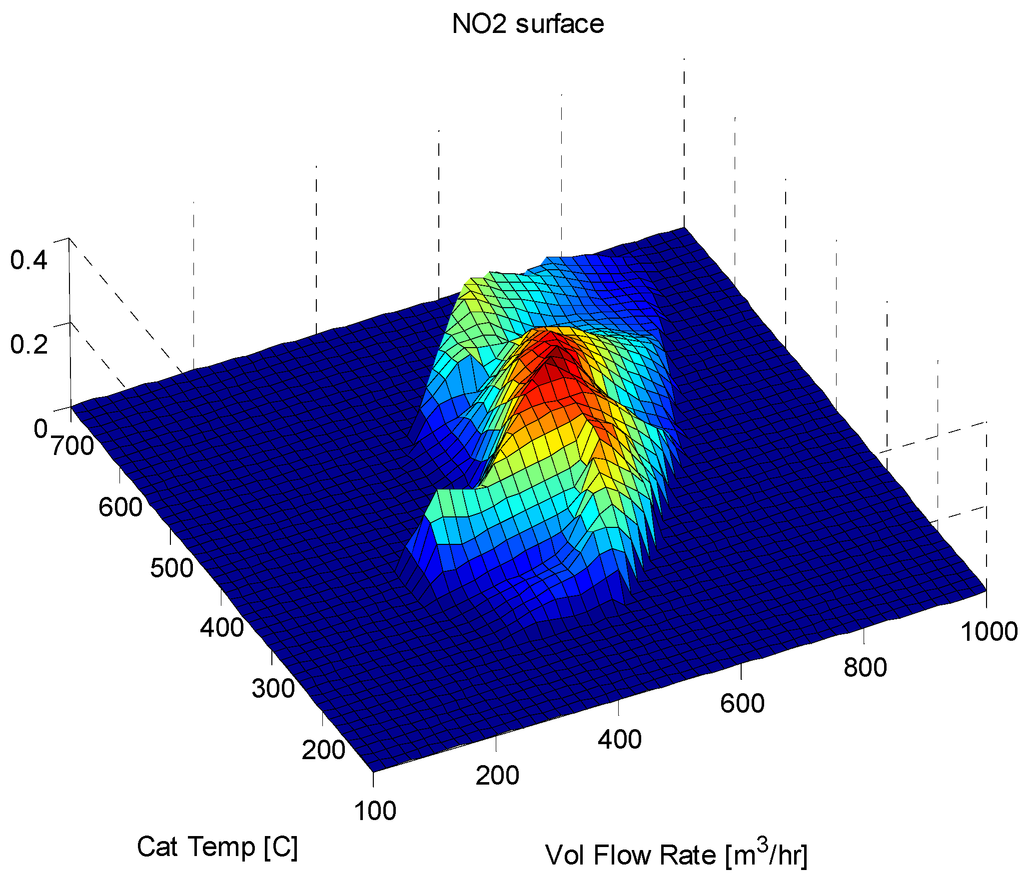
The test to determine the NO2 conversion performance of the oxidation catalyst was performed with the standard exhaust system configuration on the testbed with gas analysis samples taken from upstream of the particulate filter. A full engine map was run which allowed the NOx and NO2 concentrations to be taken over the full range of exhaust temperatures and flows. The data were used to generate a reference surface of the NO2 conversion rate (concentration of NO2/concentration of NOx) with volume flow rate and exhaust gas temperature (Figure 21).
Figure 21.
Surface plot of NO2 conversion rate for the oxidation catalyst.
This surface shows the characteristics of NO2 make with temperature; there is a rapid rise with temperature as the activation energy for the reaction is achieved followed by a gradual reduction as the reaction equilibrium shifts from NO2 towards NO. Similarly, volume flow rate, although not independent of temperature, shows a trend of decreasing NO2 make as volume flow rate increases and therefore residency time decreases. The NO2 make surface was then used to produce the correction curves in the model as per the optimization routine explained earlier.
Color coding differentiates the values. It can be observed that the maximum conversion rate of about 0.4 occurs at mid volume flow rates and slightly higher than mid catalyst temperatures (shown in red).
Surfaces of NO2 make rates were generated for both green and aged components. The effect of ageing was established by comparing these surfaces and calculating the average difference over the whole surface.
7.5. Soot Oxidation by NO2
The first step to calibrate the passive soot regeneration by NO2 was to load the DPFs with soot on a mix of testbed and vehicle cycles. The removeable filters were loaded with 30 g of soot, corresponding to 75% capacity. At soot loadings above this level, the ECU strategy may initiate an active filter regeneration event as soon as a suitable drive cycle is available. The DPFs’ accurate measuring was ensured using the Cambustion Particulate Filter Test System. Soot is hydroscopic but by using this system, where scales are housed within an oven-like setup to drive off any moisture, soot mass can be measured with a resolution of 0.3 g [34].
In some previous studies into the NO2 mechanism, the rate of soot reduction has been determined by measuring the flow rate and the concentration of the products of oxidation, i.e., CO2 and CO [35]. These tests, however, were performed using heaters to raise the temperature of the gas. A similar technique has been used for the investigation of active regeneration. However, the experience showed that because the background levels of CO2 in the exhaust gas are relatively high compared to the difference in CO2 level generated across the filter as the soot burns, this method was at the limit of the capability of the equipment. For the passive regeneration tests where the soot burn rates and therefore CO2 differences are significantly lower, this method would not be sufficiently sensitive. This leaves removing and weighing the filter as the method to determine the soot mass loss as mentioned above.
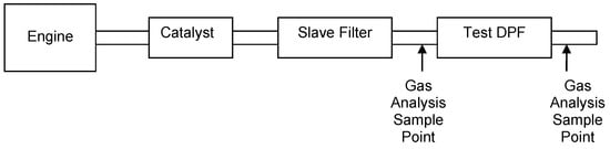
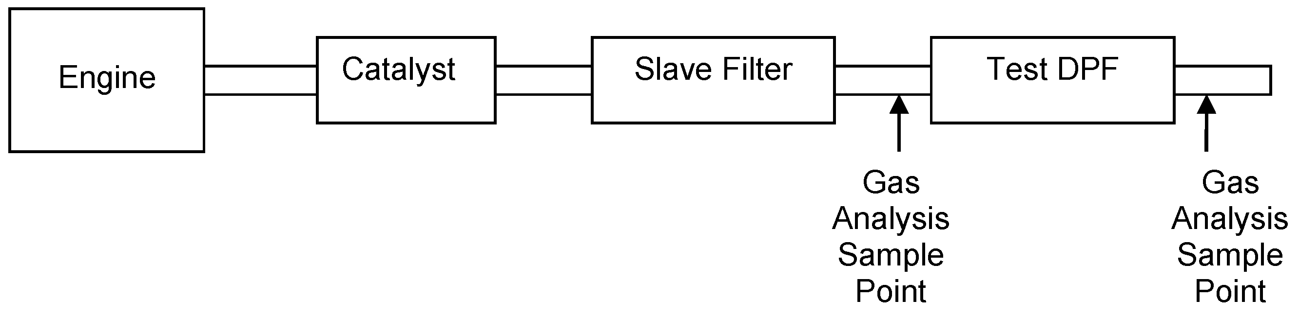
Testing was conducted on testbeds with the configuration shown in Figure 22 to ensure that no soot was allowed to be deposited whilst the test was running. A second uncoated DPF (without the capability of regenerating soot) was fitted between the oxidation catalyst and the test DPF to remove soot particles before they reached the test DPF. As discussed earlier, temperatures for these tests were selected in the range of 250 °C to 450 °C. Engine operating points corresponding to these exhaust temperatures were selected.
Figure 22.
Testbed configuration for mapping the NO2 make in the DPF.
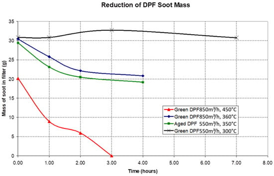
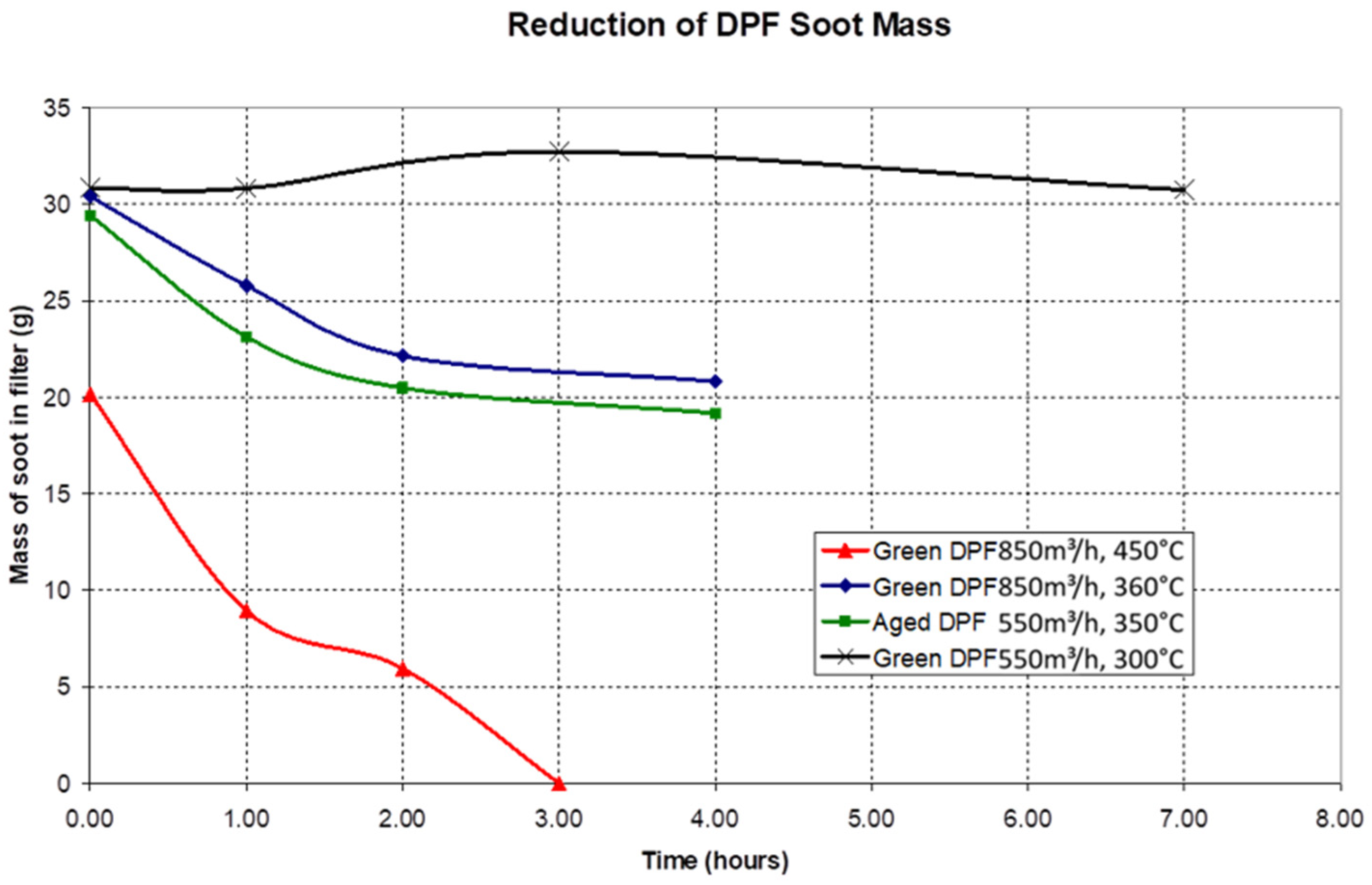
Measurement of soot loss using the oven weighs, at regular intervals, was used to calculate the soot burn rate and also, by implication, the rate at which NO2 was consumed. The plot of soot mass with time (Figure 23) confirms that the rate at which soot is oxidized increases with increasing temperature. However, it also shows that for a temperature of 300 °C at the DPF, no reduction in soot mass was observed. This is a higher minimum temperature than predicted by the literature (reference Figure 10). This variation may have been due to the difference in test setup, especially the temperature measurement, at the soot location. The planned test at 250 °C for our test setup was cancelled as a result.
Figure 23.
Soot mass reduction with time.
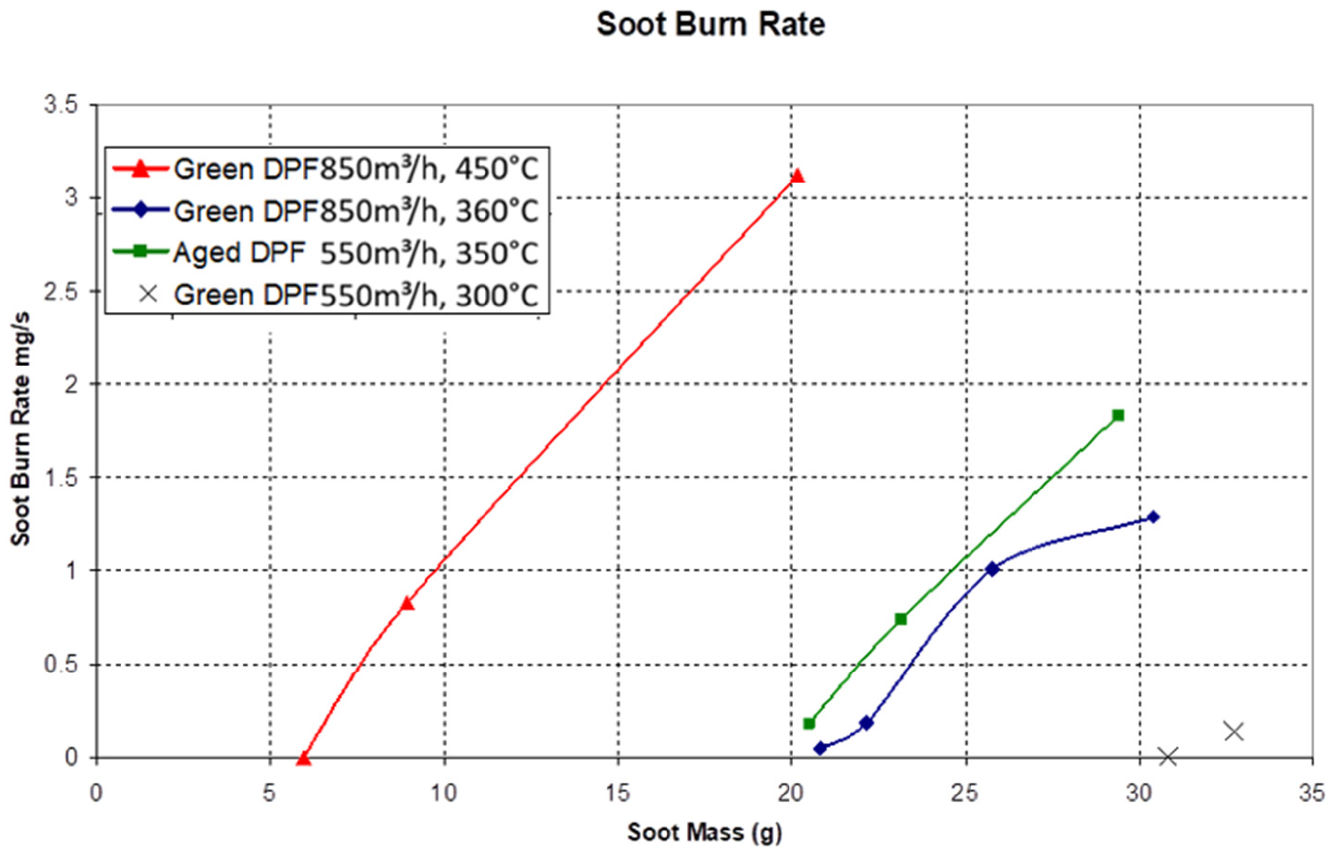
The most interesting results are those taken at 350 °C for the two volume flow rates of 550 m3/h and 850 m3/h. They show that the soot oxidation rate (Figure 24) for the two DPFs, one green and the other aged, were very similar, that the rate at which soot oxidized reduced with time, and that by the time the soot mass had fallen by about 10 g, the rate of soot oxidation had almost dropped to zero.
Figure 24.
Soot oxidation rate.
The similar oxidation rates for the two tests at 350 °C is an important result. It confirms that the rate of soot oxidation is insensitive to the volume flow rate of exhaust gas but is dependent on NO2 flux and the mass of soot in the filter.
With all the parameters for the soot model now calibrated and optimized using the testbed and the vehicle standard drive cycle data, the mode is now ready to be deployed and optimized on the real-world driving conditions. With the provision of running this model offline, the optimisation process is much simpler and removes the need for re-running multiple iterations of test cycles.
8. Real-World Driving Cycle Optimization
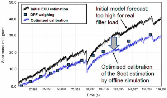
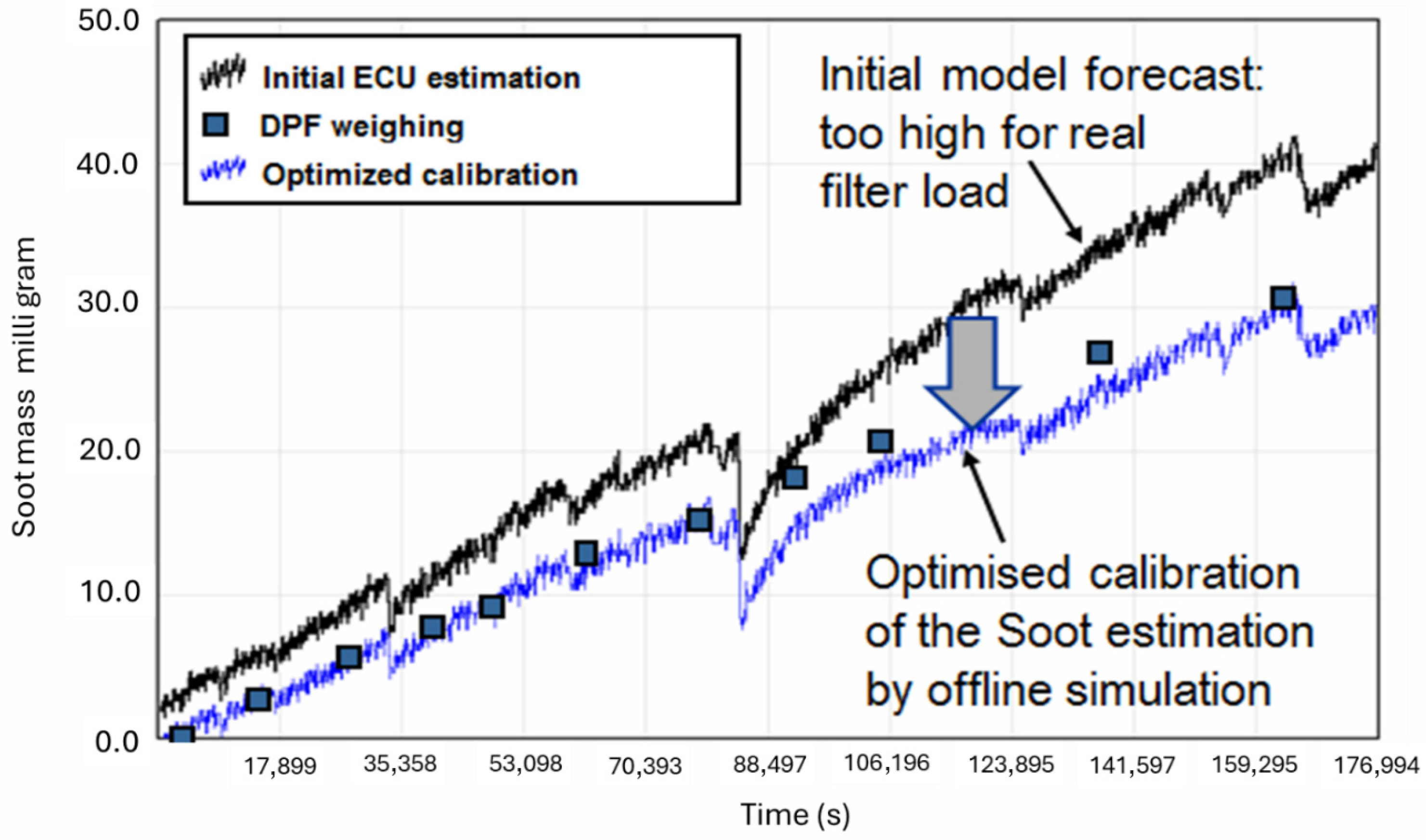
In the next step, the validation of the model on real-world driving conditions was performed whereby the DPF was filled with soot while driving the car on different road conditions. The switching between different modes of powertrain was active during these drives so that the effects of transients, stop–start, cold-start, and extra load during charging, were all captured in these data. The DPF was removed at regular intervals and was weighed on oven scales [34] to give accurate soot weights in the DPF. The model estimation vs. actual weight was plotted and then, using the Simulink model (and the optimisation routines), the maps and parameters were optimized to give an accurate estimate. Figure 25 illustrates one of these loading cycles. This proves the capability of our tool to effectively optimize the soot estimation virtually without the need to run multiple iterations of physical testing.
Figure 25.
Optimization of particulate filter soot load estimation on on-road driving cycles.
One explanation for the initial forecast inaccuracy in soot estimation in real-world road testing is the multitude of operating and environmental conditions not covered in the laboratory testing. Also, the inaccuracies in the measuring equipment, for example, the MSS’s sensitivity to temperature and humidity, make it impossible to accurately calculate the soot emissions. These inaccuracies can only be adjusted when the physical weight of the accumulated soot is available. Also, with the help of the system simulation model, the calibratable parameters can be easily optimized without repeating all the measurements in the laboratory and on the road.
9. Conclusions
For ICE-powered hybrid vehicles, simulation methods and modeling techniques possess significant potential for reducing development costs and time while optimising exhaust aftertreatment system control during transient operations to reduce tailpipe emissions [36]. Transient RDE cycles and hybrid switching can be challenging when estimating correct soot quantities in particulate filters. Optimising DPF regeneration frequency through accurate soot accumulation estimation can offer significant improvements in reducing fuel consumption, CO2, and NOx emissions.
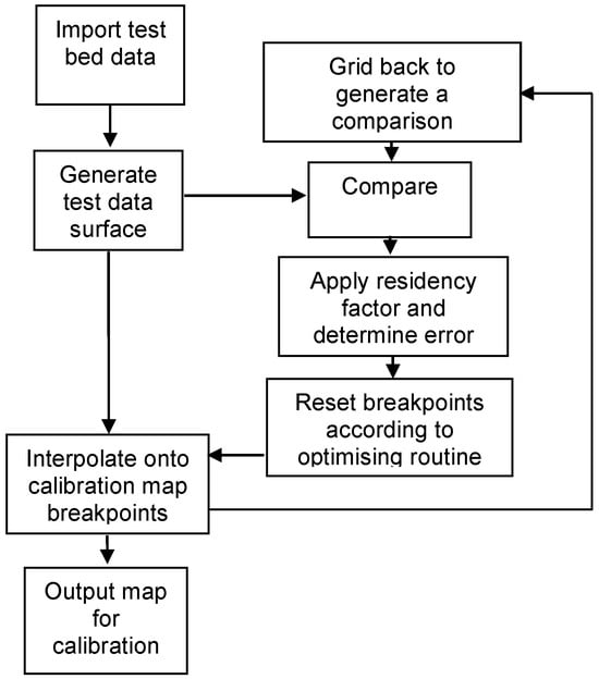
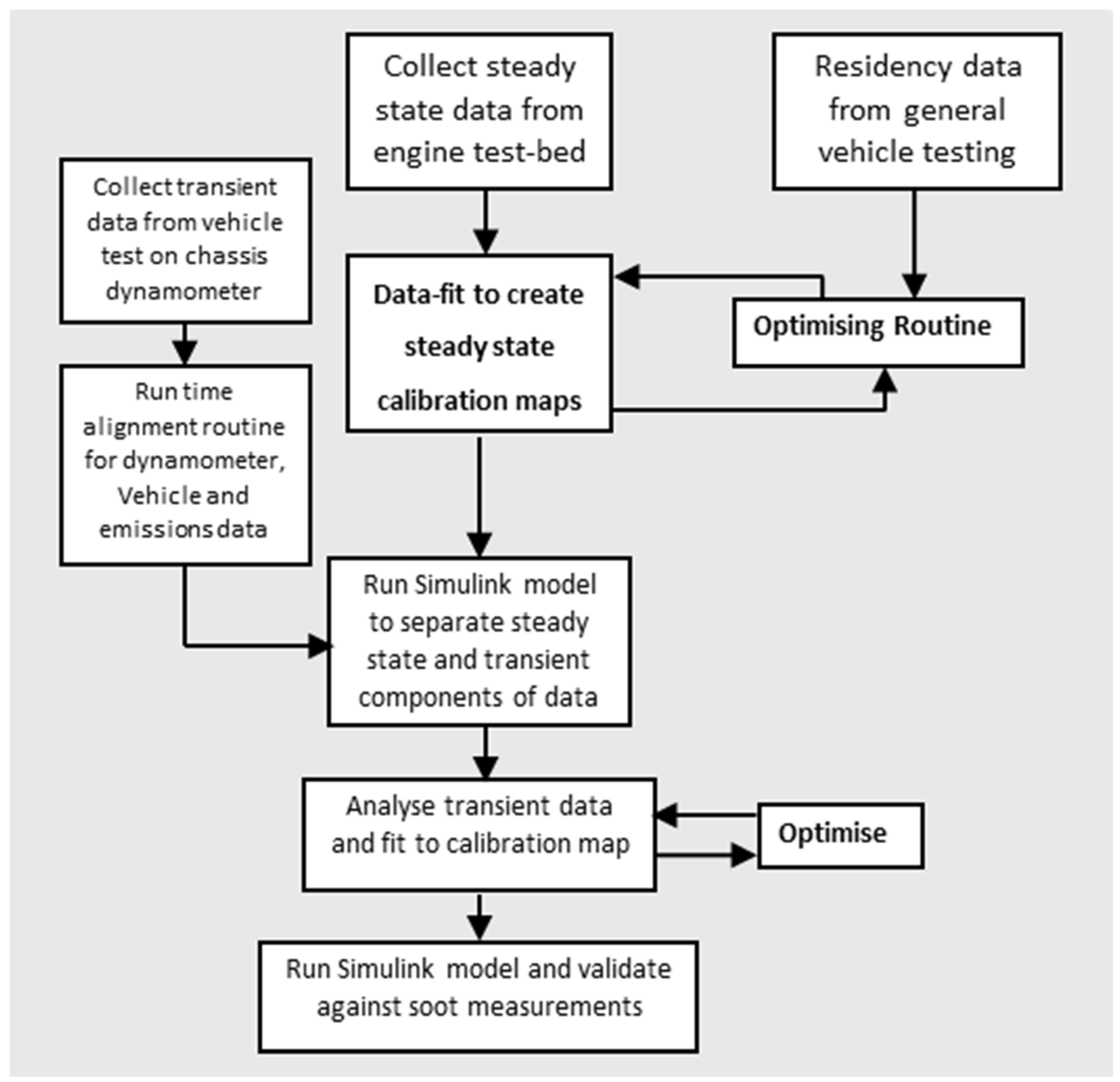
A methodology has been devised, summarized in Figure 26, which is supported by Matlab scripts and Simulink simulations to estimate soot loading in the DPF. This combines a steady-state element with a correction for transient engine operation. Automated optimisation routines were employed to determine the model parameters. This systematic approach enables the optimisation of multiple parameters simultaneously while maintaining the physical relevance of the calibrated values.
Figure 26.
Calibration of the DPF soot load model.
To account for the total soot in the DPF, the rate of soot oxidation by means of the NO2 mechanism is also modeled in three stages: characterising the engine-out NOx emissions; the conversion rate of NO to NO2; and the rate of soot oxidation by NO2. This procedure was carried out with green and aged components to give calibration curves for NO2 make with temperature and volume flow rate, and a correction factor for the ageing of the catalytic coatings over the life of the components.
The innovative soot estimation model developed and optimized in this research demonstrates promising results and adequate accuracy across various real driving cycles. The proposed method improves transient operation accuracy while minimising the requirements for large numbers of iterative experimental tests and analyses of complex chemical reactions required in traditional approaches. This represents a significant advancement in DPF calibration methodology, enabling more efficient development of emission control systems while meeting increasingly stringent regulatory requirements.
Future work should focus on extending this methodology to other aftertreatment components and investigating the integration with advanced predictive control strategies for optimal system-level performance under real-world operating conditions.
Author Contributions
Conceptualization, F.M. and S.P.; methodology, F.M.; software, F.M.; validation, F.M. and S.P.; formal analysis, K.E., F.M. and S.P.; investigation, F.M.; resources, K.E.; data curation, F.M.; writing—original draft preparation, F.M.; writing—review and editing, S.P.; visualization, F.M. and S.P.; supervision, K.E.; project administration, K.E.; funding acquisition, F.M. All authors have read and agreed to the published version of the manuscript.
Funding
This research received no external funding.
Institutional Review Board Statement
Not applicable.
Informed Consent Statement
Not applicable.
Data Availability Statement
The raw data supporting the conclusions of this article will be made available by the authors on request.
Conflicts of Interest
The authors declare no conflict of interest.
Glossary
| AFR | Air–Fuel Ratio |
| ASC | Ammonia Slip Catalyst, additional catalyst used to oxidize residual ammonia (NH3) downstream SCR |
| CO | Carbon monoxide, generated in the combustion chamber where the fuel is in excess locally |
| CO2 | Carbon dioxide, directly related to fuel consumption, to be pushed as low as possible, impacted by the amount and duration of the rich purges |
| DEF | Diesel Exhaust Fluid, aqueous urea solution used to reduce NOx |
| DOC | Diesel oxidation catalyst, catalyst used on diesel vehicles, treating HC and CO after light off |
| DPF | Diesel particulate filter: Since EU5 legislation, used on most diesel vehicles to limit the emission of particulates |
| ECU | Electronic control unit for engine and aftertreatment systems control |
| EGR | Exhaust gas recirculation, technology looping exhaust gases back with fresh air for emission control |
| EU5–EU6–EU6c–EU6d | Emission standards in Europe, respectively, introduced in 2009–2014–2017–2020 |
| FIO | Fuel-in-oil. The phenomenon whereby some of the fuel is injected late during the combustion cycle, to increase exhaust temperature for DPF regeneration; mixes up with the engine oil and causes dilution |
| FTP75 | (Federal Test Procedure), driving cycle (among others) for North American emission certification |
| H2 | Dihydrogen. H2 is a by-product of the combustion in rich, from steam reforming reactions, and also within the catalyst. H2 is a very active contributor to the reduction reactions, but is present in smaller quantities than CO. It also has a significant impact on the generation of NH3 in the catalyst |
| HC | Hydrocarbon, non-burnt hydrocarbons, like the CO, product of the poor mixture of the fuel and the fresh air. The HCs can be different chemical compositions (methane, hexane, decane, etc.). HCs are also reductants for the purges, but are much less active and prompt to react than the CO or H2, and have adverse effect on the LNT on the purge phases |
| LNT | Lean NOx trap: Catalyst used for storage and reduction in NOx (NO and NO2) by chemically capturing the NOx and converting them by changing the stoichiometry of the exhaust gases. It also has the functionality of an oxidation catalyst, treating HC and CO |
| MSS | Micro soot sensor, device for continuous soot measurement |
| NOx | Nitrous oxides, composed by NO and NO2, regulated pollutant critical for current and future emission legislation compliance |
| NEDC | (New European driving cycle): Driving cycle used in Europe for emission certification and fuel consumption evaluation |
| RDE | Real Driving Emissions (introduced EU 2017), mandatory test procedure conducted on-road in real-world conditions with PEMS units fitted to the vehicle tailpipe |
| SCR | This is a means of converting nitrogen oxides with the aid of a catalyst into N2, and water, a gaseous reductant, typically urea, is added to a stream of flue or exhaust gas and is adsorbed onto a catalyst. By extension, this also refers to the catalyst itself |
| SCRF | Diesel particulate filter, with an SCR coating to treat particulates and NOx at the same time |
Appendix A. Physical Equations for a DPF Soot Estimation Model on a Passenger Car
Below is a physics-based (control-oriented) set of equations commonly used to estimate soot mass in a DPF on a passenger car. This is the type of model used in production ECUs [37].
Appendix A.1. Engine-Out Soot Formation (Input to DPF)
The DPF soot balance starts with engine-out particulate mass flow (A1):
where = exhaust mass flow [kg/s], = engine-out soot concentration [kg/kg_exh].
Control-Oriented Soot Map
In ECUs, the soot concentration is map-based (A2):
where in addition to Section 6.2. Model Formulation parameters, = relative exhaust air to fuel ratio [-], = fuel rail pressure [bar]. However, a typical simplified regression form can be expressed in (A3):
where are constants which need to be determined.
Appendix A.2. Soot Deposition in the DPF (Filtration)
Filtration efficiency can be expressed in (A4):
where [kg−1] is the filtration build-up constant, meaning the rate at which filtration efficiency increases with soot cake. Typically, , the fraction of incoming soot trapped by the DPF starts ~70–90%, and approaches 99% as cake builds up.
Soot mass accumulation is then defined in (A5):
Appendix A.3. Soot Oxidation (Regeneration)
Total soot oxidation consists of passive (NO2) and active (O2) terms.
Appendix A.3.1. Passive Regeneration (NO2-Assisted)
NO2 regeneration is defined in (A6):
which occurs in the temperature in the range 250–400 °C. is the chemical reaction rate constant for [kg−1m−2Pa−1], [m2] is the effective soot reaction surface area, [Pa] is the partial pressure of in the exhaust gas, typically 1–50 Pa, [Jmol−1] is the activation energy for . [K] is the DPF brick temperature and [Jmol−1K−1] is the Universal Gas Constant.
Appendix A.3.2. Active Regeneration (O2 Oxidation)
O2 regeneration is defined in (A7):
which occurs at temperatures >550–650 °C. is the chemical reaction rate constant for [kg−1m−2Pa−1], [Pa] is the partial pressure of in the exhaust gas, typically 5–15 kPa, [Jmol−1] is the activation energy for .
Appendix A.3.3. Total Oxidation Rate
The total soot oxidation rate (passive + active) is calculated in (A8):
Appendix A.4. DPF Soot Mass Balance (Core Estimation Equation)
Applying mass balance, the central physical Equation (A9) is derived:
Appendix A.5. DPF Pressure Drop Model (Used for Correction)
The pressure drop across the filter [mbar] is used as a representation of the soot loading. The measured pressure drop is compared to the estimated one and used to correct the model-based soot estimator in (A10):
For a clean DPF, the pressure drop is in the range 5–20 mbar.
The total pressure drop can be modelled as the sum of the wall flow term and the soot caking part in (A11) and (A12):
where [Pas] is the exhaust dynamic viscosity, [m] is the length of the PDF channel wall, [ms−1] is the superficial velocity through the wall, [m2] is the porosity/permeability of ceramic wall. [Pakg−1(kgs−1)−n] is the soot cake pressure coefficient, is a tuning factor 1.0–1.2.
Appendix A.6. Typical Passenger Car Values (Order of Magnitude)
| Parameter | Typical Value |
| Max soot load | 20–30 g |
| Passive regen temp | 250–400 °C |
| Active regen temp | 600–650 °C |
| Δp full DPF | 80–120 mbar |
| Filtration efficiency | 90–99% |
| Soot oxidation heat | ~30 MJ/kg |
References
- Johnson, T. Diesel Emissions in Review. SAE Int. J. Engines 2011, 4, 143–157. [Google Scholar] [CrossRef] [Scilit]
- Kuwahara, T.; Nishii, S.; Kuroki, T.; Okubo, M. Complete regeneration characteristics of diesel particulate filter using ozone injection. Appl. Energy 2013, 111, 652–656. [Google Scholar] [CrossRef] [Scilit]
- Liu, H.W.; Yao, G.T.; Jiang, D.H.; Zi, X.Y.; Guo, Z.R. Design and Experimental Research on Evaporation-Type DPF Regenerative Burner. Appl. Mech. Mater. 2012, 229, 1025–1029. [Google Scholar] [CrossRef] [Scilit]
- Franco, V.; Posada, F.; German, J.; Mock, P. Real-World Exhaust Emissions from Modern Diesel Cars. 1 October 2014, The International Council on Clean Transportation. Available online: https://theicct.org/wp-content/uploads/2021/06/ICCT_PEMS-study_diesel-cars_20141013_0.pdf (accessed on 11 December 2025).
- Schejbal, M.; Marek, M.; Kubíček, M.; Kočí, P. Modelling of diesel filters for particulates removal. Chem. Eng. J. 2009, 154, 219–230. [Google Scholar] [CrossRef] [Scilit]
- Depcik, C.; Assanis, D. Simulating Area Conservation and the Gas-Wall Interface for One-Dimensional Based Diesel Particulate Filter Models. J. Eng. Gas Turbines Power 2008, 130, 062807. [Google Scholar] [CrossRef] [Scilit]
- Valeria, D.S.; Almerinda, D.B. Modeling and simulation of soot combustion dynamics in a catalytic diesel particulate filter. Chem. Eng. Sci. 2015, 137, 69–78. [Google Scholar] [CrossRef] [Scilit]
- Stamatelos, A.M. A review of the effect of particulate traps on the efficiency of vehicle diesel engines. Energy Convers. Manag. 1997, 38, 83–99. [Google Scholar] [CrossRef] [Scilit]
- Ogyu, K.; Yamakawa, T.; Ishii, Y.; Minoura, D.; Nagatsu, Y.; Kasuga, T.; Ohno, K. Soot loading estimation accuracy improvement by filtration layer forming on DPF and new algorithm of pressure loss measurement. SAE Tech. Pap. 2013, 2, 421–422. [Google Scholar]
- Roberts, J.; Evans, C.; Turner, L. Strategies To Diminish the Emissions of Particles and Secondary Aerosol Formation from Diesel Engines. Environ. Sci. Technol. 2019, 53, 10408–10416. [Google Scholar] [CrossRef] [Scilit]
- Rose, D.; Boger, T. Different Approaches to Soot Estimation as Key Requirement for DPF Applications 2009-01-1262. In Proceedings of the SAE World Congress & Exhibition, Detroit, MI, USA, 20 April 2009. [Google Scholar]
- Available online: https://www.sae.org/publications/technical-papers/content/2009-01-1262/ (accessed on 11 December 2025).
- Boretto, G.; Imarisio, R.; Rellecati, P.; Barucchi, E.; Sanguedolce, A. Serial Application of a Catalyzed Particulate Filter on Common Rail DI Diesel Engines for Passenger Cars; F2004V068; FISITA World Automotive Congress: Barcelona, Spain, 2004. [Google Scholar]
- Phillips, G.; Moore, K.; Wright, D. European Regulatory Framework and Particulate Matter Emissions of Gasoline Light-Duty Vehicles: A Review. Catalysts 2019, 9, 586. [Google Scholar] [CrossRef] [Scilit]
- Thompson, K.; Anderson, R.; Wilson, S. The Process of Diesel Particulate Filter Regeneration under Real Driving Conditions. Earth Environ. Sci. 2019, 214, 012114. [Google Scholar]
- Allansson, R. Optimising the Low Temperature Performance and Regeneration Efficiency of the Continuously Regenerating Diesel Particulate Filter System. SAE 2002-01-0428. SAE Tech. Pap. 2002. [Google Scholar] [CrossRef] [Scilit]
- Fiebig, M.; Wiartalla, A.; Holderbaum, B.; Kiesow, S. Particulate emissions from diesel engines: Correlation between engine technology and emissions. J. Occup. Med. Toxicol. 2014, 9, 6. [Google Scholar] [CrossRef] [Scilit]
- Pischinger S: Verbrennungskraftmaschinen, 26th ed.; Lecture Notes; RWTH-Aachen University: Aachen, Germany, 2007; Volume 2.
- Knörr, W.; Kutzner, F.; Lambrecht, U.; Schacht, A. Daten- und Rechenmodell: Energieverbrauch und Schadstoffemissionen. Heidelberg GmbH: TREMOD; Endbericht ifeu—Institut für Energie und Umweltforschung: Wilckensstraße, Heidelberg, 2010. [Google Scholar]
- IFEU. 6. Immissionsschutzbericht; Institute for Energy and Environmental Research: Wilckensstraße, Heidelberg, 1996. [Google Scholar]
- Martinez, A.; Rodriguez, B.; Garcia, C. Diesel Particle Filter Requirements for Euro 7 Technology Continuously Regenerating Heavy-Duty Applications. Vehicles 2023, 5, 89. [Google Scholar] [CrossRef] [Scilit]
- Ohyama, N.; Nakanishi, T.; Daido, S. New Concept Catalyzed DPF for Estimating Soot Loadings from Pressure Drop 2008-01-0620. In Proceedings of the SAE World Congress & Exhibition, Detroit, MI, USA, 14 April 2008. [Google Scholar]
- Available online: https://www.sae.org/publications/technical-papers/content/2008-01-0620/ (accessed on 11 December 2025).
- Gai, Y.; Yao, P.; Li, S.; Zhang, H.; Wu, Y.; Jiao, Y.; Chen, Y.; Wang, J. Real biofuel and fossil-fuel soot combustion activities in active and passive regeneration of diesel/gasoline particulate filters under different O2/NOx concentrations. Environ. Sci. Pollut. Res. 2024, 31, 45718–45733. [Google Scholar] [CrossRef] [Scilit]
- Twigg, M.V.; Phillips, P.R. Cleaning the Air We Breathe—Controlling Diesel Particulate Emissions from Passenger Cars. Platin. Met. Rev. 2009, 53, 27–34. [Google Scholar] [CrossRef] [Scilit]
- Johnson, T.V. Diesel Emission Control Technology-2003 in Review. SAE Tech. Paper No. 2004-01-0070. SAE Tech. Pap. 2004. [Google Scholar] [CrossRef] [Scilit]
- Kim, J.H.; Kim, M.Y.; Kim, H.G. NO2-Assisted Soot Regeneration Behavior in a Diesel Particulate Filter with Heavy-Duty Diesel Exhaust Gases. Numer. Heat Transf. Part A 2010, 58, 725–739. [Google Scholar] [CrossRef] [Scilit]
- Jeguirim, M.; Tschamber, V.; Ehrburger, P. Catalytic effect of platinum on the kinetics of carbon oxidation by NO2 and O2. Appl. Catal. B Environ. 2007, 76, 235–240. [Google Scholar] [CrossRef] [Scilit]
- Commission Regulation (EU). Amending Regulation (EC) No 692/2008; 2016/646 of 20 April 2016; Official Journal of the European Union: Luxembourg; pp. L109/1–L109/98.
- Giakoumis, E.G.; Zachiotis, A.T. Comparative Evaluation of Eight Legislated Driving Schedules in Terms of Cycle Metrics and Emissions from a Diesel-Powered Turbocharged Van. Transp. Res. Part D Transp. Environ. 2018, 58, 139–154. [Google Scholar] [CrossRef] [Scilit]
- International Council on Clean Transportation (ICCT). Real-Driving Emissions Test Procedure for Exhaust Gas Emissions of Road Vehicles. 2017. Available online: https://theicct.org (accessed on 11 December 2025).
- Wang, L.; Zhou, M.; Zhang, P. Estimation of the Diesel Particulate Filter Soot Load Based on an Equivalent Circuit Model. Energies 2018, 11, 472. [Google Scholar] [CrossRef] [Scilit]
- Ohno, K.; Shimato, K.; Toaka, N.; Hong, S.; Ninomiya, T.; Komori, T.; Salvat, O. Characterization of SiC-DPF for Passenger Car. SAE Technical Paper 2000-01-0185. SAE Tech. Pap. 2000. [Google Scholar] [CrossRef] [Scilit]
- Hands, T.; Twigg, M.V.; Gallinger, M. A New Instrument for Diesel Particulate Filter Functional Tests in Development and Quality Control Applications. SAE Paper 2010-01-0809. SAE Tech. Pap. 2010. [Google Scholar] [CrossRef] [Scilit]
- Jay, H.; Lee, H.-S.; Song, S.; Chun, K.M. Experimental investigation of soot oxidation characteristic with NO2 and O2 using a flow reactor simulating DPF. SAE 2007-01-1270. SAE Tech. Pap. 2007. [Google Scholar] [CrossRef] [Scilit]
- Nelson, V.; Foster, W.; Price, J. Effects analysis on soot oxidation performance in the diesel particulate filter based on synergetic passive-active composite regeneration methods. Chem. Eng. Sci. 2022, 262, 118013. [Google Scholar] [CrossRef] [Scilit]
- Cozzolini, A.; Mulone, V.; Abeyratne, P.; Littera, D.; Gautam, M. Advanced Modeling of Diesel Particulate Filters to Predict Soot Accumulation and Pressure Drop. 2011-24-0187. SAE Tech. Pap. 2011. [Google Scholar] [CrossRef] [Scilit]
Disclaimer/Publisher’s Note: The statements, opinions and data contained in all publications are solely those of the individual author(s) and contributor(s) and not of MDPI and/or the editor(s). MDPI and/or the editor(s) disclaim responsibility for any injury to people or property resulting from any ideas, methods, instructions or products referred to in the content. |
© 2026 by the authors. Licensee MDPI, Basel, Switzerland. This article is an open access article distributed under the terms and conditions of the Creative Commons Attribution (CC BY) license.