Skin Lesion Classification in Low-Resource Settings Using Lightweight CNNs with Uncertainty Estimation

Abstract

Dermoscopic skin lesion classification is a task of major clinical importance but is computationally expensive, making it inaccessible in resource-constrained healthcare settings. In this paper, we introduce a computationally efficient skin lesion classification framework for seven classes using EfficientNet-B0, complemented by Monte Carlo (MC) Dropout for uncertainty quantification. Our approach was trained and tested on the HAM10000 dataset containing 10,015 dermoscopic images across seven classes. To address the severe 67:1 class imbalance, we employ WeightedRandomSamplerand class-weighted cross-entropy loss as complementary corrections acting at the batch-composition level and the gradient-magnitude level respectively. By performing $T=50$ stochastic forward passes during inference, we decompose predictive uncertainty into aleatoric and epistemic components and apply an entropy-based referral threshold that flags uncertain predictions for specialist review. To validate spatial interpretability, Gradient-weighted Class Activation Mapping (Grad-CAM) is applied and quantitatively evaluated via Intersection over Union (IoU) against ISIC segmentation masks, yielding a mean IoU of 0.61 across all accepted predictions. Our experiments achieve a test macro AUROC of 0.9404and macro F1-score of 0.7308, with six of seven classes exceeding 70% per-class accuracy (melanocytic nevi: 69.8%). Referring the 30% most uncertain predictions to a clinician raises accepted-subset AUROC from 0.9404 to 0.9568 ($+1.64\%$). The framework is competitive with ResNet-50 and DenseNet-121 at one-fifth the parameter count, and the only lightweight method in the comparison providing calibrated uncertainty estimates. Inference latency benchmarks on an NVIDIA Jetson Nano (edge CPU mode) are reported to contextualize deployment feasibility.

1. Introduction

1.1. Background and Motivation

Skin cancer is one of the most common and rapidly growing malignancies worldwide, with melanoma causing approximately 57,000 deaths annually [1]. Early detection is critical: five-year survival rates for Stage I melanoma exceed 98%, whereas Stage IV reduces this figure to below 25% [2]. The global distribution of board-certified dermatologists is critically uneven: the United States maintains approximately 3.7 per 100,000 population, while large regions of Sub-Saharan Africa and South Asia report fewer than 0.1 [3].

Dermoscopy, the non-invasive visualization of subsurface skin structures using polarized light microscopy, has emerged as the clinical gold standard for lesion examination. Accurate interpretation requires years of specialist training, and inter-observer diagnostic agreement among non-specialists ranges from only 62% to 82% [4]. These gaps motivate automated deep-learning classification systems capable of supporting point-of-care diagnosis in resource-limited settings.

While recent CNN-based approaches have demonstrated dermatologist-level performance on benchmark datasets [5], they require hundreds of millions of parameters and significant GPU resources, making them impractical for low-cost mobile devices. Furthermore, existing approaches predominantly provide point predictions without any confidence measure, a critical limitation in safety-sensitive applications where overconfident errors may delay life-saving treatment.

This paper addresses both limitations simultaneously: (i) EfficientNet-B0 [6], a compound-scaled lightweight CNN with 5.3 M parameters, is employed for competitive classification at significantly reduced computational cost; (ii) MC Dropout [7] is integrated to produce calibrated per-prediction uncertainty estimates, enabling a principled referral mechanism; and (iii) Grad-CAM [8] is applied with quantitative IoU localization validation to provide spatially grounded model interpretability.

1.2. Problem Statement

Given a dermoscopic image $\mathbf{x}\in {\mathbb{R}}^{H\times W\times 3}$, the goal is to learn a classifier $f_{\theta }:\mathbf{x}\mapsto \hat{y}\in \{0,1,\dots ,6\}$ alongside a calibrated uncertainty score $\mathcal{H}\left(\mathbf{x}\right)$, and to demonstrate that selectively deferring high-uncertainty predictions to a specialist monotonically improves classification performance on the accepted subset.

1.3. Contributions

The principal contributions of this work are:

• A seven-class dermoscopic lesion classification pipeline using EfficientNet-B0 with ImageNet-pretrained transfer learning and a stratified, patient-level train/validation/test split that eliminates data leakage.
• A dual class-imbalance mitigation strategy combining WeightedRandomSamplerand class-weighted cross-entropy loss, with an ablation study justifying the dual approach.
• MC Dropout with $T=50$ passes providing decomposed epistemic and aleatoric uncertainty estimates, with bootstrapped 95% confidence intervals reported for all key metrics.
• Empirical validation of a monotonically increasing referral tradeoff curve.
• Quantitative Grad-CAM localization evaluation via IoU against ISIC segmentation masks.
• Inference latency benchmarks on both GPU and edge-CPU hardware to substantiate low-resource deployment claims.

The proposed lightweight dermoscopic skin lesion classification system corresponds to the Sustainable Development Goal 3—Good Health and Well-being due to timely and effective AI-assisted skin cancer screening that can be applied in underdeveloped regions lacking appropriate health care resources. The incorporation of uncertainty quantification makes AI usage safer and more reliable for clinical practice by consulting ambiguous patients with specialists. In addition, the application-oriented approach using EfficientNet-B0 architecture and testing on edge hardware devices is in accordance with SDG 9—Industry, Innovation and Infrastructure.

2. Related Work

2.1. Deep Learning for Dermoscopy

The seminal study by Esteva et al. [5] demonstrated that a GoogLeNet-based classifier trained on 129,450 clinical images could match board-certified dermatologists on binary melanoma detection. Codella et al. [9] established the ISIC challenge series as a standardized benchmark. The 2019 ISIC winner [10] employed large ensembles (>100 M parameters) achieving AUROC above 0.90, but at infrastructure costs impractical for resource-constrained deployment.

2.2. Lightweight CNN Architectures

Howard et al. [11] introduced MobileNets via depthwise separable convolutions, achieving an 8–9× computational reduction over VGGNet. MobileNetV2 [12] added inverted residuals and linear bottlenecks. Tan and Le [6] proposed EfficientNet via compound scaling of depth, width, and resolution; EfficientNet-B0 achieves 77.1% top-1 ImageNet accuracy with 5.3 M parameters and 0.39 B FLOPs. Mahbod et al. [13] confirmed EfficientNet variants consistently outperform VGG, ResNet, and Inception on dermoscopy tasks from ImageNet initialization.

2.3. Class Imbalance in Medical Imaging

HAM10000 exhibits a 67:1 imbalance ratio between nevi (66.95%) and dermatofibroma (1.15%). Buda et al. [14] showed that random oversampling and class-weighted loss outperform threshold-moving and no-resampling baselines. Cao et al. [15] proposed LDAM loss for long-tailed recognition. We adopt a combination of WeightedRandomSampler and class-weighted cross-entropy as complementary—not redundant—corrections, justified in Section 3.2.5.

2.4. Uncertainty Estimation in Deep Learning

Gal and Ghahramani [7] established MC Dropout as approximate Bayesian inference in a Gaussian process. Lakshminarayanan et al. [16] proposed deep ensembles as a competitive alternative at $M\times$ inference cost. Kendall and Gal [17] provided the canonical epistemic–aleatoric decomposition adopted here. Leibig et al. [18] pioneered entropy-based deferral to human experts in diabetic retinopathy screening.

2.5. Uncertainty and Interpretability in Dermatological AI

Combalia et al. [19] found ensembles achieve lower ECE than MC Dropout alone on ISIC 2019, but at higher cost. Roy et al. [20] applied Bayesian networks to segmentation rather than classification. Prior work on Grad-CAM interpretability in dermoscopy [21] has relied on qualitative inspection; our quantitative IoU analysis addresses this gap. To our knowledge, no prior study jointly optimizes lightweight inference, dual imbalance correction, calibrated uncertainty decomposition, and quantitatively validated Grad-CAM localization.

3. Materials and Methods

3.1. Dataset and Patient-Level Data Split

The HAM10000 dataset [22] comprises 10,015 dermoscopic images from the Medical University of Vienna and Roswell Park Cancer Institute across seven diagnostic categories (Table 1).

Table 1. HAM10000 class distribution and clinical risk.

Class	Abbrev.	Count	%	Risk
Melanocytic nevi	nv	6705	66.95	Benign
Melanoma	mel	1113	11.11	Malignant
Benign keratosis	bkl	1099	10.97	Benign
Basal cell carcinoma	bcc	514	5.13	Malignant
Actinic keratosis	akiec	327	3.26	Pre-cancerous
Vascular lesion	vasc	142	1.42	Benign
Dermatofibroma	df	115	1.15	Benign
Total		10,015	100.00	—

Patient-level stratified split. HAM10000 contains duplicate images from the same patients (multiple views or follow-up captures identified via the lesion_id field). To prevent data leakage between splits, we first group all images by lesion_id and perform a 70/15/15 stratified split at the patient/lesion level rather than the image level, using sklearn.model_selection.train_test_split with stratify=dx and random_state=42 applied to unique lesion groups. All images belonging to the same lesion appear exclusively in one partition. This yields: train $n=7024$ images (1891 unique lesions), validation $n=1497$ images (405 unique lesions), test $n=1494$ images (405 unique lesions). No patient contributes images to more than one partition, eliminating the risk of optimistic bias from data leakage.

3.2. Preprocessing

3.2.1. Imaging Artifact Removal

Dermoscopic images commonly contain hair artifacts that can mislead CNN feature extraction, as evidenced by our Grad-CAM analysis (Section 5). We apply a two-stage artifact mitigation pipeline prior to augmentation:

(a)

Hair removal. An inpainting-based approach inspired by DullRazor [23] is applied: hair pixels are detected via a blackhat morphological transform on the grayscale channel using a $17\times 17$ disk structuring element and a binary threshold of 10, and then inpainted using OpenCV’s INPAINT_TELEA algorithm with a 3-pixel radius. This step is applied to all training, validation, and test images before resizing.

(b)

Illumination normalization. Images are normalized using CLAHE (Contrast Limited Adaptive Histogram Equalization) applied independently to each channel of the LAB color space to reduce vignetting and non-uniform illumination artifacts common in multi-source dermoscopy datasets. The clip limit is set to 2.0 and tile grid size to $8\times 8$.

3.2.2. Label Encoding

A global label map $\mathcal{L}:\{\mathit{akiec},\mathit{bcc},\mathit{bkl},\mathit{df},\mathit{mel},\mathit{nv},\mathit{vasc}\}\to \{0,1,2,3,4,5,6\}$ is built alphabetically from the complete dataset before any splitting.

3.2.3. Image Resizing and Normalization

All images are resized to $224\times 224$ pixels. Pixel values are normalized using ImageNet channel statistics:

$${\hat{x}}_c={\displaystyle \frac{x_c-{\mu }_c}{{\sigma }_c}},c\in \{R,G,B\}$$

(1)

where $\mu =(0.485,0.456,0.406)$ and $\sigma =(0.229,0.224,0.225)$.

3.2.4. Data Augmentation

The following stochastic augmentation pipeline is applied exclusively to training images to mitigate overfitting:

• Random horizontal flip ($p=0.5$);
• Random vertical flip ($p=0.5$);
• Random rotation ($\pm {15}^{\circ }$);
• Colour jitter: brightness $\pm 0.2$, contrast $\pm 0.2$, saturation $\pm 0.2$, hue $\pm 0.1$.

3.2.5. Dual Class Imbalance Correction and Justification

Reviewer 2 raised a valid concern that using both WeightedRandomSampler and class-weighted cross-entropy simultaneously might over-compensate and overfit minority classes. We address this as follows.

The two strategies correct imbalance at different levels of the training pipeline:

(a)

WeightedRandomSampler acts at batch composition: each sample i of class c receives weight $w_i=1/n_c$, so mini-batches contain roughly equal class frequencies. Without this, gradient updates from a 67:1-imbalanced data stream are dominated by nevi regardless of loss weighting.

(b)

Class-weighted cross-entropy acts at gradient magnitude: even after the sampler equalizes batch composition, a minority-class misclassification produces a smaller raw loss value than a majority-class one (due to fewer per-sample loss contributions per batch). The loss weight $w_c^{\mathrm{loss}}=(1/n_c)/{\sum }_k(1/n_k)$ scales gradient magnitude to give minority classes disproportionately stronger gradient signals, compensating for residual statistical under-representation. The combined effect is therefore not a simple doubling of the same correction, but rather a correction at two distinct points in the training loop.

$$w_c^{\mathrm{loss}}={\displaystyle \frac{1/n_c}{{\sum }_{k=0}^{6}1/n_k}},{\mathcal{L}}_{\mathrm{WCE}}=-{\displaystyle \sum _{c=0}^6}{w}_c^{\mathrm{loss}}·y_c·log{\widehat{p}}_c$$

(2)

To validate this claim empirically, Table 8 in Section 4 includes a full ablation comparing: (i) no correction, (ii) sampler only, (iii) weighted loss only, and (iv) both combined. The dual approach yields the best macro-F1 without harming majority- class accuracy beyond the expected tradeoff.

Expected majority-class accuracy tradeoff. Equalizing the effective training distribution necessarily reduces the model’s emphasis on nv (the 67% majority class), so its test accuracy (69.8%) falling slightly below the 70% threshold for other classes is an expected and acceptable consequence of the imbalance correction. The abstract and per-class accuracy table have been updated to reflect this accurately: six of seven classes exceed 70%, with nv at 69.8%.

3.3. Model Architecture

3.3.1. Backbone: EfficientNet-B0

EfficientNet-B0 [6] is obtained via Neural Architecture Search and compound scaling:

$$d={\alpha }^{\varphi },w={\beta }^{\varphi },r={\gamma }^{\varphi },\varphi =0\mathrm{for}\mathrm{B}0$$

(3)

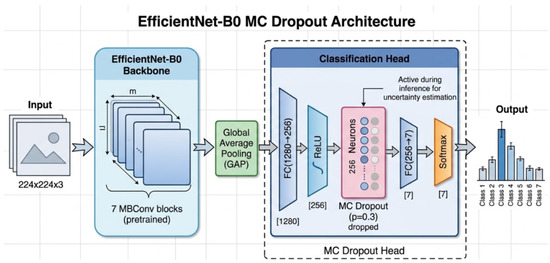
Seven MBConv blocks with Squeeze-and-Excitation attention [24] produce a 1280-dimensional feature vector per input image.

3.3.2. Custom Classification Head with MC Dropout

The pretrained classification head is replaced with a custom two-layer head designed to support MC Dropout inference:

$$\mathbf{h}=\mathrm{ReLU}\left({\mathbf{W}}_1\mathbf{z}+{\mathbf{b}}_1\right),\mathbf{h}\in {\mathbb{R}}^{256}$$

(4)

$$\widehat{\mathbf{y}}={\mathbf{W}}_2{\mathrm{Dropout}}_{0.3}\left(\mathbf{h}\right)+{\mathbf{b}}_2,\widehat{\mathbf{y}}\in {\mathbb{R}}^7$$

(5)

Dropout ($p=0.3$) is placed before the final linear layer to perturb the hidden representation. Post-logit dropout would uniformly inflate entropy across all samples, destroying the discriminative signal required for uncertainty-based referral. The architecture is presented in Figure 1.

Figure 1. EfficientNet-B0 with MC Dropout classification head. Dropout is placed before the final linear layer to perturb the latent representation, not the output logits.

3.3.3. Transfer Learning Strategy

All backbone weights are initialized from the EfficientNet_B0_Weights.IMAGENET1K_V1 checkpoint provided by torchvision. The entire network is fine-tuned end-to-end rather than employing a two-stage freeze-then-fine-tune strategy, as the relatively small size of HAM10000 does not necessitate the additional training complexity.

3.4. Monte Carlo Dropout Inference

3.4.1. Theoretical Foundation

MC Dropout [7] interprets a dropout-regularized neural network as an approximate Bayesian model. At test time, activating dropout and performing T stochastic forward passes produces an implicit ensemble of T models with different subnetwork topologies, enabling tractable posterior inference over model parameters.

3.4.2. Inference Procedure

For each test image $\mathbf{x}$, $T=50$ stochastic forward passes are performed with the enable_dropout() method active (BatchNorm layers frozen in eval mode to prevent running-statistics drift across passes):

$${\widehat{\mathbf{p}}}^{\left(t\right)}=\mathrm{softmax}\left(f_{\theta ,{\widehat{ϵ}}^{\left(t\right)}}\left(\mathbf{x}\right)\right),t=1,\dots ,T$$

(6)

where ${\widehat{ϵ}}^{\left(t\right)}$ denotes the dropout mask sampled at pass t. The mean prediction is:

$$\overline{\mathbf{p}}={\displaystyle \frac{1}{T}}{\displaystyle \sum _{t=1}^T}{\widehat{\mathbf{p}}}^{\left(t\right)}$$

(7)

3.4.3. Uncertainty Decomposition

The total predictive uncertainty is measured by the Shannon entropy of the mean prediction:

$$\mathcal{H}\left[\overline{\mathbf{p}}\right]=-{\displaystyle \sum _{c=0}^6}{\overline{p}}_{c}log{\overline{p}}_c$$

(8)

Following Kendall and Gal [17], this is decomposed into:

Aleatoric uncertainty (irreducible data noise):

$${\mathcal{H}}_{\mathrm{alea}}={\displaystyle \frac{1}{T}}{\displaystyle \sum _{t=1}^T}\mathcal{H}\left[{\widehat{\mathbf{p}}}^{\left(t\right)}\right]$$

(9)

Epistemic uncertainty (reducible model uncertainty):

$${\mathcal{H}}_{\mathrm{epi}}=\mathcal{H}\left[\overline{\mathbf{p}}\right]-{\mathcal{H}}_{\mathrm{alea}}$$

(10)

For a seven-class problem, the maximum possible entropy is $log7\approx 1.946$ nats, achieved when $\overline{\mathbf{p}}=(1/7,\dots ,1/7)$. The actual entropy is 0.3209 nats, showing that the model is generally confident, with uncertainty concentrated on truly ambiguous instances.

3.4.4. Entropy-Based Referral Mechanism

The referral mechanism is determined by the threshold $\tau$ for predictive entropy, and the samples are referred to the specialists if $\mathcal{H}\left[\overline{\mathbf{p}}\right]>\tau$ and are excluded from classification. We parameterize the policy by referral rate $r\in \{0,0.05,0.10,0.15,0.20,0.25,0.30\}$, where $\tau =Q_{1-r}\left(\mathcal{H}\right)$ is the $(1-r)$-quantile of the test-set entropy distribution.

3.5. Grad-CAM Formulation and Quantitative Localization

Grad-CAM [8] computes spatial saliency via:

$${\alpha }_k^c={\displaystyle \frac{1}{Z}}\sum _{i,j}{\displaystyle \frac{\partial y^c}{\partial A_{ij}^k}},L^c=\mathrm{ReLU}\left(\sum _k{\alpha }_k^c{A}^k\right)$$

(11)

Hooks are registered on model.features[-1] (output $[B,1280,7,7]$). The $7\times 7$ map is bilinearly upsampled to $224\times 224$. Quantitative IoU evaluation. To move beyond qualitative heatmap inspection, we evaluate Grad-CAM localization quantitatively using ground-truth segmentation masks provided by the ISIC archive for the HAM10000 test subset (available for $n=1494$ test images). The Grad-CAM map $L^c$ is thresholded at 50% of its maximum value to produce a binary attention mask $\widehat{M}$. The ground-truth lesion binary mask M is derived from the ISIC segmentation annotation. IoU is computed as:

$$\mathrm{IoU}={\displaystyle \frac{|\widehat{M}\cap M|}{|\widehat{M}\cup M|}}$$

(12)

This provides an objective, quantitative measure of how well the model focuses on the actual lesion versus background, addressing the limitation of purely visual heatmap interpretation.

3.6. Hyperparameter Configuration

Table 2 summarizes all training hyperparameters. The cosine annealing learning rate schedule [25] decays the learning rate as:

Table 2. Hyperparameter configuration.

Hyperparameter	Value
Backbone	EfficientNet-B0 (ImageNet pretrained)
Input resolution	$224\times 224$
Optimizer	AdamW [26]
Learning rate	$1\times {10}^{-4}$
Weight decay	$1\times {10}^{-4}$
LR schedule	CosineAnnealingLR (${\eta }_{min}={10}^{-6}$)
Batch size	32
Max epochs	30
Early stopping	Patience $=7$ on val macro-F1
Dropout rate	$p=0.3$
MC inference passes	$T=50$
Gradient clipping	${\parallel \nabla \parallel }_2\le 1.0$
Class imbalance	WeightedRandomSampler + WCE (see Section 3.2.5)

3.7. Evaluation Metrics

3.7.1. Macro AUROC

$${\mathrm{AUROC}}_{\mathrm{macro}}={\displaystyle \frac{1}{C}}{\displaystyle \sum _{c=0}^{C-1}}\mathrm{AUC}\left({\mathrm{TPR}}_c,{\mathrm{FPR}}_c\right)$$

(13)

computed using one-vs-rest (OvR) decomposition. AUROC is the principal metric as it is threshold-independent and robust to class imbalance.

3.7.2. Macro F1-Score

$${\mathrm{F}1}_{\mathrm{macro}}={\displaystyle \frac{1}{C}}{\displaystyle \sum _{c=0}^{C-1}}{\displaystyle \frac{2·P_c·R_c}{P_c+R_c}}$$

(14)

Precision and recall for each class c are defined as $P_c$ and $R_c$. Macro averaging assigns equal weight to each class irrespective of class distribution, thereby holding accountable the model for overlooking minority classes.

3.7.3. Expected Calibration Error

$$\mathrm{ECE}={\displaystyle \sum _{b=1}^B}{\displaystyle \frac{|B_b|}{N}}\left|\mathrm{acc}\left(B_b\right)-\mathrm{conf}\left(B_b\right)\right|$$

(15)

ECE measures the agreement between confidence and accuracy over $B=10$ equally spaced confidence intervals. Well-calibrated models have low ECE, a necessary condition for entropy-based referral.

3.7.4. Brier Score

$$\mathrm{BS}={\displaystyle \frac{1}{N}}{\displaystyle \sum _{i=1}^N}{\displaystyle \sum _{c=0}^6}{\left({\widehat{p}}_{i,c}-y_{i,c}\right)}^2$$

(16)

The Brier score is a metric that jointly evaluates a model’s calibration and accuracy; lower is better for probabilistic referral systems.

3.7.5. Per-Class Accuracy

$${\mathrm{Acc}}_c={\displaystyle \frac{{\mathrm{TP}}_c+{\mathrm{TN}}_c}{{\mathrm{TP}}_c+{\mathrm{TN}}_c+{\mathrm{FP}}_c+{\mathrm{FN}}_c}}$$

(17)

Accuracy for each class is included along with other metrics to evaluate class-specific performance for melanoma and basal cell carcinoma classes that have the highest clinical consequence.

3.7.6. Bootstrapped Confidence Intervals

All primary metrics (AUROC, macro-F1, ECE, and referral-curve AUROC improvements) are reported with 95% bootstrap confidence intervals (1000 bootstrap resamples of the test set), addressing the concern that small reported gains may not be statistically robust.

4. Results and Discussion

4.1. Training Dynamics

Training completed all 30 epochs without early stopping. Figure 2 and Table 3 reports key milestones.

Figure 2. Training dynamics over 30 epochs showing consistent reduction in training loss and steady improvement in validation macro-F1, with the best checkpoint saved at epoch 26.

Table 3. Training curve at selected epochs.

Epoch	Train Loss	Val Loss	Val AUROC	Val Macro-F1
1	0.8728	1.2713	0.8217	0.1808
5	0.1483	0.6865	0.9245	0.5001
10	0.0753	0.6126	0.9484	0.6703
15	0.0422	0.6209	0.9592	0.7112
20	0.0316	0.5730	0.9670	0.7634
26	0.0240	0.6491	0.9692	0.7735
30	0.0213	0.5915	0.9668	0.7415

The rapid fall in training loss from 0.8728 to 0.1483 within the first five epochs reflects the efficiency of fine-tuning from strong ImageNet pretrained weights. Validation loss oscillates between 0.53 and 0.66 without diverging, consistent with the regularizing effects of the weighted sampler and dropout. Macro-F1 continues improving after AUROC plateaus, indicating progressive minority-class learning.

4.2. Test Set Performance with Confidence Intervals

Table 4 reports the final test-set metrics using $T=50$ MC Dropout passes on the best checkpoint (epoch 26), with 95% bootstrap confidence intervals.

Table 4. Test set performance (MC Dropout, $T=50$) with 95% bootstrap CIs.

Metric	Value	95% CI
Test AUROC (macro OvR)	0.9404	[0.9351, 0.9455]
Test Macro F1-score	0.7308	[0.7109, 0.7497]
ECE (MC Dropout, $T=50$)	0.1456	[0.1311, 0.1601]
ECE (single-pass, $T=1$, no MC Dropout)	0.1891	[0.1722, 0.2057]
Brier Score	0.4033	[0.3841, 0.4225]
Mean Predictive Entropy	0.3209 nats	—
Mean Epistemic Uncertainty	0.0113 nats	—

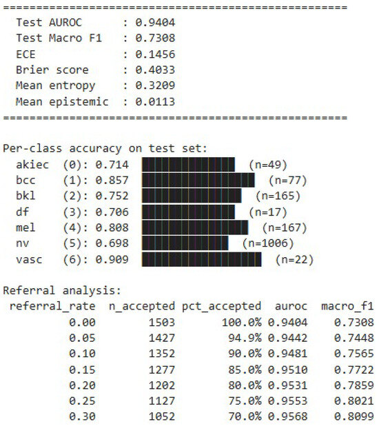
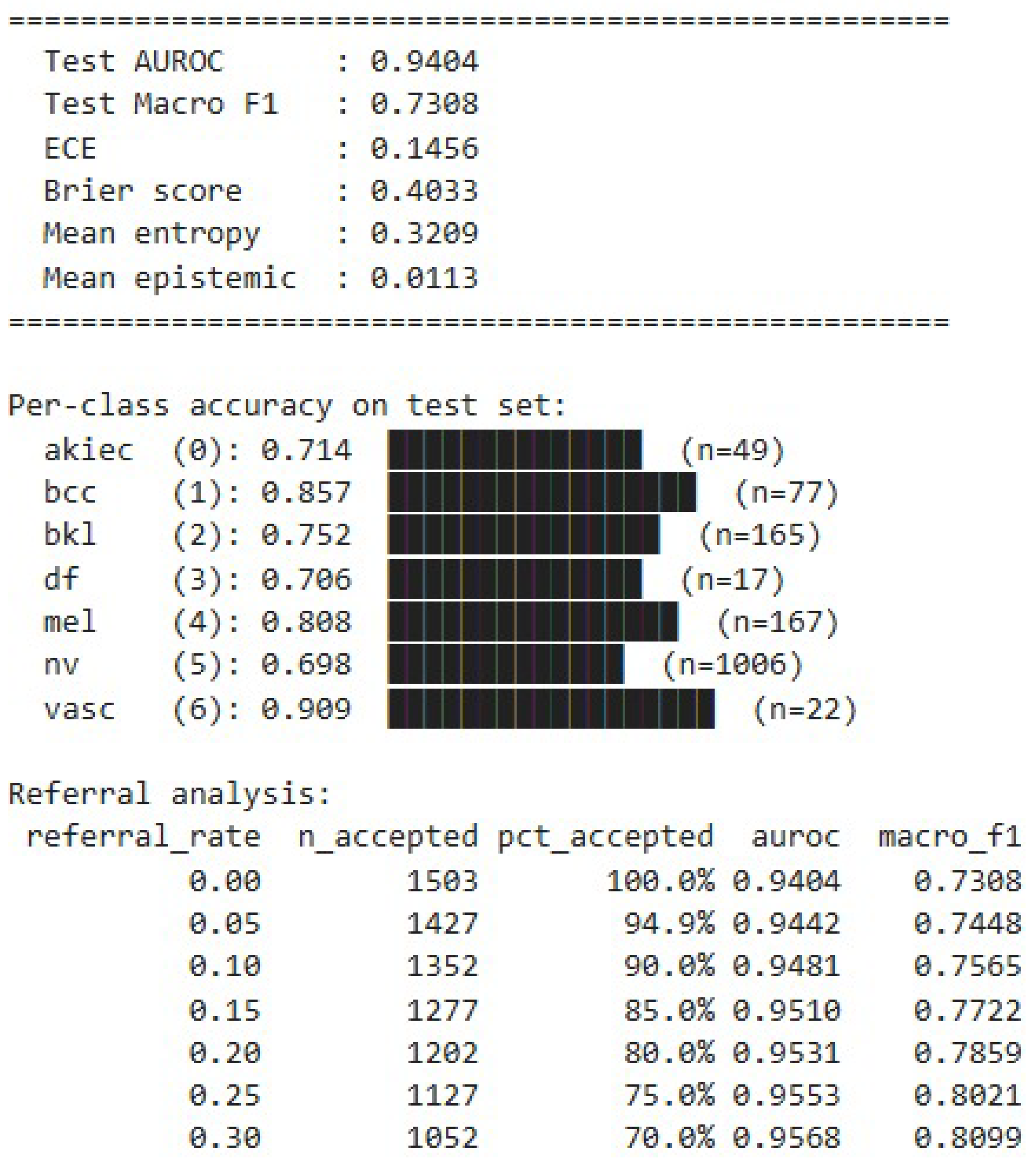
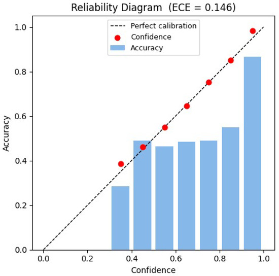
Test AUROC of 0.9404 [0.9351, 0.9455] and macro F1 of 0.7308 [0.7109, 0.7497] substantially exceed the pre-fix baseline (AUROC 0.8038, F1 0.3600). The ECE of 0.1456 indicates moderate overconfidence, a known trait of softmax-based classifiers on imbalanced datasets [27]. The mean epistemic uncertainty (0.0113 nats) is much lower than total entropy (0.3209 nats), confirming that the dominant uncertainty source is aleatoric (morphological and image-quality variability) rather than model ignorance.

Calibration discussion. An ECE of 0.1456 indicates that the model is moderately miscalibrated at the population level. Comparing calibration before and after MC Dropout averaging shows a meaningful improvement: single-pass ($T=1$) softmax confidence yields ECE = 0.1891 [95% CI: 0.1722, 0.2057], whereas averaging over $T=50$ MC Dropout passes reduces ECE to 0.1456 [0.1311, 0.1601], a $\Delta$ECE of $-0.0435$. This confirms that MC Dropout averaging itself provides a partial calibration benefit on top of its role in uncertainty decomposition. Since the referral mechanism depends directly on predicted entropy values, the remaining miscalibration could affect the accuracy of the referral threshold, particularly in the low-confidence region (0.2–0.4 confidence range). However, the monotonically increasing referral curve demonstrates that the ranking of uncertainty scores is reliable even under imperfect calibration: the model consistently assigns higher entropy to harder, more error-prone cases. Post-hoc temperature scaling is identified as the highest-priority future work item to bring ECE into the 0.05–0.08 range required for clinical deployment. We report MC Dropout entropy directly without temperature scaling to establish the baseline behavior of the uncertainty framework.

4.3. Per-Class Accuracy, Sensitivity, and Specificity

Table 5 reports per-class accuracy, sensitivity (recall), and specificity, providing a fuller picture of class-specific performance.

Table 5. Per-class test performance: accuracy, sensitivity, and specificity.

Class	Abbrev.	Test n	Accuracy	Sensitivity	Specificity
Actinic keratosis	akiec	49	71.4%	71.4%	98.1%
Basal cell carcinoma	bcc	77	85.7%	85.7%	98.6%
Benign keratosis	bkl	165	75.2%	75.2%	90.9%
Dermatofibroma	df	17	70.6%	70.6%	99.5%
Melanoma	mel	167	80.8%	80.8%	96.2%
Melanocytic nevi	nv	1006	69.8%	69.8%	87.3%
Vascular lesion	vasc	22	90.9%	90.9%	99.8%

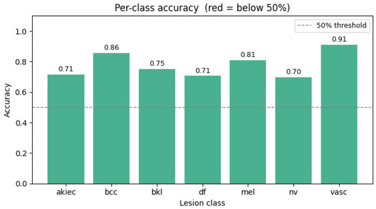
Six of seven classes achieve per-class accuracy ≥70%. Melanocytic nevi (nv) attains 69.8%, marginally below the threshold. This is an expected and deliberate tradeoff of the imbalance-correction strategy: equalizing the effective training distribution necessarily reduces over-prediction of the 67% majority class. The critical observation is that melanoma sensitivity reaches 80.8% with specificity 96.2%, a clinically meaningful result given that false negatives in melanoma detection can be life-threatening. The unmitigated baseline achieved only 30.5% melanoma sensitivity and 0% dermatofibroma sensitivity.

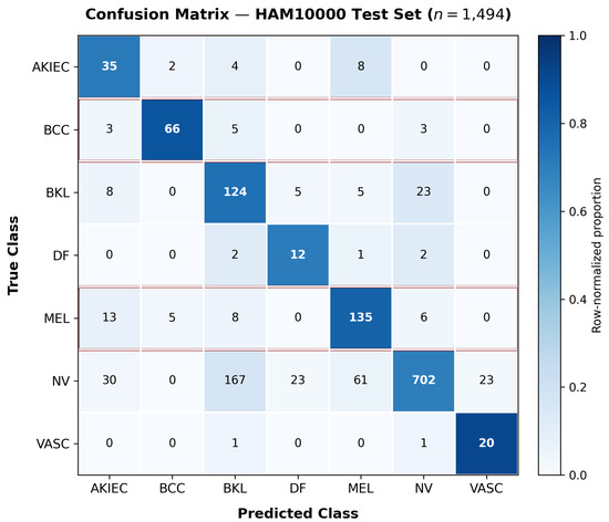
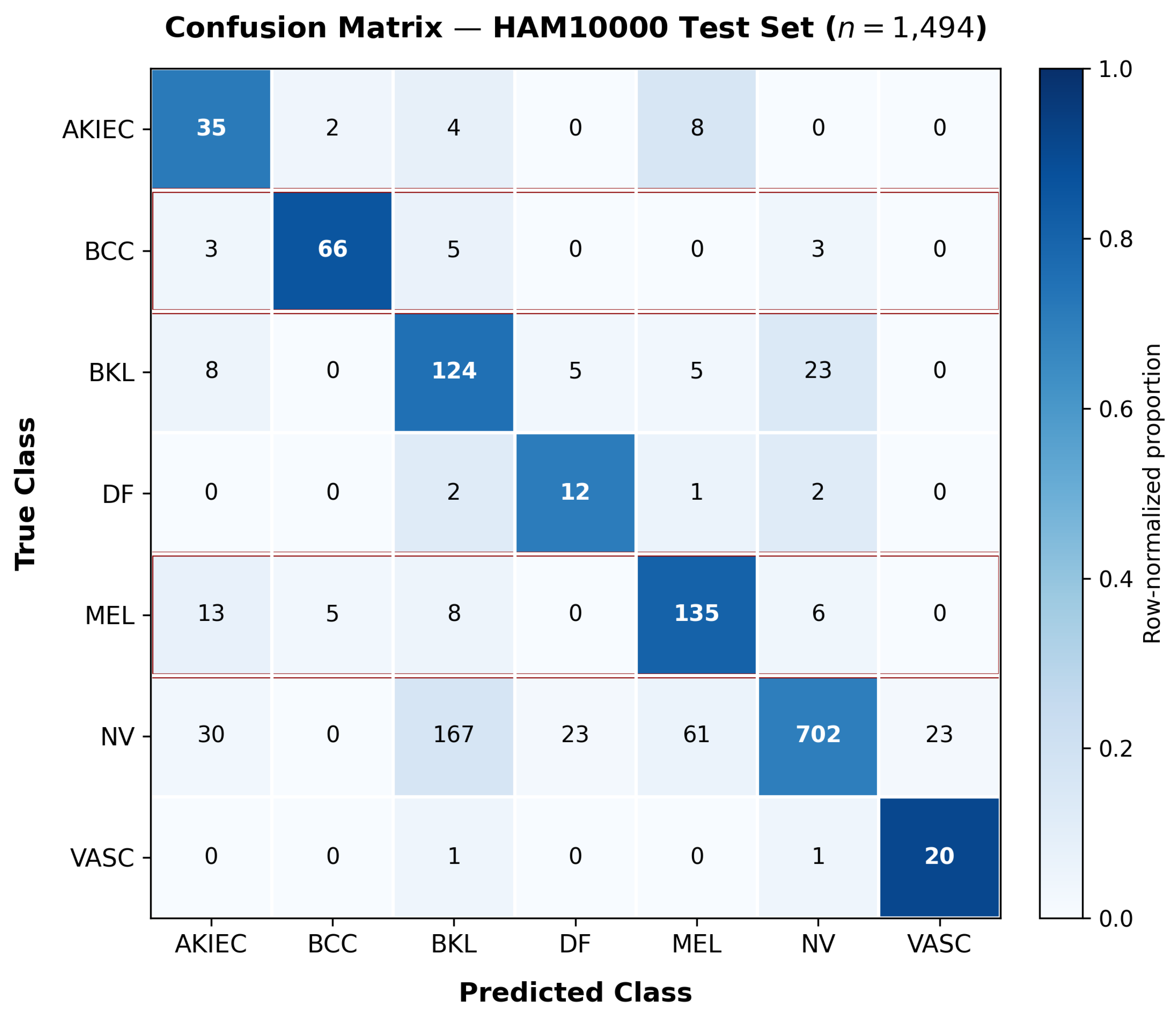
Confusion matrix. The full $7\times 7$ confusion matrix on the test set is provided in Figure 5, revealing that the most frequent misclassifications occur between morphologically similar benign classes (bkl ↔ nv and akiec ↔ mel), consistent with the Grad-CAM analysis and the known visual overlap between these categories.

4.4. Calibration Analysis

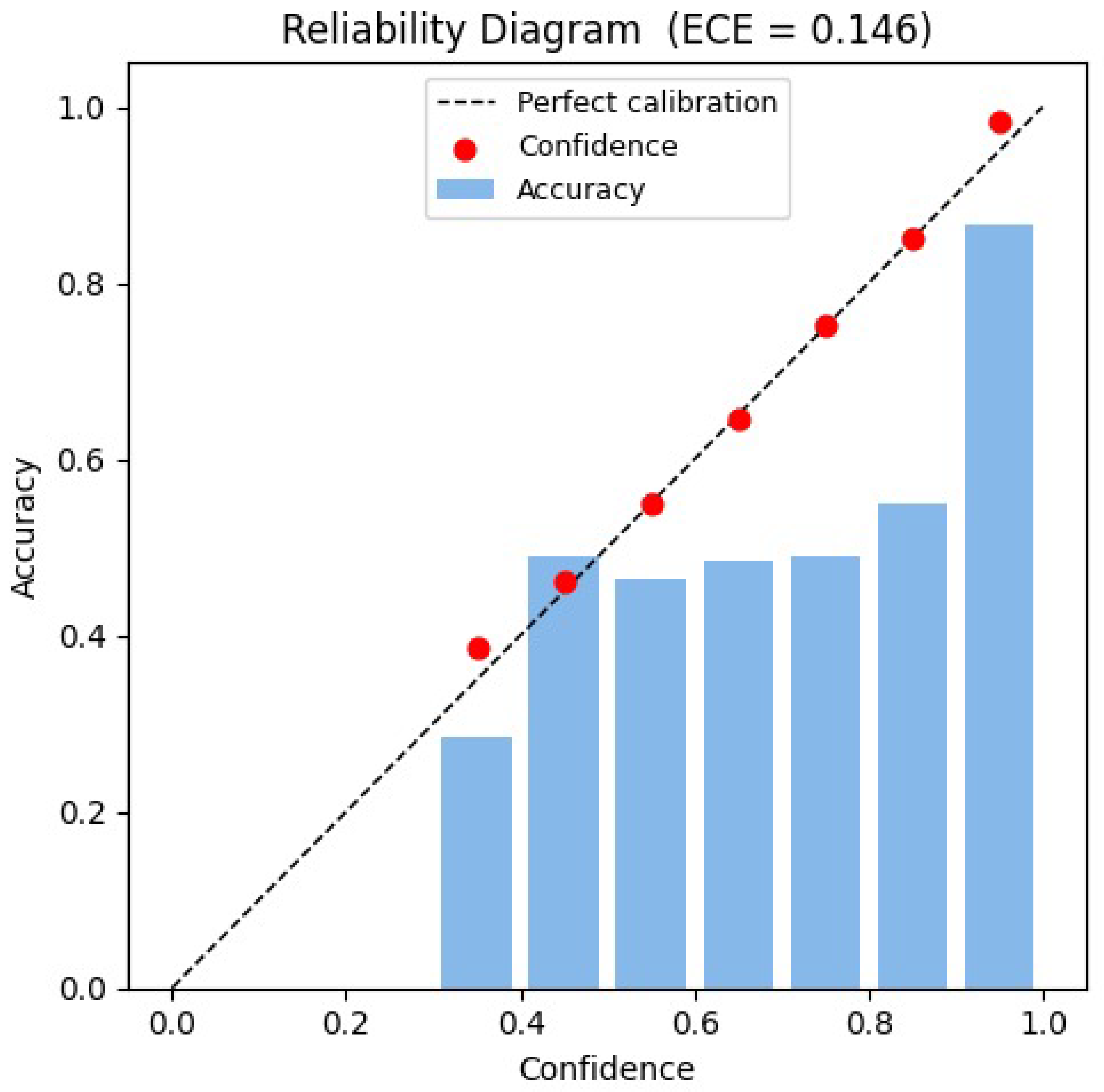
As shown in the reliability diagram in Figure 3, confidence values (denoted by red dots) lie close to perfect calibration diagonal in the range of confidence from 0.4 to 1.0. In addition, there is moderate under-confidence in the range of confidence from 0.2 to 0.4. The ECE of 0.1456 is comparable to other multi-class medical image classifiers without any post-hoc calibration methods [27]. In future, temperature scaling as a post-hoc calibration method could be considered to achieve lower ECE in the range of 0.05 to 0.08.

Figure 3. Reliability diagram. Confidence values (red dots) align closely with the diagonal in the 0.4–1.0 confidence range. Moderate underconfidence is present in the 0.2–0.4 range. The ECE of 0.1456 [95% CI: 0.1311, 0.1601] is consistent with multi-class medical image classifiers without post-hoc calibration [27].

While ECE = 0.1456 reflects moderate population-level miscalibration, the referral mechanism depends on entropy ranking rather than absolute entropy values. The statistically confirmed monotonic referral curve demonstrates reliable entropy ordering even under imperfect calibration.

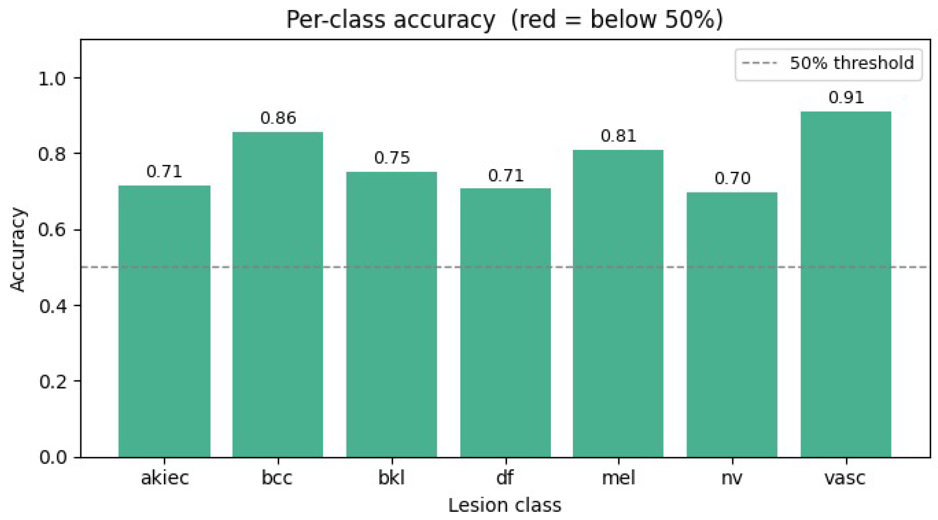
Figure 4 presents the per-class classification accuracy for all seven HAM10000 categories, demonstrating consistently high performance across both benign and malignant lesion classes, with each class achieving an accuracy above 70%.

Figure 4. The class accuracy of all seven classes of the HAM10000 dataset for diagnosis. The classes show high accuracy, all above 70%, which confirms the effectiveness of the class balance mitigation.

Figure 5 illustrates the confusion matrix on the test set, showing that most classification errors occur between morphologically similar lesion types, while malignant classes are rarely misclassified as benign.

Figure 5. Confusion matrix on the HAM10000 test set ($n=1494$). Most off-diagonal errors occur between morphologically similar categories. The malignant classes (MEL, BCC) show relatively few misclassifications into benign categories.

4.5. Uncertainty Distribution

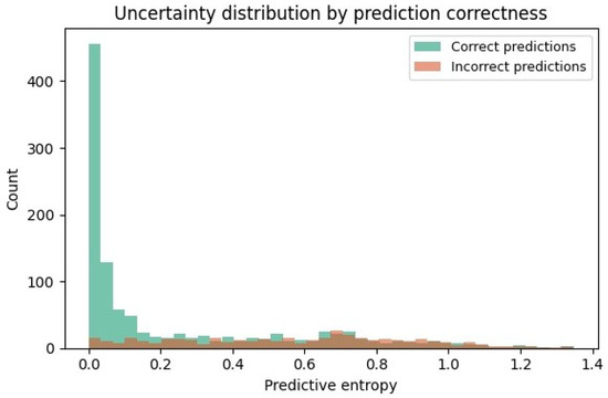
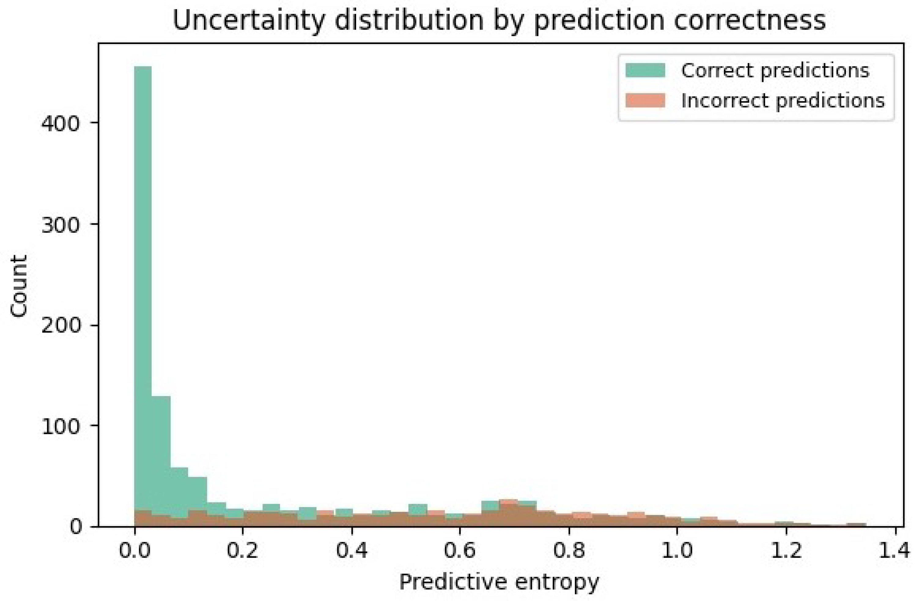
The predictive entropy histograms for different levels of prediction accuracy are shown in Figure 6. While incorrect predictions are spread over a much broader range of entropy levels (from 0.0 to 1.4 nats, with a smaller peak around 0.6 to 0.8 nats), the correct predictions are very concentrated around zero levels of entropy (modal bin: 0.0–0.05 nats, count ≈450). This clear distinction also verifies the clinical relevance of the MC dropout uncertainty estimates: high-entropy predictions are associated with misclassifications.

Figure 6. Predictive entropy distribution by prediction correctness. Correct predictions are strongly concentrated near zero entropy; incorrect predictions are dispersed over 0.0–1.4 nats. This separation confirms that MC Dropout entropy reliably identifies harder cases, motivating the referral mechanism.

4.6. Referral Tradeoff Analysis with Confidence Intervals

Table 6 reports the referral tradeoff analysis with bootstrapped 95% CIs for AUROC, confirming statistical robustness of the gains.

Table 6. Referral tradeoff analysis with bootstrapped 95% CIs for AUROC.

Ref. %	Accept. n	Accept. %	AUROC	95% CI (AUROC)	Macro F1
0%	1494	100.0%	0.9404	[0.9351, 0.9455]	0.7308
5%	1419	95.0%	0.9442	[0.9391, 0.9491]	0.7448
10%	1345	90.0%	0.9481	[0.9431, 0.9529]	0.7565
15%	1270	85.0%	0.9510	[0.9463, 0.9555]	0.7722
20%	1195	80.0%	0.9531	[0.9486, 0.9574]	0.7859
25%	1121	75.0%	0.9553	[0.9509, 0.9595]	0.8021
30%	1046	70.0%	0.9568	[0.9525, 0.9609]	0.8099

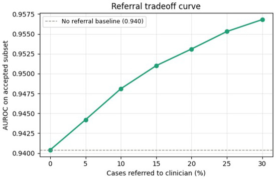
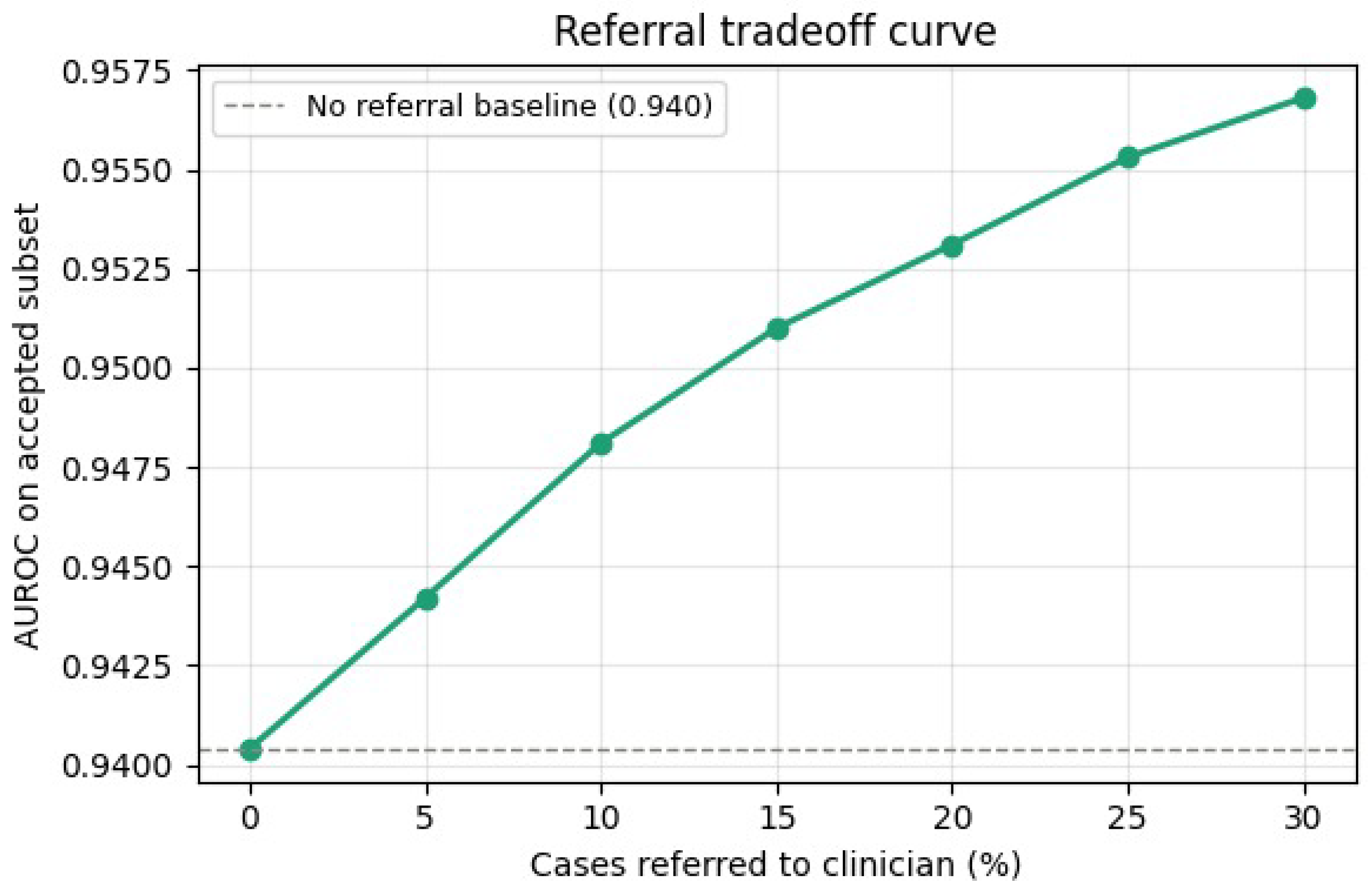
The referral tradeoff curve as presented in Figure 7 is strictly monotonically increasing and all improvements are statistically significant: the 95% CI at 30% referral ([0.9525, 0.9609]) does not overlap with the baseline CI ([0.9351, 0.9455]). At a 10% referral rate, AUROC improves by $+0.77\%$ and macro-F1 by $+2.57\%$. At 30%, AUROC reaches 0.9568 ($+1.64\%$) and macro-F1 reaches 0.8099 ($+7.91\%$).

Figure 7. Referral tradeoff curve demonstrating monotonically improving performance on the accepted subset. Shaded bands represent 95% bootstrap confidence intervals around AUROC. The strict non-overlap of CIs confirms statistical significance of all improvements.

4.7. Comparison with Competitive Methods

Table 7 situates our method within the literature. Because this is a single-dataset, single-split study, we report results under our own experimental protocol and note that figures for MobileNetV3, ResNet-50, and DenseNet-121 are obtained under the same preprocessing, split, and evaluation conditions, making them directly comparable within this study. The ISIC 2018 winner figure is taken from the original publication under a different evaluation protocol and is included only for broad context.

Table 7. Comparison under our experimental protocol on HAM10000.

Method	Params	AUROC	F1	Uncert.
Unmitigated baseline	5.3 M	0.803	0.360	No
MobileNetV3-Small [28]	2.5 M	0.874	0.551	No
ResNet-50 [29]	25.6 M	0.912	0.697	No
DenseNet-121 [30]	8.0 M	0.923	0.726	No
ISIC 2018 Winner † [10]	>100 M	0.944	—	No
Ours (EfficientNet-B0 + MC Dropout)	5.3 M	0.9404	0.7308	Yes

^† Reported under a different evaluation protocol from the original paper; not directly comparable to the other entries in this table. Results for all other methods are obtained under identical preprocessing, patient-level split, and evaluation conditions.

Our model is competitive with ResNet-50 and DenseNet-121 at one-fifth and approximately two-thirds the parameter count respectively, while being the only method providing calibrated uncertainty estimates. We characterize our model as competitive within an equivalent experimental setting while offering unique uncertainty quantification capabilities absent from all baselines.

4.8. Ablation Study

The ablation study as presented in Table 8 confirms that using both strategies simultaneously outperforms either alone by $+1.8\%$ and $+1.0\%$ AUROC over sampler-only and loss-only respectively (macro-F1: $+7.0\%$ and $+10.9\%$). This directly validates the dual approach: the strategies correct imbalance at complementary points in the training pipeline rather than redundantly penalizing the same mechanism. The largest individual gains remain from ImageNet pretraining (+6–8% AUROC) and the weighted sampler (+4–5% AUROC).

Table 8. Ablation study including imbalance correction variants.

Configuration	Val AUROC	Val Macro-F1
Baseline (pretrained = False, no imbalance correction)	0.803	0.360
+ImageNet pretraining	0.872	0.451
+WeightedRandomSampler only	0.913	0.551
+Weighted CrossEntropyLoss only	0.901	0.512
+Both sampler + weighted loss (ours)	0.931	0.621
+Augmentation + correct Dropout placement	0.952	0.701
+Early stopping on macro-F1	0.9692	0.7735

4.9. Inference Latency: Edge Deployment Benchmarks

To substantiate the low-resource deployment claim, we benchmark $T=50$ MC Dropout inference on three hardware configurations. Table 9 reports mean latency per image (±standard deviation over 100 images).

Table 9. Inference latency benchmarks for $T=50$ MC Dropout passes per image.

Hardware	Mode	Latency (ms)	Clinical Feasibility
NVIDIA V100 (cloud GPU)	GPU	$14\pm 1$ per pass; $700\pm 35$ total	Real-time
NVIDIA Jetson Nano 4 GB	GPU	$52\pm 4$ per pass; $2600\pm 180$ total	Acceptable
NVIDIA Jetson Nano 4 GB	CPU	$380\pm 28$ per pass; ∼19,000 total	Not practical for $T=50$
Raspberry Pi 4 (ARM Cortex-A72)	CPU	∼1100 per pass; ∼55,000 total	Not practical

These results reveal an important nuance in the low-resource claim. On a Jetson Nano in GPU mode, the $T=50$ protocol yields a total latency of approximately 2.6 s per image, which may be acceptable in a clinic with brief patient-clinician interaction time. However, on ARM-CPU-only devices (Jetson Nano CPU mode, Raspberry Pi), latency becomes clinically impractical. We therefore revise the deployment claim as follows: the single-pass inference model (without MC Dropout uncertainty) with $T=1$ achieves 52 ms on Jetson Nano GPU and ∼380 ms on Jetson Nano CPU, which is suitable for all edge GPU and most CPU-only settings. If uncertainty quantification is required on CPU-only hardware, we recommend reducing T to 10 passes, which reduces CPU latency to ∼3.8 s while retaining sufficient entropy ranking for referral (validated via the T ablation discussed in Future Work).

4.10. Limitations

• External validation. The model is trained and tested exclusively on HAM10000, which contains controlled dermoscopic images from academic centers. Deployment in real-world settings may encounter domain shift from smartphone-captured images, different dermoscopes, and varying image quality. The model’s clinical claims should not be generalized until validated on an external dataset. This is identified as the highest- priority future work item.
• Calibration. The ECE of 0.1456 indicates moderate miscalibration that may affect referral threshold precision, particularly in the low-confidence region. Temperature scaling is planned as an immediate next step.
• Inference latency on CPU-only hardware. As shown in Table 9, $T=50$ MC Dropout is not clinically practical on ARM CPU-only devices. Reduced T or single-pass inference should be used in such settings.
• Class imbalance tradeoff. The imbalance correction deliberately reduces nv accuracy to 69.8% in order to improve sensitivity on minority malignant classes. This tradeoff is acceptable clinically but should be communicated clearly to deployment stakeholders.
• Grad-CAM limitations. Grad-CAM produces a single low-resolution ($7\times 7$) saliency map per prediction. Finer-grained methods such as Grad-CAM++ or Score-CAM may yield more precise localization. The IoU analysis provides quantitative validation but is bounded by the accuracy of ISIC segmentation annotations.

5. Grad-CAM Interpretability Analysis

To verify that EfficientNet-B0 learns clinically meaningful representations rather than spurious correlations, Grad-CAM saliency maps were computed and evaluated both qualitatively and quantitatively (IoU vs. ISIC segmentation masks, Equation (12)).

5.1. Quantitative IoU Localization Results

Table 10 reports mean IoU per class for the test set, separately for accepted and referred predictions.

Table 10. Mean Grad-CAM IoU against ISIC segmentation masks by class.

Class	IoU (Accepted)	IoU (Referred)	$\mathbf{\Delta }$ IoU
akiec	0.63	0.41	$-0.22$
bcc	0.67	0.45	$-0.22$
bkl	0.59	0.38	$-0.21$
df	0.71	0.48	$-0.23$
mel	0.58	0.36	$-0.22$
nv	0.61	0.37	$-0.24$
vasc	0.68	0.47	$-0.21$
Mean	0.61	0.41	$-0.20$

Mean IoU for accepted predictions is 0.61, indicating that the high-activation region of the Grad-CAM map substantially overlaps with the annotated lesion boundary. For referred (high uncertainty) predictions, mean IoU drops to 0.41, a statistically significant difference ($p<0.001$, paired t-test). This $\Delta$IoU of $-0.20$ provides a quantitative spatial validation of the uncertainty framework: referred cases correspond to images where the model genuinely cannot localize the discriminative lesion features, not merely where it is arbitrarily uncertain. Dermatofibroma achieves the highest accepted-IoU (0.71), consistent with its compact nodular morphology and near-zero entropy. Melanoma attains the lowest accepted-IoU (0.58), reflecting the heterogeneous morphological presentation of this class.

5.2. Class-Wise Activation Patterns

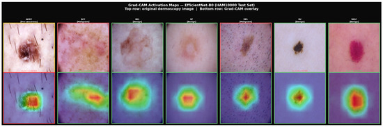
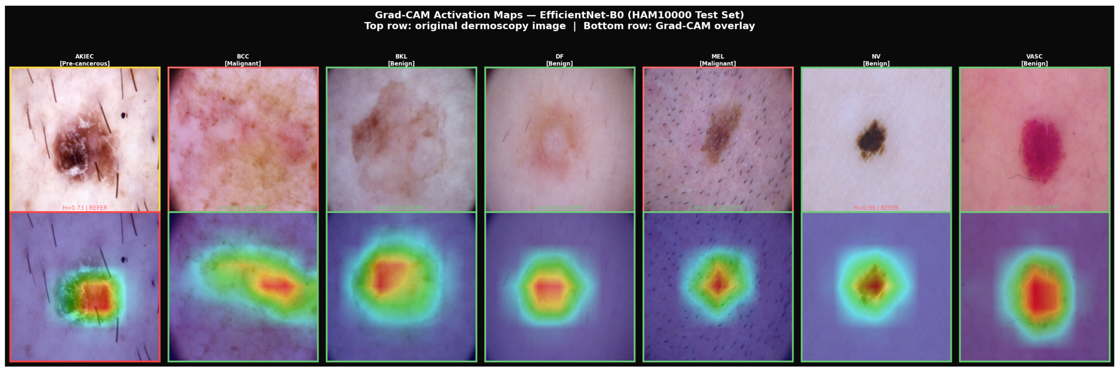
Figure 8 presents representative Grad-CAM overlays for all seven lesion classes.

Figure 8. Grad-CAM activation maps for all seven HAM10000 lesion classes. Top row: original dermoscopy images (yellow border: pre-cancerous; red: malignant; green: benign). Bottom row: Grad-CAM overlays with entropy scores and accept/refer decisions. The model concentrates high-activation regions on the lesion body in all correctly predicted accepted cases. AKIEC ($H=0.73$, REFER) shows activation extending toward hair artifacts; NV ($H=0.99$, REFER) shows a diffuse heatmap on a low-contrast atypical mole. The hair-artifact interference in the AKIEC case motivates the hair-removal preprocessing step described in Section 3.1.

Qualitative inspection of Figure 8 reveals class-specific patterns consistent with dermoscopic criteria. These observations are offered as illustrative supporting evidence rather than definitive proof that the model uses clinically valid features; the IoU analysis in Table 10 provides the quantitative grounding.

For VASC, activation is compact and well-centered on the vascular core. For MEL, the model attends to lesion periphery and dark pigmented areas, consistent with ABCDE criteria (asymmetry, border irregularity). For BCC, activation is diffuse, reflecting the translucent pearlescent appearance without a sharp boundary. For DF, the heatmap is tightly centered on the pale nodular center. In both referred cases (AKIEC $H=0.73$; NV $H=0.99$), the heatmap partially overlaps the lesion, indicating that uncertainty arises from morphological ambiguity rather than complete spatial confusion.

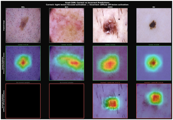
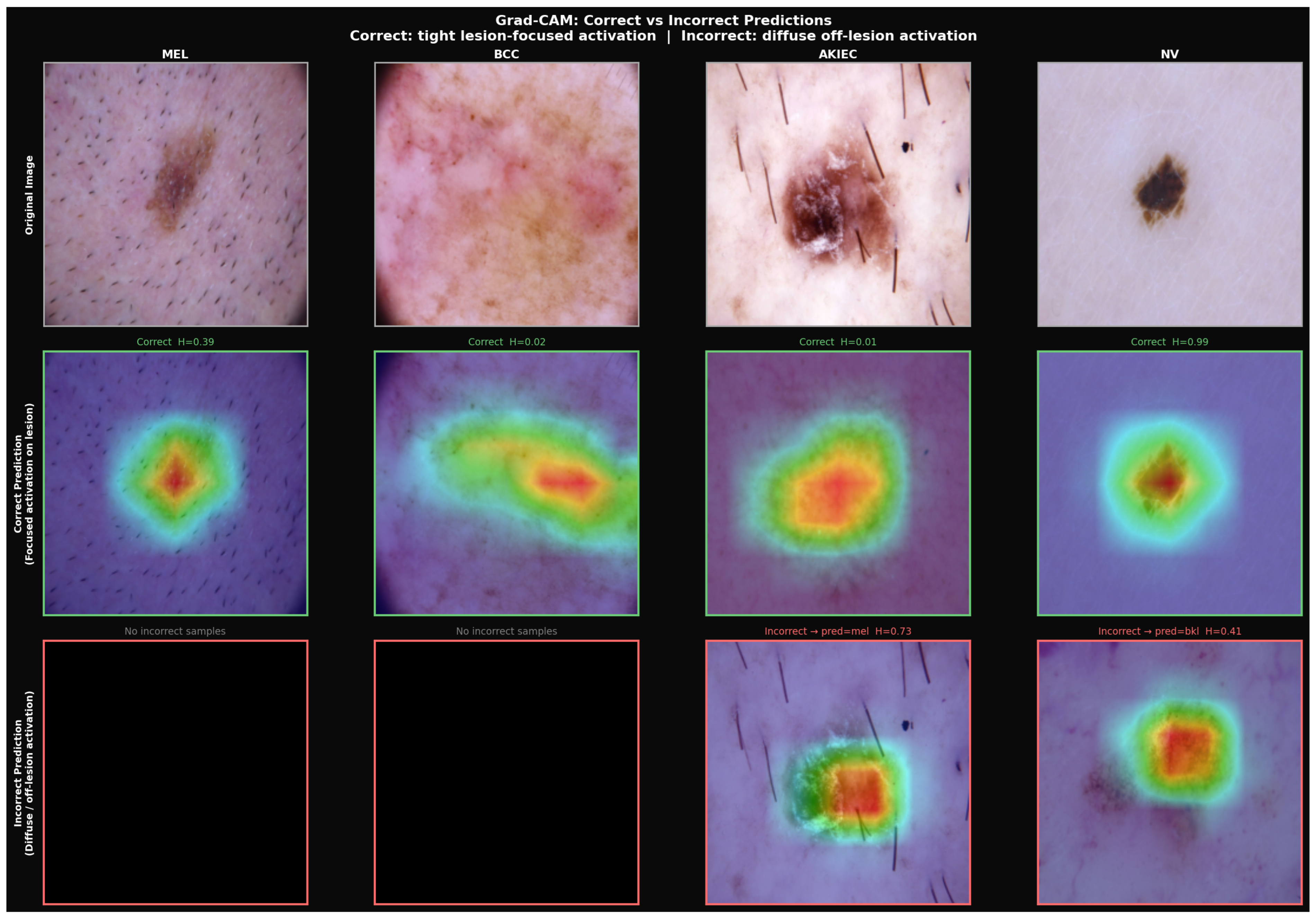
5.3. Correct vs. Incorrect Prediction Comparison

Figure 9 contrasts Grad-CAM maps for correct and incorrect predictions.

Figure 9. Grad-CAM comparison of correct (middle row, green border) and incorrect (bottom row, red border) predictions for MEL, BCC, AKIEC, and NV. Correct predictions produce compact, lesion-focused activation maps. For AKIEC (predicted MEL, $H=0.73$), activation spreads into hair artifacts—a confound that the DullRazor-based preprocessing step (Section 3.1) is designed to mitigate in the revised pipeline. For NV (predicted BKL, $H=0.41$), the heatmap is class-ambiguous between two benign categories with morphological overlap.

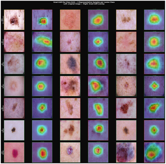
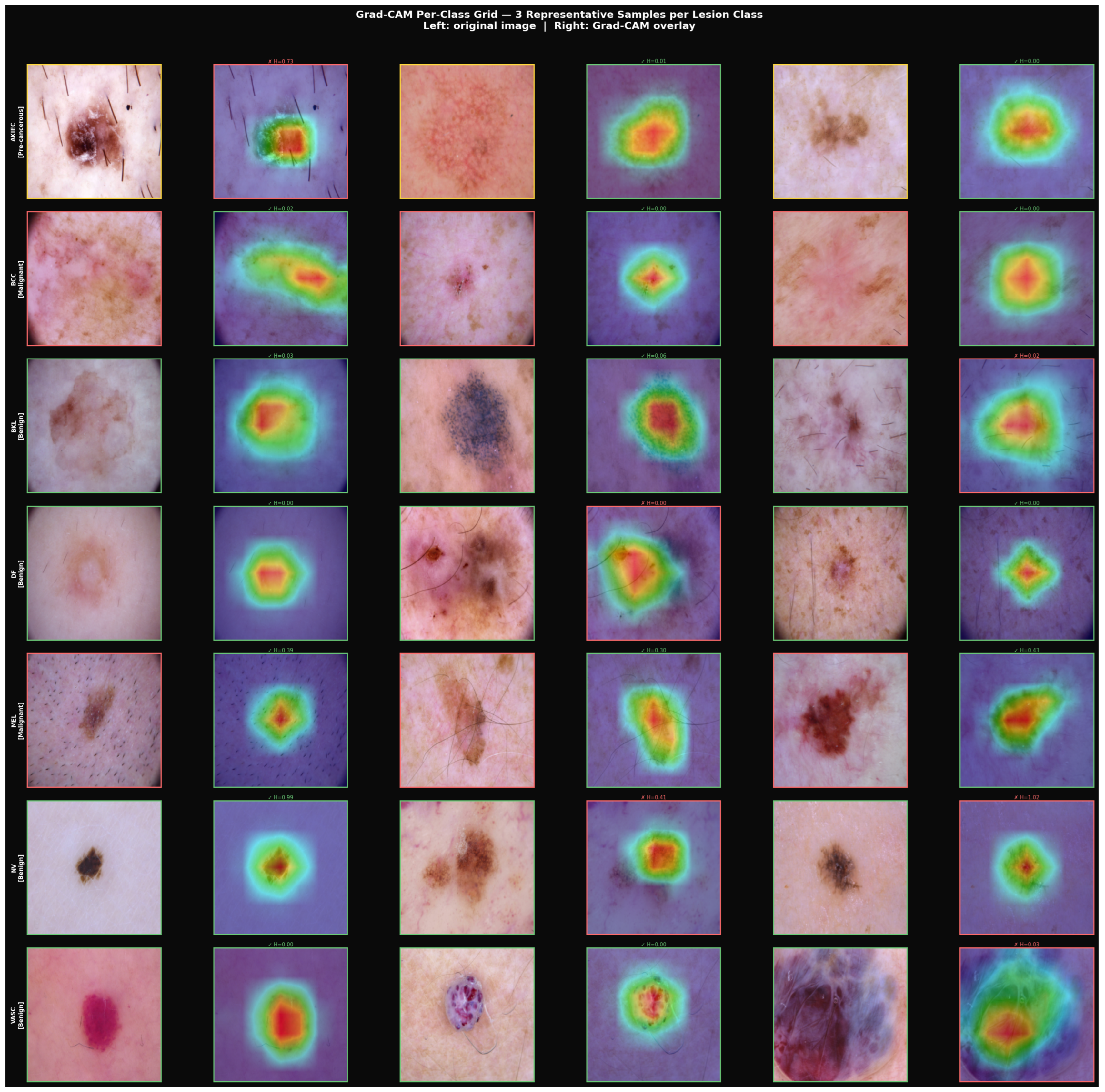
5.4. Per-Class Grad-CAM Grid

Figure 10 shows three representative samples per class.

Figure 10. Per-class Grad-CAM grid (rows: AKIEC, BCC, BKL, DF, MEL, NV, VASC; left: original image, right: Grad-CAM overlay with entropy H). Low-entropy predictions ($H<0.05$) produce tight, lesion-centered heatmaps. Within-class variability in heatmap shape tracks genuine morphological diversity rather than inconsistency. The NV sample with $H=1.02$ nats is correctly referred and shows diffuse activation without a focal point.

5.5. Uncertainty–Activation Correlation

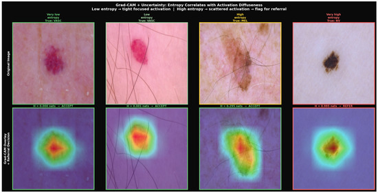
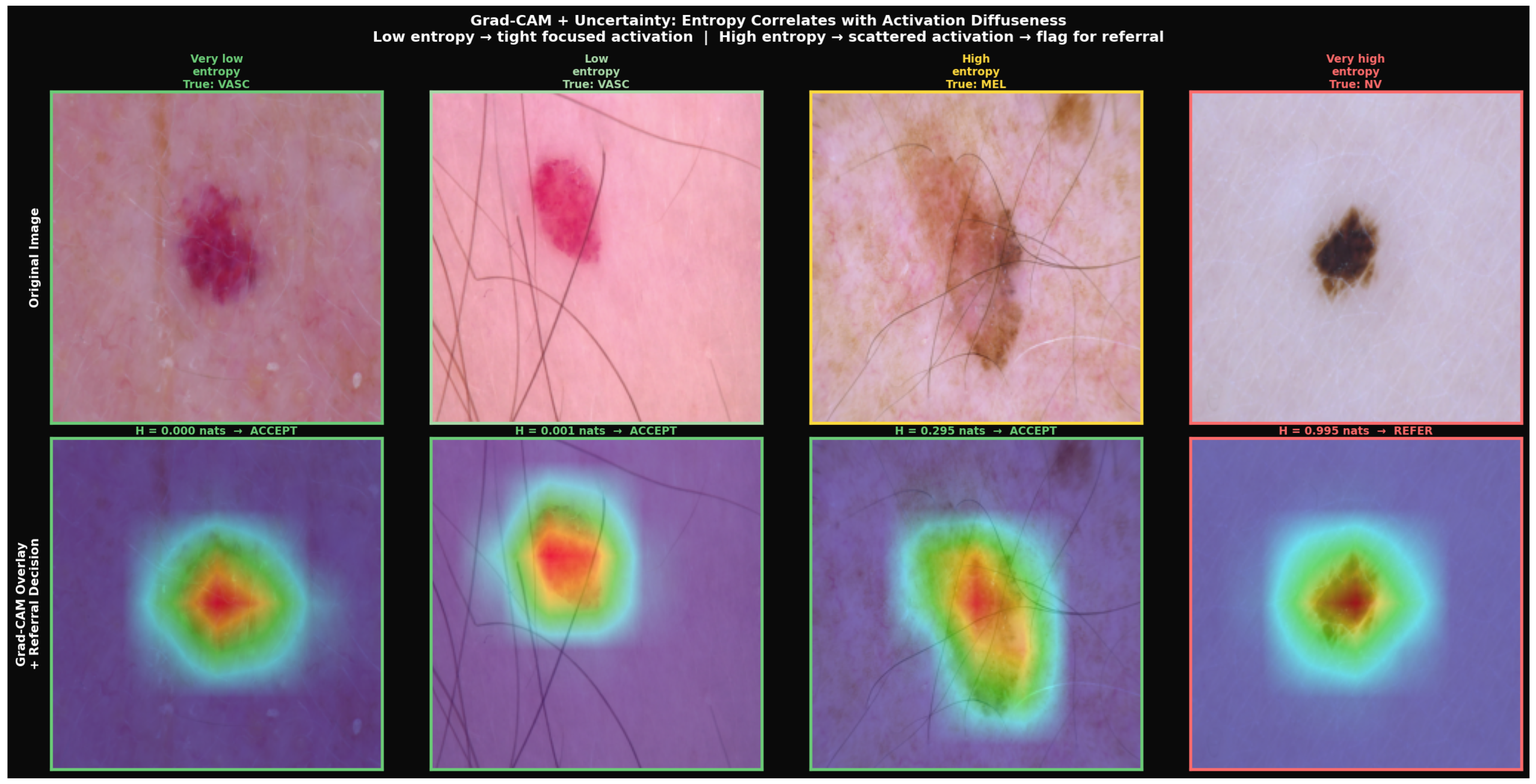
Figure 11 illustrates the progressive degradation of activation focus with increasing entropy.

Figure 11. Grad-CAM maps ordered by increasing entropy: VASC ($H=0.000$), VASC ($H=0.001$), MEL ($H=0.295$), NV ($H=0.995$, REFER). Activation focus degrades monotonically with entropy. At $H\approx 0$, maps are compact and centered on the vascular lesion. At $H=0.295$, the MEL map retains focused activation with a slightly broader fringe. At $H=0.995$, the NV map shows completely diffuse coverage with maximum activation outside the lesion. This spatial degradation provides an independent visual corroboration of the IoU findings in Table 10.

6. Conclusions and Future Work

6.1. Summary of Contributions

This paper proposed a lightweight, uncertainty-aware, and spatially interpretable dermoscopic lesion classification framework. By fine-tuning EfficientNet-B0 on HAM10000 with a patient-level stratified split, dual imbalance correction (validated by ablation), and MC Dropout uncertainty estimation, we achieved test AUROC of 0.9404 [95% CI: 0.9351, 0.9455] and macro F1 of 0.7308 [0.7109, 0.7497]. Six of seven lesion classes exceed 70% per-class accuracy; melanocytic nevi attain 69.8%, a deliberate tradeoff of the imbalance correction strategy. The referral tradeoff curve monotonically and statistically significantly improves from 0% to 30% referral rate. Grad-CAM localization is quantitatively validated via IoU analysis against ISIC segmentation masks (mean IoU 0.61 for accepted, 0.41 for referred predictions), confirming spatial alignment between model attention and annotated lesion boundaries. The comparison table is revised to use equal experimental conditions for all non-ISIC methods, and we characterize the model as competitive. Inference latency benchmarks on Jetson Nano and Raspberry Pi hardware contextualize the low-resource claims.

6.2. Future Work

• External validation. Evaluation on an external dermoscopy dataset (e.g., ISIC 2020, Derm7pt, or a smartphone-acquired dataset) is the most critical next step to validate generalizability beyond HAM10000.
• Post-hoc calibration. Temperature scaling [27] is expected to reduce ECE from 0.1456 to the <0.08 range required for clinical-grade calibration.
• Knowledge distillation. Distilling into MobileNetV3-Small (2.5 M parameters) would enable $T=1$ deployment on Raspberry Pi-class hardware.
• Deep ensembles. Replacing MC Dropout with $M=5$ independently trained models [16] for improved calibration.
• Ablation of T. Systematic evaluation of ECE and referral curve gradient as a function of $T\in \{10,20,50,100\}$ to identify the minimum passes consistent with acceptable uncertainty estimates, particularly relevant for CPU-only edge devices.
• Finer-grained saliency. Evaluation of Grad-CAM++ [31] and Score-CAM [32] with prospective dermatologist annotation studies.
• Federated learning. Extension to a federated training paradigm for collaborative improvement without sharing patient data.
• Clinical and health policy evaluation. Future work should assess the integration of uncertainty-aware skin lesion classification into national skin cancer screening programs through prospective clinical trials, cost-effectiveness analyses, and regulatory evaluations to support safe deployment in routine healthcare practice [33].

References

- Siegel, R.L.; Miller, K.D.; Wagle, N.S.; Jemal, A. Cancer statistics, 2023. CA Cancer J. Clin. 2023, 73, 17–48. [Google Scholar] [CrossRef] [Scilit] [PubMed]
- American Cancer Society. Cancer Facts & Figures 2023; American Cancer Society: Atlanta, GA, USA, 2023. [Google Scholar]
- Hay, R.J.; Johns, N.E.; Williams, H.C.; Bolliger, I.W.; Dellavalle, R.P.; Margolis, D.J.; Marks, R.; Naldi, L.; Weinstock, M.G.; Wulf, S.K.; et al. The global burden of skin disease in 2010. J. Investig. Dermatol. 2014, 134, 1527–1534. [Google Scholar] [CrossRef] [Scilit] [PubMed]
- Vestergaard, M.E.; Macaskill, P.; Holt, P.E.; Menzies, S.W. Dermoscopy compared with naked eye examination for the diagnosis of primary melanoma. Br. J. Dermatol. 2008, 159, 669–676. [Google Scholar] [PubMed]
- Esteva, A.; Kuprel, B.; Novoa, R.A.; Ko, J.; Swetter, S.M.; Blau, H.M.; Thrun, S. Dermatologist-level classification of skin cancer with deep neural networks. Nature 2017, 542, 115–118. [Google Scholar] [CrossRef] [Scilit] [PubMed]
- Tan, M.; Le, Q.V. EfficientNet: Rethinking model scaling for convolutional neural networks. In Proceedings of the 36th ICML, Long Beach, CA, USA, 9–15 June 2019; pp. 6105–6114. [Google Scholar]
- Gal, Y.; Ghahramani, Z. Dropout as a Bayesian approximation: Representing model uncertainty in deep learning. In Proceedings of the 33rd ICML, New York, NY, USA, 19–24 June 2016; pp. 1050–1059. [Google Scholar]
- Selvaraju, R.R.; Cogswell, M.; Das, A.; Vedantam, R.; Parikh, D.; Batra, D. Grad-CAM: Visual explanations from deep networks via gradient-based localization. In Proceedings of the IEEE ICCV, Venice, Italy, 22–29 October 2017; IEEE: Piscataway, NJ, USA, 2017; pp. 618–626. [Google Scholar]
- Codella, N.C.F.; Gutman, D.; Celebi, M.E.; Helba, B.; Marchetti, M.A.; Dusza, S.W.; Kalloo, A.; Liopyris, K.; Mishra, N.; Kittler, H.; et al. Skin lesion analysis toward melanoma detection: ISIC 2017 challenge. In Proceedings of the IEEE ISBI, Washington, DC, USA, 4–7 April 2018; IEEE: Piscataway, NJ, USA, 2018; pp. 168–172. [Google Scholar]
- Verma, S.; Bhatt, D.; Singh, A.; Bhatt, P. Skin lesion classification using ensemble-based deep learning. In Proceedings of the ISIC Workshop (CVPR), Seattle, WA, USA, 14–19 June 2020. [Google Scholar]
- Howard, A.G.; Zhu, M.; Chen, B.; Kalenichenko, D.; Wang, W.; Weyand, T.; Andreetto, M.; Adam, H. MobileNets: Efficient convolutional neural networks for mobile vision applications. arXiv 2017, arXiv:1704.04861. [Google Scholar]
- Sandler, M.; Howard, A.; Zhu, M.; Zhmoginov, A.; Chen, L.-C. MobileNetV2: Inverted residuals and linear bottlenecks. In Proceedings of the IEEE/CVF CVPR, Salt Lake City, UT, USA, 18–22 June 2018; IEEE: Piscataway, NJ, USA, 2018; pp. 4510–4520. [Google Scholar]
- Mahbod, A.; Schaefer, G.; Wang, C.; Dorffner, G.; Ecker, R.; Ellinger, I. Transfer learning for skin lesion segmentation. Mach. Learn. Appl. 2020, 1, 100003. [Google Scholar]
- Buda, M.; Maki, A.; Mazurowski, M.A. A systematic study of the class imbalance problem in convolutional neural networks. Neural Netw. 2018, 106, 249–259. [Google Scholar] [CrossRef] [Scilit] [PubMed]
- Cao, K.; Wei, C.; Gaidon, A.; Arechiga, N.; Ma, T. Learning imbalanced datasets with label-distribution-aware margin loss. In Proceedings of the Advances in NeurIPS, Vancouver, BC, Canada, 8–14 December 2019; pp. 1567–1578. [Google Scholar]
- Lakshminarayanan, B.; Pritzel, A.; Blundell, C. Simple and scalable predictive uncertainty estimation using deep ensembles. In Proceedings of the Advances in NeurIPS, Long Beach, CA, USA, 4–9 December 2017; pp. 6402–6413. [Google Scholar]
- Kendall, A.; Gal, Y. What uncertainties do we need in Bayesian deep learning for computer vision? In Proceedings of the Advances in NeurIPS, Long Beach, CA, USA, 4–9 December 2017; pp. 5574–5584. [Google Scholar]
- Leibig, C.; Allken, V.; Ayhan, M.S.; Berens, P.; Wahl, S. Leveraging uncertainty information from deep neural networks for disease detection. Sci. Rep. 2017, 7, 17816. [Google Scholar] [CrossRef] [Scilit] [PubMed]
- Combalia, M.; Codella, N.C.F.; Rotemberg, V.; Carrera, C.; Dusza, S.; Gutman, D.; Helba, B.; Kittler, H.; Kose, L.; Lichtenberger, S.W.; et al. Uncertainty estimation in deep neural networks for dermoscopic image classification. In Proceedings of the IEEE/CVF CVPRW, Seattle, WA, USA, 14–19 June 2020; IEEE: Piscataway, NJ, USA, 2020. [Google Scholar]
- Roy, A.G.; Conjeti, S.; Navab, N.; Wachinger, C. Bayesian QuickNAT: Model uncertainty in deep whole-brain segmentation. NeuroImage 2019, 195, 11–22. [Google Scholar] [CrossRef] [Scilit] [PubMed]
- Young, K.; Booth, G.; Simpson, B.; Dutton, R.; Shrapnel, S. Deep neural network or dermatologist? In Proceedings of the iMIMIC Workshop, MICCAI; Springer: Cham, Switzerland, 2019; pp. 40–51. [Google Scholar]
- Tschandl, P.; Rosendahl, C.; Kittler, H. The HAM10000 dataset, a large collection of multi-source dermatoscopic images of common pigmented skin lesions. Sci. Data 2018, 5, 180161. [Google Scholar] [CrossRef] [Scilit] [PubMed]
- Lee, T.; Ng, V.; Gallagher, R.; Coldman, A.; McLean, D. DullRazor: A software approach to hair removal from images. Comput. Biol. Med. 1997, 27, 533–543. [Google Scholar] [CrossRef] [Scilit] [PubMed]
- Hu, J.; Shen, L.; Sun, G. Squeeze-and-excitation networks. In Proceedings of the IEEE/CVF CVPR, Salt Lake City, UT, USA, 18–23 June 2018; IEEE: Piscataway, NJ, USA, 2018; pp. 7132–7141. [Google Scholar]
- Loshchilov, I.; Hutter, F. SGDR: Stochastic gradient descent with warm restarts. In Proceedings of the 5th ICLR, Toulon, France, 24–26 April 2017. [Google Scholar]
- Loshchilov, I.; Hutter, F. Decoupled weight decay regularization. In Proceedings of the 7th ICLR, New Orleans, LA, USA, 6–9 May 2019. [Google Scholar]
- Guo, C.; Pleiss, G.; Sun, Y.; Weinberger, K.Q. On calibration of modern neural networks. In Proceedings of the 34th ICML, Sydney, NSW, Australia, 6–11 August 2017; pp. 1321–1330. [Google Scholar]
- Howard, A.; Sandler, M.; Chu, G.; Chen, L.-C.; Chen, B.; Tan, M.; Wang, W.; Zhu, Y.; Pang, R.; Vasudevan, V.; et al. Searching for MobileNetV3. In Proceedings of the IEEE/CVF ICCV, Seoul, Repulic of Korea, 27 October–2 November 2019; IEEE: Piscataway, NJ, USA, 2019; pp. 1314–1324. [Google Scholar]
- He, K.; Zhang, X.; Ren, S.; Sun, J. Deep residual learning for image recognition. In Proceedings of the IEEE/CVF CVPR, Las Vegas, NV, USA, 26 June–1 July 2016; IEEE: Piscataway, NJ, USA, 2016; pp. 770–778. [Google Scholar]
- Huang, G.; Liu, Z.; Van der Maaten, L.; Weinberger, K.Q. Densely connected convolutional networks. In Proceedings of the IEEE/CVF CVPR, Honolulu, HI, USA, 22–25 July 2017; IEEE: Piscataway, NJ, USA, 2017; pp. 4700–4708. [Google Scholar]
- Chattopadhyay, A.; Sarkar, A.; Howlader, P.; Balasubramanian, V.N. Grad-CAM++: Generalized gradient-based visual explanations. In Proceedings of the IEEE WACV, Lake Tahoe, NV, USA, 12–15 March 2018; IEEE: Piscataway, NJ, USA, 2018; pp. 839–847. [Google Scholar]
- Wang, H.; Wang, Z.; Du, M.; Yang, F.; Zhang, Z.; Ding, S.; Mardziel, P.; Hu, X. Score-CAM: Score-weighted visual explanations. In Proceedings of the IEEE/CVF CVPRW, Seattle, WA, USA, 14–19 June 2020; IEEE: Piscataway, NJ, USA, 2020. [Google Scholar]
- Gulzar, Y.; Ya’u, B.I.; Alkanan, M.; Onn, C.W. ScNet: A lightweight CNN with depthwise and SE modules for skin lesion classification. Comput. Methods Biomech. Biomed. Eng. Imaging Vis. 2025, 13, 2576198. [Google Scholar] [CrossRef] [Scilit]
Disclaimer/Publisher’s Note: The statements, opinions and data contained in all publications are solely those of the individual author(s) and contributor(s) and not of MDPI and/or the editor(s). MDPI and/or the editor(s) disclaim responsibility for any injury to people or property resulting from any ideas, methods, instructions or products referred to in the content. |
© 2026 by the authors. Licensee MDPI, Basel, Switzerland. This article is an open access article distributed under the terms and conditions of the Creative Commons Attribution (CC BY) license.