Comparison of Shoreline Determination Methods Using Multi-Sensor Data in Low-Relief Coastal Environments

Abstract

Shoreline determination is fundamental to coastal research, spatial planning, and legal boundary delineation but remains challenging in low-relief coastal areas where small sea-level variations can produce substantial horizontal shoreline displacements. This study compares shoreline determination methods based on tide gauge (TG) observations, LiDAR data, Sentinel-1 synthetic aperture radar (SAR) and Sentinel-2 optical satellite imagery using the low-relief coast of Pärnu Bay, Estonia, as a case study. The comparison was based on shorelines derived from Sentinel-1 and Sentinel-2 imagery acquired on selected common acquisition dates within the 2015–2025 study period, rather than on a temporally continuous annual dataset, and compared with temporally matched LiDAR-derived shorelines extracted from a Digital Terrain Model (DTM) generated from a 2021 LiDAR survey. The LiDAR-derived shorelines were extracted using the mean sea level (MSL) observed at the Pärnu and Häädemeeste TGs at the satellite overpass time, while the satellite-derived shorelines were additionally validated against RTK GNSS measurements. The results demonstrate that the evaluated methods produce substantially different shoreline positions. Sentinel-2-derived shorelines generally corresponded more closely to the temporally matched LiDAR-derived shorelines than Sentinel-1-derived shorelines and most accurately represented the instantaneous land–water boundary during field validation. These findings demonstrate that different shoreline determination methods represent different shoreline definitions. Consequently, shoreline datasets should be interpreted according to their intended purpose rather than treated as directly interchangeable.

1. Introduction

The shoreline is one of the most important spatial boundaries serving as a fundamental reference for the analysis of coastal processes, coastal management, habitat mapping, and spatial planning. In addition to its geomorphological and environmental significance, the shoreline also has important legal implications. It forms the basis for the delimitation of a state’s territorial sea and other maritime zones, the establishment of land-use restrictions, and the determination of property boundaries. Consequently, the choice of shoreline definition may influence both scientific analyses and legal or administrative decisions. Despite its apparent simplicity, the shoreline is neither fixed nor unambiguously defined; rather, it is a dynamic interface between land and sea, the position of which changes over time in response to hydrodynamic processes, sediment transport, and sea-level variability [1].

One of the central challenges in shoreline mapping is the absence of a universally accepted definition of the shoreline. Historically, shorelines have been defined on the basis of both geomorphological indicators and sea-level reference surfaces. Traditional approaches relied on features such as beach ridges, erosion scarps, or vegetation limits, whereas modern approaches increasingly define the shoreline using statistically derived sea-level elevations [1,2].

Internationally, shoreline determination depends on both the selected statistical sea-level reference and the data sources used. The legal significance of the shoreline arises from its role in delineating various marine and terrestrial boundaries, including territorial sea baselines, coastal construction setback zones, flood-prone areas, and the boundary between private land parcels and public water bodies. Practices vary among countries; for example, in Estonia, the official national shoreline is associated with mean sea level (MSL), whereas in New Zealand, mean high water springs (MHWS) serves as a principal planning boundary. MSL is commonly used as a geodetic reference surface representing the long-term average sea level. Different vertical reference data lead to systematic differences in the mapped shoreline position [1].

In the United States, the shoreline is commonly referenced to the Mean High Water (MHW) level, which is determined from long-term tidal records and projected into the national vertical datum (NAVD88). This reference serves as a basis for both coastal management and national shoreline change monitoring programs [3]. In contrast, Canada and the Netherlands widely employ digital elevation models derived from LiDAR data for shoreline mapping, coastal management, and flood risk assessment [4]. In Australia and the United Kingdom, optical satellite imagery is frequently used in combination with spectral indices such as the Normalized Difference Water Index (NDWI) to extract the instantaneous land–water boundary, which is subsequently interpreted relative to a tidal or sea-level reference datum [5].

Examples of the principal shoreline reference frameworks adopted in different countries are summarized in Table 1.

Table 1. Examples of shoreline reference frameworks adopted in different countries.

Country	Shoreline Reference	Typical Application
Estonia	Mean Sea Level (MSL)	National reference shoreline, spatial planning
United States	Mean High Water (MHW)	Coastal management, legal shoreline, shoreline change monitoring
New Zealand	Mean High Water Springs (MHWS)	Coastal planning and legal boundaries
Canada	LiDAR-derived shoreline referenced to the national vertical datum	Shoreline mapping, flood risk assessment
Netherlands	LiDAR-derived shoreline referenced to the national vertical datum	Coastal management and flood protection
Australia/United Kingdom	Instantaneous shoreline from optical imagery	Coastal monitoring and shoreline mapping

Consequently, contemporary approaches increasingly rely on remote sensing data from which the instantaneous land–water boundary can be extracted. Each approach reflects a particular conceptual understanding of the shoreline and is inherently linked to the characteristics, spatial resolution, and vertical reference of the data used. The selected vertical reference directly determines shoreline position and affects the comparability of results obtained using different methods. As a result, shorelines determined using different approaches are often not directly comparable, even when they describe the same coastal segment [3]. This has long posed challenges both for the assessment of shoreline change and for legal applications, where differing shoreline definitions may lead to the delineation of different boundaries.

Recent technological advances have shifted shoreline mapping from visually interpreted and inherently subjective approaches towards automated and vertically controlled methods. LiDAR, synthetic aperture radar (SAR) and optical remote sensing, satellite altimetry, aerial photogrammetry, digital image processing, and machine learning have considerably improved the accuracy and consistency of shoreline determination. In contemporary international practice, two principal approaches to shoreline determination can be distinguished: (i) the geodetic shoreline, which is based on a geodetic sea-level reference, and (ii) the instantaneous land–water boundary extracted from remote sensing data.

The Baltic Sea is characterized by a very small tidal range, amounting to only about 2–5 cm in most regions, reaching up to 10 cm in the Gulf of Finland and 15–30 cm in the Danish Straits [6]. In contrast, short-term sea-level variability is substantial, with storm surges typically raising sea level by 1–2 m and, in extreme cases, by more than 2 m [7,8,9]. Sea-level fluctuations are primarily driven by wind forcing and atmospheric pressure gradients [6,10,11]. In addition, the instantaneous position of the shoreline is influenced by storms, wave action, and sea-level extremes. The occurrence of successive cyclones may generate cumulative high-water episodes and intensify coastal processes, particularly along low-gradient coastal sections [12,13]. These factors make shoreline definition highly sensitive to temporal variability and increase the uncertainty associated with different methodological approaches. In this context, tide gauge (TG) time series play a central role by linking remote sensing and elevation data to specific sea-level conditions and enabling the quantification of shoreline sensitivity to sea-level variability.

In Estonia and more broadly across the Baltic Sea region relative sea level is primarily governed by the combined effects of post-glacial land uplift and changes in global and regional MSL. In northern and western Estonia, land uplift (approximately 2–3.5 mm/yr relative to the Earth’s center of mass) partly compensates for and in some locations even exceeds mean sea-level rise (3–4 mm/yr). However, along the low-relief western and southwestern coasts, shoreline position remains highly sensitive even to relatively small changes in sea level [14,15,16,17,18]. Regional sea-level change in the Baltic Sea is influenced not only by global processes, such as ocean thermal expansion and ice mass loss, but also by regional hydrodynamic factors, including the role of the narrow Danish Straits in regulating water exchange between the Baltic Sea and the North Sea [16,19].

Coastal processes encompass sediment transport both parallel and perpendicular to the shoreline, the reshaping of coastal profiles, and changes in the balance between erosion and accretion. Longshore sediment transport is primarily controlled by the angle of wave approach and plays a key role in shaping the spatial variability of the shoreline [20,21]. Cross-shore sediment transport drives changes in beach and coastal profiles, with storm conditions typically transporting sediment offshore, while calmer conditions may facilitate its partial return to the shore [22]. During storms, increased wave energy and elevated sea levels promote sediment mobilization and shoreline retreat [20,23]. In addition, the decline in sea-ice cover over recent decades has increased the direct influence of winter wave activity on coastal processes, particularly along exposed western shorelines [20,24].

The Estonian shoreline provides a suitable setting for investigating shoreline determination in low-relief coastal environments, as it is characterized by low relief, a small tidal range, and substantial sea-level variability. Particularly in the Pärnu Bay region, a change in sea level of only a few tens of centimeters may result in shoreline shifts of several tens of meters [25]. This makes the area a suitable case study for evaluating the influence of different data sources and methodological choices on shoreline determination. Across the Baltic Sea region, the shoreline is commonly defined as an elevation-based reference line within the national vertical reference system. Remote sensing data are then used as a complementary source for analyzing shoreline dynamics. Sweden, Finland, and Norway follow this approach by linking shoreline analyses to their respective national height systems: RH2000, N2000, and NN2000. Within this framework, a clear distinction is made between the geodetic shoreline and the instantaneous boundary extracted from satellite data [14,26,27,28].

Along the Estonian coast, shoreline determination is based on the MSL elevation reference, which is realized within the national vertical datum EH2000. In national geospatial datasets and spatial planning applications, the shoreline contained in the Estonian Topographic Database (ETAK), maintained by the Estonian Land and Spatial Development Board is commonly used. This shoreline corresponds to the land–water boundary at long-term MSL. As such, it represents a static shoreline whose position is independent of short-term sea-level fluctuations and is periodically redefined and updated at specified time intervals [29].

The shoreline position is derived by combining airborne laser scanning (LiDAR) data, orthophotos, and long-term sea-level observations from TG stations. The methodology was introduced in 2008 and has since been updated following the acquisition of new LiDAR and orthophoto datasets. The most recent nationwide update was carried out in 2020, when shoreline positions were consistently referenced to the EH2000 vertical datum. In practice, aerial imagery is acquired, whenever possible, under low-sea-level conditions to maximize the distinguishability of the land–water boundary [29]. The methodology follows an elevation-based approach, whereby the shoreline is delineated as the MSL contour derived from LiDAR data and subsequently refined through visual interpretation of orthophotos. This approach ensures consistency between the shoreline and a common vertical reference framework; however, its accuracy depends strongly on coastal morphology and sediment dynamics, particularly in low-relief coastal areas, reed-dominated shorelines, and deltaic environments [30,31].

Although the methodology is standardized at the national level, it is subject to several limitations. First, the precise position of the shoreline depends strongly on the slope of the coastal profile, meaning that even small differences in sea level may result in substantial horizontal displacements in low-relief coastal areas. Second, land-cover heterogeneity, particularly in reed-dominated shorelines and low-lying flood-prone areas, can complicate the unambiguous identification of the shoreline and increase the degree of interpretation-related subjectivity. Third, an elevation-based shoreline does not capture short-term sea-level variability, which may lead to discrepancies between the actual land–water boundary and the geodetically determined shoreline. To mitigate these limitations, automated shoreline delineation is complemented by GNSS field surveys and visual photointerpretation, thereby improving local positional accuracy [3,5].

In Estonia, shoreline position is updated on a regular basis. The responsible authority is required to update the Baltic Sea shoreline at least once every eight years, while significant human-induced changes must be incorporated into the dataset within one month following the submission of the corresponding as-built survey data [32]. Despite the availability of these datasets and methodologies, no study has systematically evaluated how different remote sensing data sources could be used in shoreline determination in low-relief Estonian coastal environments within a common vertical reference framework.

The aim of this study is to compare shoreline determination methods based on TG observations, LiDAR data, Sentinel-1 SAR imagery, and Sentinel-2 optical satellite imagery. Shorelines derived from Sentinel-1 and Sentinel-2 observations are compared with temporally matched LiDAR-derived shorelines generated from a LiDAR-derived DTM acquired in 2021 using the MSL observed at the Pärnu and Häädemeeste TGs at the satellite overpass time. The satellite-derived shorelines are additionally validated using RTK GNSS measurements. The positions of shorelines obtained using different methods are compared based on their horizontal displacement between the satellite-derived and temporally matched LiDAR-derived shoreline products. This approach enables the assessment of methodology-dependent differences and provides practical recommendations for shoreline determination in similar low-relief coastal environments.

The article is structured as follows. Section 1 introduces the background of the study. Section 2 describes the study area and its main geomorphological and hydrodynamic characteristics. Section 3 presents the data and methodology used, including the analysis of TG observations and the extraction and delineation of shorelines from Sentinel-1, Sentinel-2, and LiDAR data, and the assessment of inter-epoch DTM variability. Section 4 presents the results of the temporally matched comparisons between satellite-derived and LiDAR-derived shoreline products. Section 5 describes and evaluates the validation of shorelines extracted from Sentinel-1 and Sentinel-2 satellite data using GNSS measurements. Section 6 discusses the significance of the results, methodological limitations, and their relationship with sea-level variability. Finally, Section 7 presents the main conclusions of the study.

2. Study Area

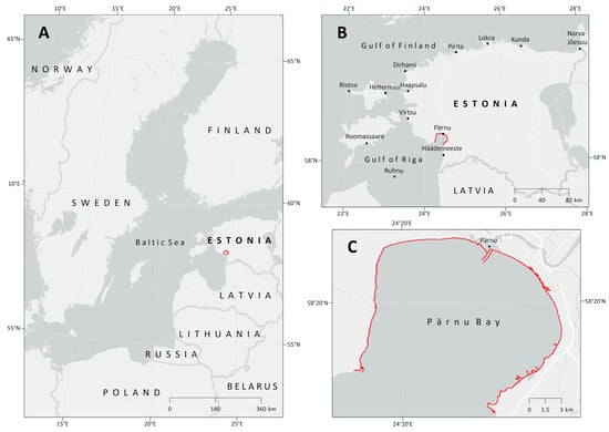
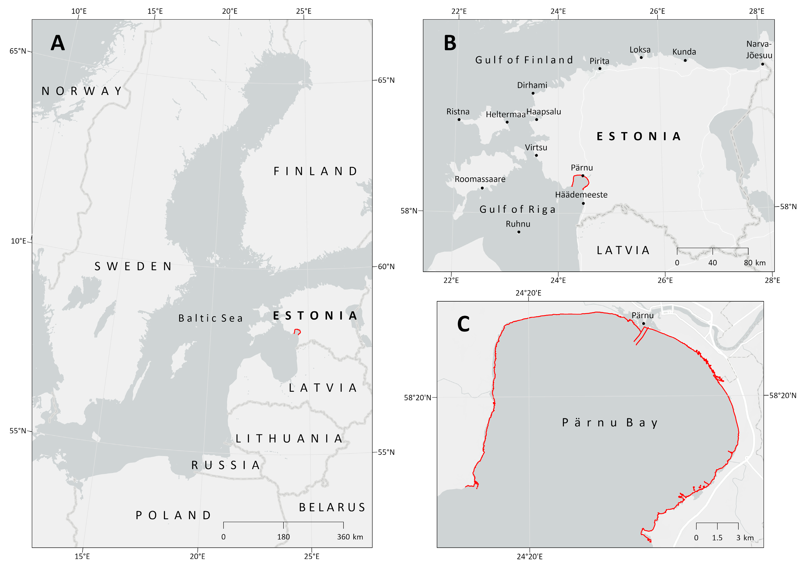
The study area is located along the coast of Pärnu Bay, on the southwestern coast of Estonia in the eastern Baltic Sea (Figure 1). The area is representative of the low-relief Baltic Sea shoreline.

Figure 1. Location of the study area (Pärnu Bay) on the Estonian coast in the eastern Baltic Sea. Panels show (A) the regional context of the Baltic Sea, (B) the locations of the tide gauge stations included in the study, and (C) the study area (red) along the coast of Pärnu Bay.

Pärnu Bay is a low-relief, semi-enclosed coastal area along the northeastern shore of the Gulf of Riga and is one of the lowest-lying and most morphodynamically active coastal regions in Estonia. It is a shallow and partially enclosed bay with an average water depth of less than 10 m. The coastal landscape is characterized by extensive sandy beaches, coastal lowlands, reed beds, wetlands, and sedimentary environments associated with the mouth of the Pärnu River. The area also contains Holocene beach ridges and marine terraces that reflect former shoreline positions and changes in relative sea level. Studies on Holocene shoreline development have shown that the Pärnu region has been sensitive to both sea-level fluctuations and sediment redistribution processes [33]. Similar shoreline changes have also been documented in other low-lying coastal regions of Estonia [34].

Long-term TG records indicate substantial intra-annual and interannual sea-level variability in the region with an annual range of approximately 100–200 cm (typically 120–180 cm) [9]. Such variability must be considered when interpreting shorelines extracted from remote sensing data. Wave action and wind-induced sea-level rise can temporarily shift the land–water boundary, particularly along gently sloping sandy beaches, estuarine environments, and deltaic environments. Given that long-term sea-level variability in the region typically reaches 120–180 cm, storm surges and wind-induced sea-level rise may result in horizontal shoreline displacements of several tens of meters in low-relief coastal areas. As a result, satellite-derived shorelines may vary considerably depending on the sea-level conditions at the time of image acquisition, thereby increasing differences among shoreline determination methods.

3. Data and Methods

The objective of this study is to compare shoreline determination methods based on different geospatial data sources by analyzing the horizontal differences between the shoreline delineated from a LiDAR-derived DTM using the observed sea level and instantaneous shorelines extracted from Sentinel-1 SAR and Sentinel-2 multispectral imagery. Horizontal displacement was defined as the planimetric distance between the shoreline products being compared. For the satellite analysis, horizontal differences were quantified between the satellite-derived shorelines and the corresponding temporally matched LiDAR-derived shorelines.

The analysis was based on four complementary datasets: (i) sea-level observations from TG stations from 2015 to 2025, (ii) a LiDAR-derived Digital Terrain Model (DTM), (iii) Sentinel-1 SAR imagery, and (iv) Sentinel-2 multispectral imagery. All datasets were transformed into the common national horizontal and vertical reference system (L-EST97/EH2000) to ensure positional consistency and comparability throughout the analysis.

The analytical workflow consisted of five main stages. First, long-term TG observations from the Estonian national monitoring network were analyzed to characterize sea-level variability along the Estonian coast. Simultaneously, observations from the Pärnu and Häädemeeste TGs were used to determine the mean TG sea level corresponding to the Sentinel-1 and Sentinel-2 satellite overpass times. Second, the land–water boundary was extracted from Sentinel-1 and Sentinel-2 observations acquired between 2015 and 2025. Third, LiDAR-derived shorelines were generated from the LiDAR-derived DTM acquired in 2021 using the Pärnu and Häädemeeste mean sea level at the satellite overpass time for each acquisition. Fourth, horizontal differences between the satellite-derived and temporally matched LiDAR-derived shorelines were quantified. Finally, satellite-derived shorelines were validated using GNSS measurements.

3.1. Tide Gauge Data

Sea-level data were obtained from automatic TG stations operated by the Estonian Environment Agency and equipped with pressure sensors. The dataset covers the period from 1 January 2015 to 31 December 2025, with instantaneous sea-level observations recorded at hourly intervals.

To characterize the regional hydrodynamic setting, long-term observations from 13 stations of the national TG network (Figure 1) were first compiled. Statistical metrics, including mean daily minimum, maximum, and MSL within the EH2000 vertical datum, were calculated separately for each station in order to place the sea-level dynamics of Pärnu Bay within the broader context of the Estonian shoreline. The main shoreline comparison focused on the Pärnu Bay region, where sea levels corresponding to the Sentinel-1 and Sentinel-2 overpass times were obtained from the Pärnu and Häädemeeste TGs. For each satellite acquisition, the arithmetic mean of the simultaneous observations from the two TGs was calculated and used as the elevation level for generating the corresponding temporally matched LiDAR-derived shoreline. Daily MSL values were retained as supplementary hydrodynamic information for comparison with the overpass-time sea levels.

3.2. Sentinel-1 SAR Data

Sentinel-1 SAR data were used to distinguish the land–water boundary at the time of image acquisition. The main processing steps applied to the Sentinel-1 data are presented in Figure 2.

Figure 2. Sentinel-1 SAR data processing steps.

The analysis utilized Ground Range Detected (GRD) products acquired in Interferometric Wide (IW) mode, with a spatial resolution of approximately 10 × 10 m. Classification was based on VH polarization, which is more sensitive to backscatter variations caused by surface roughness, facilitating discrimination between smooth water and rougher terrestrial surfaces. The analysis covered the period 2015–2025 and included only observations acquired during ice- and snow-free conditions to minimize their influence on the radar signal and ensure reliable water detection.

The discrimination of land and water surfaces was performed within the Copernicus Data Space Ecosystem environment [35] using an Evalscript-based processing workflow. The script converted linear VH backscatter values to decibels (dB) through a logarithmic transformation, providing a consistent signal scale across scenes and enabling more stable threshold-based classification.

Classification was based on a fixed empirical threshold of −18.0 dB, which was determined during a preliminary analysis of Sentinel-1 imagery acquired over representative Estonian coastal areas. Several candidate threshold values were evaluated, and −18.0 dB provided the most reliable separation between land and water based on visual assessment of the resulting shoreline classifications. Preliminary sensitivity testing using VH backscatter thresholds between −15 and −22 dB showed only minor differences in the extracted shoreline position. Therefore, the −18 dB threshold was retained for the final analysis. Pixels with values below the threshold were classified as water, whereas pixels with higher values were classified as land. The selected threshold is therefore regarded as a site-specific value for low-relief Estonian coastal environments and should not be directly applied to coastal regions with different vegetation structure, surface roughness, or radar backscatter characteristics without local calibration.

Areas containing missing data (dataMask = 0), which typically occur near image edges were classified as land to prevent the creation of artificial water bodies in the analysis. The resulting binary raster assigned a value of 255 to water and 0 to land. This raster was subsequently exported and converted into a line feature in ArcGIS Pro 3.6.2 (Esri, Redlands, CA, USA), representing the land–water boundary at the time of satellite overpass.

3.3. Sentinel-2 Multispectral Data

Sentinel-2 multispectral data acquired during the period 2015–2025 were used for the classification-based discrimination of land and water surfaces at the time of image acquisition. As with the Sentinel-1 analysis, only observations acquired during ice- and snow-free conditions were included to minimize seasonal effects and ensure reliable water detection. The main classification and processing steps applied to the Sentinel-2 data are presented in Figure 3.

Figure 3. Sentinel-2 multispectral data processing steps.

The analysis utilized atmospherically corrected Level-2A products, providing spectral bands and the Scene Classification Layer (SCL) for land-cover classification. The nominal revisit time of a single Sentinel-2 satellite is approximately 10 days. The Sentinel-2 data used in this study have a spatial resolution of 10 × 10 m.

Classification was performed within the Copernicus Data Space Ecosystem environment [35] using an Evalscript-based processing workflow. To discriminate between land and water surfaces, the Normalized Difference Water Index (NDWI) was calculated for each pixel using the green (B03) and near-infrared (B08) spectral bands. In addition, the Normalized Difference Vegetation Index (NDVI) was calculated using the red (B04) and near-infrared (B08) spectral bands to reduce false-positive classifications associated with vegetated surfaces.

Water classification was based on a combined decision-rule approach. A pixel was classified as water when the SCL identified it as class 6 (water), the NDWI value exceeded a threshold of 0.05, and the NDVI value remained below 0.2. This multi-criteria approach improves the discrimination of water from dark soils, shadows, and moist areas that may artificially increase NDWI values.

In addition, cloud shadows and clouds were excluded from the classification using Scene Classification Layer (SCL) classes 3 (cloud shadow), 8, and 9 (clouds). This step reduced the influence of atmospheric artefacts and improved the reliability of water classification. Areas at the edges of the imagery where the dataMask value was 0 were excluded from the analysis.

The resulting output was a binary raster in which a value of 255 represented water and a value of 0 represented land. The raster was exported and subsequently converted into a line feature in ArcGIS Pro, representing the land–water boundary at the time of satellite overpass.

All Sentinel-1 and Sentinel-2 images were processed using an identical workflow to ensure temporally consistent and reproducible shoreline extraction. The final comparison dataset was established by applying a set of acquisition-selection criteria. Only common Sentinel-1 and Sentinel-2 acquisition dates were retained, and these were further filtered to include only cloud-free, ice-free observations acquired under sufficiently calm sea-state conditions, and sea levels above 0.12 m, as lower sea levels did not permit reliable extraction of the LiDAR-derived shoreline from the DTM using the adopted methodology. Consequently, the final dataset represents selected common acquisition dates satisfying all methodological criteria rather than a temporally continuous annual sampling.

The extracted satellite-derived shorelines were subsequently compared with the corresponding LiDAR-derived shorelines generated as described in Section 3.4. Horizontal differences between the satellite-derived and temporally matched LiDAR-derived shorelines were quantified using the ArcGIS Pro Near tool (nearest-point distance method). In this method, points were generated at 5 m intervals along the satellite-derived shoreline. For each point, the Near tool in ArcGIS Pro identified the closest location on the corresponding LiDAR-derived shoreline and calculated the shortest Euclidean distance between the two. This unsigned shortest Euclidean distance was taken as the magnitude of the shoreline difference at the corresponding location. It should be noted that the nearest-point method does not independently determine whether the satellite-derived shoreline is displaced landward or seaward relative to the LiDAR-derived shoreline; this limitation is particularly relevant in geometrically complex, reed-dominated, and estuarine shoreline sections, where the direction of the shortest distance may deviate from the local shore-normal direction.

Based on these nearest-point distances, summary statistics were calculated, comprising both descriptive measures (mean, standard deviation, minimum, maximum, and median) and accuracy metrics (mean absolute error (MAE), root mean square error (RMSE), and the 90th percentile (P90)). Because the nearest-point distances are inherently unsigned and non-negative, the MAE is numerically equivalent to the mean nearest-point distance. In contrast, RMSE assigns proportionally greater weight to larger deviations, rendering it more sensitive than MAE to the influence of localized outliers, such as those arising from vegetation-obscured or morphologically complex shoreline segments.

In addition, all individual nearest-point distances from the temporally matched acquisitions were pooled separately for Sentinel-1 and Sentinel-2. The pooled distance distributions were summarized using percentage histograms, and corresponding pooled statistics (median, MAE, RMSE, P90, and maximum) were calculated to characterize the overall agreement between each satellite-derived shoreline product and the LiDAR-derived reference across all analyzed acquisitions.

3.4. LiDAR Data and LiDAR-Derived Shoreline

The LiDAR data used in this study were obtained from routine airborne laser scanning surveys conducted every four years by the Estonian Land and Spatial Development Board. Three airborne LiDAR campaigns have been conducted for the study area (2012, 2017, and 2021); however, the 2021 dataset was used in this study owing to its higher point density (2.1 points/m²) compared with the earlier surveys (0.45 points/m²). The 2021 point cloud was used to generate a DTM providing a detailed representation of topographic variability in low-relief coastal environments. The vertical accuracy of the dataset is between 0.03 and 0.07 m (standard deviation), as determined from RTK GNSS control measurements following the quality assessment procedures of the Estonian Land and Spatial Development Board [36].

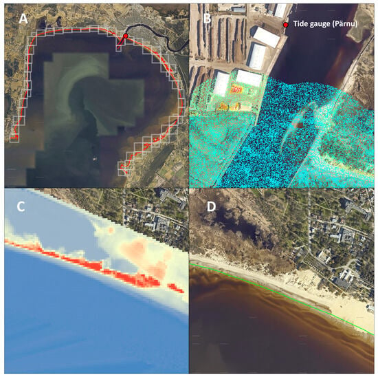
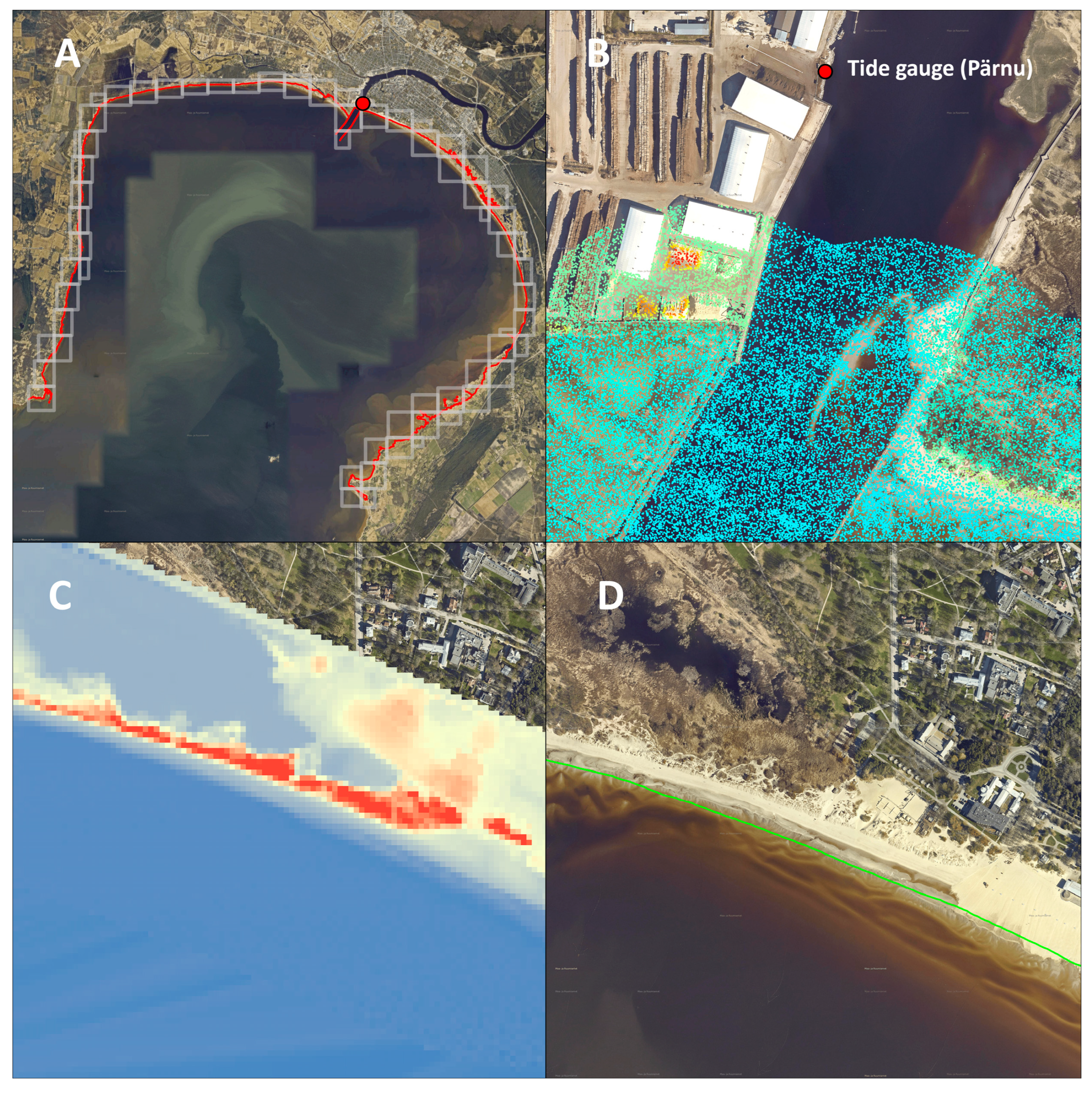
The LiDAR dataset was organized into 1 × 1 km map sheet tiles (Figure 4A). The DTM was generated using pre-classified points belonging to ASPRS classes 2 (ground) and 9 (water) (Figure 4B). The pre-classified dataset distinguishes terrestrial and water areas according to the national LiDAR classification scheme, resulting in all seaward areas being classified as water, although some points may in fact originate from the seabed. To minimize the influence of such artefacts, automated filtering procedures were combined with visual quality control. The DTM was interpolated to a spatial resolution of 1 m (Figure 4C).

Figure 4. Workflow for generating LiDAR-derived shorelines. Panels show (A) the LiDAR coverage area (grey) and the official shoreline from the Estonian Topographic Database (ETAK) (red), (B) the airborne LiDAR point cloud colored by elevation (blue to red indicating increasing elevation) and the location of the Pärnu tide gauge, (C) the LiDAR-derived digital terrain model (DTM) colored by elevation (blue to red indicating increasing elevation), and (D) an example of a LiDAR-derived shoreline (green) extracted from the DTM using the mean Pärnu–Häädemeeste tide gauge sea level at the satellite overpass time (0.25 m). Basemap: Estonian Land and Spatial Development Board orthophoto.

The shoreline contained in the Estonian Topographic Database (ETAK) [37], maintained by the Estonian Land and Spatial Development Board, was used to define the coastal study area and the 50 m landward buffer applied in the inter-epoch comparison of LiDAR-derived DTMs. Although the official shoreline was not used as the primary reference for the comparison between satellite-derived and LiDAR-derived shorelines, it provided a consistent spatial framework for the analysis.

To derive LiDAR-based shorelines for comparison with the satellite-derived shoreline products, elevation contours were generated separately for each Sentinel-1 and Sentinel-2 acquisition using the mean sea level observed at the Pärnu and Häädemeeste TGs at the satellite overpass time. For each acquisition, the arithmetic mean of the simultaneous observations from the two TGs was used as the elevation level for extracting the corresponding LiDAR-derived shoreline from the 2021 DTM. Daily MSL values were retained for comparison with the overpass time sea levels and as supplementary hydrodynamic information. An example of a LiDAR-derived shoreline generated using this procedure is shown in Figure 4D.

The resulting shoreline geometries were topologically cleaned by removing short isolated segments and interpolation artefacts while preserving the original elevation definition. The extracted contours are hereafter referred to as LiDAR-derived shorelines.

A comparison between the DTMs was performed to evaluate the temporal representativeness of the LiDAR-derived DTM used for shoreline extraction. Additional comparisons were therefore carried out between DTMs generated from the LiDAR datasets acquired during the airborne laser scanning campaigns of 2012, 2017, and 2021. Elevation differences between 2012, 2017, and 2021 DTMs were calculated within a 50 m landward buffer to assess the consistency of terrain representation in the coastal zone. Raster differences were calculated for DTM2017–DTM2012 and DTM2021–DTM2017. To characterize inter-epoch elevation variability beyond the mean difference, minimum, maximum, mean, median, standard deviation, mean and median absolute differences, RMSE, and P90 of the absolute elevation differences were calculated. Mean and median values retain the sign of the elevation difference, whereas the absolute statistics characterize the magnitude of inter-epoch elevation differences independently of their direction. The resulting inter-epoch DTM difference statistics are summarized in Table 2.

Table 2. Descriptive statistics of inter-epoch DTM elevation differences (m) within the 50 m coastal buffer.

Statistic	DTM2017–DTM2012	DTM2021–DTM2017
Points (N)	2,896,678	2,899,997
Min	−3.51	−4.00
Max	3.50	2.17
Mean	0.07	0.04
Median	0.06	0.04
Absolute mean	0.15	0.12
Absolute median	0.10	0.07
Std. Dev.	0.20	0.20
RMSE	0.22	0.21
P90	0.32	0.25

These statistics demonstrate that the relatively small mean signed elevation differences do not fully characterize the spatial variability between the LiDAR epochs. Although the 2021 DTM provides the most accurate and spatially detailed LiDAR-derived elevation dataset available for this study, localized inter-epoch terrain differences remain relevant when it is used as a reference for Sentinel acquisitions from different years. The implications of this temporal terrain variability for the satellite–LiDAR shoreline comparison are considered further in the Discussion.

4. Results

4.1. Sea-Level Analysis

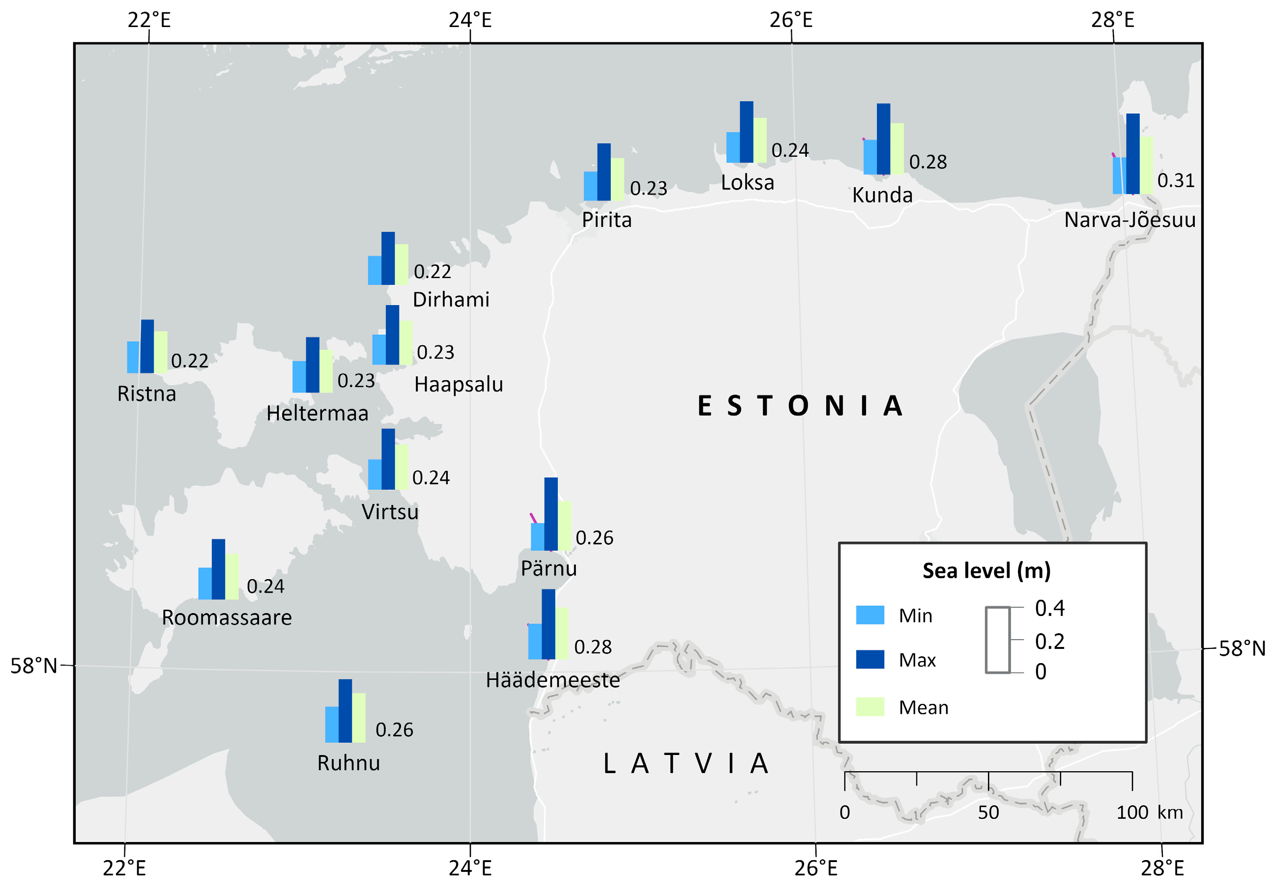
Table 3 and Figure 5 present the mean daily minimum, mean daily maximum, and MSL recorded at Estonian TG stations during 2015–2025, providing the hydrodynamic context for the shoreline analyses.

Table 3. Summary statistics of mean daily minimum, maximum, and mean sea levels (m) at Estonian tide gauge stations during 2015–2025.

Tide Gauge	Min SL	Max SL	MSL
Pärnu	0.15	0.39	0.26
Haapsalu	0.16	0.32	0.23
Heltermaa	0.17	0.30	0.23
Häädemeeste	0.19	0.38	0.28
Kunda	0.18	0.38	0.28
Loksa	0.16	0.33	0.24
Narva-Jõesuu	0.20	0.43	0.31
Pirita	0.16	0.30	0.23
Ristna	0.17	0.28	0.22
Roomassaare	0.17	0.32	0.24
Ruhnu	0.19	0.34	0.26
Virtsu	0.16	0.33	0.24
Dirhami	0.15	0.28	0.22
Mean	0.17	0.34	0.25

Figure 5. Mean daily minimum (light blue), maximum (dark blue), and mean (green) sea levels (m) at Estonian tide gauge stations during 2015–2025.

The mean daily maximum sea level varied among the analyzed TG stations, ranging from 0.28 to 0.43 m, whereas the mean daily minimum sea level ranged from 0.15 to 0.20 m. The overall MSL was 0.25 m, while noticeable regional differences were observed among the TGs.

Greater sea-level variability was observed at Narva-Jõesuu, Pärnu, and Kunda, as reflected by their higher mean daily maximum sea levels and MSL values (Table 3). These regional differences are likely associated with differences in local hydrodynamic setting, including coastal orientation and exposure to prevailing winds. In contrast, stations in western Estonia and on the islands (e.g., Ristna, Dirhami, and Heltermaa) exhibited lower MSL values and smaller daily variability.

Although the reported values represent average conditions, even relatively small vertical sea-level changes (e.g., 0.10–0.20 m) may result in substantial horizontal shoreline displacements along low-gradient coasts. These observations provide the hydrodynamic context for interpreting the shoreline analyses presented in the following sections.

4.2. Comparison of Sentinel-1-Derived and LiDAR-Derived Shorelines

To provide a more temporally consistent comparison between satellite-derived and elevation-based shoreline products, LiDAR-derived shorelines were re-extracted separately for each Sentinel-1 acquisition using the mean sea level observed at the Pärnu and Häädemeeste TGs at the satellite overpass time (Table 4). The horizontal differences between the Sentinel-1-derived and revised LiDAR-derived shorelines are presented in Table 5.

Table 4. Acquisition information and tide gauge sea levels (m) for the comparison between Sentinel-1-derived and LiDAR-derived shorelines.

Date	Satellite Overpass Time (UTC)	MSL in Pärnu TG at Overpass	MSL in Häädemeeste TG at Overpass	Difference Between TGs	Mean TG Sea Level at Overpass Used for LiDAR Shoreline Extraction	Daily MSL
7 August 2015	04:34	0.20	0.22	−0.02	0.21	0.22
16 November 2017	04:49	0.88	0.86	0.02	0.87	0.71
22 July 2018	04:34	0.14	0.18	−0.04	0.16	0.17
4 June 2019	04:42	0.22	0.18	0.04	0.20	0.19
27 September 2019	04:34	0.24	0.29	−0.05	0.27	0.23
1 December 2019	04:42	0.18	0.26	−0.08	0.22	0.24
22 May 2020	04:50	0.21	0.28	−0.07	0.25	0.27
14 June 2025	04:41	0.22	0.26	−0.05	0.24	0.26
25 July 2025	04:49	0.22	0.25	−0.03	0.24	0.22
14 August 2025	04:34	0.28	0.32	−0.05	0.30	0.30
18 October 2025	04:42	0.18	0.26	−0.09	0.22	0.29

Table 5. Horizontal shoreline differences (m) for the comparison between Sentinel-1-derived and LiDAR-derived shorelines.

Date	Comparison Points (N)	Min	Max	Mean	Std. Dev.	Median	MAE	RMSE	P90
7 August 2015	16,418	0.0	239.5	39.9	39.7	27.2	39.9	56.3	95.9
16 November 2017	15,279	0.0	436.3	76.8	84.0	47.0	76.8	113.8	201.3
22 July 2018	17,524	0.0	348.8	70.1	64.3	51.5	70.1	95.1	161.9
4 June 2019	16,826	0.0	193.6	41.6	41.0	27.1	41.6	58.4	104.2
27 September 2019	16,730	0.0	323.4	42.3	47.8	28.2	42.3	72.3	153.2
1 December 2019	13,557	0.0	242.2	39.9	36.7	28.2	39.9	54.2	91.8
22 May 2020	15,270	0.0	235.8	40.2	41.7	25.7	40.2	58.0	98.9
14 June 2025	16,702	0.0	219.1	39.3	37.5	27.6	39.3	54.4	89.8
25 July 2025	16,763	0.0	196.5	33.9	30.7	25.4	33.9	45.7	74.5
14 August 2025	15,613	0.0	244.1	42.3	37.1	31.8	42.3	56.2	94.4
18 October 2025	16,730	0.0	325.8	44.4	47.1	29.7	44.4	64.7	102.0
Mean across acquisitions *	16,128.4	0.0	273.2	46.4	46.1	31.8	46.4	66.3	115.3

* The final row represents the unweighted arithmetic mean of the acquisition-level summary statistics. It does not represent pooled statistics across all comparison points. Pooled nearest-point distance statistics are presented separately in Figure 6.

Although the magnitude of the differences varied between acquisition dates, no consistent relationship was observed between sea level and shoreline agreement. The largest spatial differences occurred primarily in low-relief coastal areas, reed beds, and estuarine environments, where small vertical changes in sea level produce substantial horizontal shoreline displacements. Overall, the results indicate that Sentinel-1-derived shorelines exhibit substantial differences relative to the LiDAR-derived shorelines even when both shoreline products were compared using common acquisition dates and LiDAR-derived shorelines extracted using the mean Pärnu–Häädemeeste TG sea level at the satellite overpass time.

4.3. Comparison of Sentinel-2-Derived and LiDAR-Derived Shorelines

The same revised comparison procedure was applied to Sentinel-2 (Table 6 and Table 7).

Table 6. Acquisition information and tide gauge sea levels (m) for the comparison between Sentinel-2-derived and LiDAR-derived shorelines.

Date	Satellite Overpass Time (UTC)	MSL in Pärnu TG at Overpass	MSL in Häädemeeste TG at Overpass	Difference Between TGs	Mean TG Sea Level at Overpass Used for LiDAR Shoreline Extraction	Daily MSL
7 August 2015	09:50	0.23	0.24	−0.01	0.23	0.22
16 November 2017	09:42	0.72	0.69	0.03	0.71	0.71
22 July 2018	09:50	0.13	0.18	−0.05	0.15	0.17
4 June 2019	09:40	0.22	0.23	−0.01	0.22	0.19
27 September 2019	09:40	0.27	0.32	−0.05	0.29	0.23
1 December 2019	09:43	0.15	0.21	−0.06	0.18	0.24
22 May 2020	09:50	0.25	0.32	−0.07	0.28	0.27
14 June 2025	09:40	0.27	0.32	−0.05	0.29	0.26
25 July 2025	09:50	0.26	0.29	−0.03	0.27	0.22
14 August 2025	09:50	0.29	0.34	−0.05	0.31	0.30
18 October 2025	09:50	0.20	0.27	−0.07	0.24	0.29

Table 7. Horizontal shoreline differences (m) for the comparison between Sentinel-2-derived and LiDAR-derived shorelines.

Date	Comparison Points (N)	Min	Max	Mean	Std. Dev.	Median	MAE	RMSE	P90
7 August 2015	11,639	0.0	225.2	33.0	30.2	24.2	33.0	44.7	69.9
16 November 2017	11,632	0.0	586.6	71.2	93.4	33.0	71.2	117.5	191.2
22 July 2018	11,730	0.0	363.1	67.3	87.2	24.8	67.3	110.1	245.5
4 June 2019	11,460	0.0	338.5	17.8	20.9	13.2	17.8	27.4	34.8
27 September 2019	11,863	0.0	339.5	30.5	28.5	23.9	30.5	41.7	62.6
1 December 2019	11,848	0.0	377.0	32.2	50.6	15.0	32.2	60.0	87.4
22 May 2020	11,476	0.0	153.2	17.2	18.9	12.0	17.2	25.6	34.2
14 June 2025	10,885	0.0	409.1	58.6	87.0	25.0	58.6	104.8	199.2
25 July 2025	11,598	0.0	244.6	45.6	48.5	26.2	45.6	66.5	120.7
14 August 2025	11,211	0.0	238.0	46.0	48.9	27.3	46.0	67.1	121.4
18 October 2025	12,096	0.0	194.2	31.3	30.3	20.9	31.3	43.6	72.3
Mean across acquisitions	11,585.3	0.0	315.4	41.0	49.5	22.3	41.0	64.5	112.7

Compared with Sentinel-1, Sentinel-2 generally showed smaller mean horizontal differences for most acquisition dates, indicating closer agreement with the LiDAR-derived shoreline under the analyzed conditions. Nevertheless, localized large differences remained evident in some acquisition dates, particularly within reed beds and estuarine environments, reflecting the influence of local morphology on shoreline position.

Overall, the temporally matched comparison demonstrated that Sentinel-2-derived shorelines generally corresponded more closely to the LiDAR-derived shorelines than Sentinel-1-derived shorelines under the analyzed conditions. Nevertheless, differences remained between the shoreline products, including localized large differences in some acquisition dates. Consequently, Sentinel-2 data showed potential for mapping the instantaneous land–water boundary under the cloud-free conditions evaluated in this study, although this interpretation is specific to the environmental and methodological conditions examined.

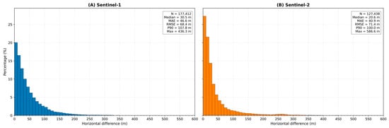
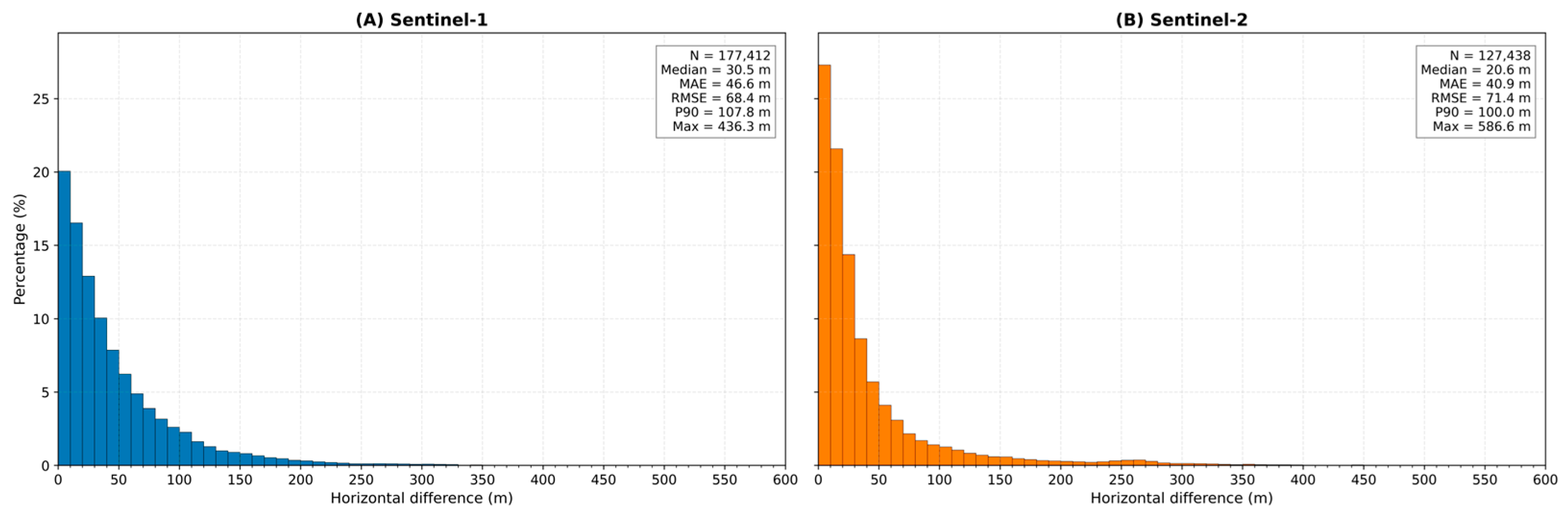
The distribution of horizontal differences for all temporally matched shoreline comparisons is presented in Figure 6. Approximately 77.6% and 67.4% of the shoreline differences were smaller than 50 m for Sentinel-2 and Sentinel-1, respectively. The corresponding P90 values were 100.0 m for Sentinel-2 and 107.8 m for Sentinel-1. The pooled distributions also showed median distances of 20.6 m for Sentinel-2 and 30.5 m for Sentinel-1, while the corresponding MAE values were 40.9 m and 46.6 m, respectively. These distributions indicate generally smaller typical shoreline differences for Sentinel-2, although its RMSE (71.4 m) and maximum distance (586.6 m) were higher than those of Sentinel-1 (68.4 m and 436.3 m, respectively), indicating the presence of localized large differences in the Sentinel-2 dataset.

Figure 6. Pooled distributions of unsigned nearest-point distances between temporally matched LiDAR-derived shorelines and the corresponding (A) Sentinel-1-derived and (B) Sentinel-2-derived shorelines across all analyzed acquisition dates.

4.4. Overall Comparison of Satellite-Derived Shorelines

To provide an overall comparison of the evaluated shoreline products, pooled distance statistics were calculated from all temporally matched nearest-point distances for Sentinel-1 and Sentinel-2 separately. These pooled statistics provide an overall quantitative characterization of shoreline agreement across all analyzed acquisition dates. The acquisition-level distance statistics and their unweighted arithmetic means are summarized in Table 5 and Table 7, whereas the pooled nearest-point distance distributions and corresponding pooled statistics across all acquisitions are presented in Figure 6.

The pooled statistics showed that Sentinel-2 had a lower median nearest-point distance (20.6 m vs. 30.5 m), lower MAE (40.9 m vs. 46.6 m), and lower P90 (100.0 m vs. 107.8 m) than Sentinel-1. However, the RMSE and maximum distance were higher for Sentinel-2, indicating that its distance distribution included localized large differences despite the generally lower typical separation.

These differences reflect not only the influence of hydrodynamic conditions but also the different physical measurement principles of radar and optical remote sensing, which represent different manifestations of the land–water boundary.

Overall, the results demonstrate substantial differences between the shoreline products derived from Sentinel-1 and Sentinel-2 even when based on temporally matched observations. Sentinel-2-derived shorelines generally showed lower median, MAE, and P90 values than Sentinel-1-derived shorelines, although the higher RMSE and maximum distance indicate that both datasets exhibited substantial spatial variability and localized large differences in the low-relief coastal environment. These findings indicate that radar- and optical-derived shorelines represent different physical manifestations of the land–water boundary and therefore should not be considered directly interchangeable.

5. Validation

The positional accuracy of shorelines derived from Sentinel-1 and Sentinel-2 imagery was assessed using a shoreline surveyed with RTK GNSS. The field survey followed the observed land–water boundary and provided a field-based shoreline surveyed during the same morning under changing water-level conditions.

5.1. Field Survey

RTK GNSS measurements were conducted in the Pärnu Bay region on 23 April 2026 between 05:30 and 12:00 UTC to coincide with Sentinel-1 (04:28 UTC) and Sentinel-2 (10:15 UTC) satellite overpasses on the same day. Coordinates were recorded in the Estonian national coordinate system (L-EST97) and referenced to the EH2000 vertical datum using real-time corrections from the ESTPOS network. The survey was performed using a South ALPS1 RTK GNSS receiver with a specified horizontal and vertical accuracy of 0.8 cm and 1.5 cm, respectively. The visually identifiable land–water boundary was surveyed by recording GNSS positions at approximately 60 m intervals, and the measured points were connected to generate the GNSS-derived shoreline. A total of 534 GNSS points were surveyed along approximately 21 km of coastline. The survey covered representative coastal environments, including sandy beaches, coastal lowlands, reed beds, and estuarine areas. Point spacing varied depending on shoreline accessibility and morphology. Measurements were carried out under moderate northerly winds (6–10 m/s). As the offshore wind generated only limited wave activity within the survey area, the land–water boundary was clearly identifiable throughout the survey.

During the survey, sea level ranged from +10 cm to −13 cm relative to the EH2000 vertical datum. In low-relief coastal environments, such variations may shift the shoreline horizontally by several tens of meters. Consequently, the GNSS-derived shoreline represents the observed land–water boundary along the surveyed coastline during the field survey rather than a single strictly instantaneous or elevation-defined shoreline.

The vertical quality of the GNSS measurements was assessed by comparing RTK GNSS-derived water-surface elevations with simultaneous observations from the Pärnu TG referenced to the EH2000 vertical datum. The mean difference between the RTK GNSS-derived water-surface elevations and the simultaneously observed Pärnu TG sea level was only 2 cm, confirming the reliability of the GNSS elevation measurements and indicating negligible systematic vertical bias during the survey. Sentinel-1-derived shorelines were validated 1) along the entire surveyed coastline (approximately 21 km), and 2) along the same approximately 7 km cloud-free shoreline section used for the Sentinel-2 validation. This additional comparison enabled a direct evaluation of the two satellite-derived shoreline products over an identical shoreline extent (Figure 7).

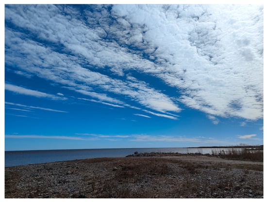
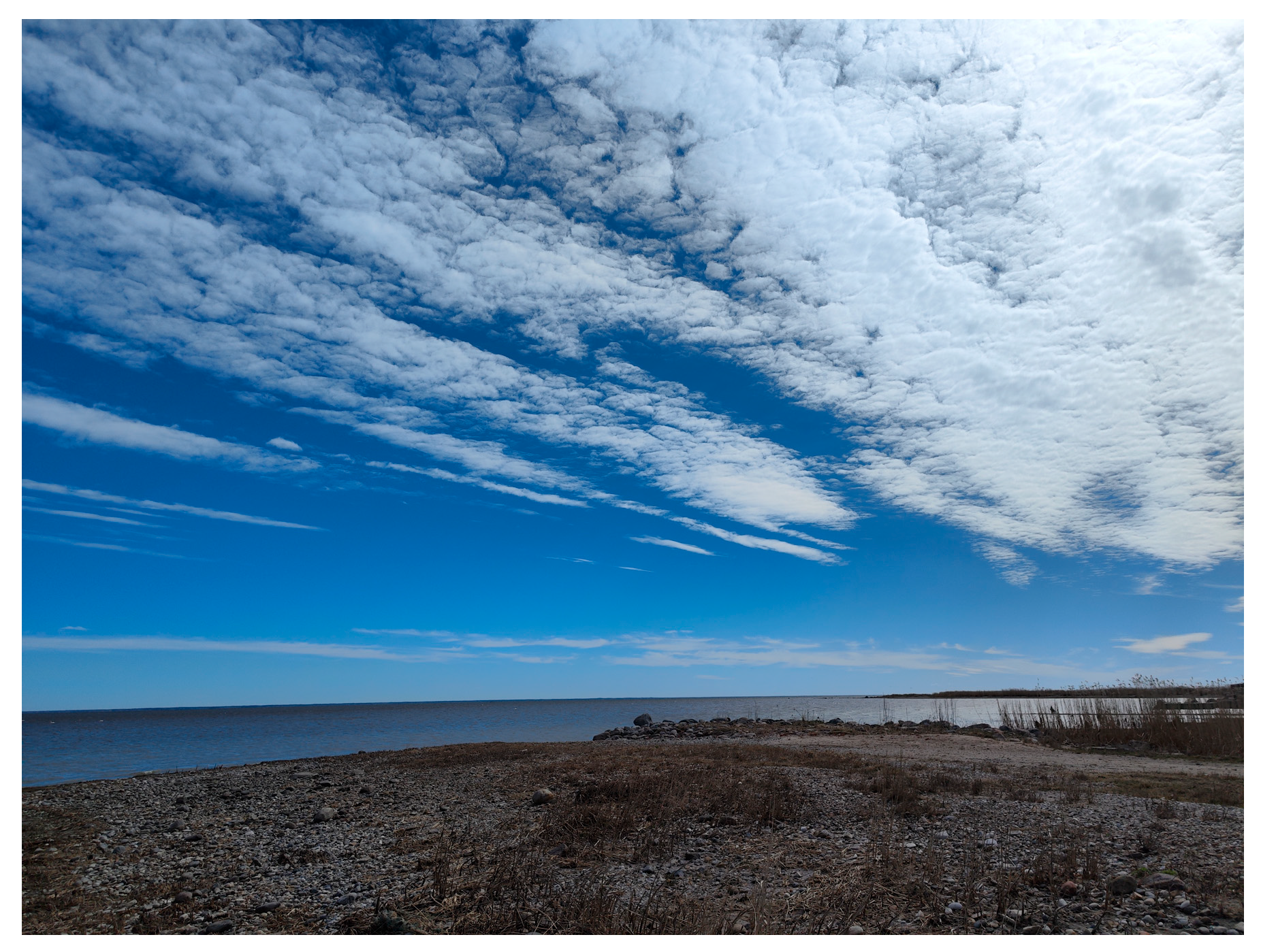
Figure 7. Cloud cover over Pärnu Bay during the Sentinel-2 overpass (23 April 2026, 10:15 UTC).

5.2. Satellite Shoreline Validation

Satellite-derived shorelines from Sentinel-1 and Sentinel-2 imagery were validated against the RTK GNSS-derived shoreline using the ArcGIS Pro Near tool. For each GNSS validation point, the shortest Euclidean distance to the satellite-derived shoreline was calculated and used as the magnitude of the shoreline difference. These distances are unsigned and therefore do not independently indicate whether the satellite-derived shoreline is located landward or seaward of the GNSS-derived shoreline.

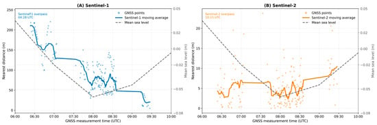
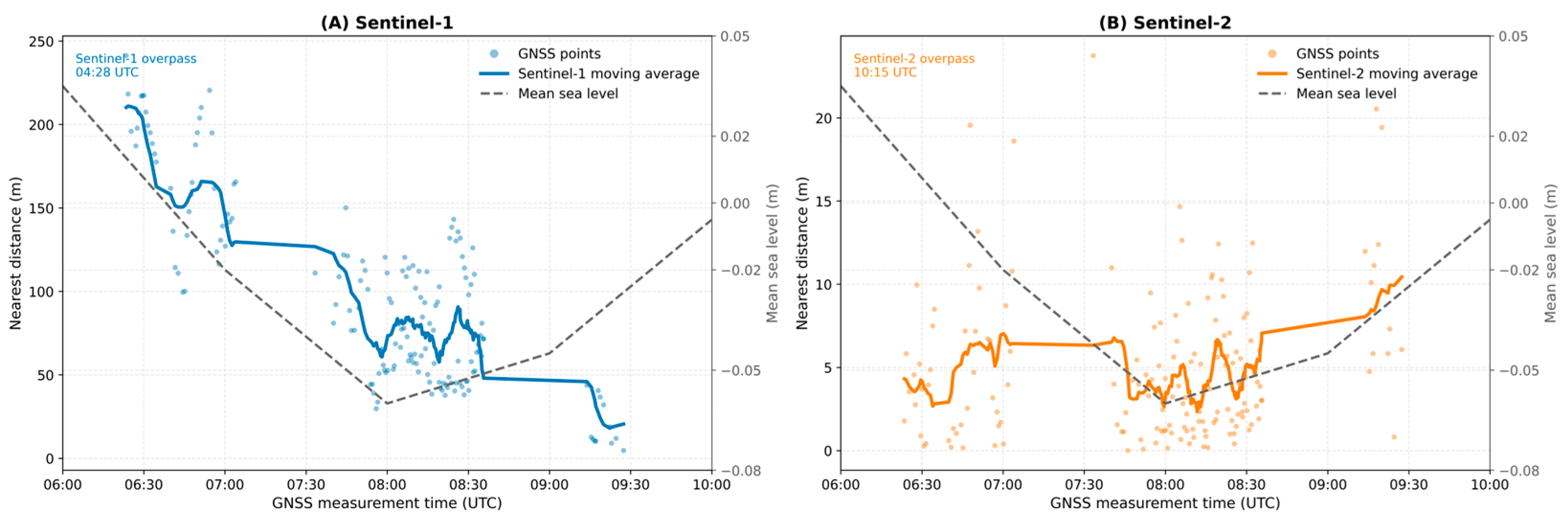
All GNSS observations were time-stamped during the field survey. To further evaluate the temporal behavior of the GNSS validation, an additional analysis was performed for the common 7 km validation section used for both Sentinel-1 and Sentinel-2. The nearest distances between the GNSS-derived shoreline and the satellite-derived shorelines were analyzed as a function of GNSS measurement time.

For Sentinel-2, the validation was limited to approximately 7 km of shoreline where cloud-free imagery allowed reliable land–water boundary extraction (Figure 7). To enable a direct comparison between the two satellite products, Sentinel-1 was validated both along the entire surveyed coastline (21 km) and along the same 7 km cloud-free shoreline section. In addition to the statistical analysis of horizontal differences, their spatial distribution was examined to identify coastal sections exhibiting systematically larger or smaller nearest-point distances between the satellite-derived and GNSS-derived shorelines.

One limitation of optical satellite imagery is cloud cover, which reduces the length of shoreline available for validation and may introduce spatial gaps in the extracted shoreline. In this study, cloud and cloud-shadow pixels were excluded using the Sentinel-2 Scene Classification Layer (SCL), thereby restricting the validation to cloud-free shoreline sections. Future studies may further benefit from incorporating additional cloud-free acquisitions or multi-temporal image combinations to increase shoreline coverage while maintaining reliable shoreline extraction.

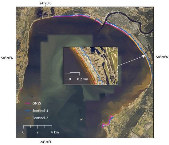
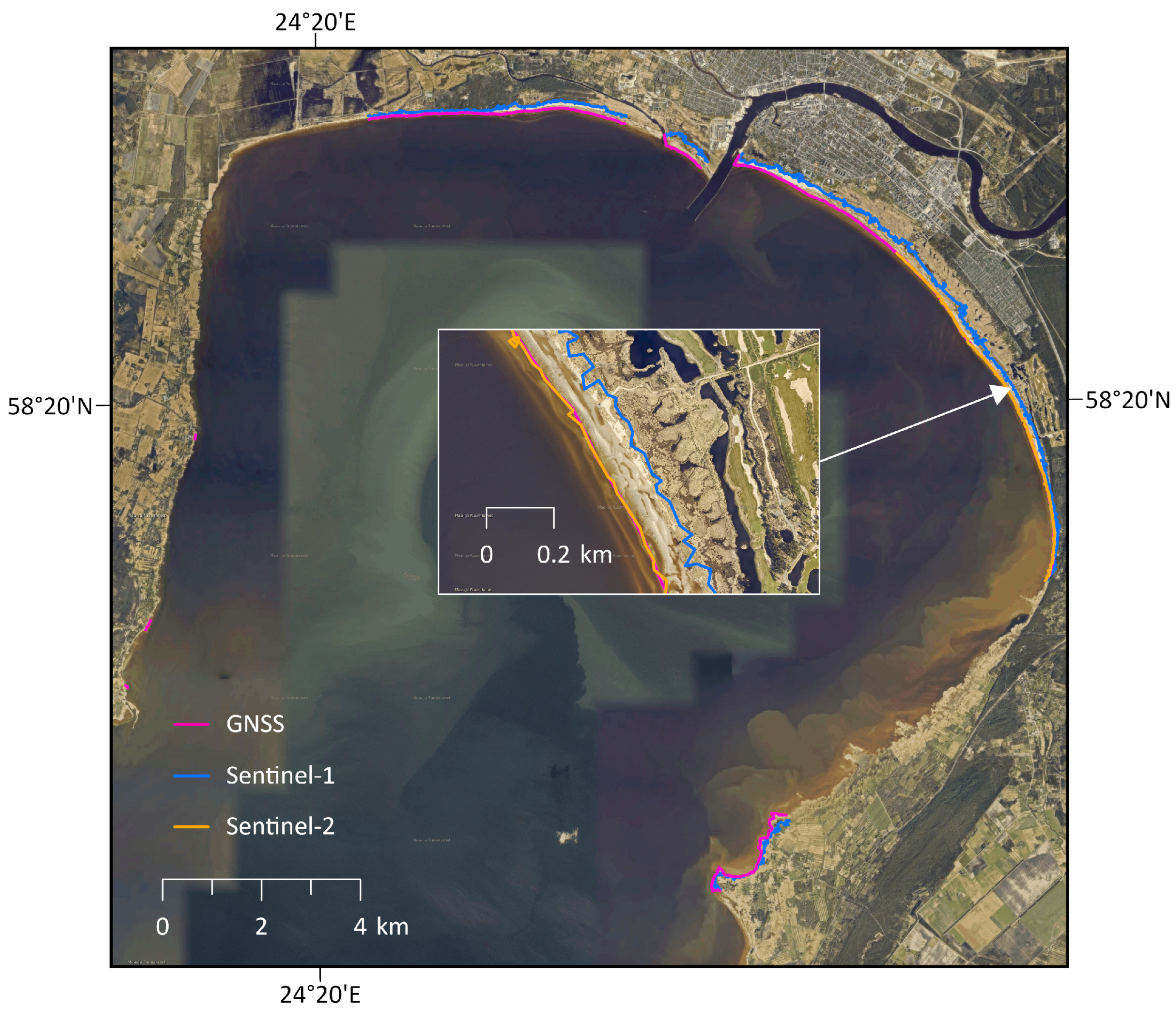
Figure 8 compares the GNSS-derived shoreline with the shorelines derived from Sentinel-1 and Sentinel-2 imagery, while Table 8 summarizes the corresponding horizontal differences.

Figure 8. Comparison of GNSS-, Sentinel-1-, and Sentinel-2-derived shorelines in Pärnu Bay (23 April 2026). Basemap: Estonian Land and Spatial Development Board orthophoto.

Table 8. Horizontal differences (m) between Sentinel-1-, Sentinel-2-, and GNSS-derived shorelines (23 April 2026).

Method	Shoreline Length (km)	Number of GNSS Points	Min	Max	Mean	Std. Dev.
Sentinel-1	21	534	0.1	338.2	129.9	73.5
Sentinel-1	7	166	3.3	338.2	134.9	69.8
Sentinel-2	7	166	0.0	49.5	6.0	6.4

For the common 7 km validation section, Figure 9 additionally shows the mean sea level derived from the Pärnu and Häädemeeste TG observations corresponding to the validation period. Sentinel-1 nearest distances exhibited greater temporal variability during the survey period, whereas Sentinel-2 nearest distances remained comparatively low and stable. These results provide additional insight into the temporal behavior of the GNSS validation during the field survey.

Figure 9. Temporal distribution of the nearest distances between the GNSS-derived shoreline, and (A) Sentinel-1-derived and (B) Sentinel-2-derived shorelines for the common 7 km validation section.

To enable a direct comparison between the two satellite-derived shoreline products, Sentinel-1 validation statistics were calculated both for the entire surveyed coastline (21 km) and for the same 7 km cloud-free shoreline section used for Sentinel-2. Restricting the Sentinel-1 validation to the common shoreline section resulted in only a small increase in the mean horizontal difference (129.9 m to 134.9 m), indicating that the substantially better agreement observed for Sentinel-2 cannot be explained solely by differences in the validated shoreline extent.

Within the common 7 km validation section, the Sentinel-2-derived shoreline closely matched the GNSS-derived shoreline, with a mean horizontal difference of 6.0 ± 6.4 m and a maximum difference of 49.5 m. Although the validation was limited to cloud-free shoreline sections, Sentinel-2 showed substantially better agreement with the GNSS-derived shoreline than Sentinel-1 under the prevailing survey conditions.

In contrast, the Sentinel-1-derived shoreline showed substantially larger deviations, with a mean horizontal difference of 134.9 ± 69.8 m and a maximum difference of 338.2 m. The largest discrepancies occurred in coastal lowlands, reed beds, and estuarine environments.

Overall, the validation demonstrates that Sentinel-2 imagery represented the instantaneous land–water boundary considerably more accurately than Sentinel-1 SAR imagery under the survey conditions. The reasons for these differences and their implications are discussed in Section 6.

6. Discussion

The results demonstrate that shoreline determination in low-relief coastal environments depends strongly on the data source, the applied shoreline concept, the vertical reference framework, and the timing of observations. The temporally matched comparison between satellite-derived and LiDAR-derived shoreline products showed that Sentinel-2 generally exhibited smaller horizontal differences than Sentinel-1 under common acquisition dates using LiDAR-derived shorelines extracted at the mean Pärnu–Häädemeeste TG sea level corresponding to the satellite overpass time. These findings demonstrate that the evaluated methods do not identify the same shoreline but rather represent different shoreline manifestations arising from sensor-specific remote-sensing sensitivities under particular hydrodynamic conditions.

The expanded inter-epoch DTM comparison showed relatively small mean signed elevation differences between the available LiDAR epochs; however, the standard deviation, RMSE, and P90 values indicate greater localized elevation variability than suggested by the mean values alone. Although the 2021 DTM represents the most accurate and spatially detailed LiDAR-derived elevation dataset available for this study, its use as a reference for Sentinel acquisitions from different years introduces uncertainty associated with local terrain changes. Localized erosion, accretion, vegetation-related surface changes, dredging, or anthropogenic modification between the LiDAR survey epochs and the Sentinel acquisition dates may therefore contribute to the observed Sentinel–LiDAR shoreline differences. This uncertainty is particularly relevant in the low-relief coastal environment of Pärnu Bay, where relatively small vertical elevation differences may translate into substantially larger horizontal shore-line-position differences. The magnitude of this horizontal uncertainty depends on the local coastal slope and therefore cannot be represented by a single study-area-wide horizontal uncertainty value.

Sentinel-1 and Sentinel-2 represent fundamentally different approaches to shoreline delineation. Sentinel-1 identifies the land–water boundary from radar backscatter and is largely independent of cloud cover and illumination conditions, whereas Sentinel-2 relies on optical reflectance and is therefore sensitive to surface moisture, vegetation, shadows, and sediment characteristics. Consequently, neither satellite-derived shoreline is referenced to a fixed vertical datum; instead, both represent the instantaneous land–water boundary observed by different remote sensing principles.

The comparison based on LiDAR-derived shorelines extracted using the mean Pärnu–Häädemeeste TG sea level at the satellite overpass time demonstrated that, although the horizontal differences varied between individual acquisition dates, the overall relationships between the evaluated shoreline products remained consistent. These findings indicate that the principal differences observed between LiDAR-, Sentinel-1-, and Sentinel-2-derived shorelines cannot be explained solely by differences in acquisition timing but also reflect the different shoreline concepts and physical measurement principles represented by the evaluated methods.

The GNSS validation highlights the importance of distinguishing between elevation-based and instantaneous shoreline representations. It should be emphasized that the GNSS survey represents a single-date validation conducted under specific hydrodynamic and environmental conditions. Consequently, the results should be interpreted as a field-based validation of the satellite-derived shoreline products under the environmental and changing sea-level conditions prevailing during the survey rather than as validation against a strictly instantaneous shoreline reference. The additional time-based analysis of the common 7 km validation section further illustrates the temporal behavior of the validation results within the temporal framework of the field survey. This interpretation is supported by the temporally matched comparison, which showed that Sentinel-2-derived shorelines generally corresponded more closely to the temporally matched LiDAR-derived shorelines than Sentinel-1-derived shorelines when evaluated using common acquisition dates and LiDAR-derived reference shorelines extracted at the mean Pärnu–Häädemeeste TG sea level corresponding to the satellite overpass time.

To enable a direct comparison between the two satellite-derived shoreline products, Sentinel-1 validation statistics were also calculated for the same 7 km cloud-free shoreline section used for Sentinel-2. Restricting the Sentinel-1 validation to the common shoreline section resulted in only a minor increase in the mean horizontal difference (from 129.9 m to 134.9 m), indicating that the substantially better agreement observed for Sentinel-2 cannot be explained solely by differences in the validated shoreline extent.

Under the prevailing survey conditions, Sentinel-2 represented the observed land–water boundary considerably more accurately than Sentinel-1, with a mean horizontal difference of 6.0 ± 6.4 m compared with 134.9 ± 69.8 m for Sentinel-1 over the same shoreline section. Together, these findings support the interpretation that the fundamentally different land–water boundary detection concepts employed by Sentinel-1 and Sentinel-2 lead to different shoreline representations and, consequently, different levels of shoreline delineation accuracy.

The contrasting validation results can be explained by both the environmental conditions during the field survey and the different physical measurement principles of the two satellite sensors. During the GNSS survey, sea level ranged from −0.13 to +0.10 m (mean 0.03 m), while wave activity remained limited. Under these conditions, Sentinel-2 optical imagery accurately delineated the instantaneous land–water boundary based on surface reflectance characteristics. In contrast, Sentinel-1 SAR imagery detects differences in radar backscatter, which is strongly influenced by vegetation structure and surface roughness. Consequently, reed beds and other rough vegetated surfaces may generate radar returns similar to those of dry land, causing water-covered areas to be classified as land and contributing to larger positional differences between the Sentinel-1-derived and reference shorelines in vegetated coastal sections.

The additional temporal analysis presented in Figure 9 further indicates that, within the common 7 km validation section, the smallest Sentinel-1 nearest distances occurred during the period of lower mean sea level derived from the simultaneous Pärnu and Häädemeeste TG observations. Under lower sea-level conditions, a wider sandy beach may be exposed, which may increase the spatial separation between the GNSS-derived instantaneous shoreline and the wet–dry transition zone detected by the SAR signal. This interpretation is consistent with previous studies indicating that SAR-derived shoreline position is influenced by sea level together with radar viewing geometry, coastal morphology, and the wet–dry sand transition in low-relief coastal environments [38].

TG observations further demonstrate that even relatively small variations in sea level may produce horizontal shoreline shifts of several tens of meters along low-relief coasts. Consequently, the observed horizontal differences should not be interpreted solely as measurement errors but also as a manifestation of the combined influence of sensor characteristics, sea-level variability, and coastal morphology.

The restriction of the satellite analysis to the ice-free season introduced only a minor bias. Comparison of the Pärnu TG record showed that the difference between the mean annual sea level and the MSL during the satellite observation period was approximately 3 cm. Even along the very gently sloping coast of Pärnu Bay, this difference is insufficient to explain the horizontal shoreline differences observed in this study. The results therefore indicate that the observed differences primarily reflect the characteristics of the applied sensors and shoreline extraction methods rather than seasonal sampling.

From a methodological perspective, the shoreline comparison was based on the nearest-point distance method. An additional limitation is that the nearest-point distances are unsigned and are not constrained to the local shore-normal direction. Therefore, they quantify the magnitude of shoreline separation but provide limited support for interpreting the direction of shoreline displacement, particularly along curved, reed-dominated, and estuarine shoreline sections. Although this approach is straightforward and widely applied, it does not account for local coastal slope. Consequently, identical vertical changes in sea level or local terrain elevation may produce markedly different horizontal shoreline displacements depending on local topography. Future studies should therefore integrate local coastal-slope information to quantify more explicitly how vertical sea-level variability and terrain-elevation uncertainty propagate into horizontal shoreline-position uncertainty.

A further methodological limitation is that the sensitivity of the Sentinel-2 shoreline extraction to the adopted NDWI (>0.05) and NDVI (<0.2) thresholds was not independently evaluated in this study. Although these thresholds were applied together with the SCL water classification, their potential influence on the extracted shoreline position remains a source of uncertainty.

The results further demonstrate that different shoreline determination methods provide complementary information for different scientific and operational applications. LiDAR combined with TG observations provides a suitable basis for delineating elevation-referenced shorelines because it is linked to a defined vertical reference framework. Sentinel-1 SAR imagery provides weather- and illumination-independent observations and may therefore complement shoreline monitoring where optical imagery is unavailable. Under the cloud-free conditions evaluated in this study, Sentinel-2 optical imagery showed closer agreement with the field-observed land–water boundary and therefore demonstrated potential for mapping the instantaneous shoreline.

Overall, the findings demonstrate that shorelines derived from different data sources represent different spatial and temporal characteristics of the coastal zone. Elevation-based methods define a shoreline referenced to a fixed vertical datum, whereas satellite observations capture the instantaneous position of the land–water boundary under prevailing environmental conditions. Integrating these complementary datasets provides a more comprehensive representation of shoreline position and variability, improving both scientific analyses and operational coastal management.

7. Conclusions

This study demonstrates that shoreline determination in low-relief coastal environments depends on the data source, the shoreline concept, the vertical reference framework, and the timing of data acquisition. Rather than identifying a single objectively defined shoreline, the evaluated methods represent different shoreline definitions linked to distinct temporal and vertical reference frameworks. Consequently, they serve different scientific and practical purposes.

The temporally matched comparison demonstrated that Sentinel-2-derived shorelines generally corresponded more closely to the temporally matched LiDAR-derived shorelines than Sentinel-1-derived shorelines under common acquisition dates when the LiDAR-derived reference shorelines were extracted using the mean Pärnu–Häädemeeste TG sea level at the corresponding satellite overpass time. In contrast, satellite-derived shorelines represent the instantaneous land–water boundary and are therefore strongly influenced by sea-level conditions and environmental characteristics at the time of image acquisition. The field validation, including the comparison over the same 7 km shoreline section for both satellite datasets, further supported the interpretation that Sentinel-2 more closely represented the instantaneous land–water boundary under the cloud-free survey conditions investigated in this study.

An important implication of this study is that even small variations in sea level may produce horizontal shoreline displacements of several tens of meters along low-relief coasts. Consequently, shoreline position should always be interpreted in relation to the applied vertical reference framework, coastal morphology, and hydrodynamic conditions rather than as a fixed geometric boundary.

From a practical perspective, under the conditions and methodological framework evaluated in this study, LiDAR combined with TG observations provides a suitable approach for delineating an elevation-based reference shoreline, whereas Sentinel-1 and Sentinel-2 provide complementary information for operational shoreline monitoring. Sentinel-1 offers the potential for weather-independent shoreline observations, while Sentinel-2 showed potential for mapping the instantaneous land–water boundary under the cloud-free conditions examined in this study. These interpretations should be considered in light of the study limitations, including the single-date GNSS validation, the approximately 7 km cloud-free Sentinel-2 validation section, the use of an empirical Sentinel-1 backscatter threshold, the untested sensitivity of the Sentinel-2 classification thresholds, the use of unsigned nearest-point distances, and the uncertainty associated with using the 2021 DTM as an elevation reference for Sentinel acquisitions from different years.

Overall, the study demonstrates that shoreline datasets derived from Sentinel-1, Sentinel-2, and LiDAR combined with sea-level observations should not be considered directly interchangeable. Because these approaches delineate the land–water boundary using different detection principles, the differences between them primarily indicate the methods’ sensitivity and reliability under specific hydrodynamic conditions, which in turn reflect differences in positional accuracy. Integrating elevation-based and satellite-derived shoreline products provides complementary information on shoreline position and variability, and may provide a more robust basis for shoreline mapping and coastal monitoring in low-relief coastal environments when the methodological limitations and environmental conditions associated with each data source are explicitly considered.

References

- Boak, E.H.; Turner, I.L. Shoreline definition and detection: A review. J. Coast. Res. 2005, 21, 688–703. [Google Scholar] [CrossRef] [Scilit]
- Pajak, M.J.; Leatherman, S. The high water line as shoreline indicator. J. Coast. Res. 2002, 18, 329–337. [Google Scholar]
- Hapke, C.J.; Himmelstoss, E.A.; Kratzmann, M.G.; List, J.H.; Thieler, E.R. National Assessment of Shoreline Change: Historical Shoreline Change Along the New England and Mid-Atlantic Coasts; U.S. Geological Survey Open-File Report 2010–1118; U.S. Geological Survey: Reston, VA, USA, 2011; p. 57. Available online: https://pubs.usgs.gov/of/2010/1118/ (accessed on 12 April 2026).
- Stockdon, H.F.; Sallenger, A.H.; List, J.H.; Holman, R.A. Estimation of shoreline position and change using airborne topographic lidar data. J. Coast. Res. 2002, 18, 502–513. [Google Scholar]
- Toure, S.; Diop, O.; Kpalma, K.; Maiga, A.S. Shoreline detection using optical remote sensing: A review. ISPRS Int. J. Geo-Inf. 2019, 8, 75. [Google Scholar] [CrossRef] [Scilit]
- Leppäranta, M.; Myrberg, K. Physical Oceanography of the Baltic Sea; Springer: Berlin, Germany, 2009. [Google Scholar]
- Suursaar, Ü.; Kullas, T.; Otsmann, M.; Kõuts, T. Extreme sea level events in the coastal waters of western Estonia. J. Sea Res. 2003, 49, 295–303. [Google Scholar] [CrossRef] [Scilit]
- Suursaar, Ü.; Kullas, T.; Szava-Kovats, R.; Brebbia, C.A.; Jovanovic, N.; Tiezzi, E. Wind and wave storms, storm surges and sea level rise along the Estonian coast of the Baltic Sea. In Management of Natural Resources, Sustainable Development and Ecological Hazards II; WIT Press: Billerica, MA, USA, 2010; Volume 127, pp. 149–160. [Google Scholar] [CrossRef] [Scilit]
- Suursaar, Ü.; Sooäär, J. Decadal variations in mean and extreme sea level values along the Estonian coast of the Baltic Sea. Tellus A 2007, 59, 249–260. [Google Scholar] [CrossRef] [Scilit]
- Johansson, M.M.; Boman, H.; Kahma, K.K.; Launiainen, J. Trends in sea level variability in the Baltic Sea. Boreal Environ. Res. 2001, 6, 159–179. [Google Scholar]
- Myrberg, K.; Korpinen, S.; Uusitalo, L. Physical oceanography sets the scene for the Marine Strategy Framework Directive implementation in the Baltic Sea. Mar. Policy 2019, 107, 10391. [Google Scholar] [CrossRef] [Scilit]
- Soomere, T. Numerical simulations of wave climate in the Baltic Sea: A review. Oceanologia 2023, 65, 117–140. [Google Scholar] [CrossRef] [Scilit]
- Rantanen, M.; van den Broek, D.; Cornér, J.; Sinclair, V.A.; Johansson, M.M.; Särkkä, J.; Laurila, T.K.; Jylhä, K. The impact of serial cyclone clustering on extremely high sea levels in the Baltic Sea. Geophys. Res. Lett. 2024, 51, e2023GL107203. [Google Scholar] [CrossRef] [Scilit]
- Vestøl, O.; Ågren, J.; Steffen, H.; Kierulf, H.; Tarasov, L. NKG2016LU: A new land uplift model for Fennoscandia and the Baltic Region. J. Geod. 2019, 93, 1759–1779. [Google Scholar] [CrossRef] [Scilit]
- Madsen, K.S.; Høyer, J.L.; Suursaar, Ü.; She, J.; Knudsen, P. Sea level trends and variability of the Baltic Sea from 2D statistical reconstruction and altimetry. Front. Earth Sci. 2019, 7, 243. [Google Scholar] [CrossRef] [Scilit]
- IPCC. Climate Change 2021: The Physical Science Basis; Cambridge University Press: Cambridge, UK, 2021. [Google Scholar] [CrossRef] [Scilit]
- Kapsi, I.; Kall, T.; Liibusk, A. Sea level rise and future projections in the Baltic Sea. J. Mar. Sci. Eng. 2023, 11, 1514. [Google Scholar] [CrossRef] [Scilit]
- Kapsi, I.; Kall, T.; Liibusk, A. Sea level rise in the Baltic Sea: Data from Estonian coastal tide gauges over 30 years. Geod. Geodyn. 2025, 17, 267–279. [Google Scholar] [CrossRef] [Scilit]
- Melet, A.; Wal, R.S.W.; Amores, A.; Arns, A.; Chaigneau, A.; Dinu, I.; Haigh, I.; Hermans, T.; Lionello, P.; Marcos, M.; et al. Sea level rise in Europe: Observations and projections. State Planet 2024, 3, 4. [Google Scholar] [CrossRef] [Scilit]
- Weisse, R.; Dailidienė, I.; Hünicke, B.; Kahma, K.; Madsen, K.; Omstedt, A.; Soomere, T.; Zhang, W.; Zorita, E. Sea level dynamics and coastal erosion in the Baltic Sea region. Earth Syst. Dyn. 2021, 12, 871–898. [Google Scholar] [CrossRef] [Scilit]
- Soomere, T.; Jankowski, M.Z.; Eelsalu, M.; Parnell, K.E.; Viška, M. Alongshore sediment transport analysis for a semi-enclosed basin: A case study of the Gulf of Riga, the Baltic Sea. Ocean Sci. 2025, 21, 619–641. [Google Scholar] [CrossRef] [Scilit]
- Masselink, G.; Hughes, M.G. Field investigation of sediment transport in the swash zone. Cont. Shelf Res. 1998, 18, 1179–1199. [Google Scholar] [CrossRef] [Scilit]
- Komar, P.D. Beach Processes and Sedimentation, 2nd ed.; Prentice Hall: Upper Saddle River, NJ, USA, 1998. [Google Scholar]
- Najafzadeh, F.; Soomere, T. Impact of changes in sea ice cover on the wave climate of semi-enclosed, seasonally ice-covered water bodies at temperate latitudes: A case study in the Gulf of Riga. Est. J. Earth Sci. 2024, 73, 26–36. [Google Scholar] [CrossRef] [Scilit]
- Suursaar, Ü.; Jaagus, J.; Kullas, T. Recent tendencies in wind storm climatology with implications to storm surge statistics in Estonia. WIT Trans. Eng. Sci. 2007, 58, 41–50. [Google Scholar] [CrossRef] [Scilit]
- Mourad, K.A.; Nordin, L.; Andersson-Sköld, Y. Assessing flooding and possible adaptation measures using remote sensing data and hydrological modeling in Sweden. Clim. Risk Manag. 2022, 38, 100464. [Google Scholar] [CrossRef] [Scilit]
- Tiede, J.; Jordan, C.; Moghimi, A.; Schlurmann, T. Long-term shoreline changes at large spatial scales at the Baltic Sea: Remote-sensing based assessment and potential drivers. Front. Mar. Sci. 2023, 10, 1207524. [Google Scholar] [CrossRef] [Scilit]
- Simpson, M.J.R.; Nilsen, J.E.Ø.; Ravndal, O.R.; Breili, K.; Sande, H.; Kierulf, H.P.; Steffen, H.; Jansen, E.; Carson, M.; Vestøl, O. Sea Level Change for Norway: Past and Present Observations and Projections to 2100; Norwegian Centre for Climate Services Report 1/2015; Norwegian Centre for Climate Services: Oslo, Norway, 2015. [Google Scholar]
- Veskimäe, O.; Pauts, L. Kaldajoone kaardistamisest. Geodeet 2024, 52, 15–17. [Google Scholar]
- Passeri, D.L.; Hagen, S.C.; Medeiros, S.C.; Bilskie, M.V.; Alizad, K.; Wang, D. The dynamic effects of sea level rise on low-gradient coastal landscapes: A review. Earth’s Future 2015, 3, 159–181. [Google Scholar] [CrossRef] [Scilit]
- Vos, K.; Splinter, K.D.; Harley, M.D.; Simmons, J.A.; Turner, I.L. CoastSat: A Google Earth Engine-enabled Python toolkit to extract shorelines from publicly available satellite imagery. Environ. Model. Softw. 2019, 122, 104528. [Google Scholar] [CrossRef] [Scilit]
- Eesti Topograafia Andmekogu Asutamine ja Andmekogu Pidamise Põhimäärus. Available online: https://www.riigiteataja.ee/akt/106122013007 (accessed on 17 April 2026).
- Nirgi, T.; Rosentau, A.; Habicht, H.-L.; Hang, T.; Jonuks, T.; Jõeleht, A.; Kihno, K.; Kriiska, A.; Mustasaar, M.; Risberg, J.; et al. Holocene relative shore-level changes and Stone Age palaeogeography of the Pärnu Bay area, eastern Baltic Sea. Holocene 2019, 30, 37–52. [Google Scholar] [CrossRef] [Scilit]
- Rivis, R. Changes in shoreline positions on the Harilaid Peninsula, West Estonia, during the 20th century. Proc. Est. Acad. Sci. Biol. Ecol. 2004, 53, 179–193. [Google Scholar] [CrossRef] [Scilit]
- Copernicus Data Space Ecosystem. Copernicus Browser. Available online: https://browser.dataspace.copernicus.eu/ (accessed on 1 May 2026).
- Aerolaserskaneerimise Kõrguspunktid. Geoportaal. Maa- ja Ruumiamet. Available online: https://geoportaal.maaamet.ee/est/ruumiandmed/korgusandmed/aerolaserskaneerimise-korguspunktid-p499.html (accessed on 12 August 2026).
- Laadi ETAK Andmed Alla. Geoportaal. Maa- ja Ruumiamet. Available online: https://geoportaal.maaamet.ee/est/ruumiandmed/eesti-topograafia-andmekogu/laadi-etak-andmed-alla-p609.html (accessed on 20 February 2026).
- Savastano, S.; Gomes da Silva, P.; Sánchez, J.M.; Tort, A.G.; Payo, A.; Pattle, M.E.; Garcia-Mondéjar, A.; Castillo, Y.; Monteys, X. Assessment of Shoreline Change from SAR Satellite Imagery in Three Tidally Controlled Coastal Environments. J. Mar. Sci. Eng. 2024, 12, 163. [Google Scholar] [CrossRef] [Scilit]
Disclaimer/Publisher’s Note: The statements, opinions and data contained in all publications are solely those of the individual author(s) and contributor(s) and not of MDPI and/or the editor(s). MDPI and/or the editor(s) disclaim responsibility for any injury to people or property resulting from any ideas, methods, instructions or products referred to in the content. |
© 2026 by the authors. Licensee MDPI, Basel, Switzerland. This article is an open access article distributed under the terms and conditions of the Creative Commons Attribution (CC BY) license.