


Highlights
What are the main findings?
- AB-SAM uses bi-temporal images to automatically generate training-stage bounding box prompts, adapting the Segment Anything Model to small and medium-sized landslide segmentation without manual prompts during inference.
- Boundary-aware morphological prompting improves landslide boundary delineation and reduces confusion with visually similar backgrounds such as roads, bare soil, and vegetation gaps.
What are the implications of the main findings?
- The proposed framework offers a practical fine-tuning strategy for applying large vision models to rapid geohazard mapping from remote sensing imagery.
- AFA and BAMP reduce prompt dependence and support parameter-efficient, boundary-aware adaptation of the largely frozen SAM encoder.
Abstract
Small- and medium-sized landslides frequently occur in clusters and exhibit fragmented morphologies, irregular boundaries, and spectral characteristics similar to surrounding roads, bare soil, and sparsely vegetated surfaces, making their automated extraction from remote sensing imagery challenging. Although the Segment Anything Model (SAM) provides strong general-purpose segmentation capabilities, its direct application to landslide mapping is limited by the geoscience domain gap and its dependence on external prompts. This study proposes the Asymmetric Boundary-aware Segment Anything Model (AB-SAM), a parameter-efficient adaptation of SAM for automated landslide semantic segmentation. AB-SAM integrates three task-specific components. First, the offline Multi-Feature Variation-Guided Prompting (MF-VGP) module generates cached auxiliary bounding boxes from registered pre- and post-event images without accessing ground-truth masks. Second, the Asymmetric Feature Augmentation (AFA) strategy combines geometric perturbation, CutMix, and asymmetric dual-branch supervision, in which a Hint-free branch serves as the primary optimization pathway and a lower-weight box-guided branch provides auxiliary spatial supervision. Third, the Boundary-Aware Morphological Prompting (BAMP) module injects trainable boundary-aware morphological information into the largely frozen SAM image encoder. During validation, testing, and application, only the Hint-free branch is retained, enabling inference using post-event imagery without external point, box, or mask prompts. On the fixed, spatially disjoint Zixing test set, AB-SAM achieved an overall accuracy of 96.171%, a precision of 68.149%, a recall of 60.011%, an F1-score of 63.822%, a landslide-class Intersection over Union of 46.867%, and a mean Intersection over Union of 71.452%. Repeated experiments with three random seeds showed low run-to-run variation. Direct evaluation without retraining on the Hokkaido Iburi-Tobu dataset yielded a mean Intersection over Union of 66.136%, providing evidence of cross-region and cross-event transferability. These results demonstrate that AB-SAM provides a practical parameter-efficient framework for automated, hint-free landslide segmentation, although further evaluation across additional regions, sensors, and landslide-size distributions remains necessary.
1. Introduction
Driven by frequent extreme weather events, groups of small and medium-sized landslides [1] occur frequently [2], posing severe threats to human life, property, and infrastructure. To achieve the prevention and control of geological disasters, the first issue to be solved is the accurate identification of landslides. Most studies focused on large-scale landslides [3] and the development trend of large-scale landslide susceptibility [4]. However, research on small and medium-sized landslides is relatively scarce. The automated extraction of groups of small and medium-sized landslides faces several challenges. First, landslide bodies exhibit scale variations and fragmented physical morphologies. Their spectral textures also resemble the surrounding surface background (e.g., bare land and roads), making them susceptible to feature confusion. Second, it is difficult to obtain sufficient annotated samples with high-quality ground surveys, which restricts the effective training of detection and semantic segmentation algorithms.
Existing technologies exhibit bottlenecks for small and medium-sized landslide detection. The deep learning-based models for semantic segmentation are susceptible to overfitting under small-sample conditions [5] and struggle to cope with cross-regional, complex geomorphological variations. These networks exhibit a tendency toward shortcut learning [6]—i.e., a preference for capturing low-risk, superficial statistical features (such as specific topographic shadows or seasonal color tones) rather than deeply parsing the physical rupture features and intrinsic geomorphological structures of the landslides.
Recently, large vision models (LVMs) have demonstrated strong general-purpose image segmentation capabilities. In particular, the Segment Anything Model (SAM) [7] can generate segmentation masks from point, box, or mask prompts and provides a transferable visual representation learned from large-scale data. However, its direct application to remote sensing landslide segmentation remains constrained by two major limitations. First, SAM is primarily pretrained on natural images and lacks task-specific geological priors for distinguishing landslides from spectrally similar mountainous backgrounds. Second, its standard segmentation procedure depends on externally supplied prompts. Although spatial prompts can provide effective localization guidance, manually specifying them for numerous landslide targets is labor-intensive and impractical for rapid large-area mapping. Furthermore, a model trained predominantly with high-information spatial prompts may become dependent on such guidance, resulting in degraded performance when prompts are unavailable during deployment. Therefore, an effective adaptation framework should exploit spatial guidance during training while maintaining fully automated and prompt-free inference from post-event imagery.
To address these challenges, this study proposes AB-SAM, a parameter-efficient framework for automated and prompt-free landslide semantic segmentation. Its main contributions are threefold. First, an offline Multi-Feature Variation-Guided Prompting (MF-VGP) module generates auxiliary bounding-box prompts from registered bi-temporal images without using ground-truth masks. Second, an Asymmetric Feature Augmentation (AFA) strategy adopts a Hint-free branch as the primary optimization pathway and a lower-weight box-guided branch as auxiliary supervision, thereby reducing excessive dependence on spatial prompts. Third, a Boundary-Aware Morphological Prompting (BAMP) module injects trainable boundary-aware information into the largely frozen SAM image encoder to improve the delineation of fragmented and irregular landslide boundaries. During validation, testing, and application, only the Hint-free branch is retained, enabling automated inference using post-event imagery alone.
The remainder of this paper is organized as follows: Section 2 reviews related research; Section 3 details the proposed framework; Section 4 presents the quantitative and qualitative results; Section 5 discusses the effectiveness of the core modules and model limitations based on ablation experiments and comparative experiments; Section 6 summarizes our work.
2. Related Work
2.1. Traditional Landslide Detection Methods
Early landslide detection relies on manual interpretation and ground equipment. Fiorucci et al. [8] used the normalized difference vegetation index (NDVI) images and digital stereoscopy for the 3D visual recognition of landslides. Luet-zenburg et al. [9] proposed a method using digital elevation models and orthophotos. In this method, experts draw landslide polygons manually. Manual interpretation requires time. It has a slow speed when processing large-scale data. For ground instrument monitoring, Bai et al. [10] proposed a landslide monitoring and early warning system based on a microservice architecture. This system collects ground sensor data for threshold monitoring and early warning. Ground sensors provide information limited to the equipment area. Equipment deployment has a high cost. Ground instruments like Doppler radar only provide displacement data and early warnings. They cannot output landslide boundary images directly.
Interferometric Synthetic Aperture Radar (InSAR) technology monitors surface deformation. Zhang et al. [11] proposed the Stacking-InSAR technology. This technology stacks deformation phases to suppress coherence noise in vegetation areas. Liu et al. [12] proposed a detection method combining post-earthquake coherence increase information and the polarimetric radar vegetation damage index. This solves the omission problem caused by thick clouds, rain, and terrain radar shadows. InSAR technology is suitable for slow-moving landslides with good coherence. However, sudden landslides destroy surface vegetation, exposing bare rock and soil that alter the radar microwave scattering mechanism and cause coherence loss.
Shallow machine learning uses statistical models to process features. Ageenko et al. [13] proposed the use of the random forest, support vector machine, and logistic regression algorithms. These algorithms perform binary classification on data samples and output susceptibility probability maps. It is difficult for these algorithms to identify physical landslide boundaries. Lu et al. [14] proposed a Markov random field method based on change detection. This method combines multi-source principal component features to generate images. Chen et al. [15] proposed the use of band ratio processing as data preprocessing. This method uses the K-Means clustering algorithm to separate the unaffected background. Shallow machine learning depends on manual feature engineering. The feature extraction dimension has an upper limit. Traditional classification algorithms lose features in small sample environments. Models have weak generalization ability across regions.
Traditional statistical methods and shallow machine learning algorithms have technical limitations. Manual visual interpretation requires time and cost. Ground instruments mostly provide data about early warning. InSAR applies mainly to slow-moving landslides. Some shallow machine learning models only classify landslides into binary categories, and models that outline landslide boundaries depend on manual feature engineering.
2.2. Deep Learning-Based Landslide Semantic Segmentation Methods
Deep learning technologies, with their automatic feature extraction capabilities, effectively address the limitations of traditional statistical methods and shallow machine learning algorithms. Small-scale deep learning models have low training costs and quick results. The semantic segmentation model can clearly outline the boundaries of landslides.
Deep learning in remote sensing is not confined to semantic segmentation. Learned representations have also been widely used for scene classification, for which the NWPU-RESISC45 benchmark supports recognition under substantial variations in scale, viewpoint, illumination, and background [16]; for aerial object detection, where the DOTA benchmark addresses objects with large variations in scale, orientation, and shape [17]; and for bi-temporal change detection, where fully convolutional Siamese networks jointly encode co-registered image pairs to identify land-cover changes [18]. Deep networks also support low-level image restoration. For remote sensing image super-resolution, Xiao et al. proposed the Top-k Token Selective Transformer (TTST), which dynamically selects the top-k most relevant keys for each query to reduce interference from redundant tokens, while multi-scale feed-forward and global-context modules improve detail reconstruction [19]. These developments demonstrate that deep learning supports both high-level Earth-observation interpretation and low-level image enhancement, with the latter potentially improving the spatial detail available to downstream detection and segmentation. Within this broader context, landslide semantic segmentation remains particularly important because it requires dense classification while preserving fragmented and irregular landslide boundaries.
To address the background confusion of landslides, convolutional neural network (CNN) architectures have been introduced. Ji et al. [20] constructed a CNN that fuses high-resolution optical imagery with Digital Elevation Models (DEM). This network incorporates a 3D spatial-channel attention module to suppress irrelevant background noise. Consequently, the model focuses on the topographic variations in landslides. In large-scale mountainous area monitoring, Shi et al. [21] proposed the CDCNN framework to mitigate noise caused by non-disaster surface variations. This framework employs a CNN pretrained on historical imagery to extract high-dimensional features. It then performs change detection on bi-temporal images combined with a fully connected Conditional Random Field (CRF), accurately filtering out interference from illumination and pseudo-changes.
To overcome limitations associated with fragmented landslide boundaries and sample imbalance, the U-Net architecture proposed by Ronneberger et al. [22] has been widely applied in remote sensing observation scenarios [23]. ResUNet-a, proposed by Diakogiannis et al. [24], introduces residual connections, atrous convolutions, and pyramid scene parsing pooling, while also employing a generalized Dice loss to alleviate class imbalance and fragmented landslide boundaries. Prakash et al. [25] proposed an improved U-Net that utilizes the Focal Tversky loss to impose gradient penalties on confusing pseudo-landslide edges, such as agricultural terraces. ResU-Net [26] has demonstrated robustness in cross-regional geological training.
To distinguish groups of landslides in an image, Ren et al. [27] established the standard two-stage framework by proposing Faster R-CNN. Within this framework, the first stage relies on a Region Proposal Network (RPN) to densely generate regions of interest (RoIs), efficiently localizing multiple potential landslide instances across the image for subsequent refinement. Li et al. [28] proposed a method that utilizes Faster R-CNN for the macroscopic rough detection of loess landslides and combines U-Net for local refinement, thereby circumventing the interference of weak gradient variations. He et al. [29] proposed Mask R-CNN, which extends Faster R-CNN by adding a branch for predicting binary pixel masks. It utilizes the RoIAlign operator to eliminate spatial quantization errors, supporting the precise delineation of irregular geometric boundaries. Liu et al. [30] proposed an improved Mask R-CNN, which increased the loss penalty for “hard negative samples” and reduced the false positive rate.
Although deep learning algorithms are effective for landslide detection based on individual disasters, there are still some challenges. First, CNN architectures, such as U-Net and R-CNN, are constrained by fixed square receptive fields. These models are difficult to cope with cluster landslides characterized by minute fissure branches. They frequently fragment continuous landslide bodies into isolated patches or excessively dilate physical boundaries due to downsampling operations. Second, traditional data-driven models exhibit a tendency toward “shortcut learning” [6] during the optimization process. As a result, these models are highly prone to overfitting on the training set and demonstrate poor generalizability.
2.3. Large Vision Model-Based Landslide Semantic Segmentation Methods
To overcome the bottleneck of deep learning-based models, LVMs have emerged as a promising new direction for landslide semantic segmentation tasks. By leveraging self-attention mechanisms to bridge spatial distances, these models, such as the Segment Anything Model (SAM) [7], establish robust global feature perception capabilities.
To address the high computational overhead and forgetting risks associated with the full fine-tuning of billion-parameter large models, Parameter-Efficient Fine-Tuning (PEFT) methods have emerged. AdaptFormer, proposed by Chen et al. [31], introduces an adaptive mechanism that parallels lightweight trainable layers while freezing the main body parameters. Jia et al. [32] proposed Visual Prompt Tuning (VPT), which embeds continuous learnable tokens into the image input sequence, maintaining transferability to downstream tasks at an extremely low computational cost. Driven by a dataset of over one billion masks, the SAM proposed by Kirillov et al. [7] demonstrates outstanding foreground extraction and zero-shot segmentation capabilities by receiving cross-modal instructions such as coordinate clicks or bounding boxes. Vision-Language Models (VLMs) [33] utilize massive image-text pairs for contrastive learning, achieving open-vocabulary remote sensing object detection through natural language prompts. In landslide-specific adaptation, SAM-CFFNet, proposed by Xi et al. [34], retains most of the frozen SAM parameters and introduces remote sensing spectral features extracted by a lightweight network through a cross-fusion flow to improve the detection rate under vegetation occlusion.
Within the remote sensing and geoscience domains, the complexity of satellite imagery presents unique challenges. To address this, Yang et al. [35] proposed a soft adaptation mechanism (LVM-StARS). By appending learnable prompt tokens to a frozen backbone network, this approach effectively mitigates the forgetting of LVMs while maintaining a low parameter update rate. For co-seismic landslide detection, Tang et al. [36] introduced the LS-FPSAM framework. This model utilizes lightweight frequency priors to guide prompt generation and fine-tunes the network via inter-layer residual injection, successfully facilitating landslide feature extraction under the constraint of limited annotated data.
Cutting-edge LVMs still exhibit an application gap in landslide semantic segmentation. On the one hand, a geological disaster domain gap exists. LVMs like SAM are primarily pre-trained on natural scene images, and their network feature weights lack physical spatial priors regarding landslides. From a vertical satellite perspective, the model easily misclassifies similar background objects, such as winding mountain roads or building ruins, as landslide bodies. On the other hand, the underlying logic of the SAM architecture requires the terminal to provide coordinate points or bounding boxes. Without these manual prompts, relying entirely on its prompt-free segmentation yields poor results. How to overcome the lack of geological priors in LVMs with low computational overhead remains a key challenge.
3. Methodology
3.1. Framework
This study proposes Asymmetric Boundary-aware SAM (AB-SAM), a parameter-efficient adaptation of SAM for automated landslide segmentation. As illustrated in Figure 1, the framework is organized into two clearly separated phases: training and application. Its main components are the offline Multi-Feature Variation-Guided Prompting (MF-VGP) module, Asymmetric Feature Augmentation (AFA), a Boundary-Aware Morphological Prompting (BAMP)-enhanced SAM image encoder, and the native SAM prompt encoder and mask decoder. MF-VGP supplies spatial guidance only during training, whereas the deployed model requires only a post-event image.
Figure 1.
Overall framework of AB-SAM. During training, cached MF-VGP boxes provide lower-weight auxiliary supervision, whereas the Hint-free path remains the primary optimization path. During application, only the Hint-free path is retained. Flame and snowflake symbols denote trainable and frozen components, respectively.
Before network optimization, the registered pre-event and post-event images are processed by MF-VGP to generate candidate landslide boxes, which are stored in the Box Cache. This offline prompt-preparation step does not use the ground-truth mask and is not part of application-stage inference. During training, AFA augments the post-event sample while maintaining spatial consistency among the image, target mask, and cached boxes. The augmented post-event image is then encoded once by the BAMP-enhanced image encoder to produce a shared image representation. BAMP injects trainable boundary-aware adaptations into the largely frozen SAM image encoder, enabling domain-specific feature refinement with limited parameter updates.
To prevent shortcut learning and excessive dependence on the training-only boxes, the shared image representation is decoded through two calls to the same Prompt Encoder-Mask Decoder modules. The primary hint-free path receives no point, box, or mask prompt and uses SAM’s native no-mask representation. The auxiliary box-guided path encodes the cached MF-VGP boxes as spatial prompts. The two paths produce separate predictions that are supervised against the same ground-truth mask; they are coupled only through a normalized dual-branch training objective in which the box-guided loss has a lower weight. No mask-level fusion is performed. Consequently, hint-free segmentation remains the primary optimization target, while the box-guided path provides additional training supervision.
During validation, testing, and application, only the Hint-free path is executed. The post-event image is passed through the BAMP-enhanced image encoder; the prompt encoder is then called without point, box, or mask prompts, and the mask decoder produces the final segmentation. The pre-event image, MF-VGP, Box Cache, AFA, box-guided decoding, and auxiliary loss are all absent at this stage. Thus, all reported predictions are generated from post-event imagery without external prompts, and the training-only box guidance does not introduce an additional deployment requirement.
3.2. Multi-Feature Variation-Guided Prompting (MF-VGP)
The SAM model relies on external prompts for semantic segmentation tasks. Relying exclusively on its prompt-free segmentation leads to poor performance, making it unsuitable for direct use in landslide detection. Meanwhile, relying on manual prompt addition incurs high costs, which restricts its automated deployment. To address this issue, we augment the original SAM with an offline MF-VGP module. This module extracts landslide bounding box prompts from bi-temporal images.
3.2.1. Box Prompt Generator
MF-VGP converts a bi-temporal RGB pair into a small set of label-free bounding-box prompts for auxiliary supervision. It is executed offline on the CPU before model training, never accesses the ground-truth mask, and is independent of the SAM image embeddings, Transformer blocks, and BAMP features. Its output is used only by the Box-guided training branch; MF-VGP is not executed during validation, testing, or deployment. The generator follows four stages: robust preprocessing and bounded registration, multi-cue change-response construction, hysteresis-based region localization, and compact proposal selection.
Let and denote the pre-event and post-event RGB images. Both images are matched to the post-event grid and converted to uint8 RGB. To reduce the CPU cost, they are resized to a working grid of size , where the longest edge is at most 256 pixels, and neither dimension is smaller than 16 pixels. Each acquisition and channel is then stretched independently using its 2nd and 98th percentiles:
Here, denotes the acquisition, denotes the color channel, is a pixel location, and is the th percentile. The normalized channels of are denoted by , , and , and the grayscale image is .
Small residual translations are estimated by phase correlation. With and denoting the two-dimensional Fourier transform and its inverse, the normalized cross-power spectrum and the integer displacement are
The superscript denotes complex conjugation, is the magnitude of , prevents division by zero, is the magnitude of the inverse-transform result , and is the estimated translation applied to the pre-event image. Its reliability is measured by . Compensation is accepted only when , and are no larger than , and at least one displacement component has a magnitude of 0.5 pixels or more. This bounded rule corrects minor co-registration errors without forcing alignment under a large or unreliable shift.
After alignment, MF-VGP computes seven complementary response maps. All raw responses are brought to a comparable range by robust median/MAD scaling:
In Equations (7) and (8), is a raw response map, is its median absolute deviation, stabilizes the denominator, is the robustly normalized response, and is used when only positive changes are meaningful.
The first two cues describe spectral change and vegetation loss. Define chromaticity by and excess green by . The corresponding responses are
Here, enumerates the neighborhood, is the locally matched chromaticity difference, is the locally minimized luminance difference, is their fused spectral response, and highlights a positive decrease in vegetation greenness. Local matching makes these cues less sensitive to a remaining one-pixel displacement.
Structural and texture changes are computed from grayscale gradients and local variation:
In Equations (13)–(16), is the Sobel gradient magnitude, is a uniform filter, is the local standard deviation, measures edge-structure change, and measures texture change.
Three positive surface-exposure cues complement the preceding responses:
captures surface brightening, is a post-event bare-surface cue, emphasizes vegetation-to-bare transitions, and emphasizes newly exposed reddish material. The seven normalized maps are combined using the fixed weights implemented in the generator:
Here, denotes Gaussian smoothing with standard deviation , and is the final change-response map. The weights sum to one and assign the largest contributions to texture change and vegetation-to-bare transition, while retaining complementary spectral, structural, brightening, and redness evidence.
A binary support mask is derived from the robust z-score of rather than from a fixed threshold or a hard intersection of feature maps:
is the th quantile, identifies high-confidence seed pixels, defines the weaker supporting pixels, and is the resulting binary mask. Eight-connected propagation expands only from the high-confidence seeds through low-threshold support, after which one closing operation fills small gaps. This procedure preserves fragmented landslide evidence while suppressing isolated responses.
MF-VGP generates proposals through two complementary paths. First, each 8-connected component in produces a tight bounding box expanded by a small context margin. Second, integral images evaluate square, horizontal, and vertical windows at five scales, whose side lengths are , , , , and of the working image’s shorter edge. Both paths use the same saliency score:
In Equations (26)–(30), is the 70th-percentile response floor, is positive saliency, is a candidate box, is the saliency mass inside , and is its area. The exponent favors compact boxes without allowing very small windows to dominate solely because of their size.
Candidates are sorted by score and rejected when their intersection-over-union with a higher-ranked box is at least 0.22, their intersection covers at least 0.65 of the smaller box, or their newly covered saliency is below 0.18 of their own saliency mass. If neither proposal path produces a positive-saliency candidate, a fallback box is centered on the maximum of . The retained working-scale coordinates are mapped back to the original post-event image as
where is the mapped box, and are the original and working image sizes, and and are their horizontal and vertical scale factors, respectively. At most eight boxes are returned in format. A box must normally reach 35% of the top proposal score, although at least two boxes are retained when two or more candidates are available. The final boxes and scores are written to the offline Box Cache and are retrieved only during training by the auxiliary Box-guided branch.
3.2.2. Box Cache
Since the MF-VGP module entails complex calculations, computing it online would severely bottleneck the GPU’s data throughput. To address this, we introduce an offline Box Cache strategy. Specifically, the Box Prompt Generator is first employed to generate the bounding box prompts, which are then stored in the Box Cache. The actual model training commences only after the prompts for the entire dataset have been pre-computed. This caching mechanism enables extremely fast prompt retrieval and loading, achieving an time complexity during training iterations.
3.3. Asymmetric Feature Augmentation Module (AFA)
In the early stages of AB-SAM training, the bounding box prompts provided by MF-VGP can accelerate model convergence but may also encourage shortcut learning, causing the model to rely excessively on prompt-provided spatial information rather than learning the intrinsic textures and boundaries of landslides. To mitigate this dependency, we introduce the Asymmetric Feature Augmentation (AFA) module during training. AFA consists of three complementary components: geometric spatial perturbation, CutMix augmentation [37], and an asymmetric dual-branch supervision strategy. The first two components perturb the spatial layout and contextual information of the training samples, while maintaining consistency among the post-event images, ground-truth masks, and cached bounding boxes. The third component jointly optimizes a primary Hint-free branch and a lower-weight auxiliary Box-guided branch, thereby encouraging prompt-free segmentation while retaining the training benefit of spatial guidance.
During the training phase, the model applies random geometric transformations to the post-disaster input images, their corresponding ground truth masks, and the bounding box prompts. To further compel the model to focus on the fragmented textures and local edges within landslides, rather than relying on the contextual background of mountains or vegetation, this study introduces the CutMix data augmentation strategy [37]. Specifically, this method involves cropping a small rectangular patch from a source image and pasting it onto a target image. In practice, we composite two random post-disaster remote sensing images, simultaneously updating their corresponding ground truth masks and bounding box prompts to match the new layout. Let denote a randomly generated rectangular crop mask. Let and denote two randomly selected post-disaster images, with and representing their corresponding ground truth masks. The formulas for calculating the fused new input image and the new ground truth mask are as follows:
where denotes element-wise multiplication. In this study, the aforementioned data augmentation operations follow an asymmetric design, being activated exclusively during the model training phase. The stitched images generated by CutMix contain numerous unnatural pseudo-boundaries and forcibly truncated landslide bodies. Under such high-intensity feature perturbations, the bounding box prompts alone can no longer provide a shortcut for the model. The model is required to rely on the high-frequency edge features extracted by the BAMP module to assemble and identify the true landslide contours within a chaotic background.
The third component of AFA is the asymmetric dual-branch supervision strategy, which is designed to prevent the network from depending on MF-VGP prompts during deployment. For each augmented sample, the BAMP-enhanced image encoder is executed once to obtain a shared image embedding. The same Prompt Encoder-Mask Decoder pathway is then called twice with shared weights: the primary Hint-free branch receives no point, box, or mask prompt, whereas the auxiliary Box-guided branch receives the spatially transformed cached MF-VGP boxes. The two branches output independent segmentation logits and , respectively; the two predictions are not averaged, concatenated, or fused at the mask level.
Here, and are the Hint-free and Box-guided segmentation logits, respectively; is the binary ground-truth mask; and is the Sigmoid function used before the Dice term. denotes binary cross-entropy computed directly from logits, while denotes Dice loss. The branch losses and use the same target and equal BCE-Dice weighting. The coefficient is the auxiliary Box-guided weight and is fixed at 0.25; is the normalized total training loss. Division by 1 + keeps the loss scale stable, giving effective hint-free and box-guided weights of 0.8 and 0.2. Consequently, the dominant gradient optimizes prompt-free segmentation, while the weaker box-guided term supplies auxiliary spatial supervision. During validation, testing, and application, only the Hint-free branch is executed, and the auxiliary loss is absent.
3.4. Image Encoder with Boundary-Aware Morphological Prompting (BAMP)
3.4.1. BAMP
Although the image encoder of SAM possesses powerful generalized visual feature extraction capabilities, it often ignores the specific features of landslides when facing multiple small and medium-sized landslides due to a lack of domain knowledge. To make the network focus on these features, this study proposes a parameter-efficient fine-tuning module: the BAMP module. The architecture of BAMP is shown in Figure 2.
Figure 2.
The architecture of BAMP.
Let be the ImageNet-normalized post-event input tensor in . The original 128 × 128 patch is resized to before entering the encoder. The low-frequency mask area ratio is . The two-dimensional transform is applied independently to each channel, and the implemented frequency processing is:
In these equations, is the batch size; and denote complex- and real-valued tensor spaces, respectively; and is the centered complex spectrum of . The operators and denote the two-dimensional forward and inverse Fourier transforms applied independently to each channel. The setting scales the forward transform by , while the inverse transform is unscaled. The operators fftshift and ifftshift move the zero-frequency component to the spectrum center and restore the original frequency ordering, respectively.
The parameter is the half-side length of this square mask in frequency bins, and the floor brackets round it down to an integer. The variables and are the frequency-row and frequency-column indices, and is a binary low-frequency mask that equals one inside the central square and zero elsewhere; the logical symbol ∧ requires both coordinate conditions to hold simultaneously. The mask is broadcast across the batch and RGB-channel dimensions. The symbol denotes element-wise multiplication, and is the retained complex high-frequency spectrum. Finally, extracts the real component, denotes element-wise absolute value, and is the resulting real-valued high-pass tensor.
Thus, moves the zero-frequency component to the center; the complement of removes the central square of low-frequency coefficients; and the retained complex coefficients preserve both amplitude and phase until the inverse transform. The implementation then explicitly takes the real part and its absolute value. For and , , so the central frequency bins, corresponding to 25% of the frequency grid, are suppressed. The filter has no learned parameters.
The resulting real-valued high-pass tensor has shape . A convolutional Patch Embedding layer with kernel size and stride 16 maps it to . The morphological feature is therefore defined as:
Here, denotes the learnable convolutional Patch Embedding operation with kernel size and stride 16 followed by spatial flattening; is the per-image morphological feature; is the number of flattened tokens, with ; and is the reduced feature dimension, with . For readability, the batch dimension is omitted in this and the subsequent feature equations; before this omission, the tensor shape is .
Concurrently, the module performs spatial semantic feature dimensionality reduction. It extracts the patch embedding output from the image encoder. A projection layer compresses this output to match the dimension of , yielding the semantic feature . Finally, to fuse the landslide boundary information and context information, an element-wise addition of and produces the base prompt feature :
Although is statically calculated once during forward propagation, the semantic depth and abstraction level of each Transformer layer in the image encoder are completely different. Therefore, BAMP designs an independent fully connected layer for each layer; each Transformer Block possesses its own fully connected layer.
For the -th Transformer Block () in the image encoder, the static feature first undergoes nonlinear mapping via a layer-specific lightweight multi-layer perceptron to learn unique semantics adapted to the current network depth. Subsequently, a dimension-ascending mapping function shared across all layers restores it to the original large model dimension, generating the boundary-aware morphological prompt for that layer:
Finally, before entering the multi-head self-attention computation of the -th layer, the generated prompt is injected into the large model image feature of the current layer via a residual connection:
In detection tasks for groups of small and medium-sized landslides, the number of labeled remote sensing image samples is limited. The original SAM image encoder contains hundreds of millions of parameters. Direct full fine-tuning consumes high computational resources and causes model overfitting on small sample sets. Therefore, during training, the Transformer backbone network remains frozen. By updating the BAMP parameters, the module guides the framework to focus on the fragmented boundaries of the landslides with reduced computational cost.
The BAMP module implements an efficient parameter fine-tuning strategy. During data flow, the feature dimension is compressed from a high-dimensional space into a low-dimensional subspace. Within this low-dimensional information, the model completes the nonlinear mapping and learning of features, which are subsequently restored to the original dimension by a shared mapping layer. This design compresses the number of newly added trainable parameters in the entire BAMP module to a low level.
3.4.2. Image Encoder
This study adopts the same Vision Transformer (ViT) as the image encoder in the original SAM for the backbone network. Given a single-temporal post-disaster image , it is first mapped into serialized high-dimensional features through a Patch Embedding layer. Combined with the Positional Embedding , the initial input feature is obtained:
A standard ViT consists of consecutive Transformer Blocks. To enable the model to learn the specific physical morphological features of landslides, boundary-aware visual prompts generated by the BAMP module are injected before each frozen Transformer block. For the -th layer (), the feature interaction calculation is mathematically expressed as follows:
where denotes Layer Normalization, denotes the Multi-head Self-Attention mechanism, and denotes the Multi-Layer Perceptron network. This study utilizes the ViT-L architecture. Ultimately, the output of the final ViT block is reshaped to the spatial feature grid and passed through the native SAM neck, which contains a 1 × 1 convolution, Layer Normalization, a 3 × 3 convolution, and Layer Normalization. The resulting tensor is denoted by and is the exact image_embeddings input shared by the two Mask Decoder calls:
3.5. Prompt Encoder
This study retains the native SAM Prompt Encoder, which converts point and box prompts into sparse embeddings and converts a mask prompt into a dense embedding. When no mask prompt is supplied, SAM uses its learnable no_mask_embed vector, expanded to the spatial size of the image embedding, as the dense no-mask representation.
During training, the same Prompt Encoder is evaluated twice because two independently supervised predictions are required. In the hint-free call, points, boxes, and masks are all set to None; the sparse sequence is therefore empty with shape B × 0 × 256, while the dense output is the expanded no_mask_embed with shape B × 256 × 64 × 64. In the Box-guided call, the cached MF-VGP boxes are encoded as pairs of corner tokens. With at most eight boxes, the sparse output has shape B × 16 × 256. Zero-area padding boxes are represented by not-a-point tokens and do not act as valid spatial prompts. Because no mask prompt is supplied, the dense output remains the same no_mask_embed representation.
Let denote the cached box tensor. Each valid box is represented by four absolute coordinates and is encoded into two corner tokens. With a maximum of eight boxes and an embedding dimension of 256, the resulting sparse box embedding is defined in Equation (51). Let denote the empty sparse sequence and denote the expanded no_mask_embed dense representation. Equations (52) and (53) summarize the two separate Prompt Encoder outputs. The subscript h denotes the Hint-free call and b denotes the Box-guided call; the two rows are evaluated independently and are not concatenated.
The two Prompt Encoder outputs are not concatenated. Instead, each sparse-dense pair is passed separately to the same Mask Decoder together with the shared image embedding. During validation, testing, and application, only the Hint-free call is retained; MF-VGP and the Box Cache are not accessed.
3.6. Mask Decoder
This study retains the native lightweight SAM Mask Decoder and keeps it trainable for landslide-domain adaptation. The decoder image input is , which is exactly the neck-projected Image Encoder output defined at the end of Section 3.4.2. As defined in Equations (52) and (53), the Prompt Encoder generates the sparse and dense prompt embeddings () and () for the Hint-free branch, and () and () for the box-guided branch. These embeddings are subsequently fed into the Mask Decoder. For a unified formulation, the branch index is denoted by (), and the corresponding sparse and dense prompt embeddings are represented as () and (), respectively.
For branch , the branch-specific sparse embedding is concatenated with SAM’s learnable output tokens to form the initial decoder-token sequence . Self-attention and its residual connection then produce :
Prompt-to-Image cross-attention uses to query the shared Image Encoder output after addition of the branch-specific dense embedding . The residual update yields :
Image-to-Prompt cross-attention then feeds the prompt-conditioned information back to the image stream. Starting from the same and , it produces the first branch-specific updated image feature :
After Two-Way Transformer layers, denotes the updated image feature of branch q and denotes its updated mask token. Upsampling the former and applying an MLP to the latter produces the branch logit through the channel-wise dot product . This logit notation is identical to the and used by the AFA loss in Section 3.3. The probability map is obtained only afterwards using :
Accordingly, the two training calls have one-to-one input-output mappings: (, , ) produces , while (, , ) produces . Both calls use the same Mask Decoder instance and shared weights. Their logits are supervised separately by the AFA objective and not fused. During validation, testing, and application, only the hint-free mapping is executed.
4. Experimental Results
4.1. Study Area
Zixing City is located in the southeastern part of Hunan Province, China, lying at the transitional zone between the Yunnan-Guizhou Plateau and the Jiangnan Hilly Region, as well as the junction of the western Luoxiao Mountains and northern Nanling Mountains. The study area features a typical hilly and mountainous landscape with an overall terrain pattern of southeast high and northwest low. The southeastern mountainous area is characterized by steep slopes, intense topographic erosion and incision, and densely distributed gullies, forming a rugged terrain with significant topographic relief, while the northwestern region presents relatively flat terrain. Tectonically, the area is dominated by northeast-trending fault structures with relatively developed tectonic activities. The predominant lithologies consist of widely distributed granites and meta-sedimentary rocks, including sandstone and slate. Long-term weathering has formed thick, loose sandy clay overburden layers on the surface of bedrock, with strong permeability and poor slope stability. The region belongs to the subtropical monsoon climate, featuring abundant rainfall, humid air conditions, and complex local microclimate around the Dongjiang Lake area. Coupled with concealed slope deformation caused by dense vegetation coverage, these inherent topographic, geological and meteorological conditions render the area extremely prone to clustered landslides and debris flows triggered by extreme rainfall events.
From 25 to 28 July 2024, Super Typhoon “Gaemi” transported abundant water vapor inland and interacted with the southwest monsoon, triggering an unprecedented extreme heavy rainfall event in Zixing City. Affected by terrain uplift effects, the regional average cumulative rainfall reached 412.7 mm, with the 1 h and 24 h extreme rainfall records breaking the local historical meteorological extremes. This intense and concentrated rainfall event induced a large-scale cluster of geological hazards across Zixing City, generating more than 19,000 landslides with a total sliding area of 122.46 km2. The disaster-prone areas were mainly concentrated in granite and meta-sedimentary rock-distributed regions such as Bamian Mountain Yao Township and Zhoumenshi Town. The rainfall-induced landslides exhibited prominent characteristics including spatial clustering, sudden occurrence, typical landslide-debris flow chain effects, large elevation differences between sliding source and deposition zones, shallow sliding thickness, and strong concealment, with no obvious pre-failure deformation signs before the rainstorm. The location of the study area and typical rainfall-induced landslides are presented in Figure 3. The massive clustered geohazards severely destroyed mountainous roads, residential buildings and public infrastructure, buried partial mountain villages, and disrupted local traffic and communication systems, bringing enormous difficulties and severe challenges to on-site emergency rescue and disaster disposal work.
Figure 3.
Study Area. (a) the location map of the study area. (b) a typical photograph of groups of small and medium-sized landslides.
4.2. Dataset Production
Paired pre-event and post-event three-band GeoTIFF images were used for the Zixing study area. Within a GIS environment, landslide boundaries were delineated by comparing the registered image pair with spectral, textural, and topographic context. The two archived rasters contain 12,678 × 21,279 pixels, use WGS 84 (EPSG:4326), and share the same extent, origin, dimensions, and pixel grid. The analyzed area of interest (AOI) covers 6400 × 8320 pixels, and a 128 × 128-pixel sample corresponds to approximately 1.15 km × 1.27 km near the center of the AOI. Detailed information on the archived imagery and MF-VGP parameter settings is provided in Appendix A (Table A1 and Table A2).
The raster definitions of the two dates are identical at the archived grid level, providing a zero-pixel grid-definition offset. In the GIS interpretation, pre-event and post-event images were compared to identify rainfall-induced landslides and to delineate their boundaries. The following criteria were used:
- If a landslide exists in the pre-rainfall image and its morphology changes significantly in the post-rainfall image, it is classified as a rainfall-induced landslide;
- If no landslide is present before the rainfall event but newly emerges after extreme rainfall, it is identified as a rainfall-induced landslide, with detailed interpretation and mapping of its boundary, spatial extent, and affected area;
- If a landslide exists before the rainfall event and exhibits no obvious morphological change after rainfall infiltration and surface runoff, it is considered a non-rainfall-induced landslide. Key identification features of rainfall-induced landslides include overall chair-shaped, arcuate or tongue-like landforms, distinct rear scarps, and local terraces or depressions developed in the central sliding zone.
Guided by these criteria, a human–computer interactive process generated the rainfall-induced landslide inventory. A new audit identified 16,220 valid landslide polygons within the analyzed raster extent. The boundaries were delineated by students with relevant disciplinary training through comparison of the pre-event and post-event images and multiple rounds of cross-checking; a geological expert from the China Institute of Geo-Environment Monitoring performed the final quality check and adjusted boundaries where necessary.
The landslide images and manually annotated polygons were converted into a structured dataset while maintaining spatial coordinate consistency. Before sample extraction, the AOI was divided into a 5-column by 6-row grid, yielding 30 non-overlapping spatial macro-blocks. The macro-blocks were assigned before extraction to the training, validation, and test subsets, which contained 16, 6, and 8 macro-blocks, respectively. A 128-pixel spatial exclusion corridor was established between source regions assigned to different subsets, and no sample was allowed to cross a macro-block boundary. This spatial-first procedure prevents the subsets from sharing source pixels, overlapping samples, or directly adjacent retained source regions. The spatial assignment and sampling scheme are shown in Figure 4.
Figure 4.
Spatially disjoint macro-block assignment and 128 × 128-pixel sample extraction for the reconstructed Zixing dataset.
Samples were extracted independently within each assigned macro-block. For the training subset, the sample size was 128 × 128 pixels and the extraction stride was 108 pixels, corresponding to a 20-pixel (15.625%) overlap confined to the training regions. The validation and test subsets used a 128-pixel stride and therefore contained no overlapping samples. Only samples whose rasterized mask contained at least one landslide pixel were retained; consequently, the revised dataset contains 776 positive samples and no separately sampled all-background samples. The extensive background area within these positive samples still provides pixel-level negative-class supervision. The complete subset composition is reported in Table 1. The dataset contains 543 training samples, 121 validation samples, and 112 test samples. These subsets cover 9021, 2186, and 1534 unique landslides, respectively, and contain 7.062%, 7.381%, and 5.627% foreground pixels. The remaining 3479 inventory polygons fall inside the exclusion corridors and were not included. All comparative experiments, ablation studies, and prompt-number analyses use the same fixed spatial split. The validation samples are used only for checkpoint selection, whereas the 112 test samples remain untouched until final evaluation.
Table 1.
Composition of the reconstructed spatially disjoint Zixing dataset.
4.3. Evaluation Metrics
To quantitatively evaluate the pixel-level spatial segmentation performance of the AB-SAM framework, this study employs six standard metrics derived from the confusion matrix: Precision, Recall, F1-score, Overall Accuracy (OA), Intersection over Union (IoU), and Mean Intersection over Union (mIoU). Among them, mIoU serves as a core indicator to comprehensively assess the model’s boundary delineation accuracy and robust feature recognition capabilities under severe background-class imbalance.
4.4. Experimental Environment and Hyperparameters
The experiment was completed on a single NVIDIA A800-80GB GPU based on PyTorch 1.12.1. The Python version used was 3.8.10, and the CUDA version was 11.6. The baseline SAM model employed the large-parameter ViT-L as the backbone network for AB-SAM. During the training phase, the model was optimized using Adam with a learning rate of and a batch size of 2, for a maximum of 80 epochs.
4.5. Results
On the fixed 112-image Zixing test set, AB-SAM achieved an overall accuracy (OA) of 96.171%, precision of 68.149%, recall of 60.011%, an F1-score of 63.822%, a landslide-class IoU of 46.867%, and an mIoU of 71.452%. These results were obtained with the fixed spatially disjoint split and Hint-free inference, and the test set was not used for checkpoint selection.
To assess run-to-run variability, AB-SAM was independently trained with random seeds 42, 3407, and 2026 under the same spatially disjoint subsets, full training set, hyperparameters, and 80-epoch schedule. The three fixed checkpoints achieved test-set F1-scores of 63.792%, 63.865%, and 63.890% and mIoUs of 71.370%, 71.434%, and 71.450%, respectively. Their mean ± sample standard deviation was 63.849 ± 0.051% for F1-score, 46.896 ± 0.055% for landslide-class IoU, and 71.418 ± 0.042% for mIoU, indicating low run-to-run variation. The complete test-set results are reported in Table 2.
Table 2.
Test-set performance across random seeds.
To evaluate the effect of training-set size, AB-SAM was trained using nested, stratified subsets containing 25%, 50%, 75%, and 100% of the complete 543-sample training set, corresponding to 136, 272, 407, and 543 training samples, respectively. All four settings used the same spatially disjoint validation and test sets and the same training configuration. On the fixed 112-image Zixing test set, landslide-class IoU increased monotonically from 44.003% to 44.867%, 46.484%, and 46.867% as the training fraction increased; test mIoU increased from 69.768% to 70.175%, 71.217%, and 71.452%, respectively. The IoU gains between successive settings were 0.864, 1.617, and 0.383%. Thus, additional annotated training samples consistently improved test performance, while the smaller gain from 75% to 100% indicates diminishing returns near the full training-set size. The complete test results are reported in Table 3, and the landslide-class IoU trend is shown in Figure 5.
Table 3.
Test-set learning-curve results under different training-set sizes.
Figure 5.
Test-set learning curve of AB-SAM using landslide-class IoU.
Following the area-based Chinese landslide classification reported by Tong et al. (2013) [38], landslides with an area smaller than 10,000 m2 were classified as small, those from 10,000 m2 to less than 100,000 m2 as medium, and those not smaller than 100,000 m2 as large. Landslide areas were calculated from the complete source-inventory vector polygons after transformation to the equal-area coordinate reference system EPSG:6933, rather than from raster masks truncated by sample boundaries. To avoid duplicate counting when a polygon crossed multiple samples, an inventory object was assigned to a subset only when its centroid fell within a retained sample footprint. Under this rule, the complete inventory of 16,220 polygons comprised 15,009 small landslides (92.534%), 1205 medium landslides (7.429%), and 6 large landslides (0.037%). The complete size distribution and subset composition are reported in Table 4.
Table 4.
Landslide-area distribution under the Tong et al. (2013) [38] classification.
Size-stratified performance was then evaluated on the fixed Zixing test set using Hint-free inference without external prompts. A ground-truth landslide instance was considered detected when the predicted foreground covered at least 50% of its visible raster pixels. Because semantic-segmentation predictions may merge adjacent inventory polygons into a single predicted connected component, coverage-based instance recall was used as the primary instance-level measure, while strict connected-component IoU was retained as an auxiliary diagnostic. The resulting size-stratified test performance is reported in Table 5.
Table 5.
Size-stratified Hint-free performance on the fixed Zixing test set.
For small landslides, mean foreground coverage, instance recall, and strict connected-component IoU were 66.965%, 76.484%, and 40.575%, respectively. The corresponding values for medium landslides were 62.896%, 70.857%, and 31.586%. These results quantitatively support the study’s focus on small and medium-sized landslides. In contrast, the four large landslides in the test set achieved a mean foreground coverage of 10.019%, zero instance recall at the 50% coverage threshold, and a strict connected-component IoU of 5.122%. No large landslide occurred in the spatially disjoint training set and only four occurred in the test set; therefore, the large-landslide result is exploratory and is not used to claim general effectiveness for this size class.
To intuitively evaluate the spatial segmentation performance of the AB-SAM framework against complex geomorphological backgrounds, this study selects typical dense multiple landslide scenarios within the study area for qualitative visual analysis. Figure 6 presents the model’s prediction results, where Figure 6a displays the raw post-disaster single-temporal imagery, Figure 6b shows the ground truth, and Figure 6c illustrates the predicted masks generated by AB-SAM. Observations from Figure 6a reveal variations in landslide scale, characterized by numerous irregular, elongated branches and fragmented edges. A comparison between the ground truth and the predicted masks demonstrates that AB-SAM achieves high spatial localization precision and boundary fidelity. Benefiting from the targeted injection of high-frequency surface rupture features by the BAMP module during the training phase, the model accurately delineates the complex physical contours of the landslides. Furthermore, when confronting dense landslide clusters with close spatial proximity, AB-SAM effectively overcomes the common defects of excessive boundary dilation caused by deep downsampling operations in traditional networks. Consequently, the prediction results successfully achieve clear physical isolation between adjacent, independent landslide bodies.
Figure 6.
Visualization results of AB-SAM.
To further examine the spatial prediction performance of AB-SAM over a wider scene within the Zixing study area, the trained model was applied to the disaster-affected region for large-area inference. As illustrated in Figure 7, the left panel displays the wide-area remote sensing imagery overlaid with ground-truth landslide polygons, while the right panel presents the spatial error distribution of the model predictions. The left panel shows that landslides of varying sizes are densely distributed and intertwined with complex mountainous backgrounds, presenting considerable challenges for automated identification.
Figure 7.
Spatial visualization of AB-SAM prediction performance.
The right panel further visualizes the confusion-matrix-based spatial distribution of the prediction results, where true positives (TP), false positives (FP), false negatives (FN), and true negatives (TN) are represented by different colors. Most TP pixels are concentrated in areas with dense landslide occurrence, indicating that AB-SAM can effectively identify clustered landslide bodies and capture their main spatial distribution patterns. This result demonstrates the model’s ability to extract landslide features from highly heterogeneous backgrounds without relying on manual prompts during the application phase.
Nevertheless, several FP and FN pixels are also observed. FP pixels are mainly scattered around bare surfaces, roads, exposed slopes, and other geomorphological objects with spectral or textural characteristics similar to landslides, suggesting that local background confusion remains unavoidable in high-resolution mountainous scenes. FN pixels are generally distributed along narrow landslide branches and fragmented boundary regions, implying that extremely small landslide patches or weakly expressed edges may still be partially omitted. Overall, the visual comparison confirms that AB-SAM achieves robust landslide recognition and boundary delineation in dense landslide scenarios, while the remaining errors mainly arise from spectral similarity and the highly fragmented morphology of small landslides.
5. Discussion
5.1. Comparison with Deep Learning Models
To evaluate the segmentation performance of AB-SAM against conventional deep-learning models, FCN [39], U-Net [22], and DeepLabV3+ [40] were evaluated on the same fixed 112-image spatially disjoint Zixing test set. The quantitative results are reported in Table 6. All metrics were computed only on the test set, which was not used for checkpoint selection.
Table 6.
Comparison results between AB-SAM and deep learning models.
As shown in Table 6, AB-SAM achieved the highest value for every reported metric: 96.171% OA, 68.149% precision, 60.011% recall, 63.822% F1-score, 46.867% landslide-class IoU, and 71.452% mIoU. U-Net was the strongest conventional baseline in terms of F1-score, IoU, and mIoU. Relative to U-Net, AB-SAM improved F1-score by 6.271%, landslide-class IoU by 6.466%, and mIoU by 3.439%. AB-SAM also increased recall by 9.101% relative to U-Net while retaining the highest precision among the evaluated models. These results indicate that the proposed model provides a more balanced foreground-background discrimination on the spatially independent test data.
The deep learning-based dense segmentation models rely on limited annotated data from disaster areas to learn complex contexts, thereby restricting their blind-test generalization capabilities and edge segmentation precision. By comparison, AB-SAM effectively resolves the dilemma of mutually constrained precision and recall caused by deep downsampling in convolutional networks.
To intuitively evaluate the spatial segmentation performance of different models against complex geomorphological backgrounds, this study selects multiple typical scenarios of clustered landslides for visual comparison, as shown in Figure 8.
Figure 8.
Visual comparison between AB-SAM and traditional deep learning models. Visual comparison between AB-SAM and traditional deep learning models. (a–g) Seven representative landslide scenes. From (left) to (right), the columns show the input image, ground truth, AB-SAM, DeepLabV3+, FCN, and U-Net predictions.
As the comparison results reveal, the convolutional neural networks exhibit limitations when processing morphologically complex landslides. The prediction results of FCN and U-Net suffer from boundary over-smoothing and outward dilation (Figure 8a,d). While DeepLabv3+ maintains better macroscopic spatial consistency, it still exhibits omission errors when delineating fragmented, minute landslide clusters (Figure 8f). Furthermore, its morphological depiction of the irregular, sharp boundaries of landslides remain relatively coarse.
In contrast, the proposed AB-SAM demonstrates advantages in morphological restoration. Benefiting from the residual injection of high-frequency edge features by the BAMP module, AB-SAM not only precisely reconstructs the sliding trails of landslides but also filters out non-disaster regions within highly confusing, similar geomorphological backgrounds. This efficient capability to capture physical rupture boundaries provides visual evidence for the quantitative advantages it achieves in mIoU.
5.2. Comparison with Other LVMs
To compare AB-SAM with other large vision models (LVMs), vanilla SAM, PerSAM [41], SegGPT [42], and HQ-SAM [43] were evaluated on the same fixed, spatially disjoint Zixing test set containing 112 image-mask pairs. The quantitative results are reported in Table 7.
Table 7.
Comparison results between AB-SAM and other LVMs.
AB-SAM was evaluated by hint-free inference, without external point, box, or mask prompts. Vanilla SAM used a ViT-H image encoder and positive point prompts placed at the centroids of ground-truth 8-connected landslide components larger than 20 pixels. HQ-SAM used a ViT-L image encoder and the same ground-truth-derived oracle point protocol, producing 910 prompts over the 112 test images (8.125 prompts per image).
PerSAM was evaluated in its training-free one-shot setting with a ViT-L SAM backbone and one fixed reference image-mask pair (Prompt 3). SegGPT used three fixed reference image-mask pairs in semantic mode, as shown in Figure 9; query images were resized to 448 × 448 pixels and converted to binary masks with a fixed foreground threshold of 128. Neither PerSAM nor SegGPT used test-label-derived prompts or test-set threshold optimization during inference.
Figure 9.
Reference prompts 1–3 (left to right) used by SegGPT. Each pair contains a reference post-event image (left) and its red-on-black landslide target mask (right).
As shown in Table 7, AB-SAM achieved the highest OA (96.171%), F1-score (63.822%), landslide-class IoU (46.867%), and mIoU (71.452%). SegGPT obtained the highest precision (82.602%), whereas SAM and HQ-SAM produced the highest recall values (91.033% and 95.482%, respectively), consistent with the use of ground-truth-derived oracle point prompts. AB-SAM nevertheless provided a substantially more balanced precision-recall trade-off, with 68.149% precision and 60.011% recall.
Among the other models, HQ-SAM achieved the highest F1-score and landslide-class IoU, whereas SegGPT achieved the highest mIoU. Relative to SegGPT, AB-SAM improved the F1-score, landslide-class IoU, and mIoU by 47.557, 38.015, and 19.653%, respectively, while increasing OA by 1.398%. These results indicate that AB-SAM delivers a strong overall balance of pixel-level accuracy and landslide-region delineation under the fixed test protocol, while retaining a hint-free inference pathway.
5.3. Cross-Region and Cross-Event Evaluation
To assess geographic and event-level transferability, the AB-SAM checkpoint from the main experiment was directly evaluated, without retraining, on all 1484 image-label pairs in the Hokkaido Iburi-Tobu subdataset of the CAS Landslide Dataset [44]. According to the source data descriptor, this external dataset contains 512 × 512-pixel satellite image tiles acquired from September to October 2018 at a ground resolution of 3 m and sourced from the Geospatial Information Authority of Japan. It represents earthquake-triggered landslides, whereas the Zixing training data represent rainfall-induced landslides.
The checkpoint was fixed before this external evaluation: it was selected solely by the highest mIoU on the spatially disjoint Zixing validation subset and was the same checkpoint used for the Zixing independent-test results. No Hokkaido image or label was used for training or checkpoint reselection. Evaluation used the Hint-free inference pathway without external point, box, or mask prompts.
As reported in Table 8, AB-SAM achieved 91.712% OA, 60.255% precision, 56.327% recall, 58.225% F1-score, 41.068% landslide-class IoU, and 66.136% mIoU on the Hokkaido dataset. These values are lower than the corresponding results on the fixed Zixing independent test set, which is expected under the geographic and event-domain shift. Nevertheless, the direct external evaluation shows that the fixed model retains cross-region and cross-event transfer capability outside the training region and event. This single external evaluation is interpreted as transfer evidence, rather than as proof of universal robustness or deployment readiness.
Table 8.
Independent and cross-region evaluation results using the same fixed AB-SAM checkpoint.
5.4. Ablation Study
To isolate the contributions of the three task-specific components, we compared four configurations on the same fixed, spatially disjoint 112-image Zixing test set: BAMP, BAMP + MF-VGP, BAMP + AFA, and the complete AB-SAM. BAMP is the SAM image-encoder adaptation with boundary-aware morphological feature injection and serves as the baseline. MF-VGP supplies offline training-time box supervision, whereas AFA introduces asymmetric augmentation and dual-branch training strategy. All configurations followed the same training schedule and validation-based checkpoint selection; the test set was used only for the final evaluation.
The test-set results are reported in Table 9. The BAMP baseline achieved 96.099% OA, 67.131% precision, 60.100% recall, 63.421% F1-score, 46.436% landslide-class IoU, and 71.199% mIoU. Adding MF-VGP increased recall to 68.626%, but reduced precision to 56.575% and mIoU to 70.015%. This trade-off indicates that training-time box supervision can increase foreground coverage while also introducing false positives when the generated boxes contain ambiguous change regions.
Table 9.
The results of the ablation experiments.
Adding AFA alone produced 96.070% OA, 67.135% precision, 59.086% recall, 62.854% F1-score, 45.830% IoU, and 70.883% mIoU, which was below the BAMP baseline in mIoU and IoU. In contrast, combining MF-VGP and AFA in the complete AB-SAM restored the balance between precision and recall: precision rose to 68.149%, while recall remained 60.011%. AB-SAM achieved the highest OA (96.171%), F1-score (63.822%), landslide-class IoU (46.867%), and mIoU (71.452%). Relative to BAMP, the complete model improved F1-score, IoU, and mIoU by 0.401, 0.431, and 0.253%, respectively.
Overall, the ablation results show that neither training-time box supervision nor asymmetric augmentation alone is sufficient to improve every metric. Their combination with the BAMP-enhanced encoder yields the strongest balanced test performance, particularly for precision, F1-score, landslide IoU, and mIoU. The result supports the role of MF-VGP and AFA as complementary training mechanisms.
To assess whether the FFT-based boundary pathway contributes beyond the general embedding-derived prompt mechanism, we compared three boundary-operator settings: the proposed FFT-based BAMP, a learned 3 × 3 depthwise-convolution boundary operator, and a No FFT branch control that removes the handcrafted FFT pathway. All variants used the same spatially disjoint subsets, data augmentation, optimization settings, and 80-epoch training schedule. For each variant, the checkpoint with the highest validation mIoU was selected and evaluated once on the fixed 112-image Zixing test set using Hint-free inference.
The test-set comparison is reported in Table 10. FFT-based BAMP obtained the highest OA (96.171%), precision (68.149%), F1-score (63.822%), landslide-class IoU (46.867%), and mIoU (71.452%) among the three settings. Relative to the learned-convolution alternative, it improved F1-score, IoU, and mIoU by 1.830, 1.948, and 1.291%, respectively. Relative to the No FFT branch, the corresponding gains were 0.127, 0.137, and 0.164%.
Table 10.
FFT-based boundary operator comparison on the fixed Zixing test set.
The recall of FFT-based BAMP (60.011%) was lower than that of the learned-convolution alternative (64.214%) and the No FFT branch (62.473%), revealing a precision-recall trade-off. These results support the contribution of the FFT pathway to the best overall test-set balance, while the modest gain over the No FFT branch indicates that FFT is a complementary design choice rather than the only viable boundary operator.
To directly assess the quality of the training-time boxes generated by MF-VGP, we measured the average number of retained boxes per image, ground-truth (GT) pixel coverage, Recall @ 50% coverage, image-level box-hit rate, false-prompt rate, and local CPU runtime on the training, validation, and test subsets. GT pixel coverage denotes the fraction of visible landslide pixels covered by the retained boxes. Recall @ 50% counts landslide instances for which at least 50% of their visible GT pixels are covered by one or more retained boxes. The box-hit rate is the fraction of images with at least one retained box overlapping a GT landslide, and the false-prompt rate is its complement. The prompt-generation results across the three fixed spatial subsets are reported in Table 11.
Table 11.
MF-VGP prompt-generation quality across the three fixed spatial subsets.
We conducted a one-factor-at-a-time sensitivity analysis on the 121-image validation subset; the untouched test subset was not used for parameter selection. The baseline was q = 0.88, r = 0.55, alpha = 0.58, tau = 0.22, and K = 8. For each feature-weight variant, one of the seven baseline weights was multiplied by 0.8 or 1.2 and all weights were renormalized to sum to one. Table 12 reports configuration-level changes relative to the baseline; coverage, recall, and hit-rate changes are expressed in %.
Table 12.
Condensed MF-VGP sensitivity summary on the validation subset.
The results show low sensitivity to individual feature-weight perturbations and to the tested ranges of q, r, and tau. The area exponent alpha and the maximum number of boxes K had the strongest effects. Although alpha = 0.45 increased coverage and instance recall, its weaker area penalty favored broader boxes and reduced spatial specificity. Reducing K also caused large losses in coverage and recall. These findings support the stability of the default settings while identifying alpha and K as the parameters that require the most careful control.
We also separately evaluated instances touching the tile boundary to test whether prompt generation remains effective near crop edges. A boundary-touching instance was defined as an 8-connected landslide-mask component with at least one pixel on the outermost row or column of a 128 × 128 tile. Table 13 reports GT pixel coverage and Recall @ 50% for boundary-touching and non-boundary-touching components in each subset.
Table 13.
MF-VGP prompt-generation quality for boundary-touching and non-boundary-touching instances.
MF-VGP retained high GT-pixel coverage for boundary-touching instances: 87.645%, 78.228%, and 86.812% on the training, validation, and test subsets, respectively. However, their Recall @ 50% was 8.555, 11.410, and 3.651% lower than that of non-boundary-touching instances. Thus, object truncation and reduced context at tile boundaries can still make complete instance coverage more difficult. When a landslide crosses a tile boundary, MF-VGP processes only the visible portion in the current tile, and all candidate boxes are clipped to the valid tile extent.
To evaluate the sensitivity of MF-VGP to image-quality variation, we conducted a controlled one-factor-at-a-time experiment on the spatially independent 121-image validation subset. The registered pre-event image was kept unchanged, while only the post-event image was perturbed. The tested conditions included brightness and contrast changes of +/−5%, Gaussian blur with a radius of 0.6 pixels, Gaussian noise with a standard deviation of 3/255 using random seed 2026, JPEG compression at quality 90, downsampling to 94% followed by restoration to the original size, and a one-pixel horizontal and vertical shift. All MF-VGP parameters, including the maximum of eight boxes, were fixed. Ground-truth masks were not used for prompt generation and were accessed only for post hoc evaluation. The prompt-quality results under these image perturbations are reported in Table 14.
Table 14.
MF-VGP prompt-quality sensitivity under mild post-event image perturbations.
Across all perturbations, the maximum absolute changes relative to the baseline were 2.721% in GT pixel coverage, 3.618% in instance Recall @ 50%, and 0.091 boxes per image. Brightness and contrast changes produced only minor variations. Gaussian blur reduced coverage and recall by 1.433 and 0.724%, respectively. Under the one-pixel shift, the corresponding changes were only −0.022 and −0.482%, indicating that the bounded registration compensation retained most prompt coverage. Some smoothing-like perturbations increased coverage while reducing the box-hit rate, which reflects altered proposal selectivity rather than improved downstream segmentation. Overall, MF-VGP was stable under the evaluated mild quality variations.
To test whether the empirical MF-VGP feature weights were necessary, we directly compared the current normalized weights w_current = (0.05, 0.06, 0.09, 0.25, 0.17, 0.20, 0.18) with an equal-weight setting in which all seven response maps received a weight of 1/7. Both configurations were evaluated on the same 121-image validation subset, and every other MF-VGP parameter was held fixed. ROI purity is defined as the proportion of the union of generated box regions occupied by GT landslide pixels, whereas area redundancy is the summed area of all boxes divided by their union area. The direct comparison results are reported in Table 15.
Table 15.
Direct comparison between the current and equal feature weights.
Equal weighting increased GT pixel coverage by 1.8% and instance Recall @ 50% by 2.267%. However, it reduced the box-hit rate by 1.010% and ROI purity by 0.477%, while slightly increasing area redundancy from 1.324 to 1.337. Thus, equal weighting was not uniformly superior: it favored coverage and recall, whereas the current weights retained slightly better prompt selectivity and lower redundancy. We therefore retained the current weights as a practical balance on the present data, without claiming that they are globally optimal across sensors, regions, or datasets.
To compare computational cost and inference speed, all models were evaluated on the fixed 112-image Zixing test set using a single NVIDIA A800 80 GB PCIe GPU with PyTorch 1.12.1 + cu116. Mean latency was calculated from synchronized wall-clock measurements over all test images. Disk I/O and metric calculation were excluded, whereas each model’s required image transformation, host-to-device transfer, and native inference path were included. Peak GPU memory was measured after model loading and includes the deployed model and inference activations. The computational cost and inference-speed results are reported in Table 16.
Table 16.
Computational cost and inference speed on the fixed Zixing test set.
AB-SAM updates 4.181 million task-specific parameters, corresponding to 1.338% of its 312.459 million deployed parameters, and processes one image in 263.85 ms (3.79 FPS) with a peak GPU memory allocation of 5151.97 MB. It is 1.68 times faster than SAM and 1.83 times faster than SegGPT. Its latency is comparable to PerSAM and HQ-SAM, with a difference in less than 2.5%. The conventional CNN baselines are substantially faster, requiring 22.96–42.70 ms per image (23.42–43.55 FPS), but their task-specific trainable parameter counts range from 3.51 to 31.04 million.
These results show that AB-SAM is not the fastest or most memory-efficient model in absolute deployment terms. Its main computational advantage is parameter-efficient adaptation: only a small fraction of the deployed parameters is updated, while inference does not require user-provided prompts or reference-image preparation. The zero task-specific trainable-parameter entries for SAM, SegGPT, PerSAM, and HQ-SAM indicate that they were evaluated without Zixing-specific fine-tuning, not that their deployed models contain no parameters.
5.5. Limitations, Failure Cases, and Future Directions
5.5.1. Error Sources in Spectrally Complex Terrain
Pixel-level aggregate metrics do not fully explain the errors of AB-SAM in spectrally complex terrain. False positives are most likely where non-landslide surfaces resemble freshly exposed landslide material in color or texture, including bare soil, road cuts, riverbanks, construction surfaces, and sparsely vegetated slopes. Shadows, local illumination differences, and heterogeneous vegetation can further weaken contextual discrimination. False negatives are more likely for very small, narrow, low-contrast, partially vegetated, or shadowed landslides, as well as for targets truncated by tile boundaries. These errors reflect intrinsic ambiguities in post-event optical appearance.
The current training design mitigates these errors in several ways. Although every retained tile contains at least one landslide, most pixels in many tiles are non-landslide background and provide abundant within-tile negative supervision, including spectrally similar terrain. The primary Hint-free output is optimized using equally weighted binary cross-entropy and Dice losses: binary cross-entropy promotes pixel-wise foreground-background discrimination, whereas Dice loss reduces the effect of class imbalance and helps preserve small foreground regions. The MF-VGP box-guided branch is used only as an auxiliary training objective to emphasize bi-temporal change-related regions; validation and inference remain Hint-free. Nevertheless, these mechanisms cannot completely distinguish geomorphologically different surfaces with similar optical signatures.
Tile size may affect both false positives and false negatives, but the relationship is not monotonic. The present 128 x 128-pixel tiles represent a compromise between local detail and neighborhood context. Smaller tiles may show roads, bare soil, or riverbanks without sufficient surrounding context and also create more crop boundaries, increasing false positives and target truncation. Larger source tiles provide more context, but after resizing to the fixed network input, small landslides occupy a smaller proportion of the representation and foreground-background imbalance becomes stronger. The MF-VGP boundary analysis provides only indirect evidence: boundary-touching instances showed 3.651–11.410% lower Recall @ 50% than non-boundary-touching instances, despite relatively high pixel coverage.
Potential mitigation strategies include explicitly adding hard negative samples from roads, exposed bedrock, riverbanks, cultivated land, and other spectrally similar surfaces; incorporating topographic information such as slope or DEM-derived features, additional spectral bands, or longer multi-temporal observations; and using overlapping inference to reduce boundary truncation. Size-based post-processing should be applied cautiously because aggressive removal of small components may reduce false positives at the cost of missing the small landslides central to this study.
5.5.2. Learning Extensions
Semi-supervised and active learning are technically compatible with AB-SAM and represent important future directions. A semi-supervised extension could combine a teacher-student framework, confidence-filtered pseudo-masks, and consistency regularization to exploit unlabeled post-event images. When registered pre- and post-event pairs are available, label-free MF-VGP boxes could remain auxiliary training prompts without changing the Hint-free inference pathway. Active learning could prioritize tiles with high predictive uncertainty, model disagreement, ambiguous boundaries, or diverse geographic characteristics for expert annotation. These extensions may reduce pixel-level labeling effort.
5.5.3. Representative Failure Cases
Figure 10 presents three representative failure cases in the order of post-event image, ground-truth mask, and AB-SAM prediction. These examples are qualitative diagnostics rather than a statistical evaluation and mainly illustrate omission of comparatively large landslide regions and discontinuous recovery of narrow, elongated landslides.
Figure 10.
Representative failure cases of AB-SAM. Each row shows the post-event image, ground-truth mask, and prediction from (left) to (right).
For comparatively large landslides or those with a broad spatial extent, the model may recover only part of the affected area and, in severe cases, miss a large portion. This behavior is consistent with the insufficient representation of large landslides in the current data: under the adopted area classification, the spatially independent training subset contains no large landslide instances, whereas the test subset contains only four. Consequently, the model lacks sufficient supervised examples for learning their complete morphology and internal heterogeneity.
Predictions for narrow and elongated landslides may also become fragmented, with interruptions in thin regions that remain continuous in the ground truth. When a target is narrow or surrounded by heterogeneous vegetation and shadows, local appearance and boundary cues may be insufficient to maintain long-range morphological connectivity. Improving these cases will require more than further adjustment of bounding-box prompt parameters.
Future work should expand the training data with a more balanced size distribution and include more large and elongated landslide samples. Multi-scale contextual modeling, overlapping spatial inference, and continuity- or topology-aware losses may improve broad and narrow structures. Additional topographic features, longer multi-temporal observations, and the semi-supervised or active-learning strategies discussed above may further improve difficult cases while reducing annotation cost.
6. Conclusions
This study proposed the Asymmetric Boundary-aware Segment Anything Model (AB-SAM), a parameter-efficient adaptation of SAM for the automated semantic segmentation of small- and medium-sized landslides. The framework integrates an offline Multi-Feature Variation-Guided Prompting (MF-VGP) module, an Asymmetric Feature Augmentation (AFA) strategy, and a Boundary-Aware Morphological Prompting (BAMP) module. MF-VGP generates auxiliary bounding boxes from registered pre- and post-event images without accessing ground-truth masks; AFA combines geometric perturbation, CutMix, and asymmetric dual-branch supervision to reduce the model’s dependence on training-only spatial prompts; and BAMP injects boundary-aware morphological information into the largely frozen SAM image encoder. During validation, testing, and application, only the Hint-free branch is retained, allowing the model to perform inference using only post-event imagery without external point, box, or mask prompts. On the fixed, spatially disjoint Zixing test set, AB-SAM achieved an OA of 96.171%, a precision of 68.149%, a recall of 60.011%, an F1-score of 63.822%, a landslide-class IoU of 46.867%, and an mIoU of 71.452%, providing the best overall balance among the evaluated deep-learning and large-vision-model baselines under the same test protocol. Experiments with three random seeds showed low run-to-run variation, while direct evaluation on the Hokkaido Iburi-Tobu dataset without retraining provided evidence of cross-region and cross-event transferability. Nevertheless, the model remains affected by spectrally similar backgrounds, tile-boundary truncation, and the limited representation of large and elongated landslides. Therefore, the external evaluation should be interpreted as transfer evidence rather than proof of universal robustness or deployment readiness. Future work will expand the training data with a more balanced landslide-size distribution and additional hard-negative samples, incorporate topographic and complementary spectral information, investigate overlapping inference and continuity- or topology-aware losses, and explore semi-supervised and active-learning strategies to reduce annotation requirements and improve performance in difficult scenarios.
Author Contributions
Conceptualization, J.T. and S.G.; methodology, Z.L., S.G., J.C., G.S. and J.L.; software, Z.L. and S.G.; validation, Z.L.; investigation, J.T.; resources, J.T., B.T., C.W., D.L. and X.Z.; data curation, B.T., C.W., D.L. and X.Z.; writing—original draft preparation, Z.L.; writing—review and editing, J.T.; visualization, Z.L.; supervision, J.T.; project administration, B.T., C.W., D.L. and X.Z.; funding acquisition, J.T., B.T., C.W., D.L. and X.Z. All authors have read and agreed to the published version of the manuscript.
Funding
This research was funded by the Yunnan Research Project (No. 202403AA080001), and the Young Scientists Fund of the National Natural Science Foundation of China (No. 52404182), and the Fundamental Research Funds for the Central Universities (No.2024XJZN01), and the State Key Laboratory Cultivation Base for Gas Geology and Gas Control (Henan Polytechnic University).
Data Availability Statement
The raw data supporting the conclusions of this article will be made available by the authors on request.
Conflicts of Interest
The authors declare no conflicts of interest.
Abbreviations
The following abbreviations are used in this manuscript:
| AB-SAM | Asymmetric Boundary-aware Segment Anything Model |
| MF-VGP | Multi-Feature Variation-Guided Prompting |
| AFA | Asymmetric Feature Augmentation |
| BAMP | Boundary-Aware Morphological Prompting |
Appendix A
Table A1.
Archived imagery information.
Table A2.
MF-VGP parameter specification.
Figure A1.
MF-VGP pseudocode.
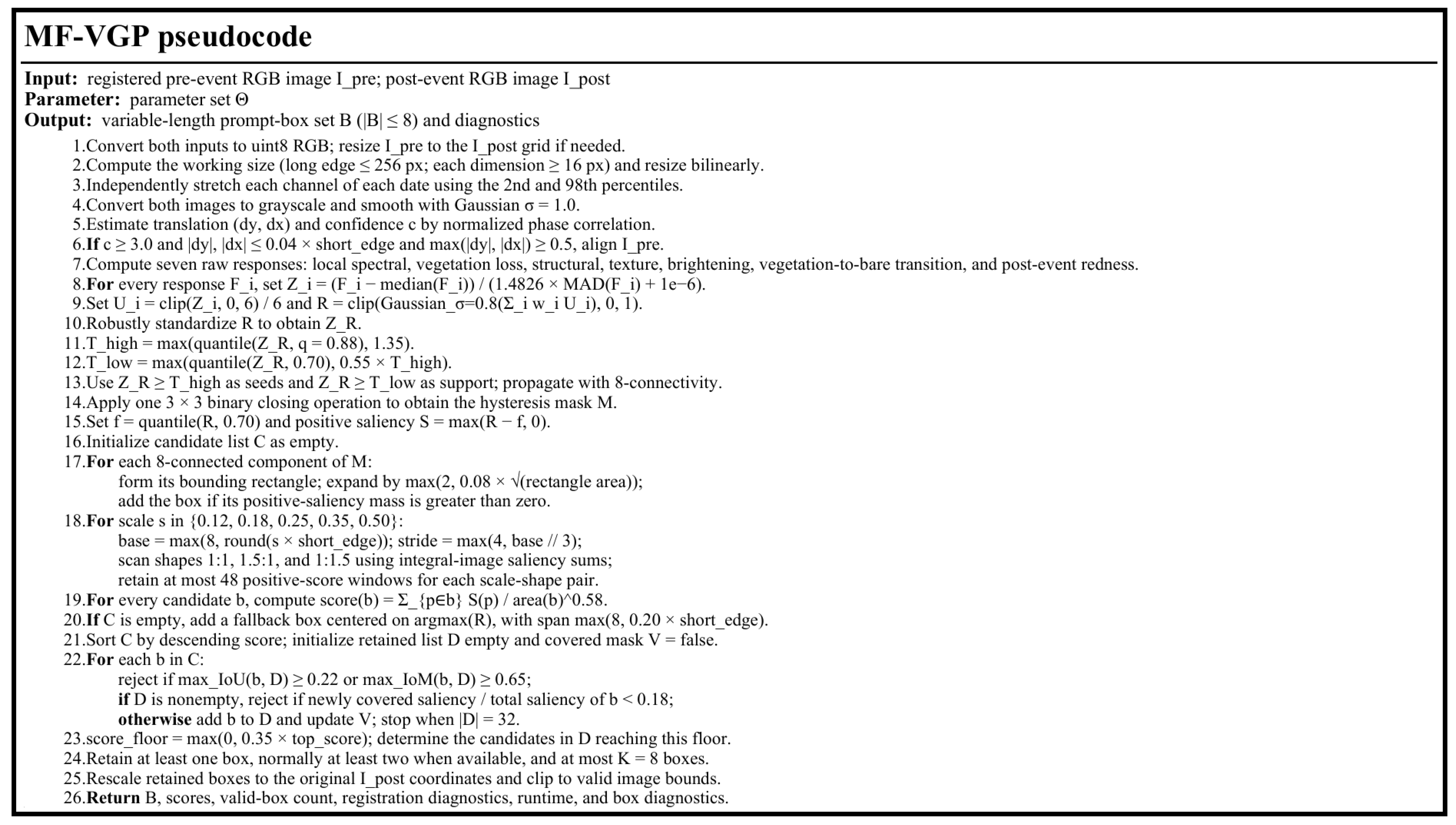
References
- Sun, W.; Bocchini, P.; Davison, B.D. Applications of Artificial Intelligence for Disaster Management. Nat. Hazards 2020, 103, 2631–2689. [Google Scholar] [CrossRef] [Scilit]
- Ghorbanzadeh, O.; Crivellari, A.; Ghamisi, P.; Shahabi, H.; Blaschke, T. A Comprehensive Transferability Evaluation of U-Net and ResU-Net for Landslide Detection from Sentinel-2 Data (Case Study Areas from Taiwan, China, and Japan). Sci. Rep. 2021, 11, 14629. [Google Scholar] [CrossRef] [Scilit] [PubMed]
- He, H.; Zheng, D.; Xu, G.; Dong, X.; Liu, W.; Zou, Y.; Wang, H. Research on the Evolution Mechanisms and Prevention Countermeasures behind a Large-Scale Landslide in Complicated-Geological-Structure Red Beds. Sci. Rep. 2025, 15, 40294. [Google Scholar] [CrossRef] [Scilit] [PubMed]
- Jiang, H.; Ding, M.; Li, L.; Huang, W. Global Dynamic Landslide Susceptibility Modeling Based on ResNet18: Revealing Large-Scale Landslide Hazard Evolution Trends in China. Appl. Sci. 2025, 15, 2038. [Google Scholar] [CrossRef] [Scilit]
- Mohan, A.; Singh, A.K.; Kumar, B.; Dwivedi, R. Review on Remote Sensing Methods for Landslide Detection Using Machine and Deep Learning. Trans. Emerg. Telecommun. Technol. 2021, 32, e3998. [Google Scholar] [CrossRef] [Scilit]
- Geirhos, R.; Jacobsen, J.H.; Michaelis, C.; Zemel, R.; Brendel, W.; Bethge, M.; Wichmann, F.A. Shortcut Learning in Deep Neural Networks. Nat. Mach. Intell. 2020, 2, 665–673. [Google Scholar] [CrossRef] [Scilit]
- Kirillov, A.; Mintun, E.; Ravi, N.; Mao, H.; Rolland, C.; Gustafson, L.; Xiao, T.; Whitehead, S.; Berg, A.C.; Lo, W.-Y.; et al. Segment Anything. In Proceedings of the IEEE/CVF International Conference on Computer Vision, Paris, France, 1–6 October 2023; pp. 4015–4026. [Google Scholar]
- Fiorucci, F.; Ardizzone, F.; Mondini, A.C.; Viero, A.; Guzzetti, F. Visual Interpretation of Stereoscopic NDVI Satellite Images to Map Rainfall-Induced Landslides. Landslides 2019, 16, 165–174. [Google Scholar] [CrossRef] [Scilit]
- Luetzenburg, G.; Svennevig, K.; Bjørk, A.A.; Keiding, M.; Kroon, A. A National Landslide Inventory of Denmark. Earth Syst. Sci. Data 2022, 14, 3157–3165. [Google Scholar] [CrossRef] [Scilit]
- Bai, D.; Tang, J.; Lu, G.; Zhu, Z.; Liu, T.; Fang, J. The Design and Application of Landslide Monitoring and Early Warning System Based on Microservice Architecture. Geomat. Nat. Hazards Risk 2020, 11, 928–948. [Google Scholar] [CrossRef] [Scilit]
- Zhang, L.; Dai, K.; Deng, J.; Ge, D.; Liang, R.; Li, W.; Xu, Q. Identifying Potential Landslides by Stacking-InSAR in Southwestern China and Its Performance Comparison with SBAS-InSAR. Remote Sens. 2021, 13, 3662. [Google Scholar] [CrossRef] [Scilit]
- Liu, H.; Duan, P.; Li, J.; Zhao, K.; Yu, X. Earthquake Landslide Detection Method Combining Post-Earthquake Coherence Increase and Polarized Vegetation Damage. Geomat. Nat. Hazards Risk 2025, 16, 2492329. [Google Scholar] [CrossRef] [Scilit]
- Ageenko, A.; Hansen, L.C.; Lyng, K.L.; Bodum, L.; Arsanjani, J.J. Landslide Susceptibility Mapping Using Machine Learning: A Danish Case Study. ISPRS Int. J. Geo-Inf. 2022, 11, 324. [Google Scholar] [CrossRef] [Scilit]
- Lu, P.; Qin, Y.; Li, Z.; Mondini, A.C.; Casagli, N. Landslide Mapping from Multi-Sensor Data through Improved Change Detection-Based Markov Random Field. Remote Sens. Environ. 2019, 231, 111235. [Google Scholar] [CrossRef] [Scilit]
- Chen, L.; Xiao, J.; Zhang, Y. Improve Unsupervised Learning-Based Landslides Detection by Band Ratio Processing of RGB Optical Images: A Case Study on Rainfall-Induced Landslide Clusters. Geomat. Nat. Hazards Risk 2024, 15, 2363406. [Google Scholar] [CrossRef] [Scilit]
- Cheng, G.; Han, J.; Lu, X. Remote Sensing Image Scene Classification: Benchmark and State of the Art. Proc. IEEE 2017, 105, 1865–1883. [Google Scholar] [CrossRef] [Scilit]
- Xia, G.-S.; Bai, X.; Ding, J.; Zhu, Z.; Belongie, S.; Luo, J.; Datcu, M.; Pelillo, M.; Zhang, L. DOTA: A Large-Scale Dataset for Object Detection in Aerial Images. In Proceedings of the IEEE Conference on Computer Vision and Pattern Recognition (CVPR), Salt Lake City, UT, USA, 18–23 June 2018; pp. 3974–3983. [Google Scholar] [CrossRef] [Scilit]
- Daudt, R.C.; Le Saux, B.; Boulch, A. Fully Convolutional Siamese Networks for Change Detection. In Proceedings of the 2018 25th IEEE International Conference on Image Processing (ICIP), Athens, Greece, 7–10 October 2018; pp. 4063–4067. [Google Scholar] [CrossRef] [Scilit]
- Xiao, Y.; Yuan, Q.; Jiang, K.; He, J.; Lin, C.-W.; Zhang, L. TTST: A Top-k Token Selective Transformer for Remote Sensing Image Super-Resolution. IEEE Trans. Image Process. 2024, 33, 738–752. [Google Scholar] [CrossRef] [Scilit] [PubMed]
- Ji, S.; Yu, D.; Shen, C.; Li, W.; Xu, Q. Landslide Detection from an Open Satellite Imagery and Digital Elevation Model Dataset Using Attention Boosted Convolutional Neural Networks. Landslides 2020, 17, 1337–1352. [Google Scholar] [CrossRef] [Scilit]
- Shi, W.; Zhang, M.; Ke, H.; Fang, X.; Zhan, Z.; Chen, S. Landslide Recognition by Deep Convolutional Neural Network and Change Detection. IEEE Trans. Geosci. Remote Sens. 2021, 59, 4654–4672. [Google Scholar] [CrossRef] [Scilit]
- Ronneberger, O.; Fischer, P.; Brox, T. U-Net: Convolutional Networks for Biomedical Image Segmentation. In Proceedings of the Medical Image Computing and Computer-Assisted Intervention—MICCAI 2015; Springer: Cham, Switzerland, 2015; Volume 9351, pp. 234–241. [Google Scholar]
- Meena, S.R.; Soares, L.P.; Grohmann, C.H.; van Westen, C.; Bhuyan, K.; Singh, R.P.; Floris, M.; Catani, F. Landslide Detection in the Himalayas Using Machine Learning Algorithms and U-Net. Landslides 2022, 19, 1209–1229. [Google Scholar] [CrossRef] [Scilit]
- Diakogiannis, F.I.; Waldner, F.; Caccetta, P.; Wu, C. ResUNet-a: A Deep Learning Framework for Semantic Segmentation of Remotely Sensed Data. ISPRS J. Photogramm. Remote Sens. 2020, 162, 94–114. [Google Scholar] [CrossRef] [Scilit]
- Prakash, N.; Manconi, A.; Loew, S. Mapping Landslides on EO Data: Performance of Deep Learning Models vs. Traditional Machine Learning Models. Remote Sens. 2020, 12, 346. [Google Scholar] [CrossRef] [Scilit]
- Ghorbanzadeh, O.; Shahabi, H.; Crivellari, A.; Homayouni, S.; Blaschke, T.; Ghamisi, P. Landslide Detection Using Deep Learning and Object-Based Image Analysis. Landslides 2022, 19, 929–939. [Google Scholar] [CrossRef] [Scilit]
- Ren, S.; He, K.; Girshick, R.; Sun, J. Faster R-CNN: Towards Real-Time Object Detection with Region Proposal Networks. In Proceedings of the Advances in Neural Information Processing Systems 28; Neural Information Processing Systems Foundation, Inc.: South Lake Tahoe, NV, USA, 2015; pp. 91–99. [Google Scholar]
- Li, H.; He, Y.; Xu, Q.; Deng, J.; Li, W.; Wei, Y. Detection and Segmentation of Loess Landslides via Satellite Images: A Two-Phase Framework. Landslides 2022, 19, 673–686. [Google Scholar] [CrossRef] [Scilit]
- He, K.; Gkioxari, G.; Dollár, P.; Girshick, R. Mask R-CNN. In Proceedings of the IEEE International Conference on Computer Vision, Venice, Italy, 22–29 October 2017; pp. 2961–2969. [Google Scholar]
- Liu, X.; Xu, L.; Zhang, J. Landslide Detection with Mask R-CNN Using Complex Background Enhancement Based on Multi-Scale Samples. Geomat. Nat. Hazards Risk 2024, 15, 2300823. [Google Scholar] [CrossRef] [Scilit]
- Chen, S.; Ge, C.; Tong, Z.; Wang, J.; Song, Y.; Wang, J.; Luo, P. AdaptFormer: Adapting Vision Transformers for Scalable Visual Recognition. In Proceedings of the Advances in Neural Information Processing Systems 35; Neural Information Processing Systems Foundation, Inc.: South Lake Tahoe, NV, USA, 2022; pp. 16664–16678. [Google Scholar]
- Jia, M.; Tang, L.; Chen, B.-C.; Cardie, C.; Belongie, S.; Hariharan, B.; Lim, S.-N. Visual Prompt Tuning. In Proceedings of the European Conference on Computer Vision; Springer: Cham, Switzerland, 2022; Volume 13693, pp. 709–727. [Google Scholar]
- Zhang, J.; Huang, J.; Jin, S.; Lu, S. Vision-Language Models for Vision Tasks: A Survey. IEEE Trans. Pattern Anal. Mach. Intell. 2024, 46, 5625–5644. [Google Scholar] [CrossRef] [Scilit] [PubMed]
- Xi, L.; Yu, J.; Ge, D.; Pang, Y.; Zhou, P.; Hou, C.; Li, Y.; Chen, Y.; Dong, Y. SAM-CFFNet: SAM-Based Cross-Feature Fusion Network for Intelligent Identification of Landslides. Remote Sens. 2024, 16, 2334. [Google Scholar] [CrossRef] [Scilit]
- Yang, B.; Chen, Y.; Ghamisi, P. LVM-StARS: Large Vision Model Soft Adaption for Remote Sensing Scene Classification. IEEE Geosci. Remote Sens. Lett. 2024, 21, 6013905. [Google Scholar] [CrossRef] [Scilit]
- Tang, J.; Guo, S.; Tong, B.; Lei, D.; Gao, W.; Liu, Y.; Zhang, N.; Liu, J. LS-FPSAM: A SAM-Based Frequency-Prompt Model for Coseismic Landslide Detection. Geomat. Nat. Hazards Risk 2026, 17, 2652591. [Google Scholar] [CrossRef] [Scilit]
- Oh, J.; Yun, C. Provable Benefit of Cutout and CutMix for Feature Learning. In Proceedings of the Advances in Neural Information Processing Systems 37; Neural Information Processing Systems Foundation, Inc.: South Lake Tahoe, NV, USA, 2024; pp. 114656–114743. [Google Scholar]
- Tong, L.; Qi, S.; An, G.; Liu, C. Large Scale Geo-Hazards Investigation by Remote Sensing in Himalayan Region; Science Press: Beijing, China, 2013. [Google Scholar]
- Ren, Y.; Huang, J.; Hong, Z.; Lu, W.; Yin, J.; Zou, L.; Shen, X. Image-Based Concrete Crack Detection in Tunnels Using Deep Fully Convolutional Networks. Constr. Build. Mater. 2020, 234, 117367. [Google Scholar] [CrossRef] [Scilit]
- Li, Y. The Research on Landslide Detection in Remote Sensing Images Based on Improved DeepLabv3+ Method. Sci. Rep. 2025, 15, 7957. [Google Scholar] [CrossRef] [Scilit] [PubMed]
- Zhang, R.; Jiang, Z.; Guo, Z.; Yan, S.; Pan, J.; Ma, X.; Dong, H.; Gao, P.; Li, H. Personalize Segment Anything Model with One Shot. In Proceedings of the International Conference on Learning Representations 2024 (ICLR 2024), Vienna, Austria, 7–11 May 2024. [Google Scholar]
- Wang, X.; Zhang, X.; Cao, Y.; Wang, W.; Shen, C.; Huang, T. SegGPT: Segmenting Everything in Context. arXiv 2023, arXiv:2304.03284. [Google Scholar]
- Ke, L.; Ye, M.; Danelljan, M.; Tai, Y.-W.; Tang, C.-K.; Yu, F. Segment Anything in High Quality. In Proceedings of the Advances in Neural Information Processing Systems 36; Neural Information Processing Systems Foundation, Inc.: South Lake Tahoe, NV, USA, 2023; pp. 29914–29934. [Google Scholar]
- Xu, Y.; Ouyang, C.; Xu, Q.; Wang, D.; Zhao, B.; Luo, Y. CAS Landslide Dataset: A Large-Scale and Multisensor Dataset for Deep Learning-Based Landslide Detection. Sci. Data 2024, 11, 12. [Google Scholar] [CrossRef] [Scilit] [PubMed]
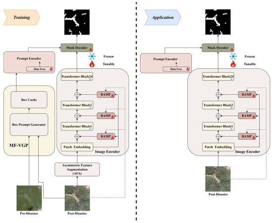
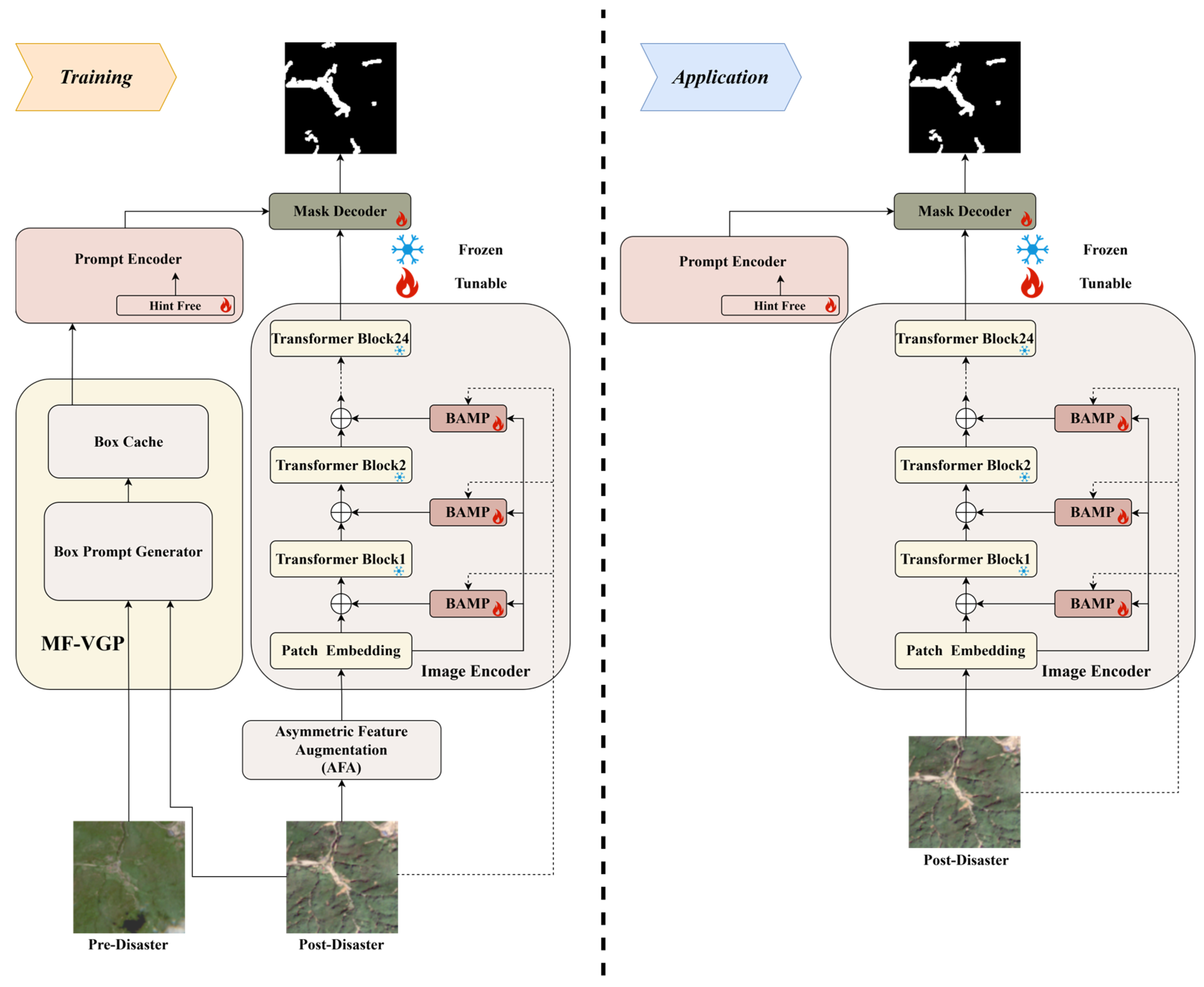
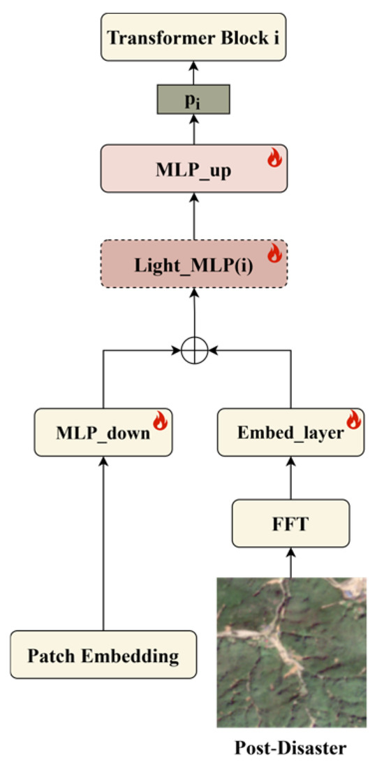
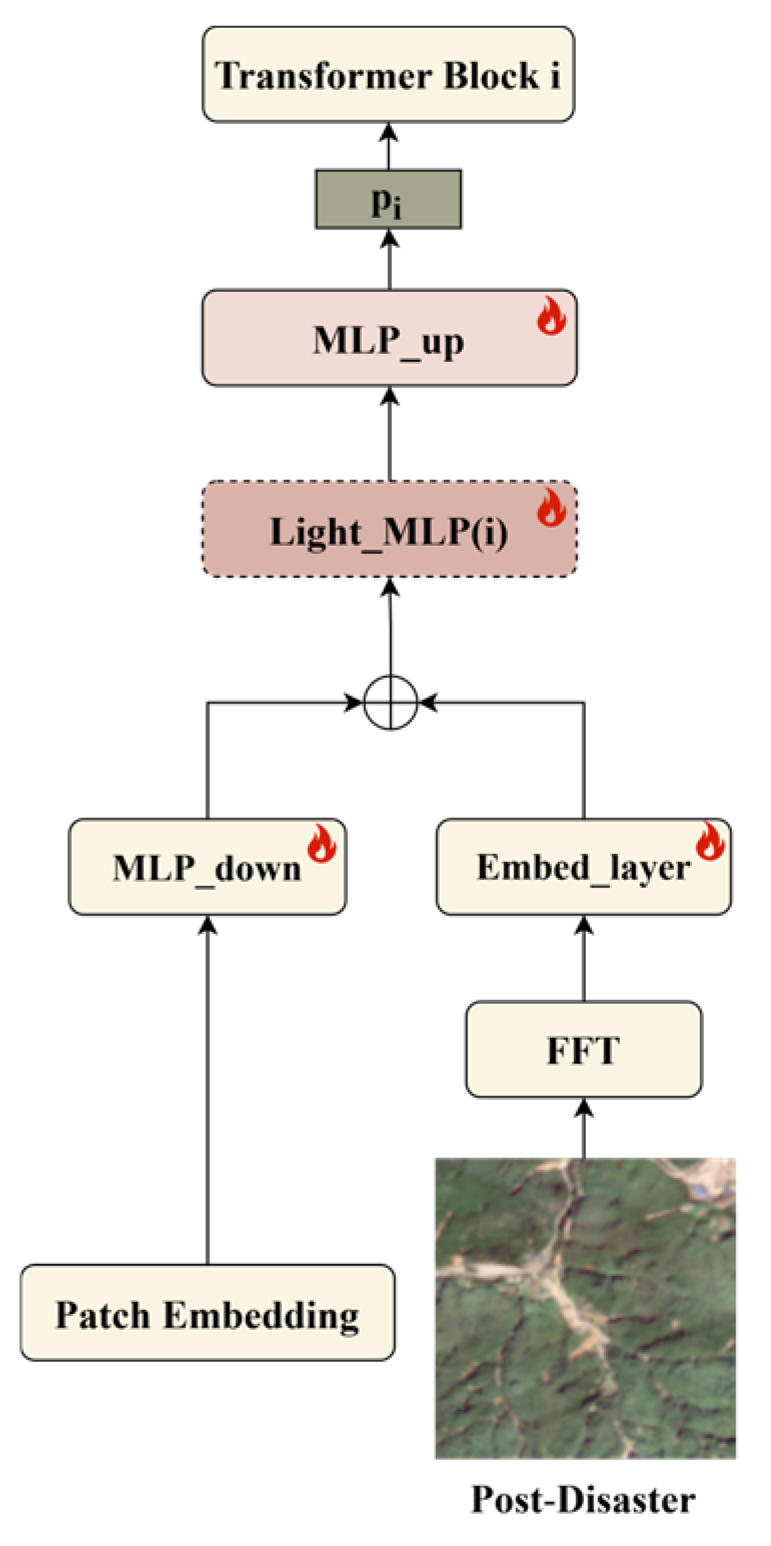
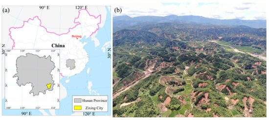
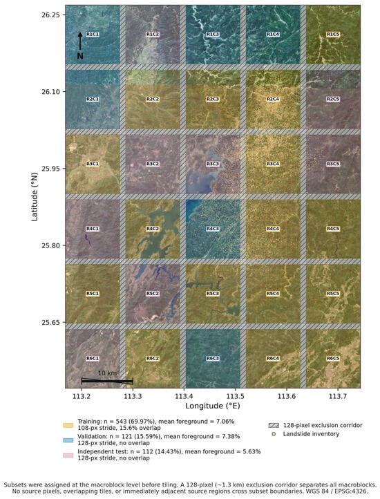
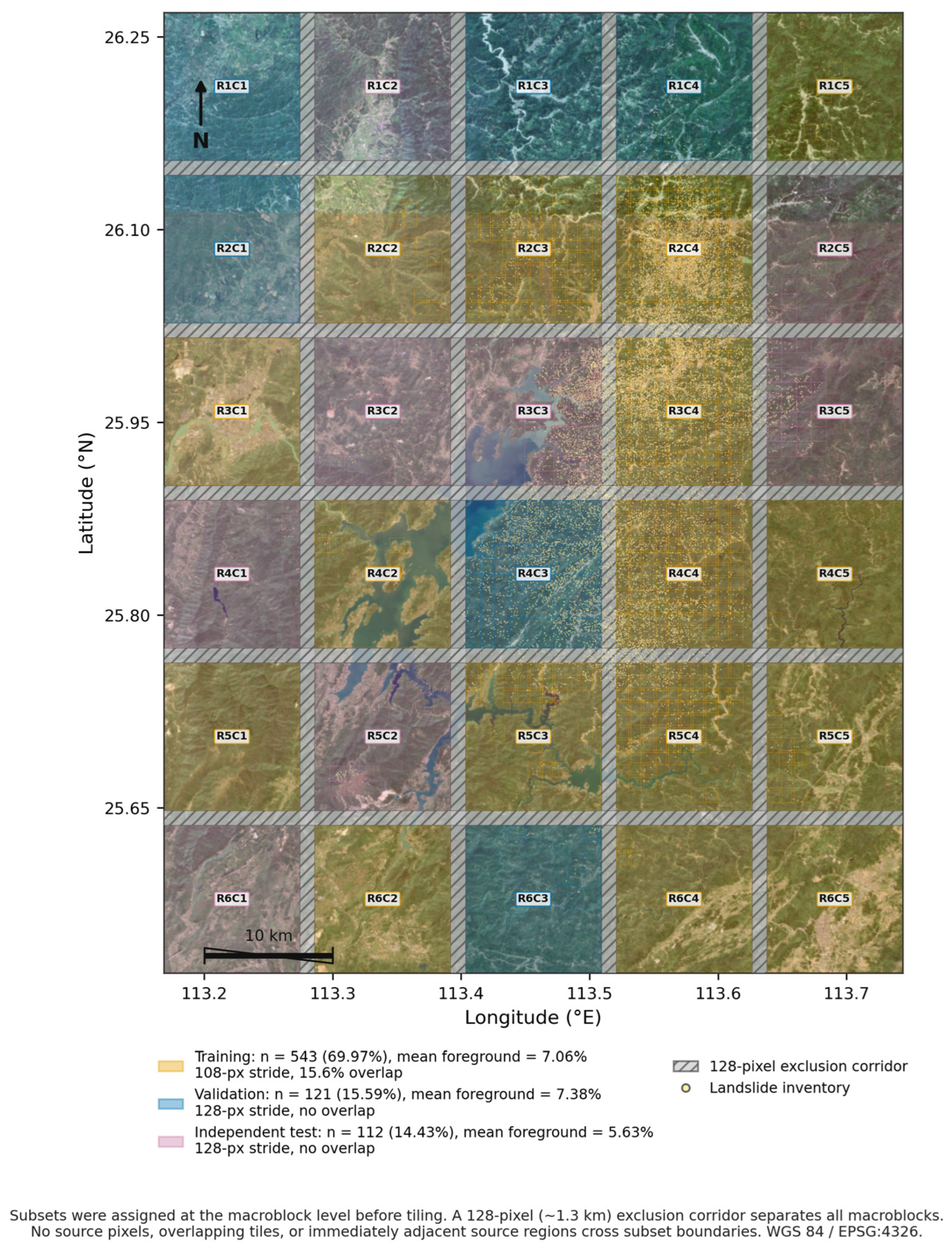
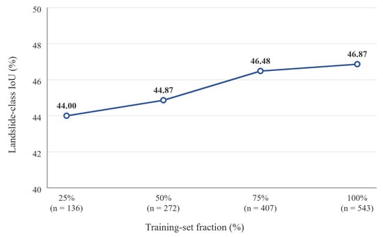
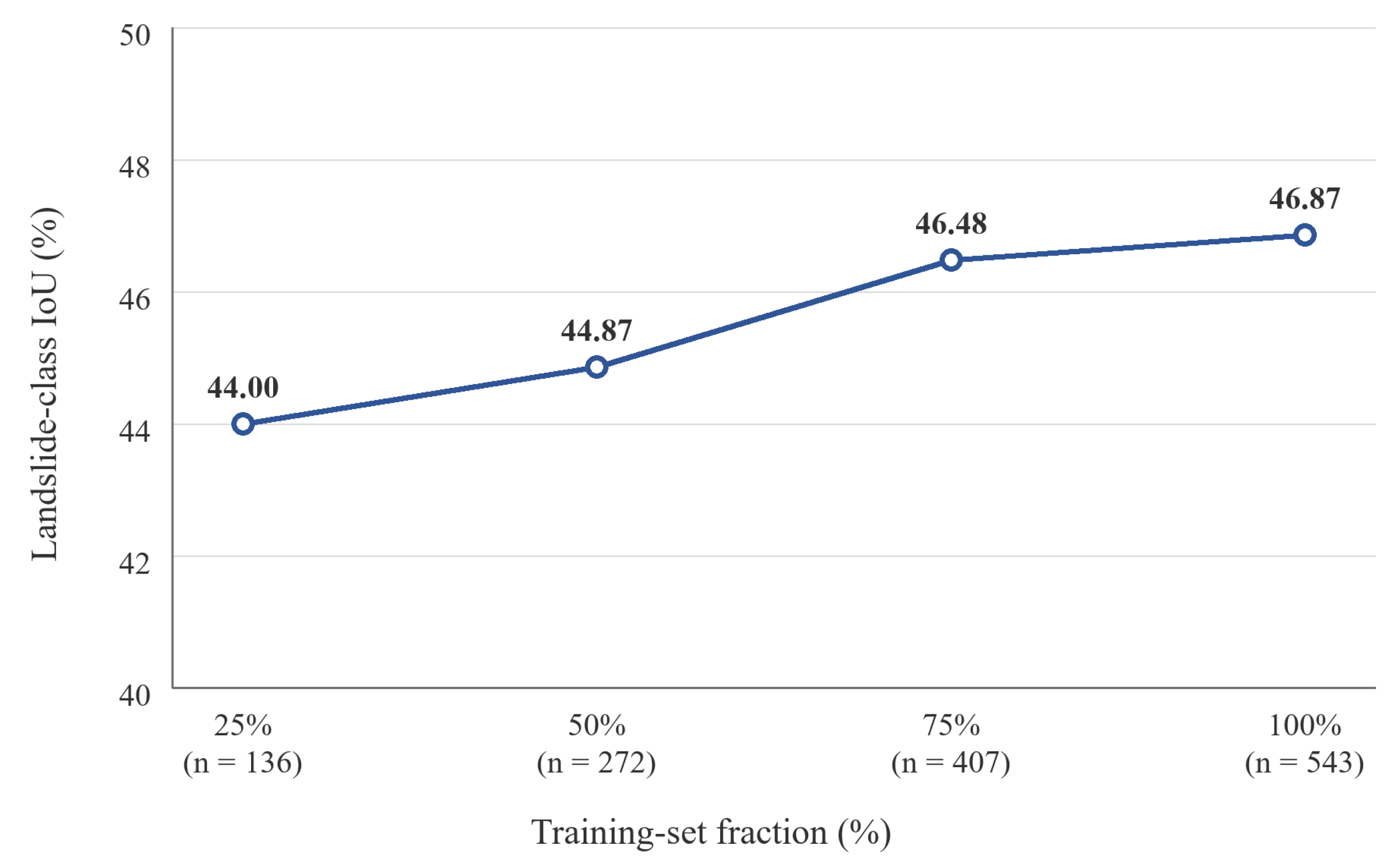
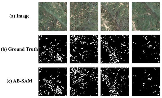
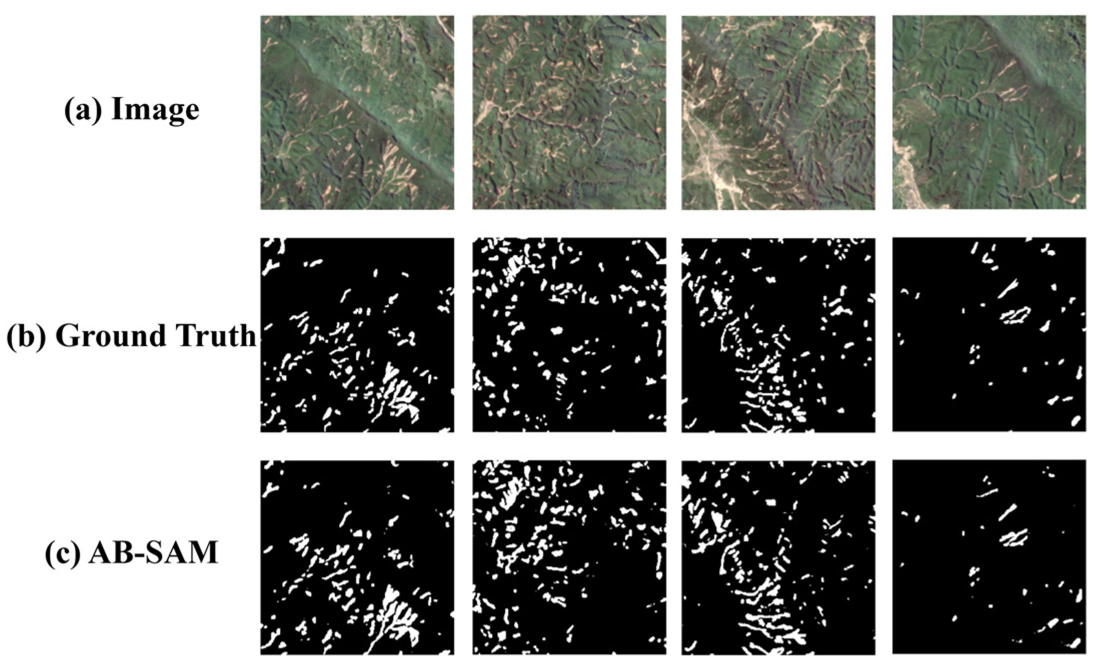
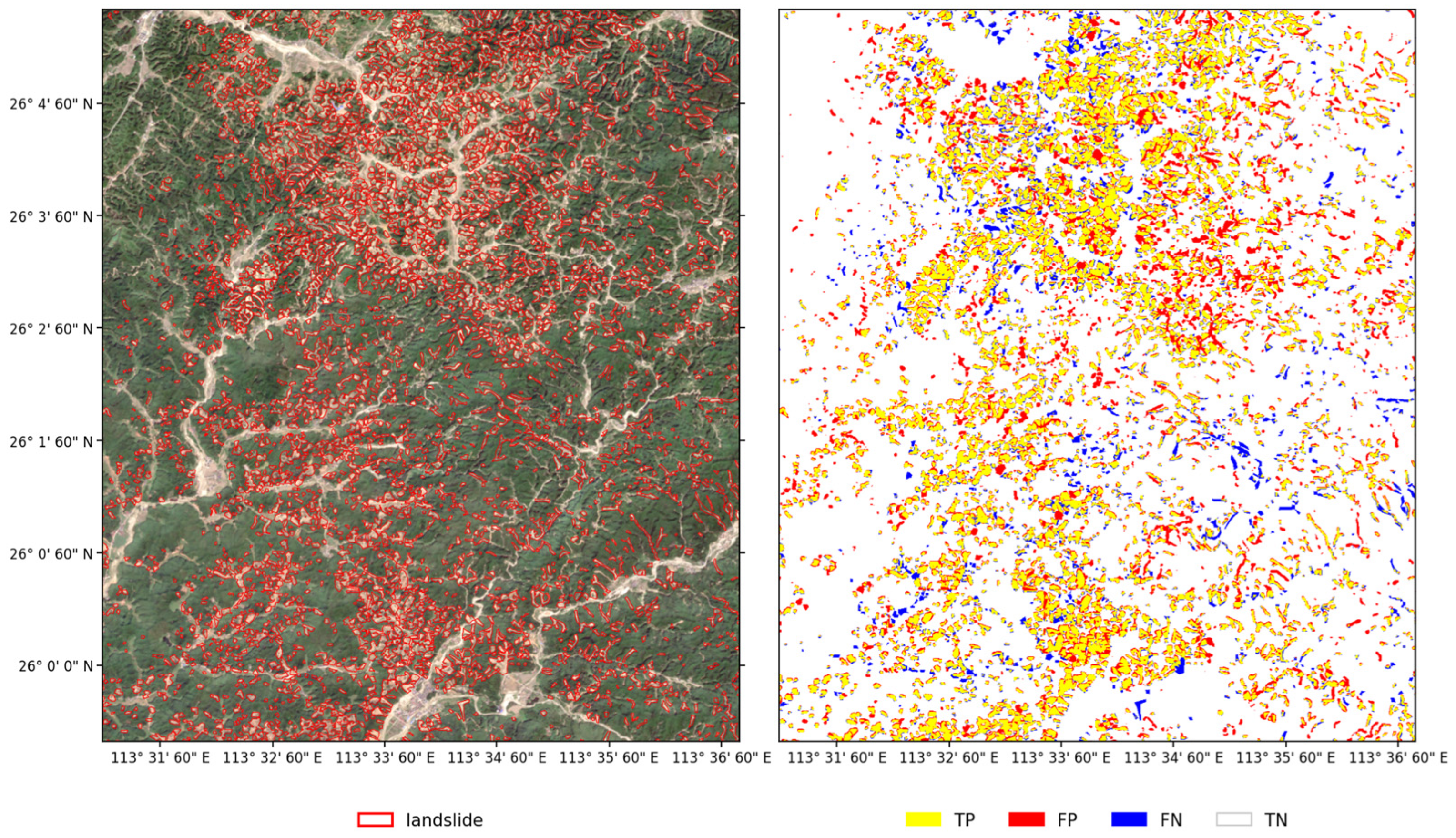
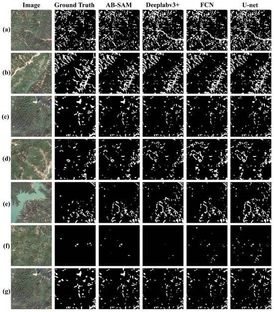
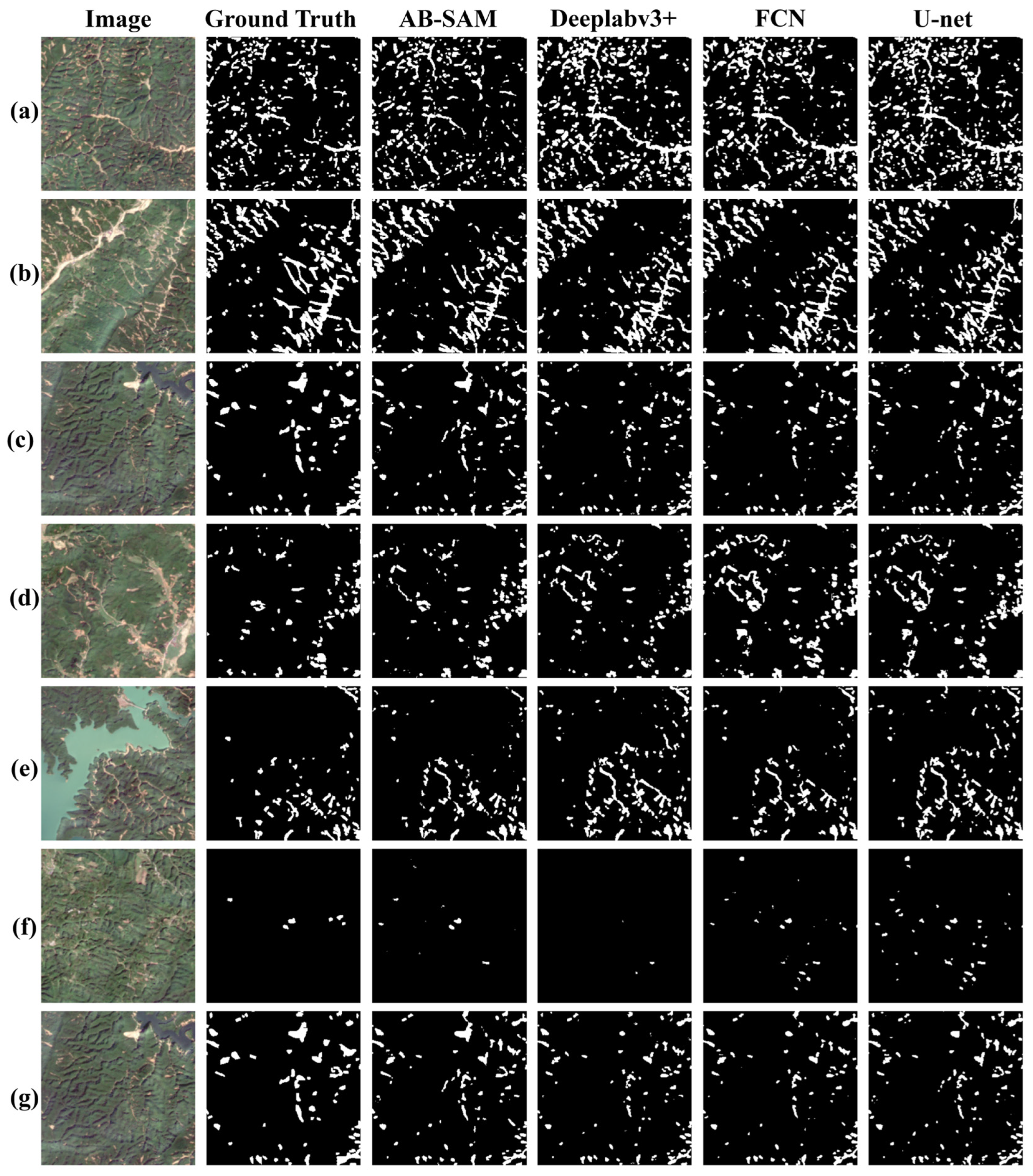


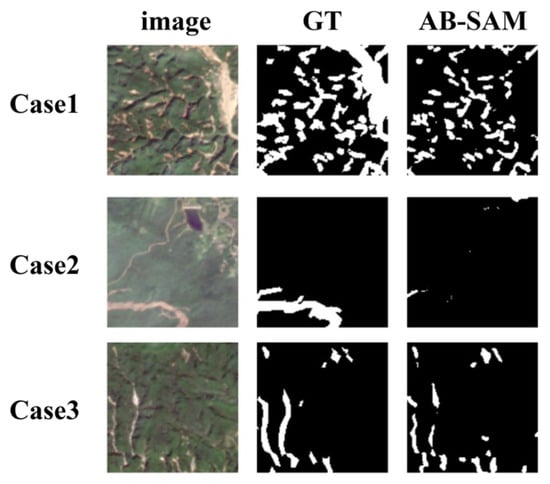
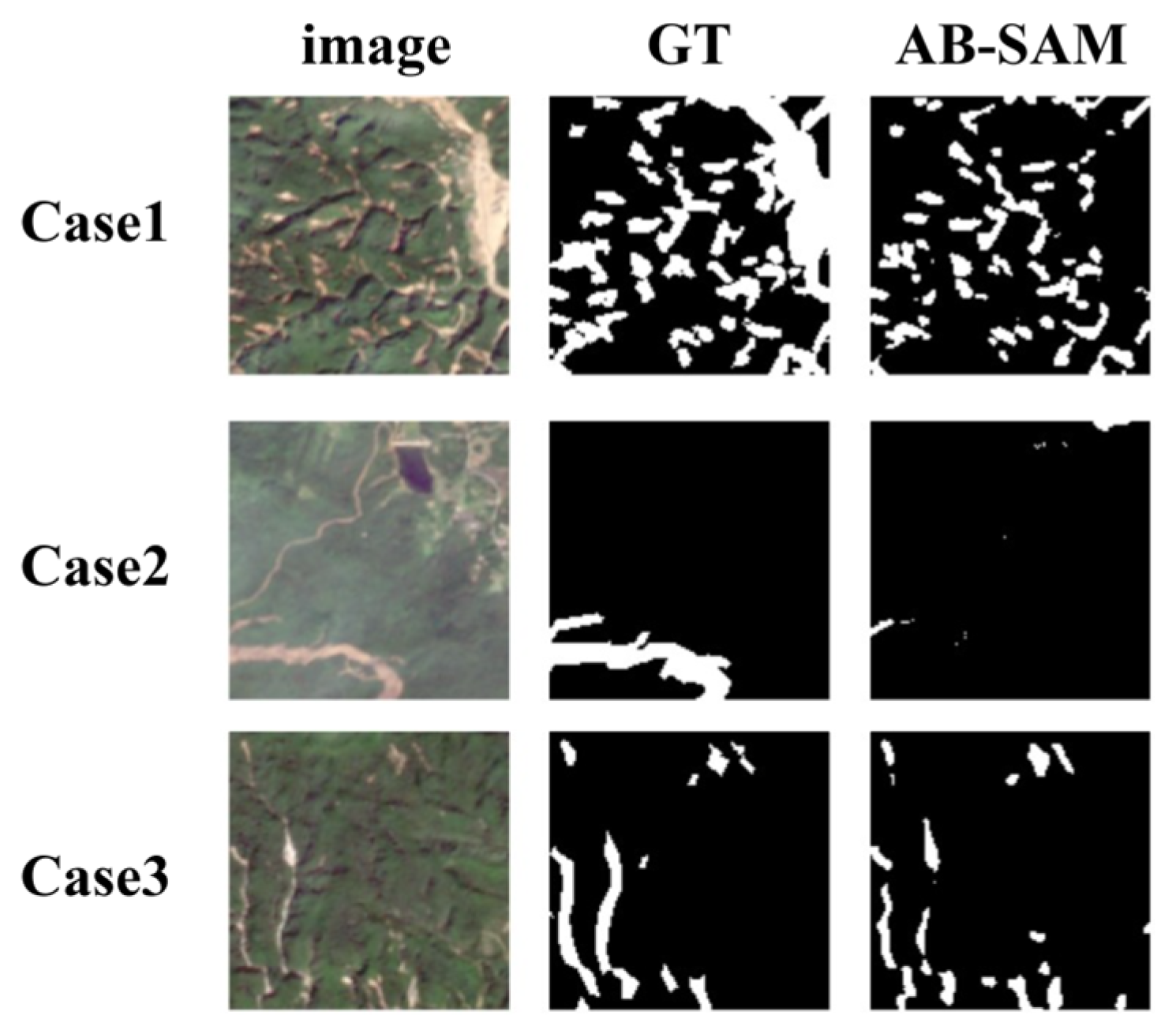

Disclaimer/Publisher’s Note: The statements, opinions and data contained in all publications are solely those of the individual author(s) and contributor(s) and not of MDPI and/or the editor(s). MDPI and/or the editor(s) disclaim responsibility for any injury to people or property resulting from any ideas, methods, instructions or products referred to in the content. |
© 2026 by the authors. Licensee MDPI, Basel, Switzerland. This article is an open access article distributed under the terms and conditions of the Creative Commons Attribution (CC BY) license.