Efficient Mapping of Agricultural Greenhouses in Japan Through Integration of PlanetScope Imagery and Farmland Polygon Data

Abstract

Accurate identification of the spatial distribution of agricultural greenhouses is essential for regional agricultural management in Japan. However, an efficient method for systematically mapping greenhouse locations onto existing farmland maps has not yet been established, and field surveys over large areas require substantial time and labor. This study aims to develop an automated approach for detecting agricultural greenhouses and integrating their locations into farmland maps by combining PlanetScope satellite imagery with farmland polygon data developed by the Japanese government. To improve the efficiency of the extraction process, farmland polygons were used to restrict the analysis to known agricultural areas, thereby reducing false detections originating from non-agricultural land. Within these predefined regions, three machine learning algorithms—Random Forest (RF), Support Vector Machine (SVM), and Isolation Forest (ISF)—were applied to classify and extract greenhouse features from satellite imagery. After optimizing the hyperparameters of all models, RF and SVM achieved an equivalent peak performance, with an F1-score of 0.86, while ISF reached 0.72. RF was, however, markedly more robust to the polygon-level decision threshold, demonstrating a practical advantage in situations where the threshold cannot be optimized in advance. In addition, an ablation experiment confirmed that without pre-masking with farmland polygons, 81.9% of the pixels predicted as greenhouse were distributed outside the agricultural parcels. The proposed method is expected to serve as an effective approach for efficiently identifying the distribution of agricultural facilities and integrating them with existing farmland information in regions characterized by small and fragmented agricultural fields, such as Japan.

1. Introduction

The use of plastic-covered greenhouses (PCGs) in protected agriculture is widely adopted globally as an important technology for precisely controlling the crop growth environment and improving productivity [1]. In regional agricultural management in Japan, understanding the accurate spatial distribution and area of agricultural greenhouses provides essential information for compiling agricultural statistics and infrastructure planning. However, an efficient method for systematically and automatically locating these structures on existing Japanese agricultural maps has not yet been established, and conducting manual field surveys over vast areas presents the challenge of requiring significant time and effort. While plastic covering materials underpin the productivity of protected horticulture, their sustainable use requires improvements in material design and waste management [2]. In addition, greenhouse-led cultivated land has been reported to be increasing continuously in regions such as Shandong Province, China, and understanding its spatial distribution is becoming increasingly important from the perspectives of sustainable agriculture and the ecological environment [3]. Indeed, Global-PCG-10, a 10 m global map of greenhouses derived from Sentinel-2, quantitatively demonstrates that greenhouses are widely distributed throughout the world [4].

Therefore, the development of automated greenhouse extraction methods using satellite remote sensing data, which can observe wide areas simultaneously, has been pursued [1,5]. Although the plastic covering materials used in PCGs have unique optical properties (such as high spectral reflectance), their wavelength characteristics are often similar to those of non-agricultural artifacts and surface features, such as urban buildings (e.g., metal or white roofs) and post-harvest bare land [5]. In particular, agricultural land in Japan is characterized by small, fragmented parcels, and in peri-urban agriculture, these parcels are frequently and complexly mixed with artificial structures such as residential houses and factories. Consequently, traditional pixel-based classification methods that rely solely on the reflectance characteristics of satellite image pixels, without considering the spatial framework of agricultural parcels, carry a high risk of misclassifying surrounding bright artificial structures as greenhouses.

To date, extraction methods using medium-resolution satellite imagery (e.g., Landsat) combined with machine learning [6], as well as object-based methods using high-resolution imagery, have been proposed [7]. However, previous studies have pointed out that medium-resolution imagery with a spatial resolution of 10 to 30 m tends to produce mixed pixels (mixels), where the target feature and surrounding soil or vegetation co-exist within a single pixel, leading to a decrease in extraction accuracy [5,8]. This mixel effect becomes particularly pronounced for the small-scale greenhouses typical of Japanese agricultural lands. Furthermore, even when high-resolution imagery is used in complex environments where diverse land uses are mixed within small areas and spectral characteristics are similar to adjacent non-agricultural artifacts (such as houses and factories), approaches relying solely on spectral and spatial features derived from images struggle to sufficiently eliminate false detections caused by such confusion. Additionally, it has been noted that the utilization of high-frequency, high-spatial-resolution time-series data is effective for capturing crop growth and seasonal land cover changes (phenology) to improve classification accuracy [9]. Greenhouse extraction methods have diversified rapidly in recent years. In addition to object-based classification using Sentinel-2 and SPOT-7 [10] and object-based crop classification by machine learning [11], reported approaches include greenhouse extraction by deep learning from Google Earth and other high-resolution imagery [12,13], large-scale extraction from Sentinel-1/2 that couples prior knowledge with deep learning [14], multitemporal object detection with an improved YOLOX [15], and the combination of two-temporal Sentinel-2 imagery with a one-dimensional convolutional neural network (1D-CNN) [16]. Methods based on spectral indices are also widely used, and a comprehensive benchmarking of the available Sentinel-2 indices [17] and a modified index suited to fragmented terrains [18] have been proposed. Studies exploiting time series and cloud geoprocessing are likewise advancing, including large-scale mapping by ensemble learning on Google Earth Engine [19], annual greenhouse maps derived from long-term Landsat time series [20], discrimination of covered and uncovered agricultural soil [21], and detection of plastic-mulched farmland by time-series machine learning [22]. As [18] points out in particular, mixed pixels exert a strong influence in terrains with subdivided parcels, which suggests that spatially constraining the target area is especially effective for the fragmented agricultural land of Japan.

Therefore, the objective of this study is to develop an automated and efficient greenhouse detection method by combining PlanetScope satellite imagery, which offers a 3 m spatial resolution and high-frequency observation capabilities, with existing agricultural parcel polygon data provided by the Japanese government. The novelty of this study lies in structurally suppressing false detections originating from non-agricultural areas (e.g., buildings) by pre-masking the target area with agricultural polygons in complex peri-urban agricultural landscapes and subsequently applying high-frequency time-series statistics to machine learning algorithms. By constructing time-series statistics that reflect seasonal changes within these designated areas and applying three machine learning algorithms—Random Forest (RF), Support Vector Machine (SVM), and Isolation Forest (ISF)—this study evaluates an approach for efficiently grasping the distribution of agricultural facilities and integrating them with existing agricultural information in the small-scale, fragmented agricultural lands of Japan.

2. Materials and Methods

2.1. Study Area

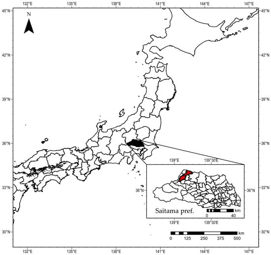
The study area of this research was Honjo City, Japan, which is located at the northwestern edge of Saitama Prefecture and borders Gunma Prefecture, as shown in Figure 1.

Figure 1. Study area. Location of Honjo City, Saitama Prefecture, Japan (red); the inset shows Saitama Prefecture. Coordinates are geographic latitude/longitude (WGS 84); a north arrow and scale bars are provided.

The city features a varied topography, ranging from flat terrain along the Tone River to mountainous areas extending to the outer edges of the Chichibu mountain range, encompassing diverse agricultural fields such as vegetable farms, orchards, and paddy fields. Protected horticulture is also actively practiced, with the production of crops such as cucumbers, strawberries, and flowers. In this study, the agricultural lands in the northern region of the city, where plastic greenhouses for protected horticulture and fields of various crops are concentrated, were selected as the target area for analysis. As this region is adjacent to urbanized areas and diverse land uses are mixed within a small area, it is suitable as a test site for verifying the classification performance and generalizability of agricultural land cover classification models using satellite imagery.

2.2. Satellite Imagery

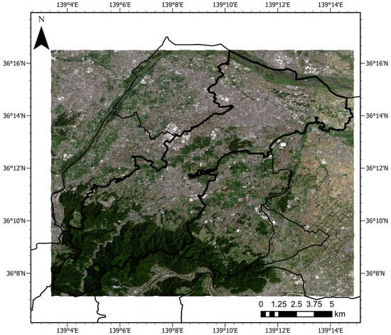
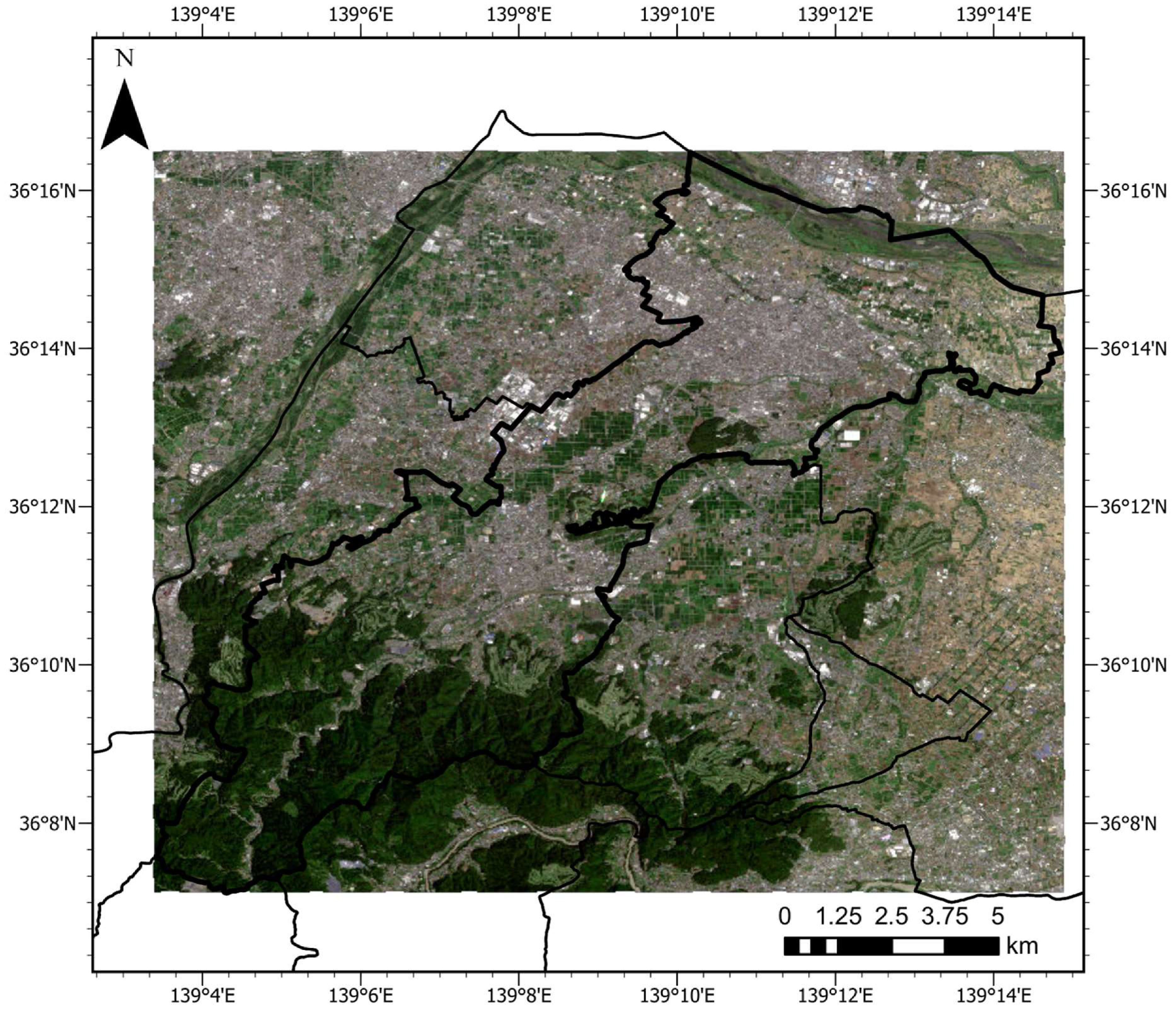
As the observation data for the study area, satellite imagery from the small satellite constellation “PlanetScope (Dove)” operated and provided by Planet Labs (San Francisco, CA, USA), as shown in Figure 2, was adopted.

Figure 2. PlanetScope (Dove) imagery of the study area (Level-3B surface reflectance, 3 m spatial resolution, true color) acquired on 17 August 2024. The bold black line denotes the boundary of Honjo City. Coordinates are geographic latitude/longitude (WGS 84).

The main reason for selecting this image data lies in its combination of “high spatial resolution” and “high-frequency observation” [23]. Although the spatial resolution of imagery is a significant factor in the automated detection of agricultural greenhouses [24], this data, with a spatial resolution of 3 m, enables detailed observation at the level of small agricultural parcels in Japan. Therefore, it is considered suitable for extracting facilities with clear boundaries. Furthermore, high-frequency observation enables the consistent acquisition of year-round time-series data by mitigating the effects of clouds, and it is also suitable for capturing seasonal land cover changes (phenology) in agricultural lands associated with crop planting and harvesting. CubeSat constellations, including PlanetScope, have been shown to capture crop phenology with high accuracy through near-daily observations, for example, in the daily retrieval of leaf area index [25], and are therefore well suited to the extraction of features throughout the year.

Data Specifications: The observation period covered a full year from 5 January to 24 December 2024. The product used was “Level-3B,” which employs data that has been geometrically (ortho-rectified) and radiometrically corrected, and converted to Surface Reflectance. Band Configuration: Data from four wavelength bands—Blue, Green, Red, and Near-Infrared (NIR)—were used. The specifications of the satellite imagery are shown in Table 1, below.

Table 1. Specifications of the satellite imagery used in this study.

Item	Specification
Satellite/Sensor	PlanetScope/Dove
Spatial Resolution	3 m
Band Configuration	4 bands (RGB, NIR)
Observation Period	5 January 2024 to 24 December 2024
Processing Level	Level-3B (Orthorectified), Surface Reflectance (SR)
Data Provider	Planet Labs

2.3. Ground Truth and Reference Data

As the data defining the shapes of agricultural parcels, the agricultural parcel polygon data published by the Ministry of Agriculture, Forestry and Fisheries (MAFF) was used. This is administrative data in which the boundaries of individual agricultural parcels are polygonized based on aerial photographs and other sources. The data contains classifications of agricultural land types, such as upland fields or paddy fields, stored as attribute information.

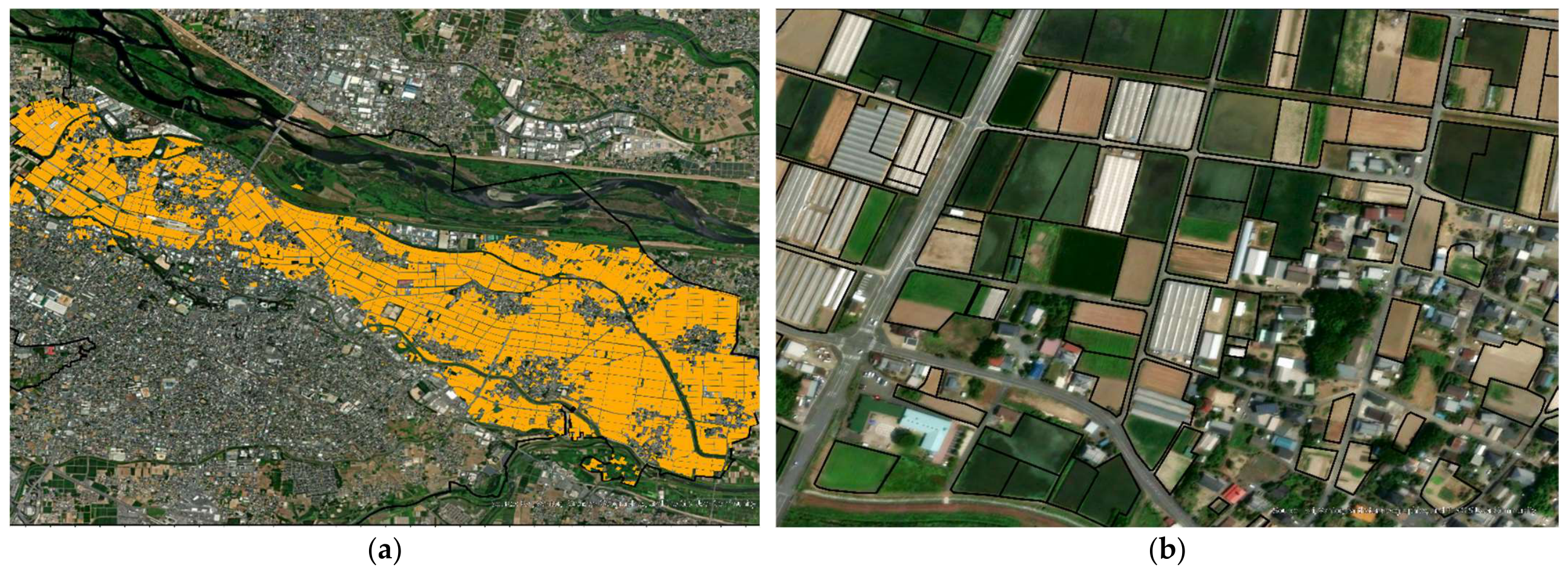
A total of 5025 polygons were extracted from the agricultural polygons within the study area shown in Figure 3. Visual interpretation (annotation) was conducted on the PlanetScope imagery while comparing it with high-resolution satellite imagery (WorldView-3, captured on 22 November 2024) used as ground truth. Furthermore, for parcels where it was difficult to distinguish the presence or type of facilities (e.g., plastic greenhouses versus other artificial structures) using only overhead satellite imagery, Google Earth and Google Street View were used to supplementarily check the on-site conditions, thereby ensuring the reliability of the annotations.

Figure 3. Farmland polygon data: (a) polygons of the entire target region; (b) an enlarged view.

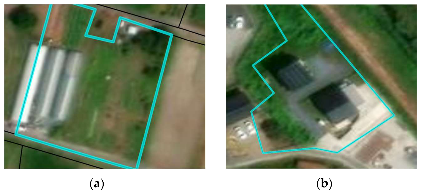
If a facility considered to be a greenhouse occupied 50% or more of the area within a polygon, it was labeled as a “greenhouse” polygon. Cases where a greenhouse was present within a polygon but occupied less than 50% of the area, as shown in Figure 4a, were labeled as “partial greenhouse.” Polygons that are not currently used as agricultural land, as shown in Figure 4b, were labeled as “non-agricultural land”.

Figure 4. Examples of annotated polygons overlaid on satellite imagery. In each panel, the area enclosed by the cyan outline is the agricultural parcel polygon concerned: (a) a polygon labeled as “partial greenhouse”, in which a greenhouse occupies less than 50% of the polygon area; (b) a polygon labeled as “non-agricultural land”.

For polygons where no greenhouses were present, labeling was performed based on the upland field and paddy field classifications stored in the attribute table of the original agricultural polygon data.

As shown in Table 2, the composition of land use types assigned to each polygon was 70.15% (3525 polygons) for upland fields, 16.98% (853 polygons) for paddy fields, 10.67% (536 polygons) for greenhouses, 1.99% (100 polygons) for partial greenhouses, and 0.21% (11 polygons) for non-agricultural land. This labeled data was used as the dataset for training and validation.

Table 2. Annotation results of reference polygons.

Land Use Type	Number of Polygons	Proportion (%)
Upland field	3525	70.15
Paddy field	853	16.98
Greenhouse	536	10.67
Partial greenhouse	100	1.99
Non-agricultural land	11	0.21
Total	5025	100

2.4. Data Preprocessing and Feature Extraction

To accurately classify target objects from the imagery, in addition to the spectral reflectance of each pixel (Blue, Green, Red, NIR), the following two indices were calculated and added as features. Here, ${\rho }_{\mathrm{B}\mathrm{l}\mathrm{u}\mathrm{e}},{\rho }_{\mathrm{G}\mathrm{r}\mathrm{e}\mathrm{e}\mathrm{n}},{\rho }_{\mathrm{R}\mathrm{e}\mathrm{d}} \mathrm{a}\mathrm{n}\mathrm{d} {\rho }_{\mathrm{N}\mathrm{I}\mathrm{R}}$ represent the surface reflectance of the Blue, Green, Red, and Near-Infrared bands, respectively.

NDVI (Normalized Difference Vegetation Index): Adopted as an indicator to detect and identify the growth status of open-field crops and surrounding vegetation [26].

$$\mathrm{N}\mathrm{D}\mathrm{V}\mathrm{I}={\displaystyle \frac{{\rho }_{\mathrm{N}\mathrm{I}\mathrm{R}}-{\rho }_{\mathrm{R}\mathrm{e}\mathrm{d}}}{{\rho }_{\mathrm{N}\mathrm{I}\mathrm{R}}+{\rho }_{\mathrm{R}\mathrm{e}\mathrm{d}}}}$$

(1)

• RPGI (Retrogressive Plastic Greenhouse Index): An index for detecting the optical characteristics of covering materials such as plastic. It was adopted as an important feature directly contributing to the detection of plastic greenhouses, which is the main objective of this study. While the original index proposed by Yang et al. [27] includes the Blue, Green, and NIR bands in the average reflectance of the denominator, the RPGI in this study was calculated using the following formula, in accordance with the definition of a subsequent previous study [28], considering the spectral characteristics of PlanetScope imagery. This formula places the reflectance of the Blue band in the numerator and, in the denominator, the value obtained by subtracting the average reflectance of the Red, Green, and NIR bands from 1:

$$\mathrm{R}\mathrm{P}\mathrm{G}\mathrm{I}={\displaystyle \frac{{\rho }_{\mathrm{B}\mathrm{l}\mathrm{u}\mathrm{e}}}{1-\mathrm{M}\mathrm{e}\mathrm{a}\mathrm{n}\left({\rho }_{\mathrm{R}\mathrm{e}\mathrm{d}}+{\rho }_{\mathrm{G}\mathrm{r}\mathrm{e}\mathrm{e}\mathrm{n}}+{\rho }_{\mathrm{N}\mathrm{I}\mathrm{R}}\right)}}$$

(2)

In this analysis, to evaluate the impact of capturing seasonal variations (phenology) on greenhouse extraction accuracy, two datasets were compared: a “Single-Image Dataset” and a “Time-Series Dataset.” For the Single-Image Dataset, a clear day with no cloud cover in the study area, 17 August 2024, was selected. It was considered that an image from this period would be effective for classification because the strong solar radiation (light intensity) typical of summer makes the optical contrast between actively growing surrounding vegetation (open-field crops) and plastic greenhouses most distinct. A total of six dimensions, consisting of the four-band reflectances and the two indices from this single image, were directly input as features. On the other hand, for the dataset handling year-round time-series data (January to December 2024), imagery from a total of 24 dates with low cloud cover was used. The screening criterion was that cloud cover over the study area be 10% or less. The 24 selected dates span January to December 2024 and are distributed almost evenly, with approximately two dates per month (one in February and three in March), so that seasonal variation (phenology) is captured without bias throughout the year. For the reflectance of each pixel and each index, statistics including the maximum (Max), minimum (Min), standard deviation (Std), and mean (Mean) over the period were calculated, resulting in a total of 24 dimensions. Using only a single-date image tends to cause misclassifications with features that exhibit reflection characteristics similar to greenhouses at specific times (e.g., bare land immediately after harvest or white buildings) [5]. Therefore, the intention was to have the model learn seasonal land cover changes due to planting and harvesting as year-round statistics, thereby improving the accuracy of discrimination from static artificial structures and open-field crops based on temporal variation patterns (phenology) [9].

2.5. Classification Algorithms and Polygon-Level Decision

To perform classification using the calculated features, three types of machine learning algorithms were adopted to compare their classification performance: RF, SVM, and ISF, which is an anomaly detection method. The reasons for selecting each method are as follows. RF is an ensemble learning algorithm combining decision trees [29] and is less prone to overfitting even for multidimensional data with non-linear relationships. Additionally, it has the characteristic of showing stable performance with relatively little parameter tuning in the classification of remote sensing data [30] and has been shown to be effective in agricultural infrastructure and land surface classification [7]. SVM is excellent at determining complex boundaries in high-dimensional spaces and is widely utilized in the remote sensing field [31]; therefore, it was selected as a comparative method for supervised learning. Furthermore, because the dataset in this study is imbalanced, with greenhouse polygons accounting for approximately 11% of all 5014 polygons, the application of ISF [32] was attempted as an approach to separate and detect the minority greenhouse pixels as anomalies in the data space from the majority surrounding agricultural land (normal values).

The dataset was divided using a stratified split at the polygon level, with 60% of the total polygons used as training data, 20% as validation data, and the remaining 20% as test data. To prevent data leakage, the polygon-level split ensured that pixels from the same agricultural polygon were not distributed across more than one of these sets. Upon training the models, the composition of the training data was modified according to the characteristics of each algorithm. In the supervised learning methods, RF and SVM, pixels of pure classes—“upland fields,” “paddy fields,” and “greenhouses”—were used for training, excluding the “partial greenhouse” class. This is because the polygons of “partial greenhouses” contain many pixels consisting of elements other than greenhouses, which obscures the boundaries of features during model training and causes a decrease in classification accuracy. At the evaluation stage, however, in line with the practical objective of compiling a parcel-level greenhouse inventory, “partial greenhouse” was merged into the “with greenhouse” class in the polygon-level ground truth; that is, the class was excluded from training in order to obtain pure pixel features, whereas the evaluation was based on whether or not a parcel contains a greenhouse. In addition, “non-agricultural land” polygons accounted for only 0.21% of the total (11 parcels) and, because the proposed method by its nature targets agricultural parcels, they were excluded from both training and evaluation.

The hyperparameters of the supervised learning methods (RF and SVM) were both optimized by grid search (GridSearchCV) in order to ensure fairness of comparison. Polygon-level cross-validation (GroupKFold with three folds) was used so that pixels of the same polygon were not distributed across the training and validation folds. For RF, the number of decision trees (n_estimators) and the maximum tree depth (max_depth) were searched; for SVM with a radial basis function (RBF) kernel, the regularization parameter C and the kernel coefficient gamma were searched. Because SVM is distance-based, all features were standardized, and the training pixels were subsampled for computational reasons. Weighting for class imbalance (class_weight = ‘balanced’) was applied to both models. As a result of the search, the optimal parameters were max_depth = 20 and n_estimators = 200 for RF with the single-image dataset, max_depth = 20 and n_estimators = 100 for RF with the time-series dataset, C = 1 and gamma = 0.1 for SVM with the single-image dataset, and C = 1 and gamma = scale for SVM with the time-series dataset.

In addition, an ablation experiment comparing the presence and absence of masking was conducted in order to verify the contribution of the pre-masking step based on the agricultural polygons. The best model (RF with time-series features) was applied pixel-wise to all pixels within the bounding box of the polygon set, without constraining it to the agricultural polygons, and the pixels predicted as greenhouse were tabulated according to whether they fell inside or outside the agricultural polygons.

On the other hand, for ISF, a semi-supervised anomaly detection approach was adopted in which the “greenhouse” class was also excluded from the training data, and only the distribution of normal pixels of “upland fields” and “paddy fields” was learned. The parameters of the ISF were likewise searched exhaustively over the contamination rate (0.001, 0.005, 0.01, 0.05, 0.1), max_samples (auto, 256, 512), and the number of decision trees, n_estimators (100, 200, 300), and the combination that maximized the greenhouse-extraction F1-score on the validation data was selected. As a result of the search, contamination = 0.01, max_samples = auto, and n_estimators = 300 were adopted (validation F1 = 0.835). It should be noted that the contamination parameter of the ISF is not an estimate of the proportion of greenhouses in the dataset. Because, in this study, the ISF is trained only on the normal pixels of “upland fields” and “paddy fields,” the outlier rate of the training set is by construction close to zero, and contamination acts as an offset of the decision boundary on the anomaly score. The actual class imbalance is absorbed by the subsequent polygon-level decision threshold (14% for this model; see Section 3.3) in this two-stage design. Indeed, increasing contamination to 0.05 and 0.1 causes normal pixels to be over-flagged as outliers, and the validation F1-score falls to 0.816 and 0.769, respectively, so that 0.01 was the best value. Pixels determined to be outliers in the prediction were treated as “greenhouses.” The ISF was evaluated using the same 24 acquisition dates, the same stratified three-way split, and the same test polygons as RF and SVM (1003 parcels, of which 127 are positive after merging “greenhouse” and “partial greenhouse”), so that the three methods could be compared under identical conditions.

As a feature of the classification process, prediction was first executed on a pixel-by-pixel basis, discriminating whether each pixel was a “greenhouse” or “non-greenhouse.” Subsequently, considering practicality in agricultural fields, the results were aggregated into the agricultural polygon units defined in Section 2.3. The final decision for each polygon is made using a threshold on the proportion of pixels within the polygon that are predicted as greenhouse. In this study, this threshold was not fixed at an empirical value; instead, it was varied from 1% to 50% in 1% steps, and the optimal threshold that maximizes the F1-score on the validation data was determined for each model (sensitivity analysis). The determined optimal threshold was then applied to the evaluation of the test data.

In this study, the programming language Python (ver. 3.12.9) was used for preprocessing satellite imagery, extracting features, and constructing machine learning models. GeoPandas (ver. 1.0.1) and Rasterio (ver. 1.4.3) were used for spatial data processing, and the scikit-learn library (ver. 1.6.1) was utilized for implementing the classification algorithms.

2.6. Evaluation Metrics

To quantitatively compare and evaluate the greenhouse detection performance of each constructed model, the following three metrics were calculated for the test data. Here, TP (True Positive) represents the number of polygons correctly determined as having a greenhouse, FP (False Positive) represents the number of non-greenhouse polygons falsely detected as having a greenhouse, and FN (False Negative) represents the number of actual greenhouses that were missed.

• Precision: The proportion of polygons where a greenhouse was actually present among those predicted by the model as “with greenhouse” (indicating fewer false detections).

  $$\mathrm{P}\mathrm{r}\mathrm{e}\mathrm{c}\mathrm{i}\mathrm{s}\mathrm{i}\mathrm{o}\mathrm{n}={\displaystyle \frac{TP}{TP+FP}}$$

  (3)
• Recall: The proportion of polygons correctly detected by the model among those that actually are “with greenhouse” (indicating fewer missed detections).

  $$\mathrm{R}\mathrm{e}\mathrm{c}\mathrm{a}\mathrm{l}\mathrm{l}={\displaystyle \frac{TP}{TP+FN}}$$

  (4)
• F1-score: The harmonic mean of Precision and Recall. It is a comprehensive metric that considers the trade-off between the two and was adopted as the primary evaluation criterion in this study.

  $$\mathrm{F}1\text{-}\mathrm{s}\mathrm{c}\mathrm{o}\mathrm{r}\mathrm{e}=2\times {\displaystyle \frac{\mathrm{P}\mathrm{r}\mathrm{e}\mathrm{c}\mathrm{i}\mathrm{s}\mathrm{i}\mathrm{o}\mathrm{n}\times \mathrm{R}\mathrm{e}\mathrm{c}\mathrm{a}\mathrm{l}\mathrm{l}}{\mathrm{P}\mathrm{r}\mathrm{e}\mathrm{c}\mathrm{i}\mathrm{s}\mathrm{i}\mathrm{o}\mathrm{n}+\mathrm{R}\mathrm{e}\mathrm{c}\mathrm{a}\mathrm{l}\mathrm{l}}}$$

  (5)
• Overall Accuracy (OA): The proportion of all polygons that were correctly classified. It was added as a standard metric in land cover classification that complements the class-specific metrics under class imbalance.

  $$\mathrm{O}\mathrm{A}={\displaystyle \frac{TP+TN}{TP+TN+FP+FN}}$$

  (6)

3. Results

3.1. Visualization of Extraction Results in the Study Area

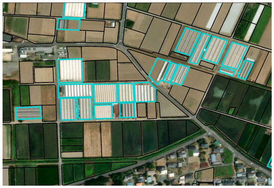
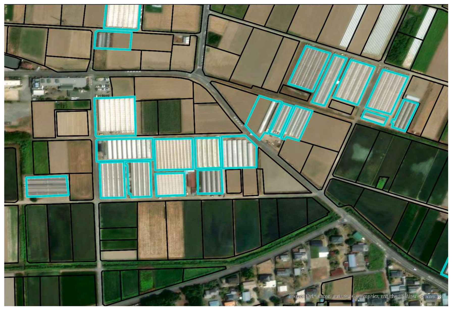
Prior to the quantitative accuracy evaluation, to qualitatively verify the detection performance in actual geographic space, the prediction results for the polygons in the study area were mapped onto the satellite imagery. Figure 5 shows the extraction results from the time-series RF model, which demonstrated the highest accuracy among the models constructed in this study. The polygons outlined in light blue in the figure represent the parcels predicted by the model as “with greenhouse.” Throughout the image, it was visually confirmed that greenhouses were appropriately extracted along the agricultural parcels without being influenced by their spatial arrangement or surrounding land uses (upland fields, paddy fields, and urban areas). This included extractions ranging from areas where greenhouses are densely concentrated, to isolated greenhouses within typical agricultural land, and further to small-scale greenhouses only partially contained within a polygon.

Figure 5. Detection results of plastic-covered greenhouses using the Random Forest model with time-series data. The polygons outlined in light blue in the figure represent the parcels predicted by the model as “with greenhouse”.

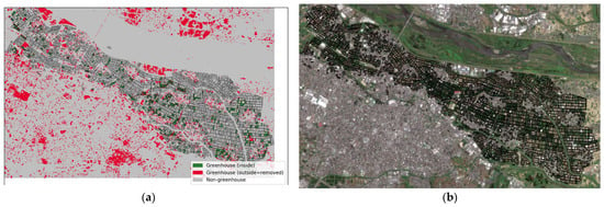
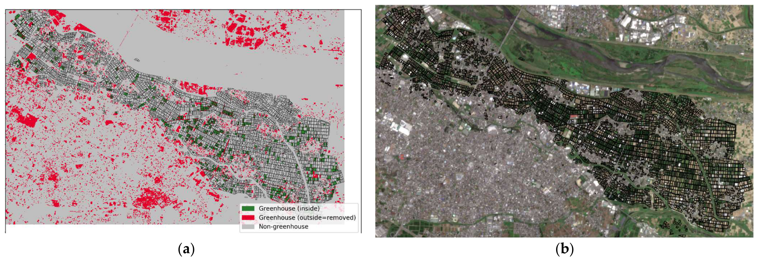
As a result of the ablation experiment, when no masking with the agricultural polygons was applied, 81.9% (381.5 ha) of the pixels predicted as greenhouse (465.9 ha in total) were distributed outside the agricultural polygons (Figure 6 and Table 3). In contrast, the greenhouse predictions remaining after masking (84.4 ha) were confined entirely within the agricultural parcels. Thus, the pre-masking step structurally removes false detections that do not originate from agricultural land, and thereby contributes to efficient greenhouse detection.

Figure 6. Ablation of the pre-masking step (within the polygon bounding box): (a) whole-scene pixel-wise greenhouse prediction by the time-series RF model (green: inside agricultural polygons; red: outside polygons, i.e., false detections structurally removed by pre-masking); (b) the corresponding true-color satellite image of the same extent.

Table 3. Ablation of the pre-masking step, evaluated within the polygon bounding box.

Category	Pixels	Area (ha)	Proportion (%)
Predicted greenhouse (whole scene, no masking)	517,607	465.9	100
Inside agricultural polygons	93,733	84.4	18.1
Outside polygons (removed by pre-masking)	423,874	381.5	81.9

3.2. Accuracy Comparison of Each Classification Model

Table 4 shows the accuracy comparison results for greenhouse detection based on differences in the machine learning algorithms (RF, SVM, and ISF) and the dimensionality of the input data (Single-Image: 6 dimensions, Time-Series Image: 24 dimensions).

Table 4. Performance evaluation results for greenhouse detection across different models. All metrics are computed at the polygon level; the pixel-level OA values are given in the text of Section 3.2.

Model	Features	Precision	Recall	F1-Score	OA	Optimal Threshold
Random Forest	Time-series (24 dimensions)	0.91	0.81	0.86	0.97	31%
Random Forest	Single-date (6 dimensions)	0.87	0.86	0.86	0.97	32%
Support Vector Machine	Time-series (24 dimensions)	0.84	0.87	0.86	0.96	39%
Support Vector Machine	Single-date (6 dimensions)	0.89	0.83	0.86	0.97	47%
Isolation Forest	Time-series (24 dimensions)	0.75	0.69	0.72	0.93	14%

In the evaluation on the test data, the F1-score for the greenhouse class was approximately 0.86 and essentially equivalent for both RF and SVM and for both the time-series and single-image datasets. The SVM, to which feature standardization and hyperparameter optimization had been applied, also reached a peak performance equivalent to that of RF. Accordingly, there is no significant difference among the methods in terms of the polygon-level F1-score, and in practical operation the robustness to the decision threshold, discussed below, becomes the deciding factor in the choice of method. The pixel-level OA was 0.89 for RF with time-series data, 0.87 for SVM with time-series data, 0.85 for RF with single-image data, and 0.82 for SVM with single-image data. As a representative example, the confusion matrix of the recommended method, RF with time-series data, is shown in Table 5.

Table 5. Confusion matrix for greenhouse detection using the time-series Random Forest model.

	Predicted: Non-Greenhouse (Field/Paddy)	Predicted: Greenhouse (Full/Partial)	Total
Actual: Non-greenhouse (Field/Paddy)	866	10	876
Actual: Greenhouse (Full/Partial)	24	103	127
Total	890	113	1003

The actual prediction results for the “with greenhouse” (greenhouse/partial greenhouse) class showed 103 correct detections (True Positives), 24 missed detections (False Negatives), and 10 false detections (False Positives) (Table 5). Despite the dataset being imbalanced, with greenhouse polygons accounting for approximately 13% of the 1003 test polygons, the model achieved a precision of 0.91, a recall of 0.81 and an F1-score of 0.86. The polygon-level OA was 0.97.

3.3. Sensitivity Analysis of the Polygon-Level Decision Threshold

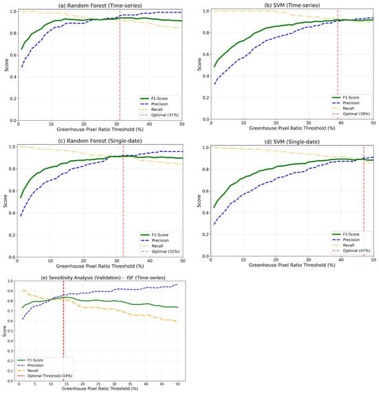
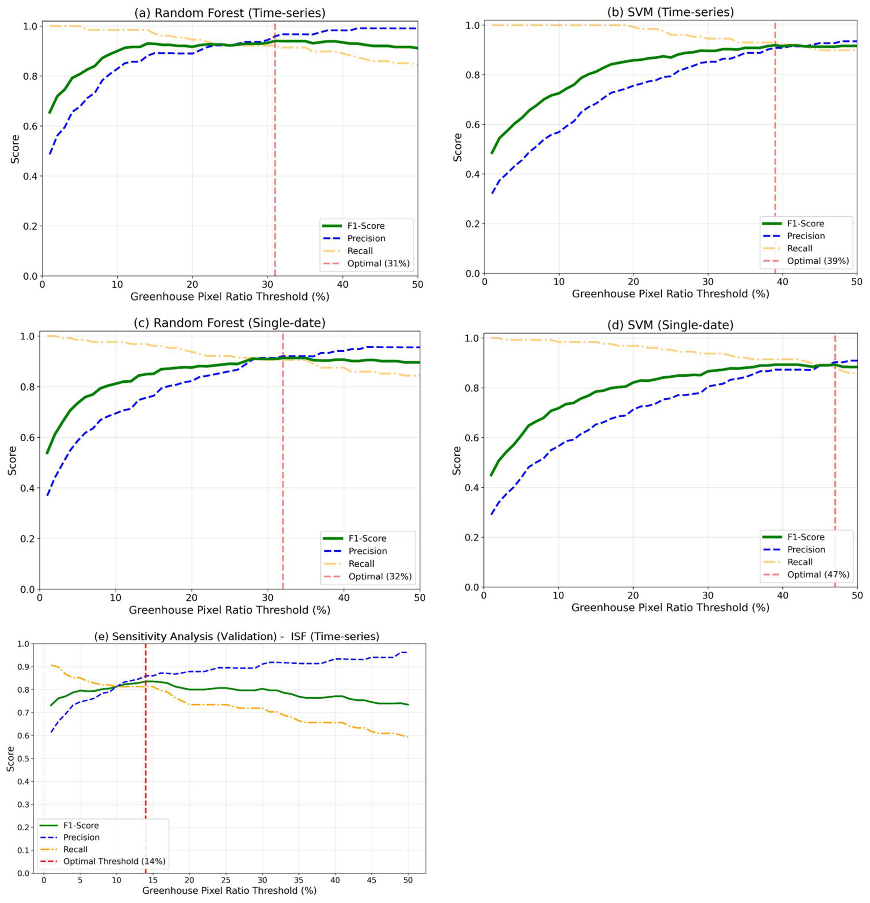
The results of the sensitivity analysis of the polygon-level decision threshold on precision, recall, and F1-score using the validation data are shown in Figure 7.The optimal threshold determined for each model, and the validation F1-score at that threshold, were 31% and 0.940 for RF with time-series data, 32% and 0.913 for RF with single-image data, 39% and 0.919 for SVM with time-series data, 47% and 0.893 for SVM with single-image data, and 14% and 0.835 for ISF with time-series data. What is important is that while the final peak performance is similar for RF and SVM, their robustness to the threshold differs markedly. RF with time-series data maintained a plateau with an F1-score of around 0.90 even when the threshold on the proportion of greenhouse pixels was varied over a wide range above approximately 10% and was therefore robust to the threshold setting. By contrast, SVM with time-series data showed a large decrease in the F1-score at low thresholds (for example, approximately 0.49 at a threshold of 1%) and only reached a level comparable to RF near its optimum of around 40%.

Figure 7. Sensitivity analysis of the polygon-level decision threshold for each model: (a) Random Forest (time-series); (b) SVM (time-series); (c) Random Forest (single-date); (d) SVM (single-date); (e) Isolation Forest (time-series). The red dashed line indicates the optimal threshold.

3.4. Evaluation of Feature Importance

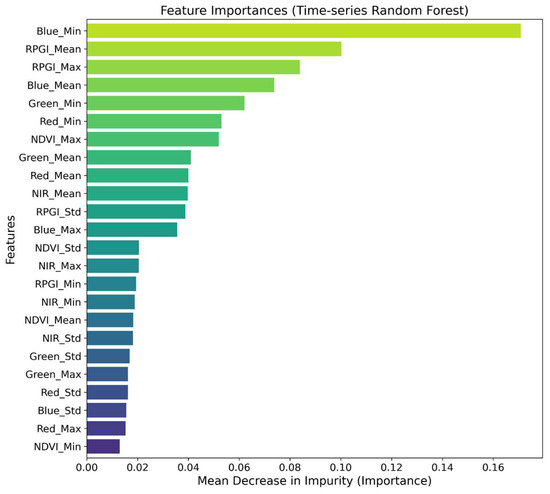
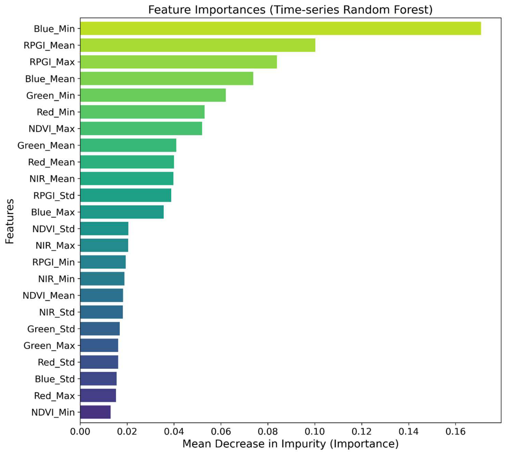
Figure 8 shows the contribution (importance) of each feature in the RF time-series model, which achieved the best performance.

Figure 8. Feature importance evaluated by the Random Forest model.

Examining the top features, Blue_Min exhibited the highest importance, followed by RPGI_Mean, RPGI_Max, and Blue_Mean. That is, the reflectance statistics of the Blue band (Blue_Min and Blue_Mean) and the statistics (mean and maximum) of the RPGI (plastic index), which was introduced to capture the optical reflectance characteristics of artificial structures, occupied the highest ranks. These results quantitatively demonstrate that they are effective indicators for discriminating plastic greenhouses (covering materials) from typical agricultural land (vegetation and soil).

4. Discussion

4.1. Causes of False Detections (False Positives) and Limitations of Spatial Resolution

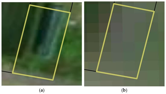
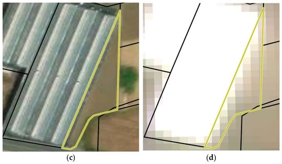
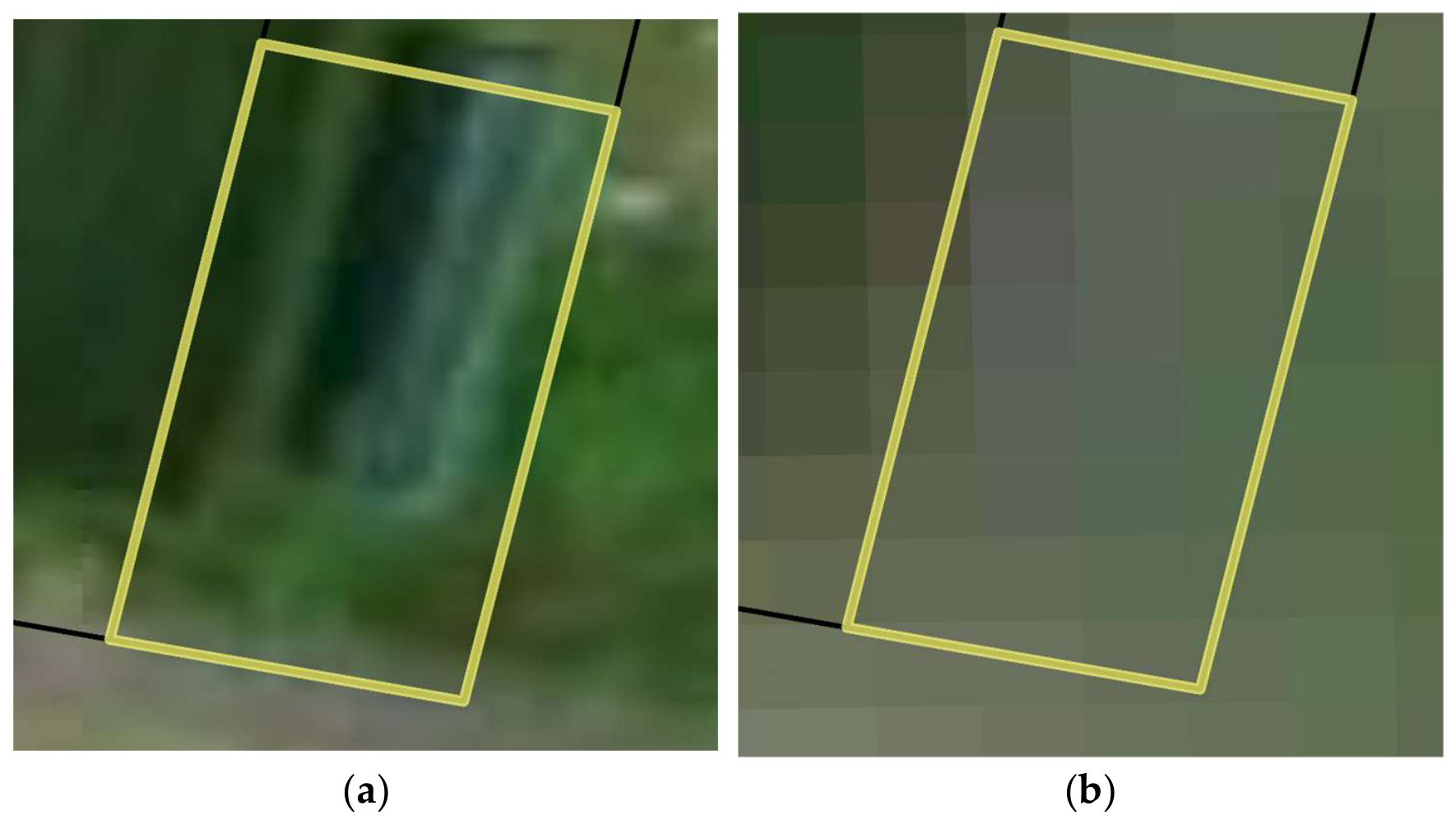
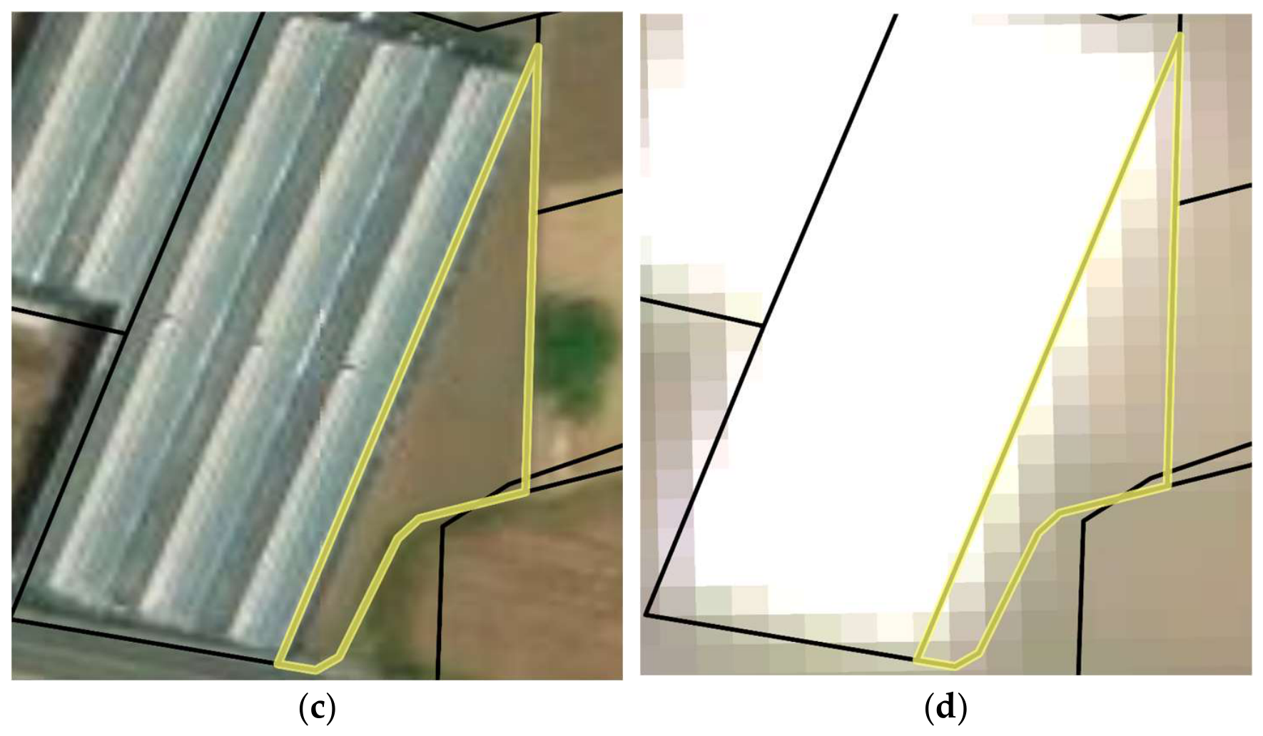
Although the model constructed in this study demonstrated high overall detection accuracy (F1-score: 0.86) and achieved favorable results in wide-area mapping, misclassifications occurred in some parcels. Figure 9 shows representative enlarged views of the misclassified polygons. The yellow outlines in the figure represent the target agricultural polygons, where (a) and (c) are the high-resolution images (WorldView-3, captured on 22 November 2024) utilized as ground truth, and (b) and (d) are the corresponding PlanetScope images.

Figure 9. Examples of misclassified polygons (indicated by yellow outlines): (a) ground truth image (WorldView-3, acquired on 22 November 2024) showing an existing greenhouse; (b) corresponding PlanetScope image where the greenhouse was undetected (false negative) due to the influence of surrounding vegetation; (c) ground truth image (WorldView-3, acquired on 22 November 2024) showing no greenhouse; (d) corresponding PlanetScope image where the polygon was falsely detected as a greenhouse (false positive) due to mixed pixels at the boundary with an adjacent greenhouse.

The first case is the missed detection (false negative) of greenhouses due to the influence of the surrounding environment. In the high-resolution image of Figure 9a, a greenhouse can be clearly confirmed within the polygon; however, in the PlanetScope image of Figure 9b, due to the constraint of spatial resolution (approximately 3 m), it was affected by the surrounding vegetation and other factors. As a result, the features at the pixel level were not sufficiently extracted as a greenhouse, resulting in a missed detection (False Negative). It has been pointed out that the accuracy of object extraction in agricultural environments depends on spatial resolution, and when the resolution is not sufficiently high relative to the size of the object, attenuation of spectral characteristics occurs due to mixels (mixed pixels) [24]. It is considered that this case was also affected by this phenomenon.

The second case is the false detection (false positive) caused by mixels at the boundaries. As Figure 9c shows, there is essentially no facility within the target polygon. However, when observing the PlanetScope image in Figure 9d, the pixels of a plastic greenhouse present in an adjacent parcel slightly interfere with the target polygon. For pixels located on the boundary of agricultural parcels, the reflectance characteristics of the ground surface (soil and vegetation) within the target polygon and the reflectance characteristics of the adjacent plastic greenhouse are recorded as a mixture. Consequently, even in areas where greenhouses are essentially absent, the RPGI and other metrics of the pixels near the boundary were calculated to be high, which likely led the model to determine them as greenhouse pixels. Because the decision threshold in this study was determined by a sensitivity analysis (31% for RF with time-series data), it is presumed that for polygons with a small area or an elongated shape, these boundary mixels alone exceeded the optimal threshold, resulting in the entire polygon being falsely detected as “with greenhouse.” It has been reported that spectral variations within an object and boundary disturbances in high-resolution images are factors that complicate classification [8]. Based on this, it is considered that in this case as well, the mixing of spectral characteristics (mixels) in the boundary region between different adjacent features acted as an error factor in small-scale object extraction.

4.2. Factor Analysis of Performance Differences Among Classification Algorithms

In this study, RF and SVM showed essentially equivalent F1-scores of approximately 0.86 on the test data. Through feature standardization and hyperparameter optimization, the SVM (RBF kernel) achieved a peak performance equivalent to that of RF even in discriminating between classes with similar spectra, such as upland fields and bare land. In contrast to the report of Gungor et al. [33], who found RF to be superior, the peak performance of the two methods was equivalent in this study, and the practical difference between them lies in the robustness to the decision threshold discussed below.

Despite their similar peak performance, the two methods behave very differently with respect to the decision threshold (sensitivity analysis, Figure 7). RF remained stable with an F1-score of around 0.90 even when the threshold on the proportion of greenhouse pixels was varied widely from approximately 10% to 50%, whereas SVM showed a large decrease in the F1-score in the low-threshold range and matched RF only near its optimum of around 40%. This is considered to be because RF yields predictions with a clearly separated confidence distribution through the hierarchy of thresholds in its decision trees, whereas SVM predictions with low confidence tend to concentrate near the decision boundary. In view of deployment to unknown regions where the decision threshold cannot be optimized in advance, this robustness provides a practical basis for selecting RF as the first choice. Pelletier et al. [34] have also shown that RF gives stable, high accuracy in wide-area land cover classification using high-resolution satellite image time series, which is consistent with the robustness of RF observed in this study.

Turning to the ISF, the semi-supervised anomaly detection approach did not achieve sufficient accuracy (F1-score: 0.72). It appears that the significant diversity of the “normal data (upland fields and paddy fields)” in the study area had an impact. ISF is based on the premise that a small number of anomalies (greenhouses) exist at a distance from densely packed clusters of normal values. However, in actual agricultural fields, the reflectance characteristics of normal data themselves vary considerably throughout the year depending on crop types, growth stages, soil moisture content, and other factors. Consequently, it is suggested that a clear separation between anomalies and normal data was difficult. This is because the normal data contained much noise that could easily be considered “anomalous” (e.g., soil with high reflectance), and conversely, greenhouses with reduced reflectance due to dirt accumulation were buried within the distribution of normal data. In environments where the diversity of the normal data is large, the introduction of deep-learning-based anomaly detection [35] may improve the separation performance, and this remains a subject for future study.

4.3. Inference on Factors Contributing to Classification

Regarding the feature importance in the time-series RF model of this study (Figure 8), Blue_Min, RPGI_Mean, and RPGI_Max ranked at the top, and it was confirmed that they contributed to the model’s classification. As described in Section 2.4, the original RPGI proposed by Yang et al. [27] uses “Blue, Green, and Near-Infrared” for the average reflectance in the denominator; however, in this study, in accordance with a subsequent study [28], a formula using “Red, Green, and Near-Infrared” in the denominator was adopted. Despite using a different calculation formula from the original, the following factors based on the optical characteristics of the land surface can be inferred as the reasons why this index demonstrated effective classification performance.

That is, the maximization of the optical contrast between vegetation (open-field crops) and plastic greenhouses. Because the Red band functions as the main absorption band for photosynthesis by plant chlorophyll [26], the reflectance decreases in open-field crops where plants are actively growing. On the other hand, the plastic covering materials of greenhouses maintain a relatively high reflectance across the entire visible light spectrum. Therefore, by incorporating the Red band into the calculation of the denominator’s mean reflectance term, the term becomes smaller for pixels of open-field crops (vegetation), and the denominator becomes larger, resulting in the overall RPGI value being kept low. Conversely, for greenhouse pixels, the RPGI value is amplified. It is highly likely that incorporating this “absorption characteristic of vegetation in the Red band” into the formula highlighted the difference between plastics and surrounding agricultural land, functioning as an effective splitting criterion in the RF model.

Furthermore, the fact that seasonal statistics extracted from time-series data, such as the maximum (Max) and mean (Mean) of indices, consistently yield higher accuracy in greenhouse classification than single-image indices has been demonstrated in a comparative study by Aguilar et al. [36] covering multiple agricultural regions worldwide (Spain, Morocco, Italy, and Turkey). This serves as objective corroboration for the result that RPGI_Mean and RPGI_Max showed high importance in this study. The effectiveness of the modified RPGI is also consistent with the findings of the comprehensive comparison of spectral indices for Sentinel-2 [17] and of the modified index designed for fragmented terrains [18]. In addition, the high consistency observed between simultaneously acquired Sentinel-2 and Landsat 8 imagery over PCGs [37] and the annual mapping of greenhouses from long-term Landsat time series [20] support the validity of the present approach based on time-series statistics.

In addition, it is also important that the reflectance statistics of the Blue band (such as Blue_Min and Blue_Mean) ranked high in Figure 8. While plastic materials have a relatively high reflectance across the entire visible light spectrum, soil and many types of vegetation have the characteristic of low reflectance (or absorption) in the blue band. Therefore, it is considered that even the Blue band alone created a clear contrast between the surrounding open-field crops or dark soil and the bright plastic greenhouses, functioning as an effective indicator when the RF model identified greenhouses. This inference is consistent with the results reported in the study by Yang et al. [27], who proposed the RPGI, stating that the reflectance of the Blue band increases as the area ratio of greenhouses within a pixel increases (i.e., the blue wavelength reflectance of greenhouses is higher than that of vegetation and soil).

4.4. Novelty and Superiority of the Proposed Method Based on Comparison with Existing Methods

The extraction method constructed in this study achieved high accuracy (F1-score: 0.86) in the small-scale and complex agricultural landscapes characteristic of peri-urban areas. It is considered that the novelty of this method and its superiority over existing methods, which led to this result, can be summarized in the following two main points.

The first novel aspect is the spatial pre-constraining (masking) of the extraction targets using existing geographic information system (GIS) data (agricultural parcel polygons) maintained by the government. The pixel-based and object-based classification methods proposed to date [6,7] have primarily taken an approach of attempting to extract greenhouses directly from the entire image, relying solely on the spectral and spatial information obtained from satellite imagery. However, in peri-urban agriculture, non-agricultural artificial structures with reflectance characteristics similar to those of greenhouses (e.g., factories and metal roofs) are complexly mixed; therefore, it has been challenging to separate them [5].

By integrating existing agricultural land maps to pre-exclude non-agricultural areas from the analysis target, this study structurally eliminated “false detections derived from non-agricultural artificial structures,” which was a major error factor in peri-urban landscapes. This point is an advantage not found in conventional methods. In the ablation experiment presented in Section 3.1, when no masking was applied, 81.9% of the pixels predicted as greenhouse were distributed outside the agricultural polygons; that is, on non-agricultural surfaces such as buildings, urban areas, bare ground, and forest (Figure 6 and Table 3). It is known that such false detections readily occur in peri-urban areas where non-agricultural artificial structures with reflectance characteristics similar to those of greenhouses are intermingled [5]. The effectiveness of incorporating prior knowledge of the target area before classification has also been demonstrated in earlier work [14], and the present result quantitatively confirms that pre-masking contributes decisively to eliminating false detections originating from non-agricultural land.

The second novel aspect is the utilization of satellite data (PlanetScope) that combines high spatial resolution and high-frequency observation, incorporating year-round phenology (seasonal variations) into the machine learning model as statistics. In peri-urban environments where complex land uses are mixed, the combination of PlanetScope’s high spatial resolution of approximately 3 m and machine learning is an effective approach for achieving high-accuracy classification, which is difficult with medium-resolution imagery, as shown in the study by Lefulebe et al. [38]. By capturing the shapes of parcels in detail at a 3 m resolution and using the variations in reflectance and indices throughout the year (mean, maximum, minimum, standard deviation, etc.) as features, this method successfully distinguished “greenhouses with consistently high reflectance characteristics throughout the year” from “open-field crops whose conditions change seasonally” based on temporal variation patterns.

In this way, it can be concluded that the approach integrating the “spatial limitation of the analysis scope using existing data” and the “temporal (phenological) feature extraction using high-resolution, high-frequency time-series data” was an effective method for small-scale, dispersed agricultural lands in Japan. Indeed, studies across a variety of regions and methods are accumulating, including the mapping of protected agriculture in Mexico using cloud geoprocessing on Google Earth Engine [39], the pixel- and object-based comparison of Sentinel-2 and Landsat-8 data in Morocco [40], and the analysis of spatiotemporal changes in greenhouses by deep learning [41]. Unlike these approaches, which extract greenhouses from the entire image, the present study is novel in that it constrains the target in advance using existing agricultural polygons.

4.5. Limitations and Future Prospects of the Proposed Method

The method constructed in this study, which combines the time-series RF model with masking based on agricultural polygons, demonstrated favorable accuracy in the northern part of Honjo City, where flat agricultural land extends. However, several limitations remain for wide-area application and continuous monitoring in real-world environments.

First is the verification of generalizability to other regions and environments. Although the northern part of Honjo City has a relatively flat topography, if this method is applied to steep hilly and mountainous areas, there is a concern that the high reflectance characteristics specific to greenhouses may become difficult to capture due to the influence of topographic shadows (such as mountain shadows), potentially decreasing extraction accuracy. As a future prospect, it is necessary to extend the verification scope to municipalities with different topographical features and climatic conditions to evaluate the spatial generalization performance of the model. Veettil and Acharki [42] have quantitatively shown that elevation and terrain affect greenhouse mapping accuracy, so a decrease in accuracy should be borne in mind when the method is applied to mountainous or highland areas. Verification in regions with different topographic conditions is required, including areas where an expansion of PCGs at high elevations has been reported [43].

Second is the difficulty in detecting greenhouses that were installed or removed during the middle of the year, which stems from the characteristics of time-series analysis. Because the method in this study utilizes year-round statistics (such as mean and standard deviation) of reflectance and indices as features, for facilities newly established or removed mid-year, the year-round feature values become intermediate. Consequently, it is considered that model discrimination becomes more difficult compared to greenhouses that exist throughout the year, potentially leading to missed detections. As a future approach to this limitation, rather than relying on year-round statistics, introducing a dynamic analysis method that captures time-series changes over shorter periods, such as monthly or quarterly intervals, is expected to enable more detailed monitoring that includes not only the distribution of agricultural greenhouses but also the timing of their establishment and removal.

Third is the dependence on the development and public availability of “agricultural parcel polygon data,” which forms the foundation of this method. Within Japan, because MAFF maintains the “agricultural polygons” covering agricultural parcels nationwide as open data, this method is highly practical. Looking abroad, while member states of the European Union (EU) have meticulously constructed the Land Parcel Identification System (LPIS) based on the Common Agricultural Policy (CAP), in the United States, although the Common Land Unit (CLU) by the Department of Agriculture (USDA) exists, its public disclosure is strictly restricted from the perspective of privacy protection, resulting in significant variations in data availability depending on the region. Particularly in many emerging and developing countries, the development of wide-area and high-precision agricultural GIS data by governments has not progressed significantly, presenting a constraint where the masking process—a major strength of this method—cannot be directly applied. For expansion into areas where such existing open polygon data do not exist or where access is restricted, it is considered that the generalizability of the proposed method could be enhanced by utilizing deep learning or other techniques to automatically extract agricultural parcel boundaries from satellite imagery and applying the classification model of this study based on the extracted pseudo-polygons. In regions where existing polygons are not available, pseudo-polygons could be generated using deep learning for the automatic extraction of field boundaries from satellite imagery [44] or agglomerative segmentation for parcel delineation [45], and applying the present method to them would enhance its generalizability.

5. Conclusions

In this study, a method was developed to automatically and accurately extract agricultural greenhouses (PCGs) within the peri-urban agricultural landscapes of Japan, which are characterized by a complex mixture of small-scale and diverse land uses. To address the challenge of confusion with non-agricultural lands (such as buildings and other artificial structures) faced by conventional methods, this study proposed and verified a novel approach that integrates the spatial pre-constraining (masking) of analysis targets using existing administrative GIS data (agricultural polygons) with the utilization of year-round time-series phenology derived from PlanetScope satellite imagery (spatial resolution of approximately 3 m).

As a result of comparatively evaluating three types of machine learning algorithms, RF and SVM were able to extract greenhouses with essentially equivalent F1-scores of approximately 0.86. It was confirmed that the RF model effectively learned seasonal statistics (such as the mean and maximum values) of metrics like the modified RPGI (plastic index) and appropriately distinguished the differences between the unique reflectance characteristics of plastic materials and the vegetation phenology of crops. Although the peak performance of the two methods was equivalent, RF was robust to the decision threshold and was therefore practically advantageous for deployment to unknown regions where the threshold is difficult to optimize in advance. For ISF, challenges remained in improving classification accuracy due to the diversity of data distributions associated with seasonal variations and the overlap of spectral characteristics between classes. Furthermore, it was revealed that even when using high-resolution imagery, mixels (mixed pixels) occurring in the boundary regions with adjacent parcels decrease extraction accuracy.

The method proposed in this study serves as a practical framework for significantly reducing the costs of manual field surveys and automatically and accurately integrating the wide-area distribution of agricultural facilities into existing agricultural land maps (agricultural polygons). It is expected that the outcomes of this study will contribute as a useful decision support tool for infrastructure management and the formulation of sustainable agricultural plans in peri-urban agriculture.

References

- Veettil, B.K.; Van, D.D.; Quang, N.X.; Hoai, P.N. Remote sensing of plastic-covered greenhouses and plastic-mulched farmlands: Current trends and future perspectives. Land Degrad. Dev. 2023, 34, 591–609. [Google Scholar] [CrossRef] [Scilit]
- Picuno, P. Innovative Material and Improved Technical Design for a Sustainable Exploitation of Agricultural Plastic Film. Polym. Plast. Technol. Eng. 2014, 53, 1000–1011. [Google Scholar] [CrossRef] [Scilit]
- Ou, C.; Wang, Y. Tracking Spatio-Temporal Dynamics of Greenhouse-Led Cultivated Land and its Drivers in Shandong Province, China. Front. Environ. Sci. 2022, 10, 944422. [Google Scholar] [CrossRef] [Scilit]
- Niu, B.; Feng, Q.; Qiu, B.; Su, S.; Zhang, X.; Cui, R.; Zhang, X.; Sun, F.; Yan, W.; Zhao, S.; et al. Global-PCG-10: A 10 m global map of plastic-covered greenhouses derived from Sentinel-2 in 2020. Earth Syst. Sci. Data 2025, 17, 5065–5088. [Google Scholar] [CrossRef] [Scilit]
- Levin, N.; Lugassi, R.; Ramon, U.; Braun, O.; Ben-Dor, E. Remote sensing as a tool for monitoring plasticulture in agricultural landscapes. Int. J. Remote Sens. 2007, 28, 183–202. [Google Scholar] [CrossRef] [Scilit]
- Lu, L.; Di, L.; Ye, Y. A decision-tree classifier for extracting transparent plastic-mulched landcover from Landsat-5 TM images. IEEE J. Sel. Top. Appl. Earth Obs. Remote Sens. 2014, 7, 4548–4558. [Google Scholar] [CrossRef] [Scilit]
- Wang, C.; Lu, L. Object-based random forest classification for detecting plastic-mulched landcover from Gaofen-2 and Landsat-8 OLI fused data. In Proceedings of the 8th International Conference on Agro-Geoinformatics, Istanbul, Turkey, 16–19 July 2019. [Google Scholar]
- Agüera, F.; Aguilar, M.A.; Aguilar, F.J. Detecting greenhouse changes from QuickBird imagery on the Mediterranean coast. Int. J. Remote Sens. 2006, 27, 4751–4767. [Google Scholar] [CrossRef] [Scilit]
- Aguilar, M.A.; Nemmaoui, A.; Novelli, A.; Aguilar, F.J.; Lorca, A.G. Object-based greenhouse mapping using very high resolution satellite data and Landsat-8 time series. Remote Sens. 2016, 8, 513. [Google Scholar] [CrossRef] [Scilit]
- Balcik, F.B.; Senel, G.; Goksel, C. Object-Based Classification of Greenhouses Using Sentinel-2 MSI and SPOT-7 Images: A Case Study from Anamur (Mersin), Turkey. IEEE J. Sel. Top. Appl. Earth Obs. Remote Sens. 2020, 13, 2769–2777. [Google Scholar] [CrossRef] [Scilit]
- Peña, J.M.; Gutiérrez, P.A.; Hervás-Martínez, C.; Six, J.; Plant, R.E.; López-Granados, F. Object-Based Image Classification of Summer Crops with Machine Learning Methods. Remote Sens. 2014, 6, 5019–5041. [Google Scholar] [CrossRef] [Scilit]
- Chen, W.; Xu, Y.; Zhang, Z.; Yang, L.; Pan, X.; Jia, Z. Mapping agricultural plastic greenhouses using Google Earth images and deep learning. Comput. Electron. Agric. 2021, 191, 106552. [Google Scholar] [CrossRef] [Scilit]
- Chen, W.; Li, J.; Wang, D.; Xu, Y.; Liao, X.; Wang, Q.; Chen, Z. Large-scale automatic extraction of agricultural greenhouses based on high-resolution remote sensing and deep learning technologies. Environ. Sci. Pollut. Res. 2023, 30, 106671–106686. [Google Scholar] [CrossRef] [Scilit] [PubMed]
- Zhou, C.; Huang, J.; Xiao, Y.; Du, M.; Li, S. A novel approach: Coupling prior knowledge and deep learning methods for large-scale plastic greenhouse extraction using Sentinel-1/2 data. Int. J. Appl. Earth Obs. Geoinf. 2024, 132, 104073. [Google Scholar] [CrossRef] [Scilit]
- Hong, R.; Xiao, B.; Yan, H.; Liu, J.; Liu, P.; Song, Z. Multitemporal greenhouse mapping for high-resolution remote sensing imagery based on an improved YOLOX. Comput. Electron. Agric. 2023, 206, 107689. [Google Scholar] [CrossRef] [Scilit]
- Sun, H.; Wang, L.; Lin, R.; Zhang, Z.; Zhang, B. Mapping Plastic Greenhouses with Two-Temporal Sentinel-2 Images and 1D-CNN Deep Learning. Remote Sens. 2021, 13, 2820. [Google Scholar] [CrossRef] [Scilit]
- Senel, G.; Aguilar, M.A.; Aguilar, F.J.; Nemmaoui, A.; Goksel, C. A Comprehensive Benchmarking of the Available Spectral Indices Based on Sentinel-2 for Large-Scale Mapping of Plastic-Covered Greenhouses. IEEE J. Sel. Top. Appl. Earth Obs. Remote Sens. 2023, 16, 6601–6613. [Google Scholar] [CrossRef] [Scilit]
- Chen, S.; Chen, Y.; Gao, S.; Li, C.; Li, N.; Chen, L. A modified spectral remote sensing index to map plastic greenhouses in fragmented terrains. Smart Agric. Technol. 2025, 11, 100904. [Google Scholar] [CrossRef] [Scilit]
- Lin, J.; Jin, X.; Ren, J.; Liu, J.; Liang, X.; Zhou, Y. Rapid Mapping of Large-Scale Greenhouse Based on Integrated Learning Algorithm and Google Earth Engine. Remote Sens. 2021, 13, 1245. [Google Scholar] [CrossRef] [Scilit]
- Ou, C.; Yang, J.; Du, Z.; Zhang, T.; Niu, B.; Feng, Q.; Liu, Y.; Zhu, D. Landsat-Derived Annual Maps of Agricultural Greenhouse in Shandong Province, China from 1989 to 2018. Remote Sens. 2021, 13, 4830. [Google Scholar] [CrossRef] [Scilit]
- Ibrahim, E.; Gobin, A. Sentinel-2 Recognition of Uncovered and Plastic Covered Agricultural Soil. Remote Sens. 2021, 13, 4195. [Google Scholar] [CrossRef] [Scilit]
- de Souza, M.F.; Lamparelli, R.A.C.; Oliveira, M.H.S.; Nogueira, G.P.; Bliska, A., Jr.; Franco, T.T. Remote sensing detection of plastic-mulched farmland using a temporal approach in machine learning: Case study in tomato crops. Environ. Sci. Pollut. Res. 2024, 32, 31222–31235. [Google Scholar] [CrossRef] [Scilit] [PubMed]
- Houborg, R.; McCabe, M.F. A Cubesat enabled Spatio-Temporal Enhancement Method (CESTEM) utilizing Planet, Landsat and MODIS data. Remote Sens. Environ. 2018, 209, 211–226. [Google Scholar] [CrossRef] [Scilit]
- Cui, B.; Huang, W.; Ye, H.; Chen, Q.; Li, Z.; Jiang, H. Optimal spatial resolution of remote-sensing imagery for monitoring cantaloupe greenhouses. IOP Conf. Ser. Earth Environ. Sci. 2022, 1004, 012020. [Google Scholar] [CrossRef] [Scilit]
- Johansen, K.; Ziliani, M.G.; Houborg, R.; Franz, T.E.; McCabe, M.F. CubeSat constellations provide enhanced crop phenology and digital agricultural insights using daily leaf area index retrievals. Sci. Rep. 2022, 12, 5244. [Google Scholar] [CrossRef] [Scilit] [PubMed]
- Tucker, C.J. Red and photographic infrared linear combinations for monitoring vegetation. Remote Sens. Environ. 1979, 8, 127–150. [Google Scholar] [CrossRef] [Scilit]
- Yang, D.; Chen, J.; Zhou, Y.; Chen, X.; Chen, X.; Cao, X. Mapping plastic greenhouse with medium spatial resolution satellite data: Development of a new spectral index. ISPRS J. Photogramm. Remote Sens. 2017, 128, 47–60. [Google Scholar] [CrossRef] [Scilit]
- Acharki, S.; Veettil, B.K. Mapping plastic-covered greenhouse farming areas using high-resolution PlanetScope and RapidEye imagery: Studies from Loukkos perimeter (Morocco) and Dalat City (Vietnam). Environ. Sci. Pollut. Res. 2023, 30, 23012–23022. [Google Scholar] [CrossRef] [Scilit] [PubMed]
- Breiman, L. Random forests. Mach. Learn. 2001, 45, 5–32. [Google Scholar] [CrossRef] [Scilit]
- Belgiu, M.; Drăguț, L. Random forest in remote sensing: A review of applications and future directions. ISPRS J. Photogramm. Remote Sens. 2016, 114, 24–31. [Google Scholar] [CrossRef] [Scilit]
- Mountrakis, G.; Im, J.; Ogole, C. Support vector machines in remote sensing: A review. ISPRS J. Photogramm. Remote Sens. 2011, 66, 247–259. [Google Scholar] [CrossRef] [Scilit]
- Liu, F.T.; Ting, K.M.; Zhou, Z.H. Isolation forest. In Proceedings of the 2008 Eighth IEEE International Conference on Data Mining, Pisa, Italy, 15–19 December 2008; pp. 413–422. [Google Scholar]
- Gungor, R.; Sanli, F.B.; Ates, A.M.; Yilmaz, O.S. Evaluation of Classification Accuracy of Spectral Indices and Machine Learning Algorithms for Greenhouse Detection Using the Google Earth Engine Platform. J. Agric. Sci. 2026, 32, 158–176. [Google Scholar] [CrossRef] [Scilit]
- Pelletier, C.; Valero, S.; Inglada, J.; Champion, N.; Dedieu, G. Assessing the robustness of Random Forests to map land cover with high resolution satellite image time series over large areas. Remote Sens. Environ. 2016, 187, 156–168. [Google Scholar] [CrossRef] [Scilit]
- Pang, G.; Shen, C.; Cao, L.; van den Hengel, A. Deep Learning for Anomaly Detection: A Review. ACM Comput. Surv. 2021, 54, 1–38. [Google Scholar] [CrossRef] [Scilit]
- Aguilar, M.A.; Jiménez-Lao, R.; Ladisa, C.; Aguilar, F.J.; Tarantino, E. Comparison of spectral indices extracted from Sentinel-2 images to map plastic covered greenhouses through an object-based approach. GIScience Remote Sens. 2022, 59, 822–842. [Google Scholar] [CrossRef] [Scilit]
- Aguilar, M.A.; Jiménez-Lao, R.; Nemmaoui, A.; Aguilar, F.J.; Koc-San, D.; Tarantino, E.; Chourak, M. Evaluation of the Consistency of Simultaneously Acquired Sentinel-2 and Landsat 8 Imagery on Plastic Covered Greenhouses. Remote Sens. 2020, 12, 2015. [Google Scholar] [CrossRef] [Scilit]
- Lefulebe, B.E.; Van der Walt, A.; Xulu, S. Fine-Scale Classification of Urban Land Use and Land Cover with PlanetScope Imagery and Machine Learning Strategies in the City of Cape Town, South Africa. Sustainability 2022, 14, 9139. [Google Scholar] [CrossRef] [Scilit]
- Perilla, G.A.; Mas, J.-F. High-resolution mapping of protected agriculture in Mexico, through remote sensing data cloud geoprocessing. Eur. J. Remote Sens. 2019, 52, 532–541. [Google Scholar] [CrossRef] [Scilit]
- Acharki, S.; Veettil, B.K.; Vizzari, M. Plastic-covered greenhouses mapping in Morocco with Google Earth Engine: Comparing Sentinel-2 and Landsat-8 data using pixel- and object-based methods. Remote Sens. Appl. Soc. Environ. 2024, 34, 101158. [Google Scholar] [CrossRef] [Scilit]
- Zheng, M.; Liu, L.; Wu, J.; Du, S. Spatiotemporal evolution of agricultural greenhouses based on remote sensing data: A case study of Weinan City in China. J. Agric. Food Res. 2025, 24, 102326. [Google Scholar] [CrossRef] [Scilit]
- Veettil, B.K.; Acharki, S. Influence of elevation on plastic-covered greenhouse mapping accuracy using high-resolution satellite imagery and machine learning algorithms. Remote Sens. Lett. 2023, 14, 413–422. [Google Scholar] [CrossRef] [Scilit]
- Veettil, B.K.; Xuan, Q.N. Landsat-8 and Sentinel-2 data for mapping plastic-covered greenhouse farming areas: A study from Dalat City (Lam Dong Province), Vietnam. Environ. Sci. Pollut. Res. 2022, 29, 73926–73933. [Google Scholar] [CrossRef] [Scilit] [PubMed]
- Waldner, F.; Diakogiannis, F.I. Deep learning on edge: Extracting field boundaries from satellite images with a convolutional neural network. Remote Sens. Environ. 2020, 245, 111741. [Google Scholar] [CrossRef] [Scilit]
- García-Pedrero, A.; Gonzalo-Martín, C.; Lillo-Saavedra, M. A machine learning approach for agricultural parcel delineation through agglomerative segmentation. Int. J. Remote Sens. 2017, 38, 1809–1819. [Google Scholar] [CrossRef] [Scilit]
Disclaimer/Publisher’s Note: The statements, opinions and data contained in all publications are solely those of the individual author(s) and contributor(s) and not of MDPI and/or the editor(s). MDPI and/or the editor(s) disclaim responsibility for any injury to people or property resulting from any ideas, methods, instructions or products referred to in the content. |
© 2026 by the authors. Licensee MDPI, Basel, Switzerland. This article is an open access article distributed under the terms and conditions of the Creative Commons Attribution (CC BY) license.