


Abstract
Accurate prediction of coupled heat-transfer and fluid-flow phenomena is essential for the thermal design, performance assessment, and optimization of heat exchangers (HXs). Among key HXs, concentric tube heat exchangers (CTHXs) are widely used in thermal energy systems, where their performance is governed by the coupled interaction of fluid flow and heat transfer. Although computational fluid dynamics (CFD) provides detailed insights into these transport phenomena, its high computational cost limits its applicability in design optimization and real-time monitoring applications. To overcome this limitation, the present study proposes a physics-guided neural network (PGNN) for the accurate and efficient prediction of CTHX thermo-hydraulic performance, including the overall heat-transfer coefficient (U) and the pressure drops of the cold (ΔPc) and hot (ΔPh) streams. The PGNN introduces correlation-based physical guidance through established Nusselt number, overall thermal-resistance, and Darcy–Weisbach pressure-drop relations. Accordingly, the proposed framework is a correlation-guided PGNN rather than a residual-based physics-informed model, because the local conservation-equation residuals are not explicitly enforced during training. For comparison, a standard artificial neural network (ANN) with the same architecture and input parameters was also developed. Both models were trained on a dataset generated from 1575 CFD simulations covering a wide range of operating and geometric conditions, including the Reynolds and Prandtl numbers of both fluids, inner and outer tube diameters, and inlet temperatures. A comprehensive error analysis demonstrates the superior predictive capability of the PGNN over the ANN under various flow and geometric conditions. On the unseen test dataset, the PGNN achieved mean absolute percentage errors of 2.03%, 1.09%, and 1.11% for predicting U, ΔPc, and ΔPh, respectively. The proposed PGNN therefore provides a reliable, high-fidelity, and computationally efficient alternative to CFD, supporting the analysis, optimization, and operation of thermal energy systems.
1. Introduction
Heat exchangers (HXs) are critical devices designed to transfer thermal energy efficiently between two or more media, enabling key processes such as heating, cooling, and drying. They are widely employed across a range of industries, including thermal energy storage [1,2], sustainable heating [3], and evaporative cooling [4], where their performance directly affects the overall system’s energy efficiency. Among the various configurations, concentric tube heat exchangers (CTHXs) are widely used due to their compact geometry, straightforward construction, and high thermal effectiveness [5]. Their versatility in facilitating efficient heat transfer between different fluids, such as air and water, makes them particularly suitable for numerous industrial and engineering applications.
Accurate and high-fidelity evaluation of HX performance is crucial for enhancing operational efficiency and for optimizing design strategies [6,7,8,9,10,11,12]. Both thermal and hydraulic characteristics strongly influence the overall performance of HXs, and improving thermal performance often increases hydraulic losses [10]. Recent advances in computational methods have enabled detailed performance prediction through Computational Fluid Dynamics (CFD). CFD techniques solve the governing Navier–Stokes and energy equations to simulate conjugate heat transfer within heat exchangers, providing detailed insights into their thermal and hydraulic behavior. Nevertheless, achieving such high-resolution results typically requires significant computational time and resources.
Over recent years, data-driven surrogate models have gained prominence as an effective approach for simulating heat transfer and fluid flow in heat exchangers [13,14,15,16]. These models leverage machine learning techniques to approximate complex, nonlinear relationships between input parameters such as fluid properties, flow rates, and geometric features and output responses, such as heat-transfer coefficients, without relying on explicit analytical expressions. Artificial neural networks (ANNs) have been particularly successful in this context. For instance, Çolak et al. [17] employed an ANN to predict critical heat-transfer parameters in a shell-and-helically-coiled-tube heat exchanger, achieving an R2 coefficient of 0.998. Other machine learning methods, including random forest ensembles [11], have also been applied to estimate convective heat transfer and pressure drop, offering rapid predictions once the models are trained. When trained on high-fidelity simulation or experimental data, these surrogate models provide a computationally efficient alternative to conventional CFD simulations, enabling fast yet reliable performance evaluations [18].
Despite their advantages, purely data-driven approaches face significant limitations. First, they typically require large, high-quality datasets to achieve accurate predictions, making them “data-intensive.” Second, such models do not inherently incorporate the underlying physical laws, which can lead to unrealistic or non-physical results when applied outside the range of their training data [19]. In the case of HXs, generating sufficient training data is often challenging: experimental measurements are expensive and time-consuming, while high-fidelity CFD simulations demand substantial computational resources. Moreover, black-box models may violate fundamental principles such as energy conservation or flow continuity, when extrapolated beyond the regime covered by the training dataset. These challenges have motivated the development of hybrid modeling strategies that integrate data-driven flexibility with the enforcement of physical constraints, combining the strengths of both approaches.
Physics-guided neural networks (PGNNs) have recently emerged as a robust framework for surrogate modeling in heat-transfer and fluid-flow applications [20,21]. These models extend conventional deep learning approaches by embedding physical knowledge commonly represented by partial differential equations or empirical correlations into the training procedure as constraints [22]. This integration enables the model to respect fundamental physical principles, thereby reducing its reliance on extensive labeled datasets and enhancing its generalization. For instance, Abdulkarim et al. [20] developed two PGNNs to predict the Nusselt number and performance evaluation criterion (PEC) in shell-and-helical coil heat exchangers by incorporating empirical heat-transfer correlations into the loss function, demonstrating superior accuracy and robustness compared to conventional correlations and various machine learning models, achieving a high coefficient of determination R2 of 0.997. Bokil et al. [21] developed a geometry-adaptive, physics-informed convolutional neural network surrogate model to predict velocity, pressure, and temperature fields in HX tube bundles by embedding RANS equations and boundary conditions into the training process. Their approach achieved approximately 97% prediction accuracy on unseen geometries and outperformed purely data-driven models, demonstrating improved reliability while reducing the need for extensive CFD simulations. Liang et al. [23] developed a physics-informed deep residual network to predict the performance of finned-tube evaporators by integrating prior physical knowledge into the model architecture. Their model achieved high predictive accuracy, with mean absolute errors of 0.14% for heat-transfer rate, 0.36% for refrigerant pressure drop, and 0.49% for air pressure drop, outperforming conventional machine learning approaches in capturing detailed physical behavior. Moreover, Cai et al. [24] applied physics-informed neural networks to solve a range of heat-transfer problems, including convection and phase-change phenomena, using sparse and noisy data while enforcing governing physical laws. Their results demonstrated that PGNNs can accurately reconstruct temperature and velocity fields and address ill-posed problems beyond the capabilities of traditional computational methods. Majumdar et al. [25] introduced HxPINN, a hypernetwork-based physics-informed neural network for real-time monitoring of industrial heat exchangers under varying operating conditions. Their model achieved temperature prediction errors below 5 °C while accelerating inference by approximately 35–40 times compared to conventional physics-based approaches, demonstrating strong potential for digital twin applications. Shan et al. [26] proposed a physics-guided collaborative modeling (PGCM) framework for air source heat pump systems, integrating a heat exchanger physics-informed neural network (HX-PINN) with a system-level solver to capture nonlinear heat transfer and thermodynamic interactions. Their approach achieved a high predictive accuracy of 99.3% for pressure drop and 98.5% for enthalpy change while reducing computational time by up to 95.2% and maintaining a mean absolute COP (coefficient of performance) error of 1.5%. Collectively, these studies highlight the capability of PGNNs to act as accurate, physics-guided surrogate models for thermofluid systems, addressing the data scarcity and interpretability limitations commonly associated with purely empirical or black-box approaches.
The present work develops a physics-guided neural network (PGNN) framework for predicting the thermo-hydraulic performance of concentric tube heat exchangers (CTHXs) through the simultaneous estimation of the overall heat-transfer coefficient (U) and the pressure drops of the cold () and hot () streams. Although PGNNs have been successfully applied in various engineering disciplines, their application to the thermo-hydraulic modeling of CTHXs has received limited attention. The scientific contributions of this work are summarized as follows:
- Development of a PGNN specifically designed for the thermo-hydraulic modeling of CTHXs, enabling the simultaneous prediction of the overall heat-transfer coefficient and the pressure drops of both hot and cold streams.
- Integration of validated thermo-hydraulic empirical correlations into the training process as physics-based constraints, thereby enforcing physically consistent predictions while improving the model’s generalization capability.
- Systematic evaluation of the proposed PGNN against a conventional artificial neural network (ANN), demonstrating the advantages of physics-guided learning in terms of prediction accuracy and physical consistency.
- Demonstration that the proposed PGNN achieves high predictive accuracy on unseen test data, with mean absolute percentage errors of 2.03%, 1.09%, and 1.11% for U, , and , respectively, confirming its effectiveness for accurate and reliable thermo-hydraulic performance prediction of CTHXs.
The article is structured as follows: Section 2 presents the detailed methodology of CFD simulations, Section 3 describes the dataset preprocessing, Section 4 introduces the machine learning methodology including the ANN model and the proposed PGNN model, Section 5 provides a detailed error analysis to compare the predictive performance of the ANN and PGNN models, and Section 6 concludes with key findings and future perspectives.
2. Computational Fluid Dynamics (CFD)
2.1. Computational Domain
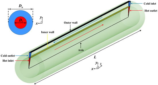
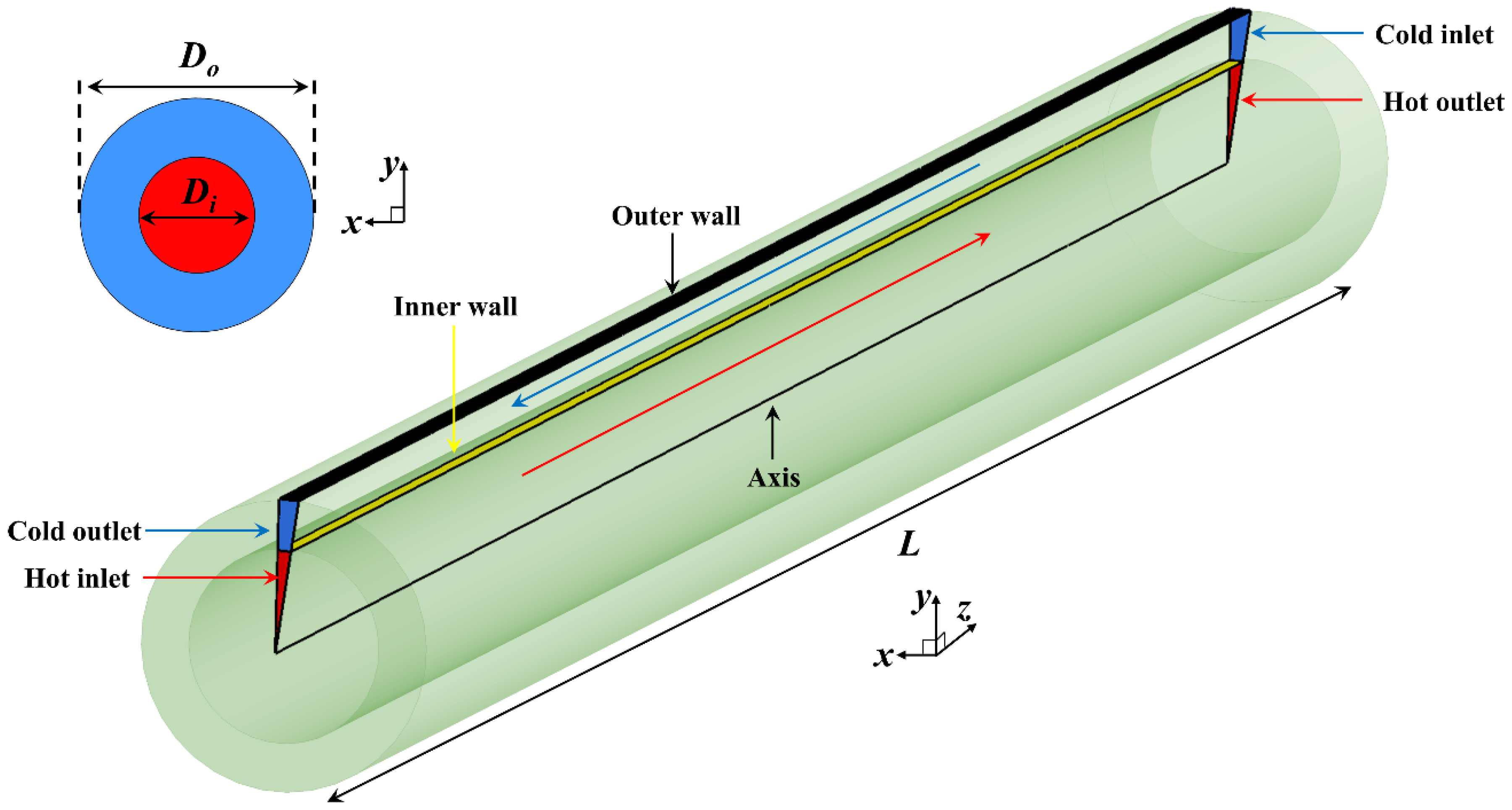
Figure 1 presents the layout of the counter-flow concentric tube heat-recovery exchanger (CTHX) considered in this study. The warm greywater stream flows through the central tube, while the cold-water stream passes through the annular space between the inner and outer walls. To reduce computational cost, the exchanger is modeled in a two-dimensional meridional plane under the axisymmetric assumption. This approach allows the selected section to reproduce the behavior of the complete three-dimensional device. The geometry is characterized mainly by the inner-tube diameter , the outer diameter , and the exchanger length .
Figure 1.
Computational domain of the CTHX.
A wide range of flow conditions is examined by considering inlet Reynolds numbers of 1000, 2000, 4000, 10,000, and 20,000. The cases at Reynolds numbers of 1000 and 2000 are classified as laminar, whereas those at Reynolds numbers of 4000, 10,000, and 20,000 are classified as turbulent. No cases are considered within the transitional range between the Reynolds numbers of 2300 and 4000. The temperature dependence of water properties is accounted for using a piecewise-linear interpolation based on the data reported by Bergman et al. [27]. The geometric parametric study includes three values of the inner diameter, namely 0.01, 0.02, and 0.05 m, combined with three diameter ratios equal to 1.25, 1.5, and 3. Four exchanger lengths are also investigated: 0.4, 0.6, 2, and 4 m.
To represent practical operating conditions, three inlet temperatures are imposed for each stream. The hot greywater enters at 365.15 K (92 °C), 338.15 K (65 °C), or 313.15 K (40 °C), whereas the cold-water inlet temperature is set to 298.15 K (25 °C), 288.15 K (15 °C), or 280.15 K (7 °C). The selected geometric and operating conditions were chosen to ensure that the investigated cases are representative of practical liquid-to-liquid CTHX applications. In particular, the Reynolds number ranges were selected to cover both laminar and turbulent-flow regimes, enabling the model to learn the thermo-hydraulic behavior over the operating conditions commonly encountered in industrial practice. Moreover, the selected hot- and cold-water temperature ranges are representative of typical liquid-to-liquid heat-transfer applications, thereby enhancing the practical relevance and applicability of the proposed PGNN framework.
The CFD dataset was generated using a deterministic reduced-factorial design rather than random sampling or Latin hypercube sampling. Although nine variables were subsequently provided as inputs to the machine learning models, they were not all sampled independently. The independently selected parameters were the exchanger length, inner-tube diameter, diameter ratio, hot- and cold-stream inlet Reynolds numbers, and hot- and cold-fluid inlet temperatures. The outer diameter was calculated from the selected inner diameter and diameter ratio, whereas the inlet Prandtl numbers were determined from the temperature-dependent thermophysical properties of water.
The reduced-factorial design consisted of two complementary blocks. The first block was developed to investigate the effects of exchanger geometry, length, and flow conditions. It included three exchanger lengths, , , and ; three inner-tube diameters, , , and ; three diameter ratios, , , and ; and five inlet Reynolds number levels for each stream. The inlet temperatures were fixed at and . The number of simulations in this block was therefore:
The second block focused primarily on the influence of the hot- and cold-fluid inlet temperatures. The exchanger length was fixed at , and two inner-tube diameters, and , were considered. The same three diameter ratios and five inlet Reynolds number levels for each stream were retained. Three hot-fluid inlet temperatures, , , and , and two cold-fluid inlet temperatures, and , were investigated. The number of simulations in this block was:
The complete CFD dataset therefore contained:
For each selected case, the inlet velocities were recalculated using the temperature-dependent water density and viscosity to maintain the prescribed Reynolds numbers, while the corresponding Prandtl numbers were obtained directly from the water properties at the respective inlet temperatures.
2.2. Governing Equations and Numerical Settings
The fluid motion is described using the incompressible Reynolds-averaged Navier–Stokes (RANS) equations. Conservation of mass is enforced through the continuity equation, given in Equation (1), whereas the averaged momentum equations are written in Equation (2):
In these expressions, the overbar denotes Reynolds-averaged variables, is the fluid density, and is the dynamic viscosity. The Reynolds stresses are closed using the Boussinesq approximation, through which turbulence effects are represented by an eddy viscosity . The flow formulation is selected independently for each fluid passage according to its inlet Reynolds number. For cases with a Reynolds number below 2300, the laminar formulation is employed, for which the turbulent viscosity and Reynolds stress contributions are set to zero. For cases with a Reynolds number equal to or greater than 4000, the Reynolds-averaged equations are closed using the - SST turbulence model. Consequently, in configurations where the two streams belong to different flow regimes, the laminar formulation is applied to the low-Reynolds number passage and the SST formulation is applied to the turbulent passage.
Heat transfer within the exchanger is governed by the energy equation, written in Equation (3):
where denotes the specific heat capacity at constant pressure. The effective thermal conductivity is defined as
so that both molecular and turbulent contributions to heat transport are included.
For turbulent cases, turbulence is modeled using the - shear-stress-transport formulation introduced by Menter [28]. This model combines the near-wall capabilities of the - formulation with the stable free-stream behavior of the - formulation. The SST model is not applied to the laminar cases. No transitional turbulence model is employed because Reynolds numbers within the transitional interval are excluded from the investigated dataset.
All simulations are performed using ANSYS Fluent 2023 [29]. The pressure–velocity coupling is handled with the Coupled algorithm. Convective fluxes are discretized using a second-order upwind scheme, whereas diffusive terms are evaluated by central differencing. A solution is considered converged once the residuals of continuity, momentum, , and fall below , and the energy residual decreases below .
2.3. Boundary Conditions
The following boundary conditions are applied in the numerical model:
- Hot and cold inlets: Uniform inlet velocity and temperature are prescribed. The hot-stream inlet temperature is fixed at 365.15, 338.15, or 313.15 K. In contrast, the cold-stream inlet temperature is set to 298, 288, or 280 K. For each case, the inlet velocity is adjusted so that the desired Reynolds number is achieved in the corresponding flow passage.
- Outlets: Both outlets are treated with a zero-gauge-pressure condition.
- Outer wall: The external wall is assumed adiabatic; therefore, no heat flux is allowed through this boundary.
- Inner wall (interface between tube and annulus): A coupled thermal condition is imposed to ensure continuity of both temperature and heat flux across the separating wall.
- Axis of symmetry: An axisymmetric boundary condition is specified along the exchanger centerline.
Together, these conditions aim to reproduce the CTHX’s real behavior while maintaining a computationally efficient numerical setup.
2.4. Mesh-Independence Assessment
A mesh-sensitivity study was conducted to ensure that the numerical predictions are not significantly influenced by grid resolution. The analysis follows the Grid Convergence Index (GCI) procedure proposed by Celik et al. [30]. Three fully structured meshes of increasing resolution were generated for this purpose. Special care was devoted to the near-wall regions on both the inner and outer surfaces: the first cell height was selected to maintain , and 15 inflation layers were introduced to resolve the steep gradients within the viscous sublayer.
The mesh refinement strategy was selected in accordance with Celik’s recommendation to use a refinement factor . The resulting refinement ratios were 1.68 from Mesh 1 to Mesh 2 and 1.42 from Mesh 2 to Mesh 3. The comparison was performed under a demanding operating condition corresponding to for both streams, a hot-side inlet temperature of 333 K, a cold-side inlet temperature of 280 K, and a geometry defined by m, , and m. The finest grid, Mesh 3, contains 1,893,428 control volumes and is used as the reference mesh.
The selected quantity for the GCI analysis is the heat-recovery rate , determined from the inlet–outlet energy balance as expressed in Equation (5). Since the outer wall is assumed perfectly insulated, the thermal energy lost by the hot stream is equal to that gained by the cold stream.
Here, is the heat-recovery rate; and are the hot- and cold-stream mass flow rates, respectively; and are their corresponding specific heat capacities; and , , , and denote the hot-stream inlet, hot-stream outlet, cold-stream inlet, and cold-stream outlet temperatures, respectively. The subscripts , , , and denote the hot stream, cold stream, inlet, and outlet, respectively.
Table 1 lists the main features of the three meshes, and Table 2 summarizes the GCI results. The apparent order of convergence was found to be , while the estimated discretization uncertainty on the finest mesh was 1.23%. In addition, the difference in between Mesh 2 and Mesh 3 was only 1.13%. Based on these observations, Mesh 3 was selected for the remainder of the study.
Table 1.
Characteristics of the meshes used for the grid-sensitivity analysis.
Table 2.
GCI results based on the heat-recovery rate.
2.5. Numerical Verification and Consistency Assessment
In the absence of experimental measurements or a directly comparable benchmark case covering the same geometry, boundary conditions, Reynolds numbers, and thermal operating conditions, the present assessment is limited to a numerical verification and consistency comparison. The CFD-predicted heat-recovery rate is compared with independent estimates obtained using conventional empirical correlations for turbulent forced convection. This comparison is not intended to constitute a formal validation of the CFD model, but rather to evaluate whether its predictions remain within the range expected from established engineering correlations. The validation is performed for a high-flow case in which both the hot and cold streams operate at . The geometry used in this comparison has an inner diameter m and a diameter ratio , with hot- and cold-side inlet temperatures of 333 K and 280 K, respectively.
The analytical reference is based on the effectiveness-NTU method for counter-flow heat exchangers. The exchanger effectiveness is defined as the ratio of the actual heat-transfer rate to the maximum possible heat-transfer rate:
The number of transfer units is calculated as:
where is the overall heat-transfer coefficient, is the heat-transfer area, and is the smaller heat-capacity rate between the two streams. The heat-capacity-rate ratio is given by .
In the present model, the inner-tube wall thickness is assumed to be negligible. Consequently, the inner and outer surface areas of the separating tube are considered identical, and the heat-transfer area in Equation (7) is evaluated as
where is the inner-tube diameter and is the exchanger length.
The overall heat-transfer coefficient is obtained from the hot- and cold-side convective coefficients according to:
where and are evaluated using standard Nusselt number correlations applicable to turbulent internal flow. Because the tube wall is assumed highly conductive, conduction resistance through the wall is neglected.
Four widely used turbulent-flow correlations are employed to estimate the convective coefficients: Dittus–Boelter [31], Petukhov–Kirillov [32], Gnielinski [33], and Chilton–Colburn [34]. Their expressions are reported in Table 3. It should be noted that these correlations were originally derived for fully developed turbulent flow in simple circular tubes under idealized thermal boundary conditions, and therefore do not exactly reproduce the thermal and geometric complexity of the present concentric tube exchanger.
Table 3.
Empirical Nusselt number correlations used for turbulent internal flow.
Once is determined for each correlation, the associated values of and are calculated, and the heat-recovery rate is obtained from:
Table 4 compares the CFD-predicted heat-recovery rate with the estimates obtained from the four empirical correlations. The CFD model predicts a heat-recovery rate of 16,425 W. The Petukhov–Kirillov and Gnielinski correlations provide the closest estimates, with relative deviations of approximately 9.39% and 10.01%, respectively. In contrast, the Dittus–Boelter and Chilton–Colburn correlations show larger deviations of approximately 20.22% and 22.27%, respectively.
Table 4.
Comparison of the heat-recovery rate predicted by CFD with estimates obtained from empirical correlations.
These differences should be interpreted in view of the applicability limits of the empirical correlations. The selected correlations were mainly developed for fully developed turbulent flow in simple circular tubes under idealized thermal boundary conditions. They do not explicitly account for the annular flow passage, diameter-ratio effects, inlet-region development, conjugate heat transfer, or temperature-dependent thermophysical properties considered in the CFD model. Consequently, the observed deviations cannot be attributed exclusively to inaccuracies in the numerical solution.
The correlation-based comparison therefore provides only a partial verification of the order of magnitude and physical consistency of the CFD predictions. When considered together with the mesh-independence assessment, the low discretization uncertainty, and the agreement between the heat lost by the hot stream and that gained by the cold stream, the results support the internal numerical consistency of the CFD model. Nevertheless, they do not replace validation against experimental measurements or a directly comparable benchmark case.
3. Dataset Preprocessing
The preprocessing of the dataset generated by 1575 CFD simulations constitutes an essential step to ensure an effective training of machine learning (ML) models. The principal stages of the preprocessing workflow are summarized as follows:
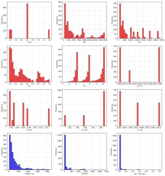
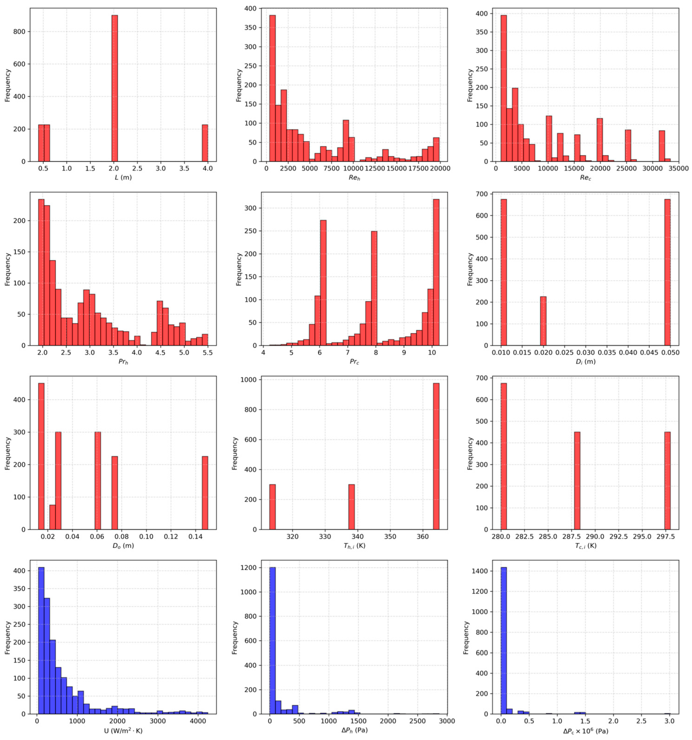
- Identification of the input features and output variables: The heat-transfer and fluid-flow physical phenomena in the concentric tube heat exchangers (CTHXs) are governed by several interacting physical parameters. Based on their relevance to the governing transport phenomena, nine key parameters were selected as input features for the ML models. These parameters include the length of the CTHX (), the inlet Reynolds number of the hot flow (), the inlet Reynolds number of the cold flow (), the Prandtl number of the hot fluid (), the Prandtl number of the cold fluid (), the inner-tube diameter (), the outer tube diameter (), and the inlet temperatures of the cold () and hot () fluids. The ML model aims to predict the thermo-hydraulic performance of CTHXs. In this context, the thermal performance is quantified using the overall heat-transfer coefficient (). In contrast, the hydraulic performance is assessed based on the pressure drops of the cold () and hot () flows. It is noteworthy that the input features were carefully selected based on an in-depth analysis of their physical relevance to the output variables, which characterize the governing physical phenomena of CTHXs. This procedure follows a feature selection strategy similar to that reported in [13]. Moreover, the distributions of all dataset variables, including the nine previously identified input features and the three output variables, are shown in Figure 2, as red and blue histograms, respectively.
- Feature standardization: The nine selected features were standardized using the StandardScaler available in the scikit-learn Python 3.7 library. This normalization of the input features ensures that all features contribute equally during ML model training by preventing variables with larger numerical ranges from dominating the learning process. On the other side, the output variables of the ML models, namely the overall heat-transfer coefficient (), the cold flow pressure drop () and the hot flow pressure drop (), were not scaled to maintain the physical interpretability.
- Data splitting: The dataset comprises 1575 samples. The train_test_split function from the scikit-learn Python library was used to divide the dataset into a training set (80%, 1260 samples) and a testing set (20%, 315 samples). The training set was exclusively used for training the ML models, whereas the test set was retained as unseen data for model evaluation and comparative analysis.
Figure 2.
Distributions of the nine input features (red histograms) and the three output variables (blue histograms) in the CFD-generated dataset.
4. Machine Learning Methodology
This section presents the detailed methodologies of the ANN and the PGNN.
4.1. Artificial Neural Network (ANN)
ANNs are among the most advanced machine learning (ML) techniques and are widely used across various fields due to their strong ability to capture complex patterns in data. The training process of ANNs generally involves two main stages: forward propagation and backward propagation. Initially, the weights and biases of each neuron in the network are randomly initialized. Subsequently, the input information propagates forward through the hidden layers to the output layer, where the network generates its prediction. The forward propagation process in each neuron of the ANN can be described as follows:
where is the bias vector, is the weight matrix and is the activation function. In the backward propagation process, the loss function is computed using the predicted output from the forward propagation and the actual (CFD) value. Then it is propagated backward from the output layer through the hidden layers until reaching the neurons of the input layer. The forward and backward propagation stages are iteratively repeated until the loss function converges to a minimum. The ANN’s loss function used in the present study is defined as follows:
where represent the CFD-derived (true) values of the output variables, denote the corresponding predicted values, is the index of the three output variables (, and ), is the number of samples in the mini-batch and is the L2 regularization coefficient. The ANN model was constructed using Keras with the Tensorflow Python library [35].
4.2. Physics-Guided Neural Network (PGNN)
The physics-guided neural network (PGNN) is an enhanced version of ANN that aims to incorporate the underlying physical phenomena of CTHXs into the learning process of the neural network through the loss function [36]. Empirical correlations are incorporated to constrain and guide the learning process, thereby improving the network’s ability to capture the heat-transfer and fluid-flow behavior within CTHXs and to predict their thermo-hydraulic performance (, and ) with high accuracy. More specifically, the physical guidance introduced in the present model operates at the level of the global thermo-hydraulic output quantities. For the thermal prediction, the Baehr–Stephan and Dittus–Boelter correlations relate the Nusselt number to the Reynolds number, Prandtl number, hydraulic diameter, and exchanger length, as presented in Equations (17) and (18). The resulting convective heat-transfer coefficients are subsequently combined through the overall thermal-resistance relation in Equation (20) to provide a correlation-based estimate of the overall heat-transfer coefficient. For the hydraulic predictions, the Darcy–Weisbach relation in Equation (21), together with regime-dependent friction-factor expressions, introduces the expected dependence of pressure drop on the length-to-diameter ratio, fluid density, velocity, and Reynolds number. The neural network does not replace these baseline relations; instead, it predicts non-negative multiplicative correction factors that account for deviations between the simplified correlations and the CFD-generated data.
These relations constitute the exact physical knowledge used to guide the present PGNN. However, the model does not explicitly evaluate the residuals of the continuity, momentum, or energy equations, nor does it enforce the local boundary and interface conditions used in the CFD simulations. Consequently, the model cannot guarantee local conservation of mass, momentum, or energy. The proposed framework should therefore be interpreted as a correlation-guided PGNN, rather than as a governing-equation-residual-based PINN or a fully physics-constrained neural network.
Therefore, the loss function of the PGNN relates the actual (CFD) values of the output variables with the values obtained from physical correlations by a non-negative correction factor . The loss function of the PGNN can be written as follows:
where are the values of the output variables (, and ) obtained using physical correlations. It should be noted that the PGNN does not directly predict the thermo-hydraulic performance parameters (, and ). Instead, the network predicts a non-negative correction factor (), which is applied to the empirical correlations to obtain the corrected predictions of the output variables. For computing the correlated overall heat-transfer coefficient (), Baehr and Stephan’s correlation [37] is first employed to calculate the Nusselt number () for the laminar flow regime, which can be expressed as follows:
where is the Graetz number expressed as , is the hydraulic diameter and is the length of the CTHX. For the turbulent-flow regime, the correlation developed by Dittus and Boelter [31] is used, and can be expressed as follows:
where n is 0.3 for the hot fluid (cooling process) and 0.4 for the cold fluid (heating process). After evaluating the Nusselt number in both the laminar and turbulent-flow regimes using the aforementioned correlations, the convective heat-transfer coefficients of the cold and hot fluids ( and ) can be directly calculated as follows:
where is the thermal conductivity of the cold or hot fluid (W·m−1·K−1). Subsequently, the correlated overall heat-transfer coefficient (Ũ) can be determined directly, assuming no wall and fouling resistances, as expressed in the following equation:
Regarding the hydraulic performance of CTHXs, the correlated pressure drops for the cold and hot fluids ( and ) are evaluated using the Darcy–Weisbach equation [38]:
where is the density of the cold or hot fluid, denotes the inlet velocity of the cold or hot fluid and is the friction coefficient of the cold or hot fluid. In the laminar flow regime, the friction coefficient is computed as [38], whereas in the turbulent-flow regime, it is calculated using [38]. Although the Reynolds number for the annular flow is evaluated using the hydraulic diameter, the classical friction-factor and Nusselt number correlations are employed only as baseline physical constraints within the PGNN model. To account for deviations associated with annular geometry, diameter ratio, and thermal boundary conditions, non-negative correction factors are incorporated into the PGNN loss function as presented in Equation (16). These correction factors enable the model to compensate for discrepancies between the classical correlations and the actual annular flow behavior while preserving the underlying physical trends.
4.3. Architecture and Input Parameters of the Neural Networks
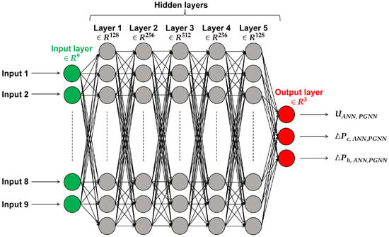
Starting with the neural network architecture, both the ANN and the PGNN share the same architecture. The network consists of an input layer with 9 neurons (corresponding to the number of input features), followed by 5 hidden layers containing 128, 256, 512, 256 and 128 neurons, respectively. The output layer comprises 3 neurons associated with the three output variables (, and ). The architecture of the ANN and PGNN models is illustrated in the schematic shown in Figure 3. For both the ANN and PGNN models, the Rectified Linear Unit (ReLU) function is employed as the activation function for the neurons in the hidden layers, and can be expressed as follows [39]:
Figure 3.
Architecture of the ANN and PGNN.
The ReLU function is commonly adopted for neural networks due to its ability to mitigate the vanishing gradient problems that may be encountered during the training process. As for the output layer, a linear function is used for the ANN, while a softplus activation function is employed for PGNN to ensure a non-negative correction factor , as defined by the following equation:
Gradient optimization is performed in both the ANN and PGNN models using the Adam optimizer [40] with an initial learning rate of 0.001. The reason for choosing the Adam optimizer is its ability to adapt the learning rate, leading to an accelerated optimization process. The Adam optimizer adjusts the weights and biases of the network’s neurons to reduce the loss function. L2 regularization is used to avoid overfitting with a regularization coefficient of 0.001. Moreover, a seed value of 42 is used for both the ANN and PGNN to ensure reproducibility and avoid randomness. Furthermore, the early stopping method was employed with a patience of 200 epochs, meaning that if the loss function did not improve in 200 epochs the training process will be stopped and the best weights that lead to the lowest Loss function will be restored. Lastly, the maximum number of epochs was set to 5000; however, due to early stopping, the training process typically converged in fewer epochs. The input parameters of the ANN and PGNN models are summarized in Table 5.
Table 5.
Summary of input parameters and training settings for ANN and PGNN models.
5. Results and Discussions
In this section, the mean absolute percentage error (MAPE) is used as a performance metric to evaluate the predictive accuracy of the ANN and PGNN models. It provides a clear and straightforward measure of the average percentage deviation between the CFD reference values and the model predictions, and can be computed as follows:
where is the number of samples in the training or test dataset.
5.1. Effect of Training Set Size
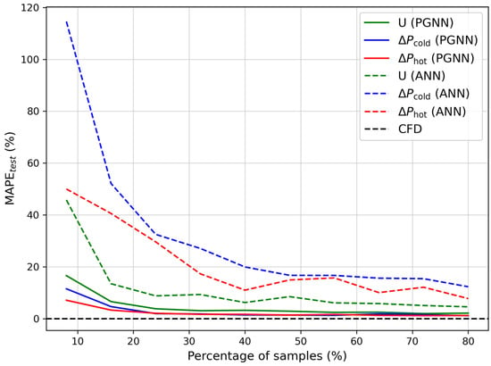
Figure 4 illustrates the variation in the MAPE, evaluated on the unseen test set, as a function of the sample percentage, defined as the ratio of training samples to the total number of samples. It is important to mention that the maximum sample percentage is limited to 80%, in accordance with the data-splitting strategy described in Section 3, where 80% of the dataset is allocated for training and the remaining 20% is reserved for testing and model performance comparison. Across a wide range of training set sizes, corresponding to percentages of samples between 8% and 80%, the test MAPE values of the three output variables , and obtained with the PGNN model (solid lines) are considerably lower than those of the ANN model (dashed lines). This demonstrates the superior predictive performance of the PGNN model compared to the ANN model in accurately capturing the complex physical phenomena of CTHXs, with minimal deviation from the CFD results (black dashed line). This improvement can be attributed to the integration of physics-based correlations into the learning process, which constrains the model and enhances its generalization capability.
Figure 4.
Variation in the MAPE evaluated on the unseen testing dataset function of the percentage of samples for the ANN and PGNN models.
Furthermore, even with a small training dataset of 315 samples (20% of the full set), the PGNN model exhibits negligible variation in MAPE compared to results obtained with the full training set (80%, i.e., 1260 samples). In contrast, for the ANN model, using 315 training samples results in a significant increase in MAPE compared to performance with the full training dataset. This reflects the robustness and high-fidelity of the PGNN model in predicting the thermo-hydraulic performance of CTHXs even when trained on small or moderate datasets. This also provides additional evidence of the PGNN model’s low sensitivity to training set size, especially within the range of 20% to 80% of the total samples.
5.2. Predictive Performance Comparison of the Neural Networks
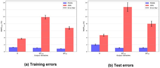
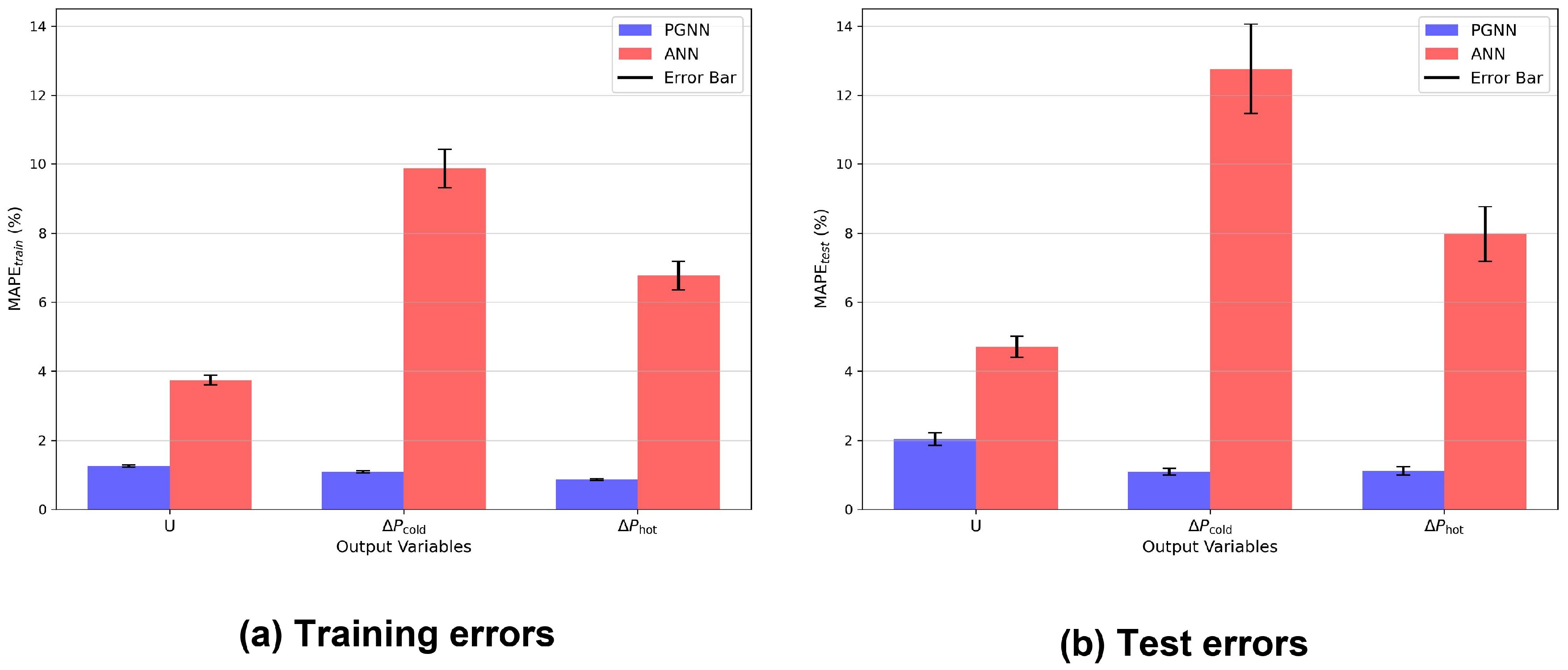
To provide a clear comparison of the predictive performance of the ANN and PGNN models on the training and unseen test datasets, histograms in Figure 5 show the MAPEs of the output variables evaluated on the training and test datasets using the full training set (1260 samples) and the test set (315 samples). The error bars shown in Figure 5 represent the standard deviation of the prediction errors, indicating the dispersion of the model predictions around the mean error values. For the PGNN model (blue bars), the MAPEs evaluated on the training set of the , and are 1.25%, 1.09% and 0.86%, respectively, whereas the MAPE calculated on the unseen test set are 2.03%, 1.09% and 1.11%, respectively. On the other side, the MAPEs for the ANN model (red bars) computed on the training data of the , and are 3.74%, 9.86% and 6.77%, while the corresponding test MAPEs are 4.71%, 12.75% and 7.97%, respectively. The prediction errors of the PGNN model on both training and test data are much smaller compared to those of the ANN model, particularly for predicting the hydraulic performance ( and ). This improved accuracy can be attributed to the incorporation of physical constraints into the PGNN’s loss function, which guides the neural network to account for the underlying physical phenomena of CTHXs during training. Furthermore, the results demonstrate the superior predictive performance of the PGNN model over the ANN model in assessing the thermo-hydraulic performance of CTHXs, with consistently small errors. In addition, the relatively small gaps between the training and test errors of the PGNN model indicate strong generalization performance and a reduced possibility of overfitting, as well as lower susceptibility to high-variance or high-bias scenarios.
Figure 5.
MAPEs of the output variables (, and ) for the PGNN and ANN models.
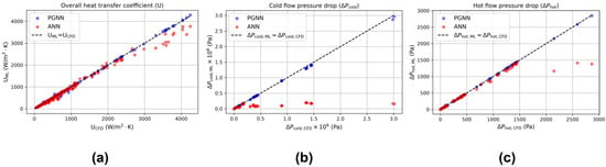
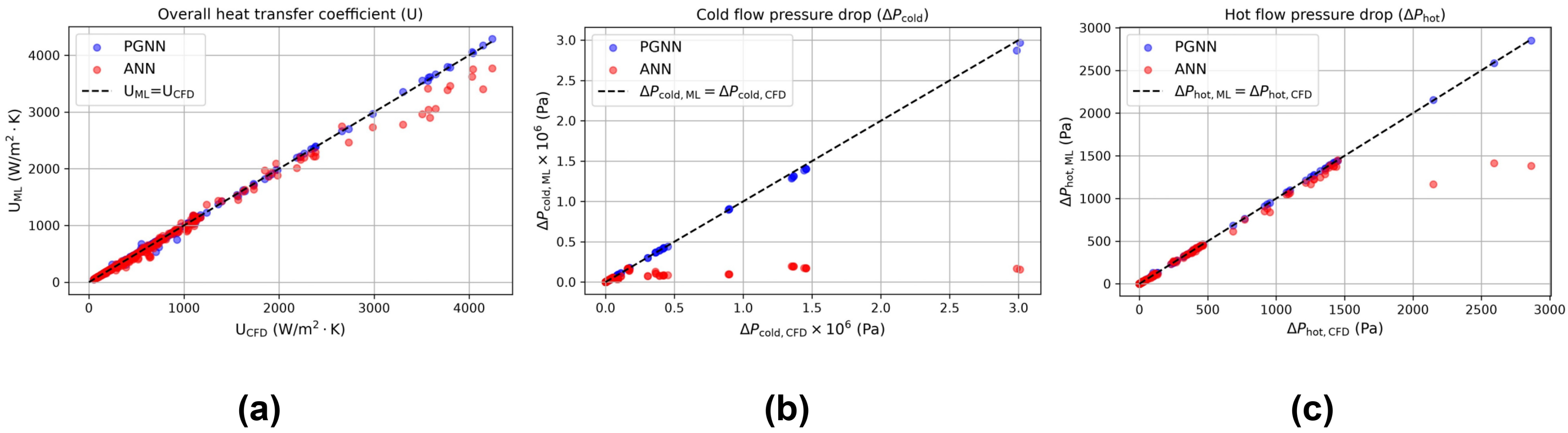
Figure 6a–c illustrate the variation in the , and predicted by the ANN and PGNN models over the unseen test dataset (315 samples) as a function of the corresponding values acquired using CFD simulations. For the PGNN model, the majority of the data points (blue) are closely clustered near the ideal black dashed line () for the three output variables , and with small deviations, elucidating the high fidelity of the PGNN model in accurately predicting the thermo-hydraulic performance of CTHXs. This tight clustering of the blue sample points near the perfect line demonstrates that the PGNN model neither underestimates nor overestimates the output variables, providing stable predictions across both training and test data. In contrast, the red data points of the ANN model deviate from the ideal theoretical line, particularly at higher values of the , and , reflecting the lower capability of the ANN model to generalize across the dataset and to deliver consistent predictions under a wide range of operating conditions of the CTHXs. At higher values of the output variables, the majority of ANN red points fall below the ideal line, indicating that ANN underestimates the values of the output variables in these regions. Furthermore, these results also serve as additional evidence to confirm the superior predictive accuracy of the PGNN model over the ANN model in estimating the thermal and hydraulic performances of CTHXs.
Figure 6.
Variation of (a) , (b) and (c) values predicted by the ANN (red points) and PGNN (blue points) models with respect to the corresponding values obtained using CFD simulations over the unseen test dataset.
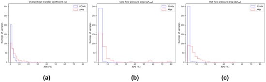
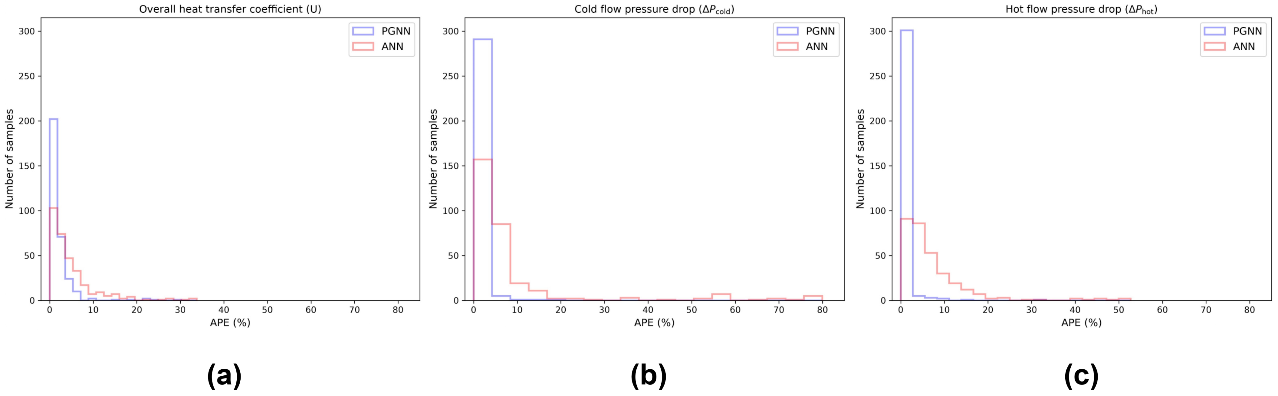
Additionally, Figure 7a–c show the absolute percentage error (APE) distribution of the , and , respectively, evaluated on the unseen test dataset. The majority of samples exhibit low APE values as indicated by the tallest histogram bar being concentrated in the low-APE regions. Notably, the PGNN model has a substantially higher number of samples with low APE values than the ANN model. For instance, for APE < 3%, the number of samples for is 265 for PGNN and 161 for ANN (Figure 7a), for it is 293 for PGNN versus 117 for ANN (Figure 7b), and for it is 305 for PGNN versus 98 for ANN (Figure 7c). Moreover, the ANN model shows outliers with APE values exceeding 35% for , whereas the PGNN model exhibits none across all output variables. This further highlights the PGNN model’s enhanced predictive accuracy over the ANN model, demonstrating its ability to precisely capture the physical phenomena of CTHXs by effectively mapping the complex relationships between input features and output variables.
Figure 7.
Absolute percentage error (APE) distribution of the (a) , (b) and (c) over the unseen test dataset.
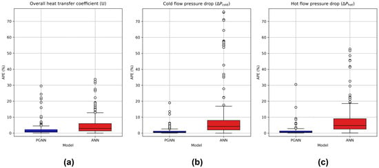
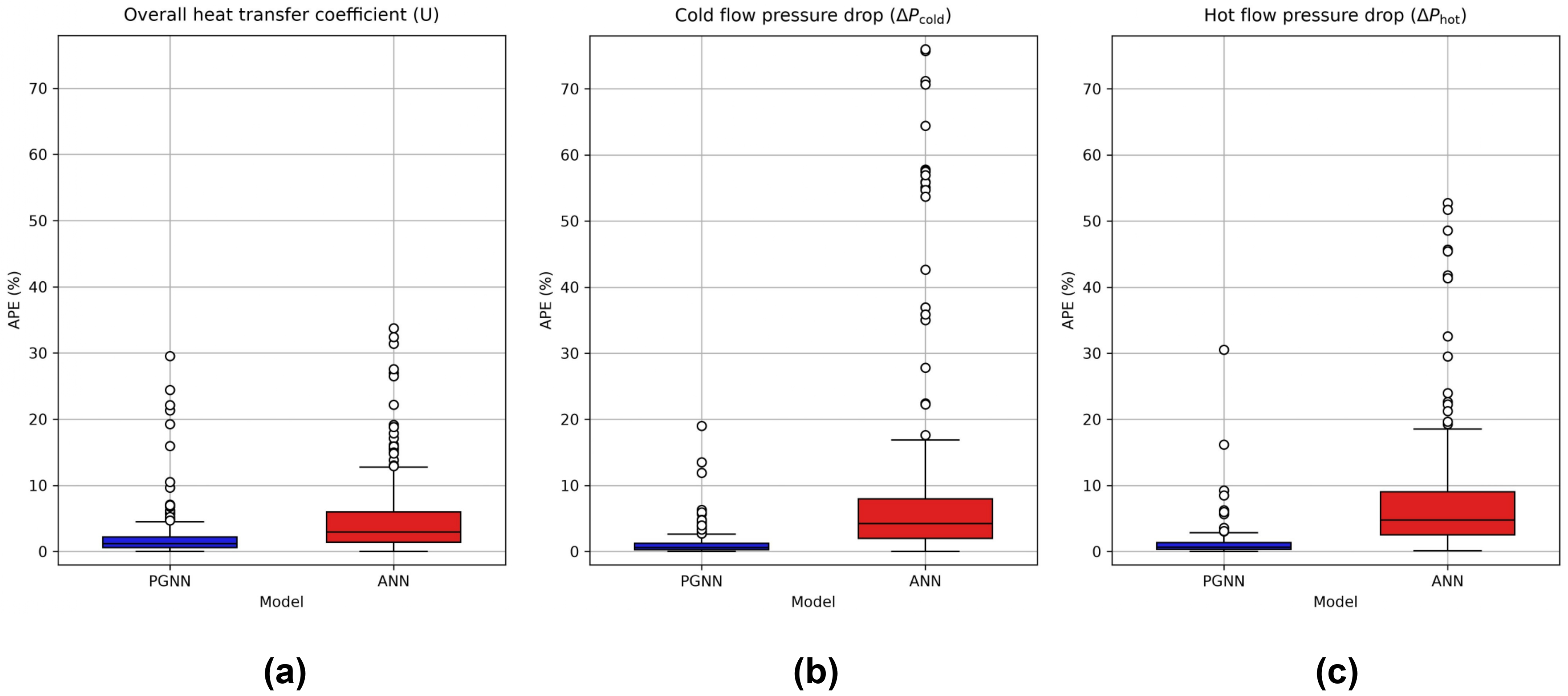
For further comparison of the predictive performance of the ANN and PGNN models, box plots of the APE are presented in Figure 8a–c for , and , respectively. It is noteworthy to mention that the box plots encompass the APE values for the unseen test dataset (315 samples). The APE box plots provide a comprehensive view of the error distribution across the entire dataset, emphasizing the key statistical percentiles: the first quartile (Q1, 25th percentile), the median (50th percentile), and the third quartile (Q3, 75th percentile). In each figure, the blue and red boxes correspond to the interquartile ranges of the PGNN and ANN models, respectively, bounded by Q1 and Q3, with the median indicated by a horizontal black line within each box. The whiskers extend beyond the interquartile range to represent the spread of APE values outside the central 50% of the data, reflecting moderate deviations. Data points lying beyond the upper whisker are identified as outliers. The APE values for the Q1, median and Q3 of the box plots for both ANN and PGNN models are summarized in Table 6. As shown in Figure 8, the APE boxes for the PGNN are all smaller and narrower than those of the ANN model for the three output variables , and , indicating lower APE values for Q1, median, and Q3, as presented in Table 6 compared to the ANN model. Moreover, across all box plots, the lower and upper whiskers of the PGNN model are noticeably shorter than those of the ANN model, indicating lower variability in APE values. This reflects a more consistent error distribution and consequently greater stability in the PGNN model’s predictions compared to the ANN model. Regarding outliers, the PGNN model exhibits no instances with APE values exceeding 35%. In contrast, the ANN model presents several outliers above this threshold, mainly in the predictions of and .
Figure 8.
Box plots of the (a) , (b) and (c) for the PGNN (blue) and ANN (red) models for the unseen test dataset.
Table 6.
Summary of the box plots.
6. Conclusions and Perspectives
In the present work, a physics-guided neural network (PGNN) approach is proposed to predict the thermo-hydraulic performance of CTHXs by estimating , and . The objective is to guide the neural network in capturing the underlying physical phenomena of the CTHXs by incorporating empirical correlations as constraints into the PGNN loss function. For comparison purposes, a standard artificial neural network (ANN) model was introduced with the same architecture and input parameters as the PGNN model. First, the effect of the training dataset size was investigated, revealing the PGNN model’s low sensitivity to it. In particular, between 20% (315 training samples) and 80% (1260 training samples) of the total dataset, the PGNN model exhibited only negligible changes in the MAPE evaluated on the unseen test set. In contrast, when using 20% of the dataset (315 samples) for training, the ANN model showed a significant increase in test MAPE values for the output variables, indicating a stronger dependence on the size of the training data. Moreover, the investigation of the training set size reveals that the PGNN model outperforms the ANN model, yielding lower MAPE values on the training and testing datasets for all output variables (, and ) across a wide range of training set sizes. Subsequently, a detailed error analysis was provided to compare the predictive performance of the ANN and PGNN models using the full training dataset (1260 samples, 80% of the total dataset). The results indicate that the MAPEs evaluated on the unseen test data for the , and using the PGNN model are 2.03%, 1.09% and 1.11%, respectively, which are remarkably lower than those obtained with the ANN model, which are 4.71%, 12.75%, and 7.97%, respectively. This demonstrates the superior predictive accuracy of the PGNN model compared to the ANN model in predicting the thermo-hydraulic performance of CTHXs. This enhanced predictive performance can be attributed to the inclusion of physical constraints in the loss function of the PGNN model, which enforce the neural network to consider the physical phenomena of the CTHXs during the training process.
Future work could extend the present approach by applying the proposed PGNN model to predict the thermo-hydraulic performance of other types of heat exchangers, such as plate heat exchangers. Another potential direction is to validate the CFD-based results by training the neural network on experimental data, thereby further assessing the model’s predictive capability under real-world conditions.
A limitation of the present study is the absence of direct experimental validation or a benchmark dataset reproducing the same concentric-tube geometry, boundary conditions, Reynolds number range, and thermal conditions. The empirical-correlation comparison and mesh-independence assessment provide numerical verification and consistency evidence, but they should not be interpreted as full validation. Experimental measurements of heat-transfer rates, outlet temperatures, and pressure drops will therefore be required to further establish the quantitative accuracy of the CFD-generated dataset and the resulting machine learning models.
A further methodological limitation concerns the level at which physics is incorporated into the proposed PGNN. The present framework uses empirical thermo-hydraulic correlations as global output-level guidance but does not include residuals of the continuity, momentum, or energy equations. Therefore, although the correlation-derived baselines introduce established heat-transfer and pressure-drop dependencies, the resulting predictions are not guaranteed to satisfy local conservation laws, boundary conditions, or conjugate-interface conditions. Moreover, because the current network maps global geometric and operating parameters directly to the global quantities , , and , it does not predict the spatial velocity, pressure, and temperature fields required to evaluate differential governing-equation residuals. The reported results should consequently be interpreted as those of a correlation-guided surrogate model rather than a fully equation-constrained model.
Another limitation is that the greywater stream is modeled as clean water and no fouling effects are considered. Actual greywater may contain suspended particles, detergents, fats, and other contaminants that can modify its effective viscosity and promote deposition on the tube walls. Such deposits may increase surface roughness and pressure losses, reduce the available flow area, and introduce an additional thermal resistance, thereby decreasing the overall heat-transfer coefficient and heat-recovery rate. The present results should therefore be interpreted as baseline predictions under clean-surface conditions. Future work should incorporate experimentally characterized greywater properties and time-dependent fouling resistance.
Another perspective is to investigate the influence of alternative Nusselt number, friction-factor, and pressure-drop correlations under different flow regimes and quantify how uncertainties in these correlations propagate through the correlation-guided loss function. More importantly, a governing-equation-residual-based extension of the present framework should be developed. Such an extension would require a field-based neural network architecture in which the spatial coordinates and operating conditions are provided as inputs and the local velocity, pressure, and temperature fields are predicted as outputs. The training loss could then combine CFD-data and correlation-guidance terms with residuals of the continuity, momentum, and energy equations, together with the inlet, outlet, wall, symmetry, and conjugate-interface boundary conditions. The simplified axisymmetric CTHX geometry considered in the present study provides a computationally tractable benchmark for developing and evaluating this extension. As an intermediate approach, integral energy conservation could also be introduced by jointly predicting the outlet temperatures and heat-recovery rate and penalizing any imbalance between the energy lost by the hot stream and that gained by the cold stream. These developments would permit a systematic comparison between purely data-driven, correlation-guided, integral-conservation-guided, and governing-equation-residual-based neural network formulations.
Author Contributions
Conceptualization, A.F., N.Y., S.A., J.F., A.A.S., K.C., A.M.A. and M.K.; Data curation, A.F. and S.A.; Formal analysis, A.F., N.Y., S.A., J.F., A.A.S., K.C., A.M.A. and M.K.; Investigation, A.F.,N.Y., S.A., J.F., A.A.S., K.C., A.M.A. and M.K.; Methodology, A.F., S.A. and M.K.; Validation, A.F. and S.A.; Writing—original draft, A.F.; Writing—review & editing, S.A., N.Y., J.F., A.A.S., K.C., A.M.A. and M.K.; Project administration, M.K. All authors have read and agreed to the published version of the manuscript.
Funding
This research received no external funding.
Data Availability Statement
The data presented in this study are available upon request from the corresponding author due to privacy and ethical restrictions.
Conflicts of Interest
The authors declare no conflict of interest.
Nomenclature
| Latin letters | |
| Coefficient of determination | |
| Length of CTHX (m) | |
| Reynolds number of the hot fluid | |
| Reynolds number of the cold fluid | |
| Prandtl number of the hot fluid | |
| Prandtl number of the cold fluid | |
| Inner-tube diameter of CTHX (m) | |
| Outer tube diameter of CTHX (m) | |
| Inlet temperature of the cold fluid (K) | |
| Inlet temperature of the hot fluid (K) | |
| Overall heat-transfer coefficient (W·m−2·K−1) | |
| Regularization coefficient | |
| Correlated output variables values | |
| Weight matrix | |
| Predicted output variables values | |
| Output variables obtained using CFD simulations | |
| Nusselt number | |
| Graetz number | |
| Hydraulic diameter (m) | |
| Friction coefficient | |
| Activation function | |
| Non-negative correction factor | |
| Convective heat-transfer coefficient of the cold fluid | |
| Convective heat-transfer coefficient of the hot fluid | |
| Density (kg·m−3) | |
| Inlet velocity (m·s−1) | |
| Number of samples | |
| Heat-recovery rate (W) | |
| Refining factor | |
| Turbulent kinetic energy | |
| Greek symbols | |
| Cold flow pressure drop (Pa) | |
| Hot flow pressure drop (Pa) | |
| Eddy viscosity | |
| Effectiveness | |
| Specific rate of dissipation | |
| Rate of dissipation | |
| Abbreviations | |
| PGNN | Physics-guided neural network |
| HX | Heat exchanger |
| HVAC | Heating ventilation and air conditioning |
| CTHXs | Concentric tube heat exchangers |
| CFD | Computational fluid dynamics |
| ML | Machine learning |
| ANN | Artificial neural network |
| ReLU | Rectified linear unit |
| MAPE | Mean absolute percentage error |
| PEC | Performance evaluation criteria |
| COP | Coefficient of performance |
| RANS | Reynolds-averaged Navier–Stokes |
| NTU | Number of transfer units |
References
- Kereikulova, A.; Yerdesh, Y.; Belyayev, Y.; Toleukhanov, A.; Botella, O.; Kheiri, A.; Khalij, M. Impact of Inlet Configuration and Flow Rates on Thermal Storage Stratification and Efficiency. Thermo 2026, 6, 16. [Google Scholar] [CrossRef] [Scilit]
- Garbai, L.; Santa, R.; Bošnjaković, M. Analysis of Thermodynamic Processes in Thermal Energy Storage Vessels. Thermo 2026, 6, 5. [Google Scholar] [CrossRef] [Scilit]
- Cavalerie, A.; Raymond, J.; Gosselin, L.; Rouleau, J.; Hakkaki-Fard, A. Sustainable Heating Analysis and Energy Model Development of a Community Building in Kuujjuaq, Nunavik. Thermo 2025, 5, 14. [Google Scholar] [CrossRef] [Scilit]
- Ignatkin, I.; Shevkun, N.; Skorokhodov, D. Investigation of the Influence of Wetting Ability of the Sprayed Surface of the Heat Exchanger on the Process of Evaporative Cooling. Thermo 2026, 6, 20. [Google Scholar] [CrossRef] [Scilit]
- Alsayah, A.M.; Alshukri, M.J.; Ali, S.; Faraj, J.; Khaled, M. Prediction of overall heat transfer coefficient in concentric tube heat exchangers using artificial neural networks: A comparative study with empirical correlations. Int. Commun. Heat Mass Transf. 2025, 163, 108723. [Google Scholar] [CrossRef] [Scilit]
- Ali, S.; Dbouk, T.; Khaled, M.; Faraj, J.; Drikakis, D. Morphing optimization of flow and heat transfer in concentric tube heat exchangers. Phys. Fluids 2023, 35, 095127. [Google Scholar] [CrossRef] [Scilit]
- Ali, S.; Habchi, C.; Zaytoun, H.; Khaled, M.; Dbouk, T. Surrogate-based optimization of the attack and inclination angles of a delta winglet pair vortex generator in turbulent channel flow. Int. J. Thermofluids 2023, 20, 100473. [Google Scholar] [CrossRef] [Scilit]
- Fawaz, A.; Hua, Y.; Le Corre, S.; Fan, Y.; Luo, L. Topology optimization of heat exchangers: A review. Energy 2022, 252, 124053. [Google Scholar] [CrossRef] [Scilit]
- Fawaz, A.; Hua, Y.; Le Corre, S.; Fan, Y.; Luo, L.; Biotteau, G. Topology optimization for dual-flow heat exchangers of moderate conductive material within a narrow design domain: Numerical and experimental investigations. Appl. Therm. Eng. 2025, 269, 125958. [Google Scholar] [CrossRef] [Scilit]
- Fawaz, A.; Hua, Y.; Le Corre, S.; Fan, Y.; Luo, L. Convergent-divergent design of fins for improving the thermo-hydraulic performance of heat exchangers assisted by a dual-flow topology generator. Therm. Sci. Eng. Prog. 2025, 65, 103948. [Google Scholar] [CrossRef] [Scilit]
- Fawaz, A.; Abed, A.F.; Alshukri, M.J.; Alsayah, A.M.; Ali, S.; Faraj, J.; Fahs, M.; Khaled, M. Random Forest Regressor-Driven Prediction of Solar Still Performance: A Fast and Accurate Alternative to CFD Simulations. Results Eng. 2025, 28, 107273. [Google Scholar] [CrossRef] [Scilit]
- Fawaz, A.; Hua, Y.; Le Corre, S.; Fan, Y.; Luo, L. A comparative study of objective functions in topology optimization for dual-flow heat exchanger of moderate conductive material: Toward improved thermo-hydraulic performance. Appl. Therm. Eng. 2026, 292, 130346. [Google Scholar] [CrossRef] [Scilit]
- Ali, S.; Faraj, J.; Awad, S.; Ramadan, H.S.; Khaled, M.; Dbouk, T. Innovative algorithmic approach of determining the overall heat transfer coefficient of concentric tube heat exchangers. Int. Commun. Heat Mass Transf. 2023, 148, 107077. [Google Scholar] [CrossRef] [Scilit]
- Sun, L.; Gao, H.; Pan, S.; Wang, J.-X. Surrogate modeling for fluid flows based on physics-constrained deep learning without simulation data. Comput. Methods Appl. Mech. Eng. 2020, 361, 112732. [Google Scholar] [CrossRef] [Scilit]
- Kapadia, H.; Feng, L.; Benner, P. Active-learning-driven surrogate modeling for efficient simulation of parametric nonlinear systems. Comput. Methods Appl. Mech. Eng. 2024, 419, 116657. [Google Scholar] [CrossRef] [Scilit]
- Hou, G.; An, Z.; Zhang, D.; Du, X.; Ding, Y.; Fu, J. Multi-variable operational data fusion and multi-scale hybrid modeling for online fouling monitoring of heat exchangers. Int. Commun. Heat Mass Transf. 2026, 175, 111129. [Google Scholar] [CrossRef] [Scilit]
- Colak, A.B.; Akgul, D.; Mercan, H.; Dalkılıç, A.S.; Wongwises, S. Estimation of heat transfer parameters of shell and helically coiled tube heat exchangers by machine learning. Case Stud. Therm. Eng. 2023, 42, 102713. [Google Scholar] [CrossRef] [Scilit]
- Haffejee, R.A.; Laubscher, R. Application of machine learning to develop a real-time air-cooled condenser monitoring platform using thermofluid simulation data. Energy AI 2021, 3, 100048. [Google Scholar] [CrossRef] [Scilit]
- Willard, J.; Jia, X.; Xu, S.; Steinbach, M.; Kumar, V. Integrating Scientific Knowledge with Machine Learning for Engineering and Environmental Systems. ACM Comput. Surv. 2023, 55, 1–37. [Google Scholar] [CrossRef] [Scilit]
- Abdulkarim, A.H.; Nooruldeen, O.; Ghareeb, A.; Akgül, D.; Mercan, H.; Dalkilic, A.S. Physics-Guided Machine Learning and Deep Neural Networks for Accurate and Robust Heat Transfer Predictions in Shell and Helical Coil Heat Exchangers. Arab. J. Sci. Eng. 2025, 51, 9253–9280. [Google Scholar] [CrossRef]
- Bokil, G.R.; Geyer, T.F.; Merbold, S.; Kazula, S. Physics-Guided Convolutional Neural Network for Flow Prediction in Heat Exchangers in Electrified Aircraft. In AIAA Aviation Forum and Ascend 2024; American Institute of Aeronautics and Astronautics: Las Vegas, NV, USA, 2024. [Google Scholar] [CrossRef] [Scilit]
- Raissi, M.; Perdikaris, P.; Karniadakis, G.E. Physics-informed neural networks: A deep learning framework for solving forward and inverse problems involving nonlinear partial differential equations. J. Comput. Phys. 2019, 378, 686–707. [Google Scholar] [CrossRef] [Scilit]
- Liang, X.-Y.; Zhang, B.; Zhang, C.-L. Physics-informed deep residual neural network for finned-tube evaporator performance prediction. Energy 2024, 302, 131822. [Google Scholar] [CrossRef] [Scilit]
- Cai, S.; Wang, Z.; Wang, S.; Perdikaris, P.; Karniadakis, G.E. Physics-Informed Neural Networks for Heat Transfer Problems. J. Heat Transf. 2021, 143, 060801. [Google Scholar] [CrossRef] [Scilit]
- Majumdar, R.; Jadhav, V.; Deodhar, A.; Karande, S.; Vig, L.; Runkana, V. HxPINN: A hypernetwork-based physics-informed neural network for real-time monitoring of an industrial heat exchanger. Numer. Heat Transf. Part B Fundam. 2025, 86, 1910–1931. [Google Scholar] [CrossRef] [Scilit]
- Shan, L.; Wu, Q.; Wang, M.; Zhang, H.; Li, W.; Guo, Y.; Shao, S.; Chen, Z.; Liang, Y. A novel physics-guided collaborative modeling method for steady-state simulation of air source heat pump system. Int. J. Refrig. 2026, 181, 317–331. [Google Scholar] [CrossRef] [Scilit]
- Bergman, T.L.; Lavine, A.S.; Incropera, F.P.; DeWitt, D.P. Introduction to Heat Transfer; John Wiley & Sons: Hoboken, NJ, USA, 2011. [Google Scholar]
- Menter, F.R. Two-equation eddy-viscosity turbulence models for engineering applications. AIAA J. 1994, 32, 1598–1605. [Google Scholar] [CrossRef] [Scilit] [PubMed]
- ANSYS, Inc. ANSYS Fluent, Release 2023 R1 [Computer Software]; ANSYS, Inc.: Canonsburg, PA, USA, 2023; Available online: https://www.ansys.com (accessed on 1 May 2025).
- Celik, I.B.; Ghia, U.; Roache, P.J.; Freitas, C.J. Procedure for estimation and reporting of uncertainty due to discretization in CFD applications. J. Fluids Eng.-Trans. ASME 2008, 130, 078001. [Google Scholar] [CrossRef] [Scilit]
- Dittus, F.W. Heat transfer in automobile radiators of the tubular type. Univ. Calif. Pub. Eng. 1930, 2, 443–461. [Google Scholar] [CrossRef] [Scilit]
- Pethukov, B.S.; Kirillov, V.V. The problem of heat exchange in the turbulent flow of liquids in tubes. Teploenergetika 1958, 4, 63–68. [Google Scholar]
- Gnielinski, V. New equations for heat and mass transfer in turbulent pipe and channel flow. Int. Chem. Eng. 1976, 16, 359–367. [Google Scholar]
- Cengel, Y.A.; Ghajar, A.J. Heat and Mass Transfer (in SI Units); Mcgraw-Hill Education-Europe: London, UK, 2014; ISBN 10:0071311122. [Google Scholar]
- Abadi, M.; Agarwal, A.; Barham, P.; Brevdo, E.; Chen, Z.; Citro, C.; Corrado, G.S.; Davis, A.; Dean, J.; Devin, M.; et al. TensorFlow: Large-Scale Machine Learning on Heterogeneous Distributed Systems. arXiv 2016, arXiv:1603.04467. [Google Scholar]
- Robinson, H.; Pawar, S.; Rasheed, A.; San, O. Physics guided neural networks for modelling of non-linear dynamics. Neural Netw. 2022, 154, 333–345. [Google Scholar] [CrossRef] [Scilit] [PubMed]
- Kreith, F.; Bohn, M.; Kirkpatrick, A. Principles of Heat Transfer. J. Sol. Energy Eng. 1997, 119, 187. [Google Scholar] [CrossRef] [Scilit]
- Brown, G.O. The History of the Darcy-Weisbach Equation for Pipe Flow Resistance. In Environmental and Water Resources History; American Society of Civil Engineers: Washington, DC, USA, 2002; pp. 34–43. [Google Scholar] [CrossRef] [Scilit]
- Agarap, A.F. Deep Learning using Rectified Linear Units (ReLU). arXiv 2018, arXiv:1803.08375. [Google Scholar]
- Kingma, D.P.; Ba, J. Adam: A Method for Stochastic Optimization. arXiv 2014, arXiv:1412.6980. [Google Scholar]

Disclaimer/Publisher’s Note: The statements, opinions and data contained in all publications are solely those of the individual author(s) and contributor(s) and not of MDPI and/or the editor(s). MDPI and/or the editor(s) disclaim responsibility for any injury to people or property resulting from any ideas, methods, instructions or products referred to in the content. |
© 2026 by the authors. Licensee MDPI, Basel, Switzerland. This article is an open access article distributed under the terms and conditions of the Creative Commons Attribution (CC BY) license.