


Abstract
Converting waste carbon dioxide (CO2) into value-added chemicals is a central strategy for the circular carbon economy and for decoupling industrial activity from fossil carbon, directly supporting Sustainable Development Goal (SDG) 7 (Affordable and Clean Energy), SDG 9 (Industry, Innovation and Infrastructure), SDG 12 (Responsible Consumption and Production), and SDG 13 (Climate Action). The photocatalytic conversion of CO2 to formic acid (HCOOH) represents a promising dual-purpose route within this strategy: it simultaneously valorises atmospheric or industrial CO2 and enables safe, liquid-phase chemical hydrogen storage for the renewable energy transition. The RK-X technology, employing a homogeneous, biocompatible, silver-containing fulvic acid-based catalyst under visible light irradiation at ambient temperature and moderate CO2 pressure, has previously demonstrated the production of formic acid from CO2 and water. Building on this established reaction, 22 preliminary photocatalytic experiments were performed across a range of process conditions, with formic acid concentration determined by permanganometric (redox) titration (strictly, permanganate-oxidisable species expressed as formic acid equivalents). These measurements were used to identify physically grounded factor–response models, based on Henry’s Law, saturation kinetics, a power-law irradiance dependence, and Michaelis–Menten-type catalyst saturation, describing how pressure, reaction time, light output, and catalyst concentration govern formic acid yield. A Python-based computational framework (version: Python 3.9.6) then used these calibrated models to construct complete, balanced full factorial Design of Experiments (DoE) matrices, enabling the structure of the factorial design space to be explored beyond the scope of the original measurement set with the aim of limiting further physical experimentation, reagent consumption, and energy expenditure (a saving that is not quantified in this work). It is emphasised throughout that these matrices are model-generated rather than measured: the framework is an experiment-planning and screening tool, not a substitute for experimental measurement, and the analysis presented here does not constitute empirical validation of the RK-X reaction mechanism. A 24 DoE was first constructed with the four process factors, pressure [bar], reaction time [h], light output [kW], and catalyst concentration [mg/L], each at two levels, augmented with five center points. After statistical evaluation in TIBCO® STATISTICA (version 13.3), all main effects and two-factor interactions were found significant, and a significant curvature effect indicated the need for a three-level design. A subsequent 34 DoE was analysed, in which a quadratic-by-linear reaction time × catalyst concentration term reached significance in the analysed realisation but proved weak and scale-dependent in a sensitivity analysis across noise levels and random seeds, and is therefore not interpreted as a process finding. The transferability of the workflow was then assessed by re-parameterising the same framework for a related RK-X reaction producing ethanol; this is an assessment of methodological portability, not an independent experimental validation, although the physically executed pilot-scale ethanol measurements underlying this assessment are validated by a companion, independently peer-reviewed study. Because the analysed responses are generated by the calibrated models themselves, the reported p-values, curvature tests and pure-error estimates quantify the resolving power of the design under an assumed variance structure rather than providing independent evidence about the physical system; every conclusion is conditional on the calibrated models. A direct factorial analysis of the measured preliminary runs, which form a 24 design with five genuine replicates, shows strong curvature and, on a logarithmic scale, a single pressure × reaction time interaction that the separable model lacks; a revised model, propagation of parameter uncertainty, a simulated comparison of alternative designs and a two-stage follow-up plan are reported, and all code and datasets are provided. Interpreted on this basis, the work offers a transferable methodology, intended to be resource-efficient, for prioritising and sequencing the physical experiments required to develop and scale emerging CO2 utilization and renewable hydrogen storage technologies.
Keywords:
carbon dioxide utilization; circular carbon economy; green chemistry; photocatalytic formic acid synthesis; design of experiments; model-based experimental design; renewable hydrogen storage; resource-efficient process optimization; simulation-based experimental planning; computer experiments; Sustainable Development Goals; STATISTICA 1. Introduction
1.1. The Global Challenge of CO2 Accumulation
The accelerating accumulation of carbon dioxide (CO2) in Earth’s atmosphere constitutes one of the foremost environmental challenges of the twenty-first century. Driven primarily by the combustion of fossil fuels, large-scale deforestation, and industrial processes, atmospheric CO2 concentrations have reached levels unprecedented in human civilization. According to the World Meteorological Organization, the global average CO2 concentration reached approximately 423.9 ppm in 2024, a value roughly 50% above pre-industrial levels, and the annual growth rate between 2023 and 2024 was 3.5 ppm, the largest single-year increase since systematic measurements commenced in 1957 [1]. The International Energy Agency has further reported that total energy-related CO2 emissions reached a record 37.8 Gt in 2024 [2]. As carbon sinks, including oceans and terrestrial ecosystems, progressively lose their absorptive capacity, the atmospheric residence of anthropogenic CO2 intensifies the greenhouse effect, driving global mean temperature rises that have surpassed 1.3 °C above pre-industrial baselines [3].
Conventional approaches to CO2 management have focused predominantly on carbon capture and geological storage (CCS), yet these strategies remain energy-intensive and economically prohibitive at the scale required. An alternative and increasingly compelling paradigm is the chemical utilization of CO2 as a feedstock, transforming what is currently regarded as the terminal product of the fossil fuel value chain into a renewable carbon source for the synthesis of value-added chemicals [4]. This approach embodies the principle of carbon circularity: rather than permanently sequestering CO2, it is incorporated into commodity chemicals that can substitute for fossil-derived precursors, thereby closing the carbon loop and reducing net atmospheric emissions.
The valorisation of waste streams as secondary raw materials is a broader and well-established strategy for lowering the carbon intensity of industrial activity, and it has been pursued across very different material systems: the incorporation of industrial solid wastes such as red mud into low-carbon binders, for example, simultaneously displaces a carbon-intensive primary material and diverts a hazardous residue from disposal [5]. Chemical CO2 utilization can be understood within the same logic, with the distinguishing feature that the waste stream is gaseous, dilute and thermodynamically stabilised, so that valorisation requires an external energy input, in the present case supplied as visible light.
This circular carbon economy paradigm aligns directly with several Sustainable Development Goals (SDGs). Converting a waste stream into a value-added chemical feedstock supports SDG 12 (Responsible Consumption and Production) and SDG 9 (Industry, Innovation and Infrastructure) by enabling more resource-efficient, lower-impact industrial processes; when the resulting product also serves as a hydrogen carrier, it further contributes to SDG 7 (Affordable and Clean Energy); and, by mitigating net CO2 emissions, the approach directly advances SDG 13 (Climate Action). Realizing this potential at scale, however, requires efficient process development methodologies capable of characterizing and optimizing novel CO2 utilization technologies without imposing prohibitive experimental, material, and energy costs of their own, a methodological need that motivates the present study.
1.2. Photocatalytic CO2 Conversion to Formic Acid
Among the products accessible from CO2 reduction, formic acid (HCOOH) has attracted scientific and industrial interest. As the simplest carboxylic acid, formic acid is a valuable platform chemical with applications in leather tanning, textile processing, food preservation, and as a reducing agent in organic synthesis [6]. Crucially, it also constitutes a viable liquid organic hydrogen carrier (LOHC), with a hydrogen content of 4.4 wt% and a volumetric hydrogen density of 53 g L−1 [7]. The photocatalytic reduction of CO2 to formate/formic acid is thermodynamically accessible via a two-electron transfer
representing the energetically most favourable multi-electron CO2 reduction product [8].
CO2 + 2H+ + 2e− → HCOOH (E° = −0.25 V vs. NHE at pH = 7),
Photocatalytic routes to formic acid have been explored using a variety of catalytic systems, including titanium dioxide (TiO2)-based semiconductors [9], palladium-decorated metal oxides [10] and metal–organic frameworks (MOFs) [11]. Pan and Heagy provided a comprehensive review of photocatalytic CO2 reduction to formate, emphasizing the critical roles of charge separation efficiency, CO2 adsorption capacity, and intermediate stability in determining product selectivity [8]. More recently, Köntös et al. reported the successful conversion of CO2 to formic acid employing an organic, homogeneous, fulvic acid-based catalyst (RRR catalyst) in an aqueous medium under light irradiation at room temperature, achieving concentrations of up to 8.47 g/L of formic acid [4]. This technology, referred to herein as the RK-X process, employs a homogeneous, silver-containing fulvic acid-based catalyst rather than a conventional heterogeneous metal-oxide photocatalyst, represents a genuinely green chemistry approach, and offers the additional advantage that the CO2 substrate is derived directly from dissolved gas, making the process directly compatible with point-source capture or atmospheric CO2 streams.
The overall reaction catalysed in the RK-X system may be schematically represented as:
CO2 + H2O → HCOOH + ½O2
The mechanism draws an analogy to natural photosynthesis, where light energy drives the endergonic fixation of CO2(aq) into organic molecules via the excited electronic states of the catalyst. The use of fulvic acid, a naturally occurring, low-molecular-weight humic substance, as the photosensitizer and catalytic scaffold is particularly noteworthy, as it is biocompatible, widely available, and inherently chromophoric across the UV-Vis spectrum [4].
1.3. Formic Acid as a Hydrogen Storage Vector
Hydrogen is increasingly recognized as a cornerstone of the post-fossil energy transition and a key enabler of SDG 7 (Affordable and Clean Energy): it can be produced from renewable electricity via electrolysis and, when consumed, yields only water as a by-product. However, the infrastructure challenges associated with hydrogen’s physical storage and transport remain a major barrier to its widespread deployment. Gaseous hydrogen has an extremely low volumetric energy density and, due to its minute molecular diameter, permeates most conventional containment materials, causing embrittlement and presenting safety hazards [12]. Cryogenic liquid storage at −253 °C and high-pressure compression at 350–700 bar are technically demanding and energetically costly [13].
Formic acid circumvents these limitations by functioning as a liquid-phase hydrogen carrier at ambient temperature and pressure. The reversible cycle is straightforward: CO2 hydrogenation to formic acid stores hydrogen covalently, and catalytic dehydrogenation then releases CO2-free hydrogen on demand [7,14]. Several studies have established homogeneous and heterogeneous catalytic systems for high-turnover formic acid dehydrogenation under mild conditions [15,16]. The implementation of formic acid as an LOHC within a CO2-based synthesis loop is thus synergistic: it has been proposed as a pathway to hydrogen storage that simultaneously valorises atmospheric or industrial CO2 streams [17]; whether it is net-beneficial depends on its life-cycle performance, which is not assessed in this work (Section 4).
1.4. Design of Experiments as a Tool for Process Optimization
Systematic optimization of multi-variable chemical processes requires efficient statistical methodologies. The one-variable-at-a-time (OVAT) approach, varying a single factor while fixing all others, is both inefficient and incapable of detecting interaction effects between process variables. Design of Experiments (DoE) provides a principled alternative: by constructing structured factorial matrices in which all factor combinations are examined simultaneously, DoE enables quantification of individual factor effects, pairwise and higher-order interactions, and curvature effects with a greatly reduced number of experimental runs [18].
Full factorial designs of the 2k type, where k factors are each investigated at two levels, are widely employed for factor screening and interaction identification in chemical process development [19]. Weissman and Anderson provided a comprehensive survey of DoE applications to active pharmaceutical ingredient (API) synthesis, illustrating how factorial analysis accelerates route scouting and scale-up [20]. The extension to three-level (3k) designs enables the fitting of quadratic response surface models, which are necessary when significant curvature effects are detected in the initial two-level screen [21]. Center points, added to two-level designs, serve a dual purpose: they provide additional degrees of freedom for error estimation and allow a formal curvature check prior to committing to the full three-level design [18].
A distinction that is central to the present work, and that is not always made explicitly in the applied DoE literature, must be drawn at this point. Classical Design of Experiments, in the tradition established by Fisher [22] and developed for industrial practice by Box and co-workers [23], is an inferential methodology: randomisation, replication and blocking are the devices by which an observed response difference is licensed to support a causal claim about the physical system, and the p-values produced by ANOVA acquire their meaning from the fact that the error term is estimated from genuinely independent physical replicates. Nothing in that logic survives the substitution of simulated responses for measured ones.
Model-based or predictive experimental design occupies a different epistemic position. Here a calibrated mechanistic or semi-empirical model is used to generate responses across a design space, and the resulting analysis characterises the model and the design rather than the physical system directly. This is the domain of the design and analysis of computer experiments [24], of Bayesian calibration and model-discrepancy analysis [25], and of model-based design of experiments for parameter precision [26], where the accepted role of the simulation is to identify which physical experiments are worth performing and where in the factor space they should be located. Numerical models of this kind are routinely used to explore operating spaces that would be prohibitive to map exhaustively by measurement, in fields ranging from process engineering to the prediction of transport phenomena in complex geometries [27]. The framework presented in this paper belongs unambiguously to this second category. Its outputs are hypotheses about factor importance and design adequacy, to be tested against measurement; they are not themselves measurements, and they are not presented as such.
The application of DoE to emerging photocatalytic CO2 conversion processes is, to our knowledge, largely unexplored in the primary literature. The principal barrier is the paucity of experimental data sufficient to characterize factor–response relationships prior to planning the factorial matrix. In the present work, we address this gap by developing a Python-based computational framework that constructs complete factorial datasets from empirical models calibrated against a preliminary campaign of real photocatalytic measurements. This allows candidate factorial designs to be evaluated on a balanced experimental space before any of their grid points is measured; it informs, but does not replace, the measurements themselves.
1.5. Aims and Scope of This Work
This study reports:
- The development of a Python-based DoE data framework for the RK-X photocatalytic CO2-to-formic acid process;
- The execution and statistical analysis of 24 and 34 factorial designs in TIBCO® STATISTICA, including significance tests for main effects, interaction effects, and curvature;
- The re-parameterisation of the framework for a related RK-X process yielding ethanol, for which only the reaction-time response has been measured;
- An explicit statement of the epistemic scope of model-generated factorial designs, distinguishing what such an analysis can and cannot establish about the physical process;
- A direct factorial analysis of the measured preliminary runs, a revised model including the pressure × reaction time interaction found there, and noise-level, random-seed, parameter-uncertainty and design-comparison analyses that bound the model-based conclusions;
- A discussion of the implications for process intensification and scale-up.
The methodology represents a transferable blueprint for planning the DoE-based optimization of novel heterogeneous and homogeneous catalytic processes where real experimental data are scarce. It is explicitly not a substitute for such data: the intended output is a prioritised, defensible physical experimental programme, and the framework is of value precisely because it allows that programme to be designed before scarce reagent, reactor time and analytical capacity are committed. This distinction is most consequential when the eventual objective is industrial-scale deployment of CO2 utilization technology: the physical experimental burden of mapping a multi-factor design space exhaustively grows sharply with scale, so that a defensible, model-informed basis for prioritising which conditions to measure first, rather than attempting exhaustive physical coverage, becomes progressively more valuable as the target throughput moves from laboratory to pilot to industrial scale. By evaluating candidate factorial designs on models calibrated against a comparatively small preliminary measurement campaign, the approach also embodies core sustainability principles of resource efficiency and waste minimization in early-stage green chemistry development, with the aim of reducing the reagents, energy, and time that would otherwise be required to physically execute a full multi-level factorial campaign; this reduction is not quantified in the present work.
2. Materials and Methods
2.1. The RK-X Photocatalytic Process
The RK-X technology converts CO2 dissolved in water into formic acid in the presence of a homogeneous, fulvic acid-based catalyst under light irradiation. A proof-of-concept experiment demonstrated the feasibility of the reaction using 1 L of CO2-saturated water containing the catalyst exposed to natural sunlight for two weeks [4]. Two additional controlled laboratory experiments served as reference datasets for parameterizing the computational model [4,28].
2.2. Preliminary Experimental Campaign
To characterize the RK-X process across its relevant operating range, 22 preliminary photocatalytic experiments were performed, varying pressure, reaction time, light output, and catalyst concentration individually and in combination around the reference conditions. The individual run conditions and the measured responses (permanganate-oxidisable species expressed as formic acid equivalents) are reported in full in Table 1, and the reference conditions themselves are summarized (see Section 3.1). The response of each sample was determined by permanganometric (redox) titration; the procedure, reagents, standardisation, uncertainty components and selectivity limitations of the method are described in Section 2.2.1. Runs 1–16 of Table 1 form a complete 24 full factorial design (5 and 8 bar; 1 and 4 h; 10 and 30 W; 100 and 300 mg/L), runs 17–21 are five replicated centre points (6.5 bar, 2.5 h, 20 W, 200 mg/L), and run 22 (7.0 bar, 3.0 h, 25 W, 250 mg/L) is one additional run. This preliminary dataset served as the empirical basis for estimating the parameters of the factor–response relationships described in Section 2.3, which were subsequently used to construct the full factorial design matrices analysed in this study; the measured factorial itself is analysed directly in Section Direct Factorial Analysis of the Measured Runs and Revised Model Form.
Table 1.
Conditions and measured responses (permanganate-oxidisable species expressed as formic acid equivalents, mg/L) of the 22 preliminary RK-X photocatalytic experiments that form the empirical basis of the factor–response models in Section 2.3. The measurement uncertainty of the titration method is characterised in Section 2.2.1. Recorded T is a single manual reading taken at the end of each run, not a continuous instrumented record (see Section 2.2.2).
All experiments were performed in a jacketed, magnetically stirred, gas-tight photoreactor charged with 1.7 L of deionised water, pressurised with CO2 to the stated set point and irradiated by the visible-light source at the stated electrical output. Irradiance up to 30 W, pressures up to 8 bar and reaction times up to 4 h cannot be assumed to leave the bulk temperature unperturbed; the temperature record for the preliminary campaign, and the resulting constraint on the interpretation of the factor–response models, are reported in Section 2.2.2.
2.2.1. Determination of Formic Acid by Titration: Procedure, Standardisation and Selectivity
Aliquots of the reactor liquor were withdrawn at the end of each run, filtered, purged of residual dissolved CO2, and titrated against standardised potassium permanganate solution. The titrant was standardised against oxalic acid. Each sample was titrated in triplicate, and the reported concentration is the mean of the three determinations. The combined standard uncertainty was estimated from the standard deviation of the replicate titrations, the uncertainty of the titrant concentration, the burette and volumetric glassware tolerances, and the end-point detection uncertainty; the resulting expanded uncertainty (k = 2, approximately 95% coverage) was not calculated on a per-run basis, and a full method-level uncertainty budget combining all these components has not yet been computed. A partial, empirical estimate of the method’s run-to-run precision is nonetheless available from the design of the preliminary campaign itself: five of the 22 runs (Table 1, runs 17–21) were independent physical replicates at a single fixed condition, giving a directly measured relative standard deviation of 2.7% (mean = 50.0 mg/L, SD = 1.34 mg/L, n = 5; 95% confidence interval for the true relative standard deviation, from the chi-squared distribution on 4 degrees of freedom, approximately 1.6–7.7%). This estimate is used in Section 2.4 to assess, rather than merely assume, the noise magnitude applied in the model-generated factorial designs.
The selectivity limitation of this method is stated plainly here. Permanganometric titration is a redox method: it quantifies the permanganate-oxidisable content of the sample and does not measure acidity. It does not identify formic acid, and it cannot distinguish formic acid from any other permanganate-oxidisable species that may be present, including the fulvic acid-based catalyst itself and its degradation products, oxalic acid, glycolic acid, or other partially oxidised C1–C2 products. The measured values in Table 1 are therefore correctly described as permanganate-oxidisable species expressed as formic acid equivalents, and they cannot be interpreted as the formic acid concentration alone. The method was adopted for the preliminary campaign because it is rapid, inexpensive and adequate for establishing the relative ordering of factor effects, which was the purpose of that campaign. It is not adequate to establish product identity, selectivity, or a carbon balance, and no such claim is made in this work. Matrix-matched blanks, recovery tests and chromatographic measurements across the conditions of Table 1 are not part of the data reported here; within the data reported here, chromatographic verification is limited to the reference concentration presented in Section 3.1. (accredited external HPLC, ref. [28]) and the t = 2 h point of Run 1 for ethanol (see Section 3.4); further HPLC confirmation for the ethanol system is reported in the companion study reported in Section 3.4. Throughout this manuscript, the response variable is to be understood in this restricted sense.
2.2.2. Temperature Control and Monitoring
Bulk liquid temperature was not continuously instrumented; no calibrated in-situ probe or data logger was used during the 22 preliminary runs; the reactor was operated at ambient laboratory temperature without active thermostatting or temperature monitoring. This is a genuine limitation of the preliminary campaign rather than an implicit claim of isothermality: because temperature governs CO2 solubility through the Henry coefficient and enters the apparent kinetic constants of every step in the mechanism, any systematic drift in bulk temperature correlated with irradiance or pressure would be confounded with the corresponding factor effect, and this possibility cannot be excluded retrospectively. The factor–response models of Section 2.3 should accordingly be read as conditional on the unmeasured, presumed-ambient temperature range of the preliminary campaign. Temperature is not treated as a factor in the designs analysed here; it is a candidate fifth factor, and direct temperature logging is part of the follow-up campaign described in Section 4, while its inclusion as an explicit factor is left to a later stage. The “Recorded T” values reported alongside each run in Table 1 are a single manual temperature reading taken at the end of each run rather than a continuous, calibrated bulk-liquid record; they are reported for completeness and as a qualitative check, but do not constitute the instrumented temperature monitoring that would be needed to rule out the confounding described above, which remains an open limitation.
2.3. Empirical Factor–Response Models
Semi-empirical models relating each process factor to the formic acid response were identified from the preliminary experimental campaign (Section 2.2), based on physicochemical reasoning and the measured reference data. The four factors investigated were pressure (p, bar), reaction time (t, h), light output (I, kW), and catalyst concentration (cat, mg/L). The dependent variable was formic acid concentration [HCOOH] (mg/L).
The pressure factor operates indirectly: increased system pressure enhances CO2 solubility in water according to Henry’s Law, thereby increasing the effective substrate concentration available for the photocatalytic reaction. For pressure, a direct linear proportionality was assumed, reflecting the linear dependence of dissolved CO2 concentration on pressure at constant temperature in the Henry’s Law regime [29]:
yp = p
For reaction time, a saturation-type kinetic model was adopted rather than a simple linear function, because the finite amount of dissolved CO2 substrate imposes an upper limit on product accumulation at extended reaction times [30]. The model takes the form of a first-order approach to equilibrium
where τ is the characteristic time constant, set to the literature-typical value of 2 h (the fitted value is given below). For light output, a power-law relationship was used, reflecting the sub-linear dependence of quantum yield on irradiance observed in many photocatalytic systems [30]
with α = 0.5 (literature-typical). For catalyst concentration, a Michaelis–Menten-type saturation model was selected, analogous to enzyme kinetics, to capture the observed saturation behaviour at high catalyst loadings [31]
where Kc is the half-saturation constant, set to the literature-typical value of 100 mg/L.
yt = 1 − e−t/τ
yI = Iα
ycat = cat/(Kc + cat)
The literature-typical values of the three adjustable constants of Equations (2)–(4), namely the characteristic time constant τ, the irradiance exponent α and the half-saturation constant Kc, were checked against the preliminary campaign by a joint nonlinear least-squares regression against all 22 runs (Table 1); because the campaign is a 24 factorial with centre points rather than a set of one-factor-at-a-time sweeps, the parameters were fitted jointly. The functional forms themselves were selected a priori on physicochemical grounds—linear Henry’s Law behaviour for pressure, first-order approach to equilibrium for time, sub-linear power-law dependence of quantum yield on irradiance, and Michaelis–Menten-type saturation for catalyst loading—and were not selected by comparison of fit quality across competing forms, because the preliminary dataset is too small to support such model discrimination. This is a genuine limitation: the data are consistent with the assumed forms but do not uniquely identify them, and alternative saturating functions would fit comparably well. The fitted parameter values and their standard errors, together with the overall fit statistics (number of runs, coefficient of determination and residual standard deviation) of the joint regression, are reported in Table 2.
Table 2.
Estimated parameters of the semi-empirical factor–response models (Equations (1)–(4)), obtained by nonlinear least-squares regression against the preliminary experimental campaign, with associated fit statistics. n, R2 and the residual standard deviation describe the single joint regression from which all four rows were obtained simultaneously and are therefore identical across rows; they are not four independent single-parameter fits. These fitted values are reported here as a diagnostic of model adequacy; they were not adopted as the operating parameter set of Table 3a (see text).
Table 3.
(a) Model-generated 24 factorial design matrix with factor levels and model-predicted HCOOH responses. All response values in this table are computed from Equations (1)–(5) with the literature-typical parameter set of Section 2.3 and include an independent draw of the multiplicative noise term (normally distributed, relative standard deviation 5%) for each of the 16 corner points and 5 centre points. (b) Comparison factorial design matrix, computed with the fitted parameter set from the joint regression of Section 2.3 and Table 2 (τ = 2.60 h, α = 0.468, Kc = 92.9 mg/L) in place of the literature-typical set used for Table 3a (τ = 2 h, α = 0.5, Kc = 100 mg/L). Factor levels are identical to Table 3a; only the predicted HCOOH concentration differs; the values in this table are noise-free model predictions. This table has not been imported into STATISTICA and is not the basis of the ANOVA, Pareto charts or Figure 1, Figure 2, Figure 3, Figure 4 and Figure 5.
Figure 1.
Results of the statistical analysis for the 24 formic acid DoE (model-generated data of Table 3a: pressure 5–8 bar, reaction time 1–4 h, light output 3.3–10 kW, catalyst concentration 100–300 mg/L; 16 corner points and 5 centre points; 5% multiplicative noise): (a) ANOVA table of all effects and interactions. (b) ANOVA table after pooling insignificant effects into the error term, evaluating statistically significant effects. (c) Pareto chart of standardized effects found to be statistically significant.
Figure 2.
Residual plots for the 24 formic acid DoE (model-generated data of Table 3a), used to check whether the data follow a normal distribution: (a) Plot of predicted values and raw residuals; no systematic trend in the mean of the residuals is observed, while their spread is expected to increase with the predicted value under multiplicative noise (Section 2.5). (b) Dot plot of predicted and observed values; the points align with the reference line, indicating agreement between observed values and the assumed model. (c) Normal probability plot of residuals; the points align with the reference line, indicating that the residuals follow the expected normal distribution.
Figure 3.
Results of the statistical analysis for the 34 formic acid DoE (model-generated 81-run matrix: factor ranges as in Table 3a with an intermediate level for each factor; 5% multiplicative noise): (a) ANOVA table of all effects and interactions. (b) ANOVA table after pooling insignificant effects into the error term, evaluating statistically significant effects. (c) Pareto chart of standardized effects found to be statistically significant.
Figure 4.
Interaction plots of reaction time [h] and catalyst concentration [mg/L] for the 34 formic acid DoE (model-generated data): (a) Means plot of the two factors, showing that the model-predicted response increases with both factors. (b) Surface plot of the two factors, showing the nonlinear relationship between them.
Figure 5.
Residual plots for the 34 formic acid DoE (model-generated data), used to check whether the data follow a normal distribution: (a) Plot of predicted values and raw residuals; no systematic trend in the mean of the residuals is observed, while their spread is expected to increase with the predicted value under multiplicative noise (Section 2.5). (b) Dot plot of predicted and observed values; the points align with the reference line, indicating agreement between the observed values and the assumed model. (c) Normal probability plot of residuals; the points align with the reference line, indicating that the residuals follow the expected normal distribution. (d) Histogram of raw residuals; the bars follow the superimposed normal curve, indicating a normal distribution.
In this regression the right-hand sides of Equations (1)–(4) were multiplied together with an overall scale constant k (the pressure term of Equation (1) has no free parameter), using the Levenberg–Marquardt algorithm as implemented in SciPy. Here k is a lab-scale proportionality constant specific to the 1.7 L preliminary campaign (k = 3.60 ± 2.07 mg/L, in the units of Equations (1)–(4)); it is distinct from, and not to be confused with, the industrial-scale reference value HCOOHref = 768 mg/L of Table 4, which enters only the normalized construction of Equation (5) used to build Table 3a. The fit converged to τ = 2.60 ± 1.26 h, α = 0.468 ± 0.150, and Kc = 92.9 ± 59.3 mg/L (n = 22, R2 = 0.809, adjusted R2 = 0.777, residual standard deviation = 11.1 mg/L); these values, together with the corresponding fit statistics, are reported in Table 2. The residuals are not random with respect to the factor levels: the model over-predicts every run at 5 bar (by up to 23 mg/L at 4 h) and the runs at 8 bar and 1 h, fits the runs at 8 bar and 4 h closely, and under-predicts the five centre-point replicates (by 8–12 mg/L) and run 22 (by 16 mg/L) (Table S1b). This pattern indicates a pressure–time interaction, or a departure from strict multiplicativity, that the assumed separable model does not capture, and it is the reason the fit is reported here as a diagnostic rather than adopted as a validated calibration. A lack-of-fit test against the pure error of the five replicates confirms this formally (F(14,4) = 88.1, p < 0.001; Table S1). Because of this identified lack of fit, and for continuity with the independent reference point of Table 4, Section 3.1, Section 3.2, Section 3.3 and Section 3.4 and the model-generated design of Table 3a continue to use the literature-typical parameter set (τ = 2 h, α = 0.5, Kc = 100 mg/L) rather than the newly fitted values above; the two parameter sets are close but not identical, the model form is revised in Section Direct Factorial Analysis of the Measured Runs and Revised Model Form, and the design analyses are repeated with the fitted and the revised parameter sets in Section 3.6. Table 3b, in Section 3.1, gives the factorial design matrix recomputed with the fitted parameter set for direct, point-by-point comparison against Table 3a. The investigated factor ranges for pressure, reaction time and catalyst concentration (5–8 bar, 1–4 h, 100–300 mg/L) were set by the operating envelope of the preliminary campaign, and the corresponding design levels lie inside, or at the boundary of, the range spanned by the calibration data (Table 1). The light-output range of the designs (3.3–10 kW) was instead set by the 3.3 kW lighting blocks of the larger-scale reactor (Section 3.4) and does not lie within the range of the calibration data, which spans 10–30 W in the 1.7 L preliminary campaign: the lowest design level exceeds the highest calibration level by a factor of 110. The relative span between the low and high light-output levels is comparable (a factor of about 3 in both cases), but in absolute terms the light-output dependence of the model-generated responses is an extrapolation from the calibration data, anchored for the formic acid system only by the single measured reference point of Table 4 (6.6 kW) through Equation (5).
Direct Factorial Analysis of the Measured Runs and Revised Model Form
Runs 1–21 of Table 1 were also analysed directly as a 24 full factorial with five centre points, with all main effects and interactions and a curvature contrast; the five genuine replicates supply a pure-error estimate with 4 degrees of freedom (Table S2). On the measured scale, all four main effects, all six two-factor interactions and the curvature contrast are significant (p < 0.02). Reaction time (effect 27.4 mg/L), pressure (22.3 mg/L), light output (13.7 mg/L) and catalyst concentration (9.3 mg/L) rank in that order, pressure × reaction time is the largest interaction (16.7 mg/L), and the centre-point mean (50.0 mg/L) exceeds the corner mean (25.9 mg/L) by 24.0 mg/L. Because a multiplicative response turns separate factor effects into apparent interactions on the measured scale (Section 2.5), the analysis was repeated on the logarithm of the response. On the logarithmic scale only the four main effects, the pressure × reaction time interaction (p < 0.001) and the curvature contrast remain significant; no other interaction reaches p = 0.05 (Table S2). The measured data are therefore consistent with a separable multiplicative structure except in two respects. First, pressure and reaction time interact: at 1 h, raising the pressure from 5 to 8 bar increases the response by a factor of 1.5–1.7, as expected from Henry’s Law, whereas at 4 h it increases it by a factor of 2.9–3.0. Second, the centre points lie well above any separable surface through the corners. Which factor or factors carry this curvature cannot be resolved from a two-level design with centre points; resolving it is the first objective of the follow-up campaign (Section 4).
To revise the model form, the separable model was extended by a single pressure–time interaction term on the logarithmic scale, y = k · y_p · y_t · y_I · y_cat · exp(γ · z_p · z_t), where z_p and z_t are pressure and reaction time coded to −1…+1 over 5–8 bar and 1–4 h. The joint fit gives τ = 2.03 ± 0.85 h, α = 0.467 ± 0.130, Kc = 93.2 ± 51.7 mg/L and γ = 0.164 ± 0.079 (R2 = 0.858, adjusted R2 = 0.825, residual standard deviation 9.9 mg/L; AICc 108.8 compared with 112.0 for the separable form; Table S1). The revision reduces but does not remove the lack of fit (F(13,4) = 70.4, p < 0.001), because the remaining misfit is concentrated at the centre points, which the separable saturating terms cannot raise sufficiently. The revised form is therefore used in Section 3.6 as a second working hypothesis, not as a validated calibration. The pressure and reaction-time ranges of the designs coincide with those of the calibration data, so the interaction term is not extrapolated; the light-output caveat stated above applies unchanged.
2.4. Model-Based Construction of the Factorial Design
A Python script was developed to construct a complete, balanced factorial experimental matrix from the calibrated factor–response models described in Section 2.3, following the general principle of model-based Design of Experiments (MBDoE) [26]. The overall model equation is constructed as a product of the reference HCOOH value and normalized factor effects:
y = HCOOHref × effp × efft × effI × effcat
Each factor effect is defined as the ratio of the factor’s model equation evaluated at the DoE factor level to the same equation evaluated at the reference experimental conditions. This normalization ensures that all factor effects take values near unity, keeping the model-predicted output about the reference observation and thereby maintaining physical plausibility. A normally distributed multiplicative noise term with a relative standard deviation of 5% was applied to each grid point (an independent draw for every run of every matrix, including each of the 16 corner points and 5 centre points of Table 3a). The draws were generated with NumPy as numpy.random.default_rng(42).normal(1, 0.05, n), applied in the run order of Table 3a and, for the 34 matrices, in lexicographic order of the coded levels with pressure varying slowest; this reproduces Table 3a and the STATISTICA output of Figure 1 and Figure 3 exactly (Supplementary Code S1, Table S3). This term is an assumed variance structure, not an observed one: it is a pseudorandom perturbation drawn from a distribution chosen by the analyst, and it does not reproduce the correlation structure of the true experimental variability of the RK-X system. The magnitude of the assumed 5% is, however, not an unconstrained choice. The preliminary campaign already contains five genuine physical replicates at a fixed condition (Table 1, runs 17–21: 6.5 bar, 2.5 h, 20 W, 200 mg/L). These five titrations give a directly measured relative standard deviation of 2.7% (mean = 50.0 mg/L, SD = 1.34 mg/L, n = 5). Because this estimate is itself based on only five replicates, its own sampling uncertainty is appreciable: a chi-squared interval on the variance (4 degrees of freedom) gives a 95% confidence interval for the true relative standard deviation of approximately 1.6% to 7.7%. The 5% value assumed throughout Section 3.2, Section 3.3 and Section 3.4 therefore lies within this empirically derived interval and is not an arbitrary order-of-magnitude guess; it is a defensible, if imprecise, estimate of the titration method’s replicate variability under the present protocol. The sensitivity of the significance decisions to noise levels bracketing this measured value (2%, 2.7%, 5% and 8%) and to the random seed is reported in Section 3.5. In addition to the 24 = 16 corner points, five centre points were computed by evaluating all factor models at their midpoint values and applying five independent draws of the noise term. These are not replicates in the experimental sense and they contain no information whatever about pure experimental error. They estimate only the dispersion of the imposed noise distribution. Consequently, the quantity that STATISTICA reports as pure error in the analyses below is, in this work, an estimate of the assumed simulation variance, and the curvature and lack-of-fit tests built upon it must be read as diagnostics of the design and the model rather than as tests against physical measurement error. The script exports the complete factorial matrix, including factor levels and model-predicted HCOOH responses, to an Excel (.xlsx) file; all matrices are provided in Data S1. The same framework was subsequently adapted for the ethanol-producing variant of the RK-X process. The reaction-time sub-model was re-parameterised using the fitted time constant reported in Section 3.4 (τ = 1.67 h, from the ethanol time-course data of Table 5); the pressure, light-output and catalyst-concentration sub-models retain the exponents and constants of the formic acid system (α = 0.5, Kc = 100 mg/L) by analogy, as these three factors were not independently varied in the ethanol experiments and are correspondingly unverified for this reaction. The normalization reference point for the ethanol design (EtOHref = 12 mg/L) is the accredited HPLC measurement itself, taken at the same conditions under which it was measured (8 bar, 2 h, 3.3 kW, 250 mg/L; Table 5), so that the ethanol design matrix is anchored to a real measurement in the same manner as the formic acid design is anchored to HCOOHref (Table 4).
2.5. Statistical Analysis
Statistical evaluation was performed in TIBCO® STATISTICA (version 13.3). The formic acid analyses were replicated in Python by ordinary least squares on the same coded model terms, reproducing the STATISTICA effect estimates, t-values and residual mean squares of Figure 1 and Figure 3; the ethanol analysis (Figure 6) and the additional analyses of Section Direct Factorial Analysis of the Measured Runs and Revised Model Form, Section 3.5 and Section 3.6 were performed in Python (Supplementary Code S1). The imported datasets were analysed using the dedicated Design of Experiments module. Significance of main effects, interactions, and curvature effects was assessed by analysis of variance (ANOVA) using an F-test, with effects deemed significant at p < 0.05. Non-significant effects were progressively pooled into the residual error term, and the impact of this pooling on the significance of remaining effects was monitored. Normal distribution of residuals was verified using the Shapiro–Wilk test and by visual inspection of normal probability plots of standardized residuals.
Figure 6.
Standardised effects (Pareto charts) for the 34 ethanol DoE (model-generated 81-run matrix; factor ranges as in Table 3a; ethanol model of Section 2.4 normalised to the reference measurement of Table 5, 12 mg/L at 8 bar, 2 h, 3.3 kW, 250 mg/L; 5% multiplicative noise, seed 42; analysed in Python): (a) all 32 terms (residual df = 48); (b) after pooling by the rule of Section 2.5. Blue bars, p < 0.05; grey bars, not significant; dashed line, p = 0.05. The 16 largest terms are shown; the full ANOVA tables are given in Table S8a,b.
The analysis proceeded in a fixed sequence. Effects were estimated by ordinary least squares on the coded factor levels. The full model for the two-level design comprised four main effects, six two-factor interactions, four three-factor interactions and the curvature contrast, with the four-factor interaction pooled with the pure error; for the three-level design it comprised linear and quadratic main effects and their linear-by-linear, linear-by-quadratic and quadratic-by-quadratic interactions. Significance was assessed by F-tests against the residual mean square at α = 0.05. Effects were then pooled into the residual term in ascending order of their absolute standardised effect, one at a time, with the significance of every surviving term re-examined after each pooling step; pooling was halted when the next candidate term reached p < 0.10, following the conservative recommendation that terms of marginal significance should not be absorbed into the error estimate. Both the unpooled and the pooled ANOVA tables are reported for every design, so that the effect of this decision is visible to the reader.
Model adequacy was assessed by the coefficient of determination and its adjusted form, by the residual standard deviation relative to the mean response, and by the lack-of-fit F-test where the design supported one. The ANOVA assumptions were checked as follows: normality of the standardised residuals by the Shapiro–Wilk test and by normal probability plots; homogeneity of variance by inspection of residuals against fitted values, noting that a multiplicative noise model necessarily produces variance that increases with the mean and that this is visible in the residual plots; and independence by the ordering of runs, which for a computationally generated matrix is trivially satisfied and correspondingly uninformative. Pareto charts of standardised effects are reported to convey the relative magnitude of effects, which is the quantity of practical interest for experimental planning, rather than significance alone. To separate genuine non-additivity from the scale effect of multiplicative noise, every design was additionally analysed on the logarithm of the response, on which multiplicative noise is homoscedastic and a separable multiplicative model has no interaction terms.
2.6. Scope and Epistemic Status of the Model-Generated Designs
Because this point conditions the interpretation of every result that follows, it is stated here in full rather than deferred to the Discussion.
The factorial matrices analysed in Section 3 are generated by evaluating Equations (1)–(5) at the design points and adding pseudorandom noise. The ANOVA performed on those matrices therefore decomposes variance that was, by construction, put there by the analyst. Three consequences follow and are accepted without qualification. First, the finding that all main effects and all two-factor interactions are significant is an algebraic consequence of the multiplicative model form of Equation (5), which makes every pairwise product term non-zero, combined with a low noise level relative to the factor effects; it is not a discovery about the RK-X reaction. Second, the detection of curvature is an algebraic consequence of the nonlinearity of Equations (2) and (4), which was imposed a priori. Third, the p-values, F-statistics and pure-error estimates reported below have no direct experimental interpretation: they are properties of the design, the model and the assumed noise distribution, and they cannot be used to support any inference about the physical mechanism, the identity or selectivity of the products, the carbon balance, or the true experimental uncertainty of the process.
What the analysis can legitimately establish is narrower but not trivial and is of practical use to a process development programme. It establishes that the calibrated factor–response model system, taken as a working hypothesis, implies a response surface whose curvature cannot be resolved by a two-level design, so that a two-level screening campaign executed on the real system would be inadequate and a three-level design is the correct next physical experiment. It establishes the relative magnitudes of the effects that such a campaign would need to resolve, and hence the number of runs and the analytical precision required to resolve them, subject to the parameter uncertainty quantified in Section 3.6, under which only the dominance of reaction time is robust. It identifies where the model is least certain and where the measured data already contradict it—above all the pressure × reaction time interaction and the curvature at the centre of the design (Section Direct Factorial Analysis of the Measured Runs and Revised Model Form)—and therefore where physical runs carry the highest information value. And, through the ethanol case in Section 3.4, it illustrates that the workflow can be re-parameterised for another reaction system within the RK-X family; only the reaction-time response of that system was tested against measurement. These are statements about experimental strategy, and they remain useful even though they are conditional on the model, because the alternative in early-stage development is to plan the campaign on no quantitative basis at all.
The correct reading of this manuscript is therefore as a contribution to experimental planning methodology, illustrated on a CO2 utilization system, and not as an experimental study of that system. The analysis does not confirm that the RK-X reaction behaves in accordance with physicochemical theory: such a claim would be circular, because the responses are generated by the models themselves. The sustainability argument is likewise set out in Section 4: any resource saving would arise from performing fewer, better-targeted physical experiments, not from replacing them. To state this without any remaining ambiguity: the physical validation campaign described in Section 4 is a precondition for any claim about the RK-X reaction itself—its product identity, selectivity, carbon balance, or yield under the conditions examined here—as distinct from a claim about the Design-of-Experiments planning methodology, which is the contribution this manuscript makes.
3. Results
Before presenting the statistical outputs below, readers are referred to Section 2.6, which states the epistemic status of every ANOVA, curvature and significance result that follows: these are properties of the calibrated model system and the assumed noise structure, not empirical findings about the RK-X reaction.
3.1. Model-Generated Factorial Dataset, Formic Acid (24 DoE)
The calibrated factor–response models described in Section 2.3 were used to construct a complete, model-generated 24 factorial matrix comprising 16 corner-point runs and 5 center-point replicates for the formic acid reaction (Table 3a).
Across the 16 corner points, the fitted-parameter predictions in Table 3b differ from the noise-free literature-typical predictions (Equations (1)–(5) before the noise term is applied, on which the responses in Table 3a are based) by between −5.9% and +11.1%, and the centre-point prediction differs by +2.3%. The deviations are systematic rather than random: at the short-reaction-time level (t = 1 h) the fitted set predicts lower HCOOH concentrations than the literature-typical set, while at the long-reaction-time level (t = 4 h) it predicts higher concentrations. This is the same pressure–time interaction identified from the residuals of the joint regression (Section 2.3): the separable multiplicative model cannot represent it with either parameter set, so neither table should be read as more than an interpolation aid pending the physical validation campaign of Section 4.
The STATISTICA software correctly identified the dataset structure of Table 3a as a 24 full factorial design with five center points. The reference experimental conditions used for normalization are summarized in Table 4 [28]. This reference point is drawn from prior published RK-X characterisation at a larger operating scale than the 22-run preliminary campaign of Table 1 [28]. Unlike the 22 preliminary runs of Table 1, which were quantified by on-site redox titration against potassium permanganate for practical reasons (the reactor is operated in a container remote from full laboratory infrastructure, so a rapid field method was required), the reference HCOOH concentration reported in [28] was verified by accredited external high-performance liquid chromatography (HPLC) analysis rather than by the field titration method. Because Equation (5) uses only the dimensionless ratio of each factor level to this reference, the construction is internally consistent, and the central anchor point of the normalization is therefore grounded in an accredited physical measurement rather than an assumed or purely modelled value. This does not, however, convert Table 3a,b into an experimentally validated dataset: the single reference value from [28] anchors the scale of the normalization, but it is not part of the calibration dataset used to fit Equations (1)–(4), and it does not constitute multi-point validation of the design grid itself, which remains model-generated. This scale gap, and the distinction between the accredited anchor point and the still-simulated design grid, are discussed further in Section 2.3 and Section 4.
Table 4.
Reference conditions taken from prior published RK-X characterisation [28], used for normalization of the factor effects in Equation (5). The reference HCOOH concentration (768 mg/L) was quantified there by accredited external HPLC analysis, distinct from the permanganometric field titration used for the 22-run preliminary campaign of Table 1 (Section 2.2.1). These reference conditions are drawn from a larger-scale system distinct from the 22-run preliminary campaign of Table 1; the resulting scale gap between the calibration data and this normalization reference is discussed in Section 2.3 and Section 4.
3.2. ANOVA Results, Two-Level Factorial (24)
Following import and analysis in STATISTICA, all four main effects (pressure, reaction time, light output, catalyst concentration) and all six two-factor interactions were found to be statistically significant at p < 0.05. As set out in Section 2.6, this outcome is a property of the multiplicative model form of Equation (5) rather than an empirical finding, and it is reported here because the magnitudes of the effects, not their significance, are what inform the design of the subsequent physical campaign. The curvature check was also significant (p < 0.05), indicating that the model response surface exhibits nonlinear behaviour in the investigated factor space (Figure 1). Across 1000 independent noise realisations at 5% (Section 3.5), the main effects and the curvature contrast are significant in every realisation, but the two-factor interactions are not equally robust: pressure × reaction time, reaction time × light output and reaction time × catalyst concentration are detected in at least 98% of realisations, pressure × light output in 90%, light output × catalyst concentration in 80% and pressure × catalyst concentration in 67%. On the logarithmic scale none of the two-factor interactions are significant, confirming that they arise from the multiplicative model form.
This finding justified the progression to a three-level factorial design. Residual analysis confirmed that the normality assumption was acceptable, as evidenced by the residual plots (Figure 2).
3.3. ANOVA Results, Three-Level Factorial (34)
The dataset was extended to the 34 = 81-run matrix by introducing an intermediate (center) level for each factor. Consistent with expectations, the linear main effects of all four factors and all linear-by-linear two-factor interactions were significant (Figure 3).
In the analysed realisation, the quadratic-by-linear interaction between the squared reaction time term (t2) and catalyst concentration (cat) was also significant (p = 0.028). This term should not be over-interpreted. Across 1000 noise realisations it is detected in only 28% at 5% noise (62% at the measured 2.7%; Section 3.5); it is not significant when the matrix is recomputed with the fitted (p = 0.056) or the revised parameter set (p = 0.22; Section 3.6); and on the logarithmic scale it vanishes, being detected in 7% of realisations, close to the nominal false-positive rate. It is thus a weak, scale-dependent consequence of multiplying two saturating functions. What is scale-independent is the shape of the constant-yield contours: within the calibrated model, an increase in catalyst concentration can partially substitute for an increase in reaction time, so that the two factors trade off along a curved locus of constant yield rather than a straight line.
Because both Equations (2) and (4) are saturating, the exchange rate between the two factors is not constant but varies across the design space, and any single multiplier quoted for it would be an artefact of the operating point at which it is evaluated, and no such multiplier is given; establishing the exchange rate quantitatively requires physical measurement along the relevant contour and is identified as a priority experiment in Section 4 (Figure 4).
Normality of residuals was confirmed (Figure 5).
3.4. Transferability Assessment: Application of the Framework to the RK-X Ethanol Variant
This section assesses transferability, not validation: whether the same computational workflow, re-parameterised, produces an internally coherent design and analysis for a second reaction system within the RK-X family, and whether the sequential design logic (two-level screen, curvature test, escalation to three levels) reaches a sensible conclusion there as well. A positive result demonstrates portability of the method; it says nothing about whether the ethanol reaction behaves as modelled.
The ethanol-producing variant of the RK-X process was operated in the same 1600 L continuous stirred tank reactor used for the formic acid reference measurement (Table 4) [28], with the RRR fulvic-acid catalyst replaced by a VMMM nickel-based catalyst at 250 mg/L, matching the loading convention of the formic acid reference condition [32]. The reactor was charged with 8 bar CO2 and illuminated at 3.3 kW, half the light output used for the formic acid reference (6.6 kW). Light output on both variants of the reactor is supplied by a modular LED array built from independently switchable 3.3 kW lighting blocks, so that only discrete multiples of 3.3 kW are physically available (one, two or three blocks: 3.3, 6.6 and 9.9 kW, reported throughout as 3.3, 6.6 and 10 kW); the same three block settings define the light-output levels of the formic acid design (Section 2.4, Table 3a) and are reused unchanged for the ethanol design below. For this first ethanol run, a single active block (3.3 kW, the lowest available setting) was used as a deliberate, conservative starting point; the formic acid reference condition instead uses two active blocks (6.6 kW). One consequence of this choice is that the ethanol reference point sits at the low end, rather than the centre, of the shared 3.3–10 kW design range, so the normalised light effect in the ethanol design only increases from unity (never decreases) across the investigated range—unlike the formic acid design, where the reference is roughly central. This is a direct consequence of which block was switched on for this first run, not an inconsistency in the modelling, and it is noted explicitly here for transparency. The reaction was quasi-isothermal (25–30 °C), as the lower light input released substantially less heat than the formic acid configuration and no active cooling was required. Ethanol concentration was determined by classical redox titrimetry, analogous in principle to the permanganometric determination of formic acid (Section 2.2.1): aliquots of the reactor liquor were treated with a known excess of standardised potassium dichromate (K2Cr2O7) in sulfuric acid medium, which quantitatively oxidises ethanol via acetaldehyde to acetic acid while Cr(VI) is reduced to Cr(III), and the unreacted dichromate was back-titrated against standardised ammonium iron(II) sulphate (Mohr’s salt) with ferroin as the redox indicator. This method was selected, as for formic acid, for its suitability to rapid on-site use in a container remote from full laboratory infrastructure; the t = 2 h point of Run 1 was additionally verified by accredited external HPLC analysis. Two independent time-course runs were performed, sampling ethanol concentration at approximately 30-min intervals over 3 h (Table 5). This was the first physically executed ethanol-production experiment at the 1600 L scale; consequently, a single catalyst concentration was used throughout—250 mg/L, corresponding to 250 g of VMMM in the 1000 L aqueous phase—and reaction time was the only factor varied. The purpose of this experiment was accordingly narrower than a full calibration campaign: it tests only the reaction-time response of the ethanol system.
Table 5.
Ethanol concentration time-course for the two physically executed runs of the ethanol-producing RK-X variant in the 1600 L pilot reactor (8 bar CO2, 3.3 kW LED, 250 mg/L VMMM nickel catalyst, quasi-isothermal 25–30 °C); data from [32]. A dash (–) denotes a time point not sampled in Run 1. * t = 2 h of Run 1 was additionally verified by accredited external HPLC analysis; all other points were determined by on-site dichromate redox titration (Section 3.4).
A first-order saturation model of the same form used for the formic acid reaction-time factor (Equation (2)) was fitted to the combined 11-point ethanol time-course dataset of Table 5 by nonlinear least squares, giving an asymptotic concentration of 18.1 ± 1.8 mg/L and a characteristic time constant τ = 1.67 ± 0.31 h (R2 = 0.976, residual standard deviation = 0.88 mg/L). The full characterisation of the VMMM catalyst (X-ray diffraction, Fourier-transform infrared spectroscopy and UV–Vis spectrophotometry), the light- and catalyst-free control experiments confirming that both are indispensable for product formation, and the independent confirmation of exclusive carbon selectivity to ethanol by HPLC that together underpin these pilot-scale measurements are reported in full in a companion study on the RK-X/VMMM ethanol system [32], which provides external confirmation of the pilot-scale time-course summarised here, beyond what is presented in the present manuscript. Both runs are consistent with a single underlying time-course within this uncertainty, and the fit grounds the reaction-time dependence of the ethanol factor–response model in direct physical measurement, in the same manner as τ was grounded for formic acid in Section 2.3. It is important to state precisely what this dataset does and does not establish. Because only reaction time was varied—pressure, light output and catalyst concentration were each held at a single value dictated by practical constraints on this first run—the pressure, light-output and catalyst-concentration sub-models used elsewhere in this section remain adapted by analogy from the formic acid system rather than independently calibrated; this is a narrower empirical basis than the 22-run, four-factor preliminary campaign underlying the formic acid models (Table 1), and the two-run, single-factor design cannot by itself resolve those three effects. What it does establish is that the time course at one fixed condition follows the first-order saturation form transferred from the formic acid model. It does not test the pressure, light-output or catalyst-concentration sub-models, and it does not validate the 24/34 ethanol design grid of Figure 6, which remains model-generated in the sense of Section 2.6.
The empirical constants of the pressure, light-output and catalyst-concentration factor–response models were carried over by analogy from the formic acid system (Section 2.3), while the reaction-time constant was re-estimated from the ethanol time-course data above. Both 24 and 34 DoE datasets were analysed, the latter after the curvature check was found to be statistically significant in the 24 DoE.
In the 24 ethanol design the curvature check was significant (p < 0.001), and the 34 design was therefore analysed (Figure 6; Table S8a,b). The pattern of significant terms mirrors the formic acid design, as expected from the shared model structure: all linear main effects, the quadratic terms of reaction time, light output and catalyst concentration, all six linear-by-linear interactions and the t2 × cat term (p = 0.019) are significant. The interaction between the quadratic light-output term (I2) and the linear pressure term (p) is not significant (p = 0.21) and is removed by the pooling rule of Section 2.5. Its noise-free coefficient is only −0.27% of the mean response, and across 1000 noise realisations it reaches p < 0.05 in 5.2% of cases before pooling and 6.4% after pooling, i.e., at about the nominal false-positive rate (Table S8c section; presented in detail in Data S1, worksheet S8_ethanol_pooling.). Any significance of this term in a single realisation, before or after pooling, is therefore a chance event and is not interpreted; the small increase from 5.2% to 6.4% illustrates that pooling selected small effects into the error term inflates the false-positive rate of the remaining terms, which is why both unpooled and pooled tables are reported. The residuals of the 34 ethanol analysis are consistent with normality (Shapiro–Wilk p = 0.80).
3.5. Sensitivity of the Significance Decisions to the Assumed Noise Level
The reported significance decisions depend on an assumed noise magnitude rather than a directly fitted one. The assumed 5% multiplicative noise lies within the 95% confidence interval (1.6–7.7%) of the relative standard deviation measured from the five physical replicates of the preliminary campaign (Table 1, runs 17–21; point estimate 2.7%). To quantify how far the significance decisions depend on this choice and on the particular random draw, the 24 and 34 designs were regenerated with 1000 independent seeds at each of four noise levels (2%, 2.7%, 5% and 8%) and analysed on the raw and logarithmic scales (Table S5). For the literature-typical model, the main effects and the curvature contrast of the 24 design are significant in at least 98.7% of realisations at every noise level, so the decision to escalate to a three-level design is robust. The two-factor interactions are not: at 5% noise their detection rates range from 67% (pressure × catalyst concentration) to 99.9% (reaction time × light output), at 8% from 31% to 91%, and on the logarithmic scale they fall to the nominal 5% at every noise level. The t2 × cat term of the 34 design is detected in 80%, 62%, 28% and 14% of realisations at 2%, 2.7%, 5% and 8% noise, and in about 7% on the logarithmic scale. Significance decisions on interaction terms in the model-generated designs should therefore be read as conditional on both the assumed noise level and the measurement scale; effect magnitudes, not p-values, are what is used for planning (Section 2.6). None of this validates the model form, the reaction mechanism or the predicted responses; the physical campaign described in Section 4 remains the decisive test.
3.6. Repeat of the Design Analyses with the Fitted and Revised Models, and Parameter Uncertainty
Section 2.3 identified two alternatives to the literature-typical parameter set: the fitted separable parameters (Table 2) and the revised form with a pressure × reaction time term (Section Direct Factorial Analysis of the Measured Runs and Revised Model Form). The 24 and 34 analyses were repeated for both, using the same noise realisation (seed 42) so that differences reflect the models only (Table S4). On the raw scale the conclusions of Section 3.2 and Section 3.3 are unchanged in kind: all main effects are significant, the curvature contrast of the 24 design is significant (p < 0.001), and escalation to three levels is indicated. They differ in two respects. First, the t2 × cat term is not significant under either alternative (p = 0.056 and p = 0.22). Second, on the logarithmic scale the literature-typical and fitted models show no interactions at all, as a separable model must, whereas the revised model shows exactly one, pressure × reaction time (p < 0.001), the same single interaction found in the measured data (Section Direct Factorial Analysis of the Measured Runs and Revised Model Form). Under the revised model the ranking of the main effects (reaction time > pressure > light output > catalyst concentration) also matches the measured ranking, whereas the literature-typical model ranks light output above pressure.
Parameter uncertainty was propagated by drawing 5000 parameter sets from the estimated covariance of the revised fit (Table S6). Because Equation (5) normalises every prediction to the reference point, the uncertainty is smallest near that point (±8.7% at the design centre, 95% interval) and grows towards the corners (±25% to ±51%). The dominance of reaction time is robust (it is the largest main effect in 87% of draws), but the order of the remaining three effects is not, and the full nominal ranking is retained in only 38% of draws. The relative effect magnitudes used for planning (Section 2.6) are therefore reliable only for the leading factor; resolving the others is itself an objective of the physical campaign.
4. Discussion
Importantly, the factor–response models underlying this analysis were not arbitrary mathematical constructs: their functional forms were selected on physicochemical grounds (Section 2.3), and a joint nonlinear regression of those forms against all 22 preliminary RK-X experiments spanning the relevant range of pressure, reaction time, light output, and catalyst concentration, with the response quantified by permanganometric titration (Section 2.2.1), shows that they capture the main effects but not the pressure × reaction time interaction or the centre-point curvature of the measured data (Table 2, Section Direct Factorial Analysis of the Measured Runs and Revised Model Form). The factorial design analysed in Section 3 (Table 3a) is nonetheless constructed from the literature-typical parameter set rather than this fitted one, for the reasons given in Section 2.3; the two parameter sets are close but not identical. Calibration against preliminary data does not, however, convert a simulation into an experiment, and the analysis cannot evaluate whether the RK-X reaction behaves in accordance with the encoded physicochemical mechanisms, because the responses are generated by those mechanisms and such an evaluation would be circular. The analysis tests the design, not the reaction. What the calibration does secure is more modest: it makes the simulated response surface a defensible working hypothesis about the real one within the calibrated envelope, rather than an arbitrary mathematical construct, and it is on that basis alone that the design recommendations derived from it are worth acting upon.
The results demonstrate that a physically motivated, calibrated correlation set can serve as a defensible basis for planning a factorial campaign. The finding that all main effects and two-factor interactions are significant in the 24 formic acid DoE is a direct consequence of the assumed factor models, and in particular of the multiplicative structure of Equation (5); it carries no independent evidential weight, as set out in Section 2.6. The informative content of that analysis lies instead in the relative effect magnitudes shown in the Pareto chart, which indicate the precision a physical campaign would need in order to resolve each term. The significant curvature effect observed in the two-level design correctly prompted the transition to a three-level response surface design, illustrating the utility of the sequential DoE strategy recommended in the quality-by-design literature [18,20]. The measured data reach the same conclusion independently: the curvature contrast of the measured 24 design is the second-largest term on both the raw and the logarithmic scale (Section Direct Factorial Analysis of the Measured Runs and Revised Model Form).
The t2 × cat term of the 34 design is weak and scale-dependent (Section 3.3, Section 3.5 and Section 3.6) and is not interpreted as a process implication. What survives is the structural observation that, within the model, reaction time and catalyst concentration trade off along curved constant-yield contours; this follows from combining a saturating kinetic term with a Michaelis–Menten catalyst term, is generic rather than specific to the RK-X system, and has no quantitative exchange rate attached (Section 3.3). The interaction that the measured data do support is pressure × reaction time (Section Direct Factorial Analysis of the Measured Runs and Revised Model Form): the factor by which the response rises between 5 and 8 bar increases from about 1.6 at 1 h to about 3 at 4 h, which the Henry’s Law term alone cannot produce and which is consistent with, but does not demonstrate, a limitation of product accumulation by the dissolved-CO2 supply at longer reaction times. This type of multi-factor structure is precisely what an OVAT approach cannot reveal, and it, rather than the t2 × cat term, should guide where the next physical runs are placed.
The ethanol case study illustrates a statistical rather than a chemical point. A term whose true coefficient is negligible (I2 × p; Section 3.4) reaches p < 0.05 in about 5% of noise realisations before pooling and slightly more often after pooling; a single realisation in which such a term crosses the threshold, before or after pooling, carries no information about the system. Pooling small but non-negligible effects can shift the error estimate, and therefore marginal p-values, in either direction, while insufficient pooling depletes degrees of freedom and reduces power. The analyst should therefore fix the pooling rule in advance, report both the unfiltered and filtered ANOVA results, and check marginal terms across noise realisations rather than interpreting a single p-value.
From a broader methodological perspective, the model-based DoE framework developed here addresses a genuine gap in the literature on emerging CO2 utilization technologies. Novel photocatalytic processes typically have sparse experimental datasets in the early stages of development, precisely when process understanding is most needed. By using models calibrated against the preliminary measurements, the present approach allows the adequacy of a candidate design to be assessed before it is executed, thereby guiding the prioritization of subsequent real experiments toward the most informative regions of the factor space. The output of the framework is a proposed experimental programme, and the framework is answerable to the results of that programme. This is analogous in spirit to model-based design of experiments (MBDoE), a methodology well established in pharmaceutical process development [20], extended here to homogeneous photocatalytic CO2 conversion.
The RK-X process itself embodies several green chemistry credentials that are directly relevant to its sustainability potential: it employs a silver-containing, fulvic acid-based catalyst; operates in an aqueous medium at ambient temperature and moderate CO2 pressure (5–8 bar); and is directly compatible with dissolved CO2 from point-source capture or atmospheric streams, avoiding the energy penalty associated with concentrated, high-purity CO2 feedstocks required by many competing technologies. The present DoE-based work is intended to complement these process features with a route to experimental planning, not to validation: candidate designs are evaluated on models calibrated against a 22-experiment preliminary campaign before further catalyst, reagents, analytical capacity and researcher time are committed. Constructing a dataset computationally does not by itself demonstrate a resource saving: a saving would arise only if the model-informed physical programme proposed below reaches a required predictive accuracy with fewer runs than alternative designs. The simulated comparison in Table 6 is a first, model-conditional indication of this, not a demonstration.
Table 6.
Number of runs and expected predictive error of the proposed plans and of established alternatives (formic acid; factor ranges of Table 3a). Relative RMSE of the predictions with respect to the revised model taken as the true response, with 5% multiplicative noise, averaged over 500 noise realisations; full space: 54 grid; t × cat plane: 11 × 11 grid at 8 bar and 6.6 kW. Model-conditional expected values, not measured accuracies (Table S7).
More broadly, the transferable nature of the framework, illustrated here across two distinct reactions (formic acid and ethanol synthesis; for ethanol, only the reaction-time response was tested against measurement), suggests its applicability to the wider family of emerging photocatalytic and electrocatalytic CO2 conversion technologies that similarly face sparse early-stage datasets. Recent studies of CO2 conversion into value-added products illustrate the breadth of this field: copper clusters prepared by spark ablation have been reported to convert CO2 electrochemically to acetaldehyde with a selectivity of up to 92% [33], and a BixPd1−xTe catalyst has been reported to convert CO2 to formate with high Faradaic efficiency, the resulting formate–electrolyte mixture serving as hydrogen donor for the hydrogenation of phenol to cyclohexanone [34]. Both are electrocatalytic systems in which a selectivity or a Faradaic efficiency is reported as a performance metric; for the RK-X process, by contrast, product identity and selectivity remain to be established (see below), and the present contribution concerns the planning of experiments rather than catalytic performance. Coupled with the dual role of formic acid as both a value-added chemical and a liquid-phase hydrogen carrier, the RK-X process and the optimization methodology presented here may contribute to a pathway for integrating point-source or atmospheric CO2 capture with renewable energy storage; any contribution to industrial decarbonization strategies aligned with SDG 7, SDG 9, SDG 12, and SDG 13 depends on life-cycle and techno-economic performance, which has not been assessed here.
Four classes of evidence that are absent from this study should be named explicitly, since their absence bounds the conclusions of this work. First, product identity and selectivity are unestablished: permanganate-oxidisable content is not formic acid, and confirmation by ion chromatography or HPLC, structural identification by NMR or GC–MS, and 13C-labelled CO2 control experiments to exclude adventitious organic carbon as the carbon source are all required before any mechanistic claim can be made. Second, no carbon or electron balance is reported; without one, the fraction of consumed CO2 accounted for by the reported product remains unknown, and a yield expressed as product concentration cannot be converted into a conversion efficiency. Third, no energy accounting, apparent quantum yield, or photon-to-product efficiency is reported, so the process cannot presently be compared against alternative CO2 reduction routes on an energetic basis; at 3.3–10 kW of electrical input this is a material omission for any claim of climate benefit. Fourth, no life-cycle assessment or techno-economic analysis has been performed, and in their absence the manuscript makes and can make no claim of carbon negativity or of net climate benefit for the RK-X process. The sustainability framing of this paper is confined to the resource efficiency of the experimental development programme itself, which is a claim about laboratory practice rather than about the life-cycle performance of the technology. Establishing the latter requires the analyses listed above, which are the subject of ongoing work.
Several limitations should be acknowledged. First, the response in the preliminary campaign was determined by permanganometric titration, which is not selective for formic acid (Section 2.2.1); the calibration data are permanganate-oxidisable species expressed as formic acid equivalents and must be cross-validated against a selective technique such as ion chromatography or HPLC. Second, and most importantly, although the 22-point preliminary dataset comprises a complete 24 factorial (runs 1–16), five replicated centre points and one additional run (Table 1), its light-output levels (10–30 W, 1.7 L reactor) differ from those of the designs analysed here (3.3–10 kW), and no grid point of those designs has been measured; the full 24 and 34 grids analysed here are model-generated from the calibrated factor–response relationships; conclusions drawn for grid points not directly probed experimentally should be interpreted as predictions grounded in, and consistent with, established physicochemical theory (Henry’s Law, saturation kinetics, Michaelis–Menten behaviour) rather than as directly measured outcomes. Third, the 5% relative standard deviation imposed on the model-predicted responses is an assumption intended to represent realistic measurement variability but may not exactly match the true experimental variability of the RK-X system; its influence on the significance decisions is quantified in Section 3.5. Fourth, the present designs investigated process factors in isolation from reactor geometry, mass transfer and temperature, any of which may dominate at larger scale, and temperature in particular is a plausible confounder of the irradiance effect within the existing dataset (Section 2.2.2). Fifth, a first test of the assumed model form against the preliminary data has already found a case in which it is measurably wrong: the joint regression reported in Section 2.3 (Table 2) shows a systematic pressure–time interaction that the separable multiplicative form does not capture. This is a concrete instance of the framework’s principal risk—confident, precise and misleading design recommendations when the assumed form is incorrect—and it means the model form itself, and not only its parameter values, should be revised before the calibrated design is used for scale-up decisions. A first revision including this interaction (Section Direct Factorial Analysis of the Measured Runs and Revised Model Form) reduces but does not remove the lack of fit, and the follow-up campaign described below is designed to resolve the remaining curvature. The single decisive test of the framework, and the immediate priority of ongoing work, is the physical follow-up campaign set out below.
Follow-up experimental plan. The physical programme has two stages, both randomised and with the products quantified by a selective analytical method. Stage 1 (1.7 L reactor, 10–30 W) augments the measured 24 design with centre points (Table 1, runs 1–21) by the eight face-centred axial points and three further centre replicates, i.e., 11 new runs, converting it into a face-centred central composite design of 32 runs that can attribute the measured curvature to individual factors and re-estimate the pressure × reaction time interaction. In the same stage, the four extreme corners and the centre are analysed by HPLC or ion chromatography alongside matrix-matched blanks (catalyst solution without CO2 and without light) and spike-recovery tests, to establish what fraction of the permanganate-oxidisable response is formic acid; the bulk temperature is logged throughout (Section 2.2.2). Stage 2 (1600 L reactor, 3.3–10 kW) tests the transfer of the model to the light-output levels of the designs: the four corners and the centre of the reaction time × catalyst concentration plane at the reference pressure and light output of Table 4 (8 bar, 6.6 kW), with three replicates at the centre (7 runs), which also furnishes a genuine pure-error estimate at that scale.
Table 6 compares the run numbers of these plans with established alternatives and, taking the revised model as the true response with 5% noise, their expected predictive error (Table S7). Within the model, the face-centred central composite design (29 runs in its standard form) and the Box–Behnken design (27 runs) predict the full four-factor space with a relative RMSE of 5.4% and 5.9%, close to the 4.2% of the 81-run 34 design, whereas the 24 design with centre points cannot fit curvature and reaches 8.6%. In the reaction time × catalyst concentration plane, the 7-run Stage 2 plan reaches 4.9%, compared with 3.2% for an 11-run 32 plan in the same plane. These figures are conditional on the revised model being correct and compare expected, not measured, predictive accuracy; testing the model-based plan is the purpose of the physical campaign. Agreement between the measured and model-predicted responses would establish the predictive adequacy of the calibrated models; disagreement would falsify them, and would be at least as informative. Until that comparison has been made, the designs reported here should be read as proposals rather than results.
5. Conclusions
This study presents a computational framework for the DoE-based statistical optimization of the RK-X photocatalytic CO2-to-formic acid conversion process. The principal conclusions are as follows:
- A Python-based framework was created, incorporating semi-empirical factor–response models grounded in established physicochemical relationships (Henry’s Law, first-order saturation kinetics, power-law irradiance dependence, Michaelis–Menten catalyst saturation) and calibrated against 22 preliminary RK-X experiments.
- Statistical analysis of the model-generated 24 DoE in STATISTICA showed all main effects and two-factor interactions to be significant and detected significant curvature. Both outcomes follow from the multiplicative and saturating structure of the calibrated models and are not empirical findings (on the logarithmic scale the two-factor interactions vanish), although the direct analysis of the measured preliminary runs independently shows strong curvature and a pressure × reaction time interaction that the separable model lacks; their practical use is that they establish a two-level design to be inadequate for the real system and identify a three-level design as the correct next physical experiment.
- The 34 DoE analysis showed a quadratic–linear reaction time × catalyst concentration term that was significant in the analysed realisation but is weak and scale-dependent (detected in 28% of noise realisations at 5%, absent on the logarithmic scale and under the fitted and revised parameter sets); it is not interpreted as a process finding. Within the model, catalyst loading and reaction time trade off along curved constant-yield contours, whose position can only be determined by measurement.
- The workflow was transferred to the ethanol-producing RK-X variant with only the reaction-time constant re-estimated from ethanol data (Table 5), demonstrating the portability of the method rather than the validity of the ethanol parameterisation, of which only the reaction-time response has been tested against measurement, and the robustness analysis of the I2 × p term showed that a marginal p-value in a single realisation, before or after pooling, is consistent with a null effect, which argues for pooling rules fixed in advance and for checks across noise realisations.
- The model-based DoE framework provides a transferable blueprint, intended to be resource-efficient, for designing the experimental programmes needed to optimize emerging CO2 utilization processes where experimental data are scarce.
- By allowing the physical experimental programme to be designed before it is executed, the methodology is intended to offer a route to reducing the reagent consumption, analytical burden and energy expenditure of early-stage process characterisation; this reduction has not been quantified in the present work. The statistical results reported here are conditional on the calibrated models and do not constitute experimental validation of the RK-X process, whose product identity, selectivity, carbon balance and life-cycle performance remain to be established by the measurements set out above.
Future work will focus, as its first priority, on the two-stage physical programme of Section 4 (an 11-run augmentation of the measured design to a face-centred central composite design, followed by a 7-run test of the model at the 1600 L scale), with selective analytical quantification, followed by the integration of the resulting real RK-X experimental data, Bayesian updating of the empirical models, extension of the DoE to include reactor scale-up parameters such as reactor geometry and mixing intensity, and a techno-economic and life-cycle assessment of the RK-X process to quantify its net contribution to CO2 mitigation and resource efficiency relative to conventional CCS and hydrogen storage pathways.
Supplementary Materials
The following supporting information can be downloaded at: https://www.mdpi.com/article/10.3390/photochem6040044/s1, Document S1: files, software and random seeds, and Tables S1–S8; Code S1: Python script reproducing Table 3a, the STATISTICA effect estimates of Figure 1 and Figure 3, Figure 6 and all additional analyses; Data S1: Measured data of Table 1 and Table 5, all model-generated design matrices with their noise multipliers, and all analysis outputs.
Author Contributions
Conceptualization, Z.K. and M.L.M.; methodology, Z.K. and L.A.M.; software, L.A.M.; validation, Z.K. and M.L.M.; formal analysis, Z.K. and L.A.M.; investigation, L.A.M. and M.L.M.; resources, Z.K.; data curation, Z.K.; writing—original draft preparation, Z.K. and L.A.M.; writing—review and editing, Z.K.; visualization, L.A.M.; supervision, Z.K.; project administration, Z.K. All authors have read and agreed to the published version of the manuscript.
Funding
This research was supported by IOI Investment Zrt. and received no external funding.
Institutional Review Board Statement
Not applicable.
Informed Consent Statement
Not applicable.
Data Availability Statement
The measured data of the 22 preliminary experiments and of the ethanol time-course, the Python code and all model-generated design matrices and analysis outputs supporting this study are provided as Supplementary Materials (Code S1, Data S1). The STATISTICA output files are available on request from the corresponding author.
Acknowledgments
The authors are grateful to the Department of Chemical and Environmental Process Engineering, Budapest University of Technology and Economics, Hungary, for providing access to TIBCO® STATISTICA software.
Conflicts of Interest
Z.K. and M.L.M. are employees of IOI Investment Zrt. The other authors declare no conflicts of interest. IOI Investment Zrt. had no role in the design of the study; in the collection, analyses, or interpretation of data; in the writing of the manuscript; or in the decision to publish the results.
References
- WMO. WMO Greenhouse Gas Bulletin: Issue 21; Technical report; World Meteorological Organization (WMO): Geneva, Switzerland, 2025; Available online: https://wmo.int/sites/default/files/2025-10/GHG-21_en.pdf (accessed on 7 July 2026).
- IEA. Global Energy Review 2025: CO2 Emissions; Technical report; International Energy Agency (IEA): Paris, France, 2025; Available online: https://www.iea.org/reports/global-energy-review-2025/co2-emissions (accessed on 7 July 2026).
- Carbon Brief; Met Office. Atmospheric CO2 Rise Now Exceeding IPCC 1.5 °C Pathways; Technical report; Met Office Hadley Centre: Exeter, UK, 2025; Available online: https://www.carbonbrief.org/met-office-atmospheric-co2-rise-now-exceeding-ipcc-1-5c-pathways/ (accessed on 7 July 2026).
- Köntös, Z. Development of a photocatalytic method to convert CO2 into formic acid with fulvic acid complex. Energy Environ. 2023, 36, 925–935. [Google Scholar] [CrossRef] [Scilit]
- Li, Z. Resource Utilization of Red Mud in Low-Carbon Binders: A Review of Reaction Mechanisms, Performance, and Microstructure. Buildings 2026, 16, 2140. [Google Scholar] [CrossRef] [Scilit]
- Bulushev, D.A.; Ross, J.R.H. Towards Sustainable Production of Formic Acid. ChemSusChem 2018, 11, 821. [Google Scholar] [CrossRef] [Scilit] [PubMed]
- Sai Kumar, N.; Adhikary, A. Transition metal pincer catalysts for formic acid dehydrogenation: A mechanistic perspective. Front. Chem. 2024, 12, 1452408. [Google Scholar] [CrossRef] [Scilit] [PubMed]
- Pan, H.; Heagy, M.D. Photons to formate: A review on photocatalytic reduction of CO2 to formic acid. Nanomaterials 2020, 10, 2422. [Google Scholar] [CrossRef] [Scilit] [PubMed]
- Akhter, P.; Farkhondehfal, M.A.; Hernández, S. Environmental issues regarding CO2 and recent strategies for alternative fuels through photocatalytic reduction with titania-based materials. J. Environ. Chem. Eng. 2016, 4, 3934–3953. [Google Scholar] [CrossRef] [Scilit]
- Gao, H.; Zhang, J.; Zhang, F.; Jing, J.; Li, W.-Y. Enhanced formic acid production for CO2 photocatalytic reduction over Pd/H-TiO2 catalyst. Front. Chem. Sci. Eng. 2024, 18, 134. [Google Scholar] [CrossRef] [Scilit]
- Chen, Y.; Zhang, C.; Xie, T.; Gao, J.; Zhai, Z.; Zhou, X.; Zhang, Y. Research progress by metal–organic frameworks: Photocatalytic reduction of CO2 to formic acid. J. Environ. Chem. Eng. 2026, 14, 120683. [Google Scholar] [CrossRef] [Scilit]
- D’Ambra, F.; Gébel, G. Literature review: State-of-the-art hydrogen storage technologies and liquid organic hydrogen carrier (LOHC) development. Sci. Technol. Energy Transit. 2023, 78, 32. [Google Scholar] [CrossRef] [Scilit]
- Le, T.-H.; Tran, N.; Lee, H.-J. Development of Liquid Organic Hydrogen Carriers for Hydrogen Storage and Transport. Int. J. Mol. Sci. 2024, 25, 1359. [Google Scholar] [CrossRef] [Scilit] [PubMed]
- Onishi, N.; Kanega, R.; Kawanami, H.; Himeda, Y. Recent Progress in Homogeneous Catalytic Dehydrogenation of Formic Acid. Molecules 2022, 27, 455. [Google Scholar] [CrossRef] [Scilit] [PubMed]
- Eppinger, J.; Huang, K.-W. Formic acid as a hydrogen energy carrier. ACS Energy Lett. 2017, 2, 188–195. [Google Scholar] [CrossRef] [Scilit]
- Wang, Z.; Qian, J.; Sun, Z.; Zhang, Z.; He, M.; Chen, Q. Application of Heterogeneous Catalysis in Formic Acid-Based Hydrogen Cycle System. Catalysts 2023, 13, 1168. [Google Scholar] [CrossRef] [Scilit]
- Kim, C.; Lee, Y.; Kim, K.; Lee, U. Implementation of Formic Acid as a Liquid Organic Hydrogen Carrier (LOHC): Techno-Economic Analysis and Life Cycle Assessment of Formic Acid Produced via CO2 Utilization. Catalysts 2022, 12, 1113. [Google Scholar] [CrossRef] [Scilit]
- Montgomery, D.C. Design and Analysis of Experiments; Wiley: Hoboken, NJ, USA, 2020. [Google Scholar]
- Phupewkeaw, N.; Sae-Oui, P.; Sirisinha, C. Optimizing Processing Parameters for NR/EBC Thermoplastic Vulcanizates: A Comprehensive Full Factorial Design of Experiments (DOE) Strategy. Polymers 2024, 16, 1963. [Google Scholar] [CrossRef] [Scilit] [PubMed]
- Weissman, S.A.; Anderson, N.G. Design of experiments (DoE) and process optimization: A review of recent publications. Org. Process Res. Dev. 2015, 19, 1605–1633. [Google Scholar] [CrossRef] [Scilit]
- Coelho, J.P.; Robalo, M.P.; Boyadzhieva, S.; Stateva, R.P. Microwave-Assisted Extraction of Phenolic Compounds from Spent Coffee Grounds. Process Optimization Applying Design of Experiments. Molecules 2021, 26, 7320. [Google Scholar] [CrossRef] [Scilit] [PubMed]
- Fisher, R.A. The Design of Experiments; Oliver and Boyd: Edinburgh, UK, 1935. [Google Scholar]
- Box, G.E.P.; Hunter, J.S.; Hunter, W.G. Statistics for Experimenters: Design, Innovation, and Discovery, 2nd ed.; Wiley: Hoboken, NJ, USA, 2005. [Google Scholar]
- Sacks, J.; Welch, W.J.; Mitchell, T.J.; Wynn, H.P. Design and Analysis of Computer Experiments. Stat. Sci. 1989, 4, 409–423. [Google Scholar] [CrossRef] [Scilit]
- Kennedy, M.C.; O’Hagan, A. Bayesian calibration of computer models. J. R. Stat. Soc. B 2001, 63, 425–464. [Google Scholar] [CrossRef] [Scilit]
- Franceschini, G.; Macchietto, S. Model-based design of experiments for parameter precision: State of the art. Chem. Eng. Sci. 2008, 63, 4846–4872. [Google Scholar] [CrossRef] [Scilit]
- Huang, Z.; Liu, Y.; Ma, H.; Luo, X.; Li, Z. Numerical investigation of exhaled droplet transmission and infection probability prediction in a subway compartment under ventilation and passenger effects with an improved Wells-Riley equation. Int. J. Heat Mass Transf. 2026, 265, 128809. [Google Scholar] [CrossRef] [Scilit]
- Köntös, Z.; Masason, M. Extending the CO2 value chain: From fossil fuels to formic acid and stored hydrogen. J. Chem. Res. 2025, 49, 17475198251401030. [Google Scholar] [CrossRef] [Scilit]
- Henry, W. Experiments on the quantity of gases absorbed by water, at different temperatures, and under different pressures. Phil. Trans. R. Soc. 1803, 93, 29–274. [Google Scholar] [CrossRef] [Scilit]
- Tran, H.D.; Nguyen, D.Q.; Do, P.T.; Tran, U.N.P. Kinetics of photocatalytic degradation of organic compounds: A mini-review and new approach. RSC Adv. 2023, 13, 16915–16925. [Google Scholar] [CrossRef] [Scilit] [PubMed]
- Heckmann, C.M.; Paradisi, F. Looking back: A short history of the discovery of enzymes and how they became powerful chemical tools. ChemCatChem 2020, 12, 6082–6102. [Google Scholar] [CrossRef] [Scilit] [PubMed]
- Köntös, Z.; Masason, M.L. Photocatalytic Conversion of CO2 to Ethanol Using a Fulvic Acid-Based Nickel Complex Catalyst: Design, Scale-Up, and Kinetic Modelling of the RK-X Photoreactor. J. Chem. Res. 2026, 50, 17475198261498643. [Google Scholar] [CrossRef] [Scilit]
- Koolen, C.D.; Pedersen, J.K.; Zijlstra, B.; Winzely, M.; Zhang, J.; Pfeiffer, T.V.; Vrijburg, W.; Li, M.; Agarwal, A.; Akbari, Z.; et al. Scalable synthesis of Cu-cluster catalysts via spark ablation for the electrochemical conversion of CO2 to acetaldehyde. Nat. Synth. 2025, 4, 336–346. [Google Scholar] [CrossRef] [Scilit]
- Yu, Z.; Yao, Q.; An, W.; Xu, H.; Su, J.; Wang, J.; Zhang, Y.; Jin, H.; Feng, Y.; Huang, X. Integrating CO2 electroreduction with phenol hydrogenation on an oxygen-affinity tailored catalyst. Sci. Adv. 2025, 11, eady4981. [Google Scholar] [CrossRef] [Scilit] [PubMed]
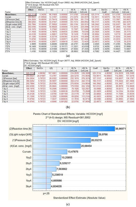
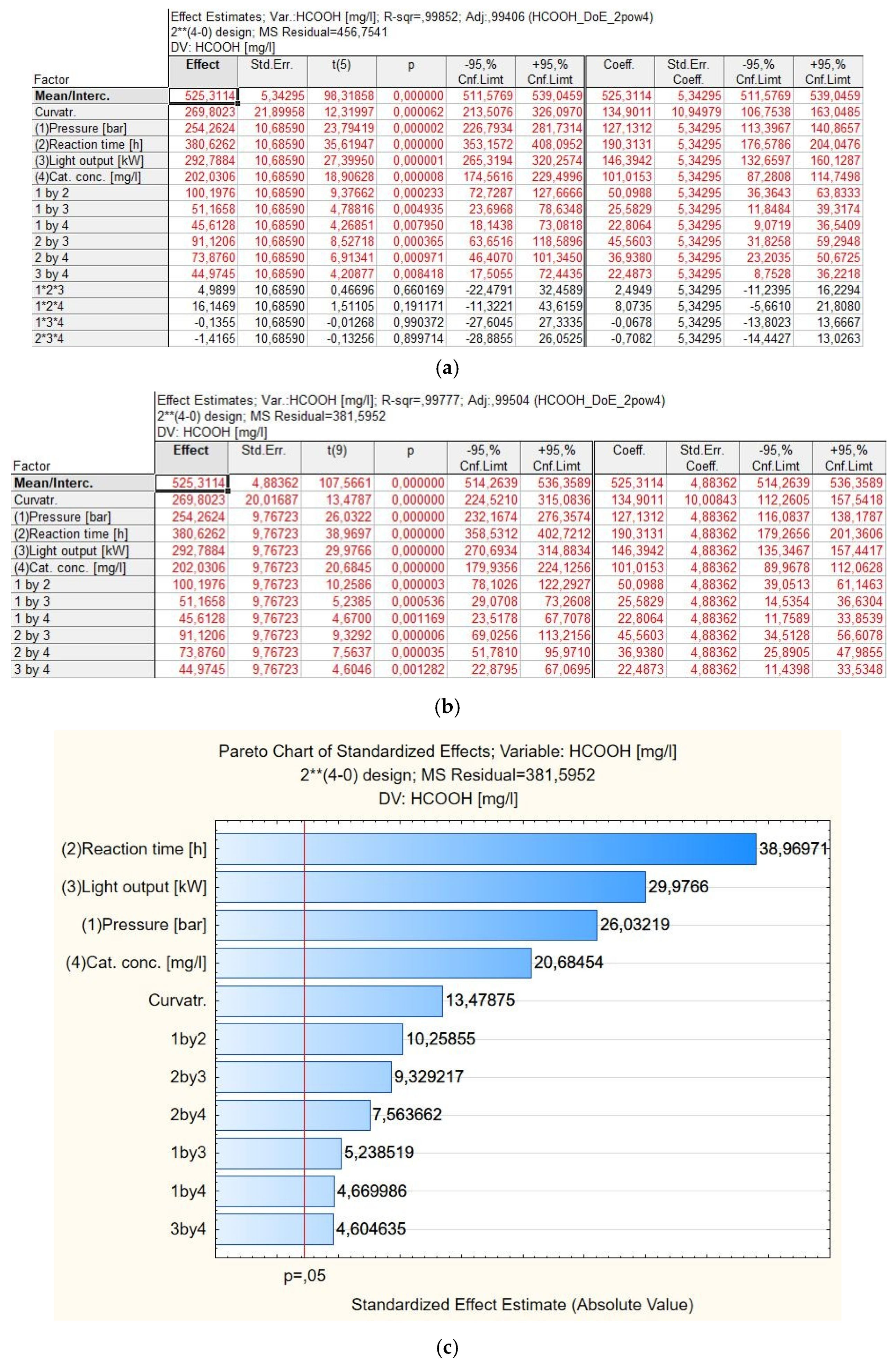
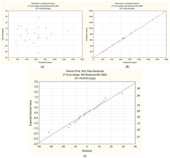
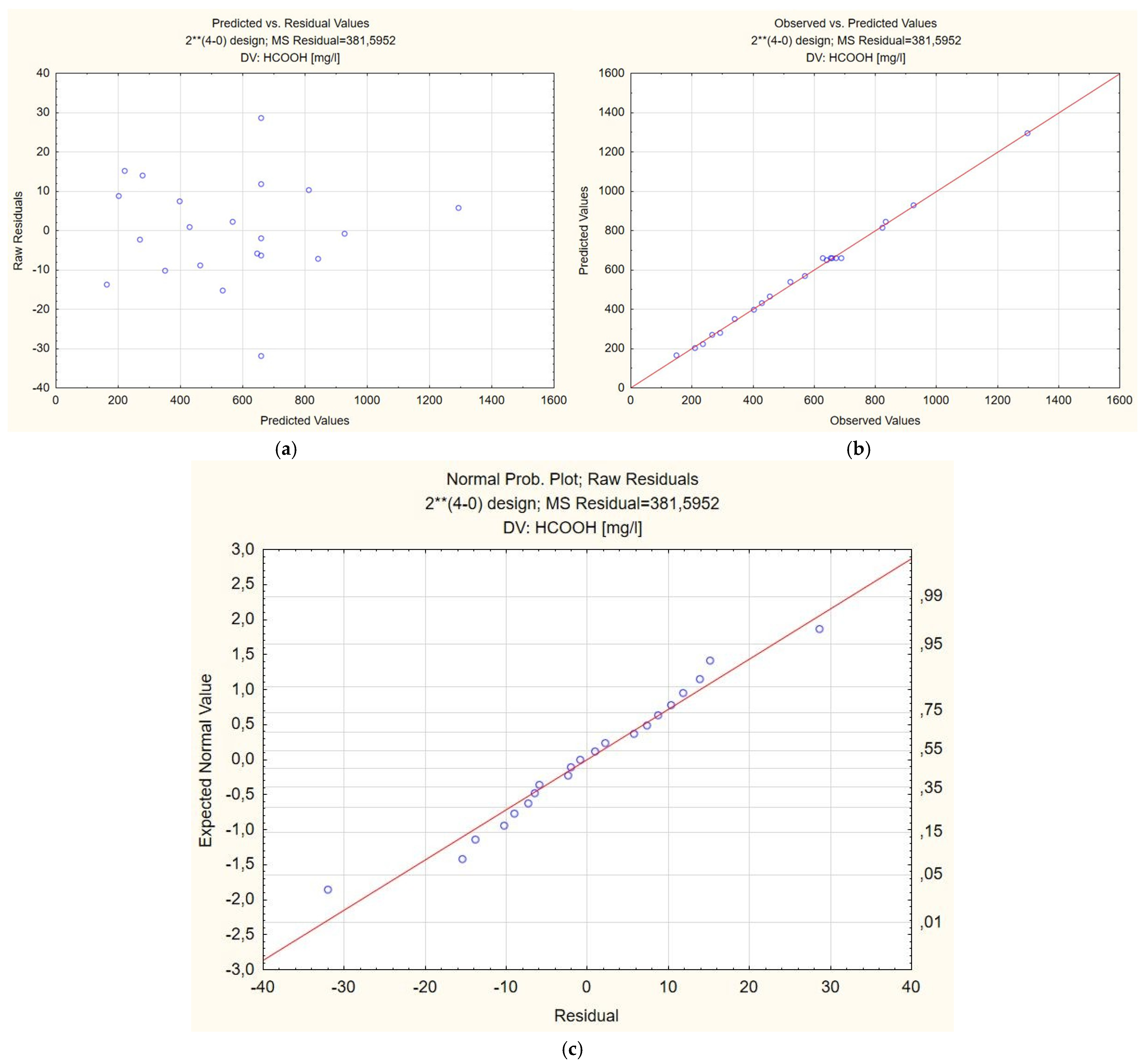
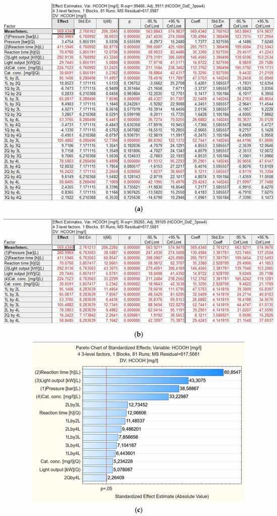
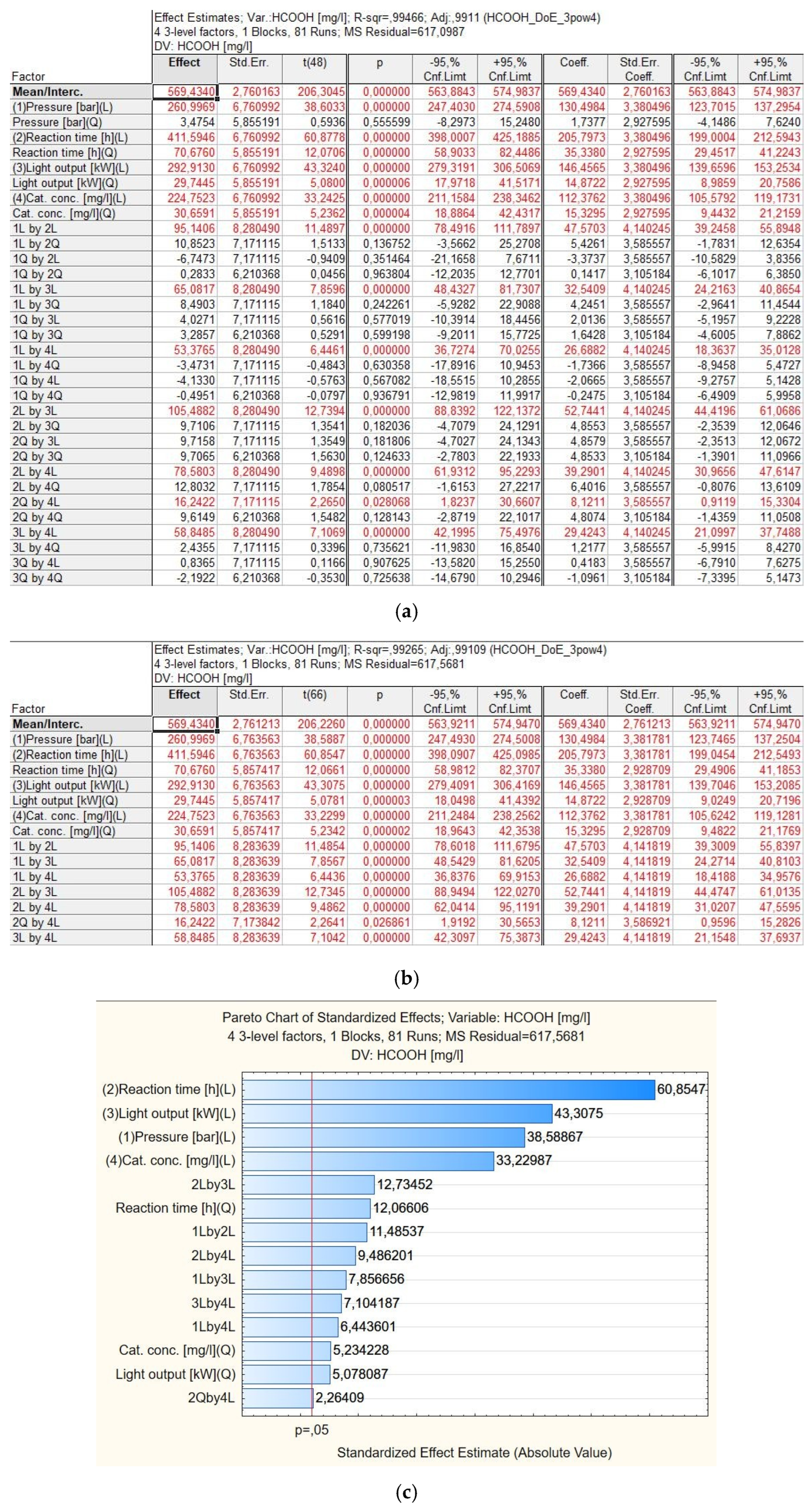
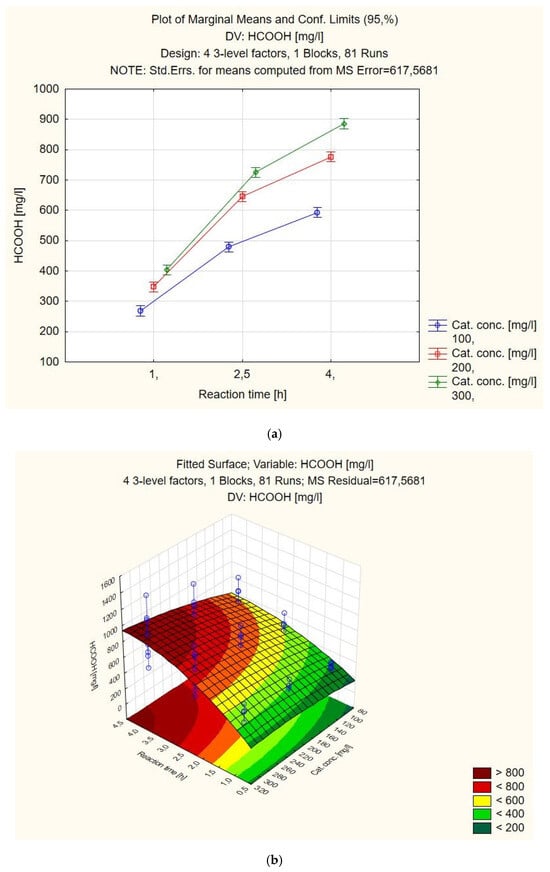
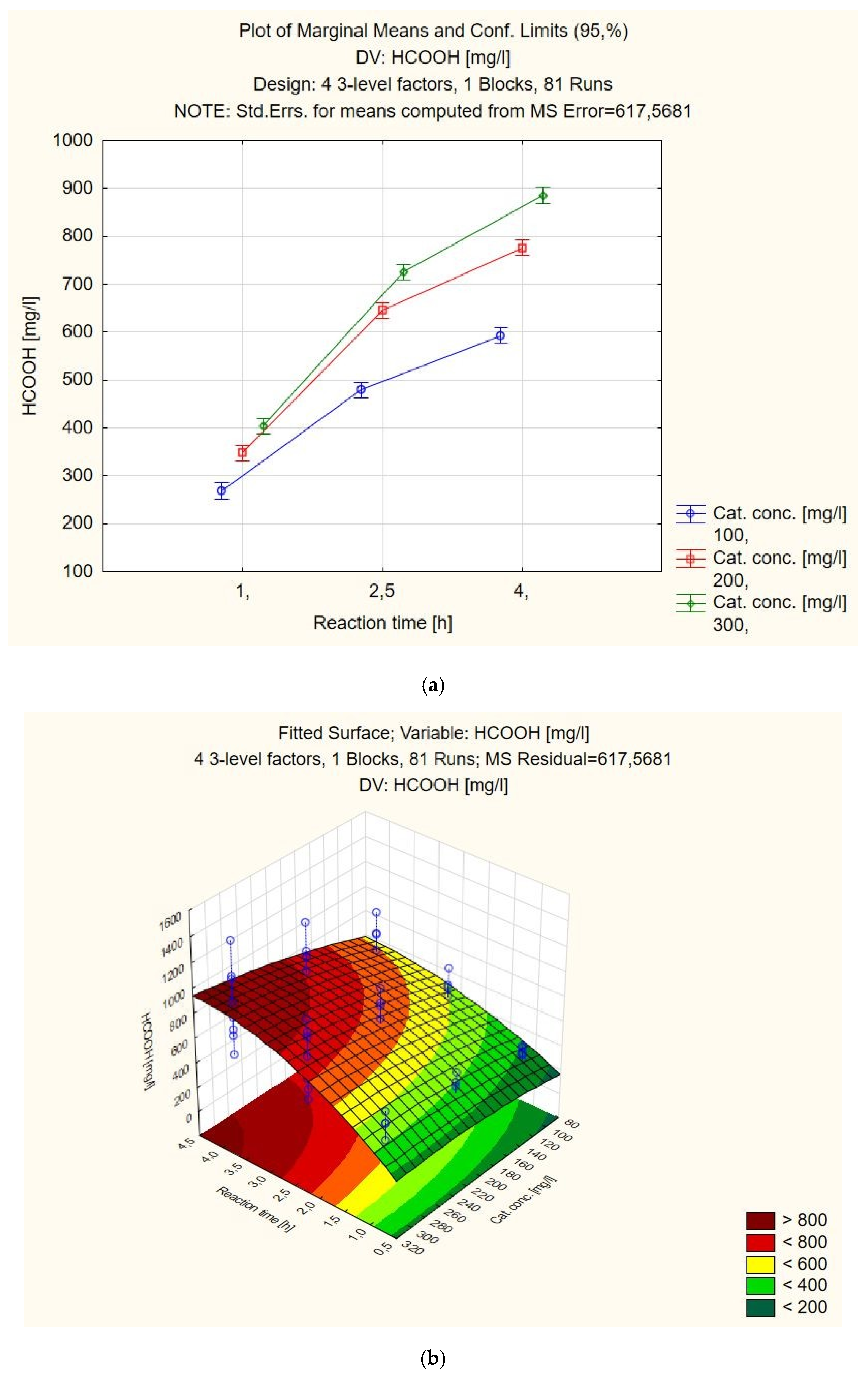
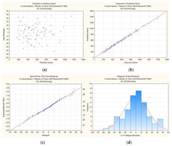
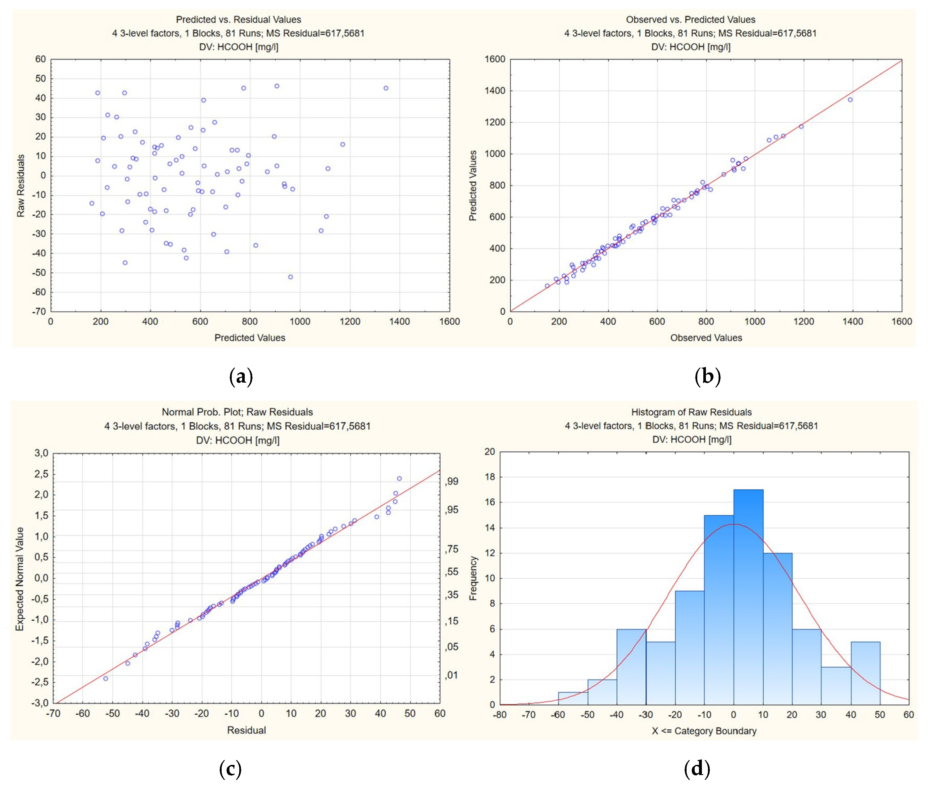
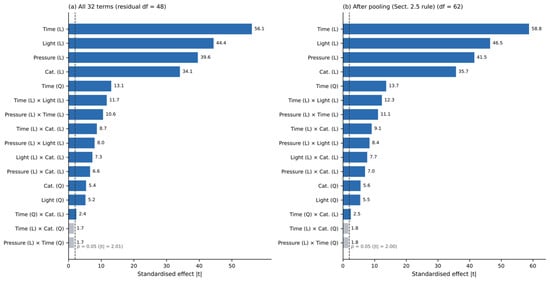
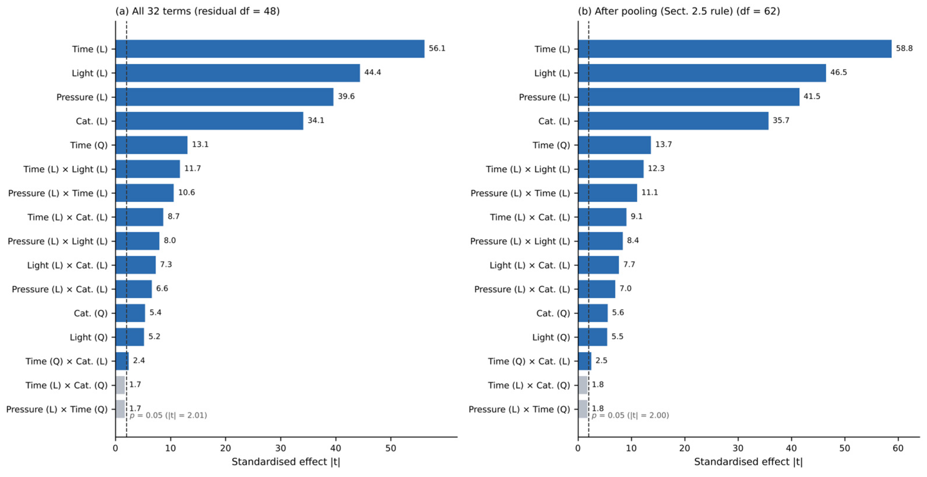

Disclaimer/Publisher’s Note: The statements, opinions and data contained in all publications are solely those of the individual author(s) and contributor(s) and not of MDPI and/or the editor(s). MDPI and/or the editor(s) disclaim responsibility for any injury to people or property resulting from any ideas, methods, instructions or products referred to in the content. |
© 2026 by the authors. Licensee MDPI, Basel, Switzerland. This article is an open access article distributed under the terms and conditions of the Creative Commons Attribution (CC BY) license.