


Abstract
The mid-infrared (MIR) response of cassava leaves (Manihot esculenta Crantz) at different ontogenetic stages and during postharvest deterioration was studied. For this, Fourier-transform mid-infrared spectroscopy (FT-MIR; 4000–600 cm−1) was used to identify spectral signatures and indices as spectral indicators of leaf development and physiological status. Cassava’s HMC-1 variety was used as the model. Spectral signatures were obtained from leaves at two phenological stages (4 and 6 months after planting) using FT-MIR spectroscopy with an attenuated total reflectance (ATR) accessory. A set of classical and experimental spectral indices based on contrast relationships were evaluated, and their discriminatory power across ontogeny was assessed using ANOVA/Kruskal–Wallis and post hoc tests. Postharvest deterioration effects were examined through postharvest monitoring (1–20 days), with temporal, ontogenetic, and interaction effects validated using linear mixed models (LMM), while multivariate structure and spectral convergence were explored via principal component analysis and hierarchical clustering (PCA-HCA). Functionally enhanced derivative spectroscopy (FEDS) was applied as a derivative-based spectral enhancement approach of FT-MIR; in addition, comparative analysis and spectral correlation mapping allowed signals’ selective enhancement and their association with structural molecular components. FEDS-based signal ratios (e.g., 3400/2920 and 1710/1640 cm−1) showed an adequate differentiation of mature leaves and were consistent with spectral changes commonly associated with tissue hydration and cuticular ester-related components. FT-MIR indices showed higher sensitivity to mature stages compared to other ontogenies. It is concluded that FEDS-improved FT-MIR allows the construction of consistent spectral signatures and an enhanced extraction of indices with potential as discriminatory spectral indicators of leaf maturation and postharvest deterioration in cassava.
1. Introduction
Cassava, yuca root, manioc, or tapioca root (Manihot esculenta Crantz) is an important crop in tropical and subtropical zones due to its role in food security and small- and large-scale rural economies [1,2,3]. Cassava’s roots are an important source of carbohydrates, constituting a food source for more than 800 million people, mainly in Africa (Nigeria, Democratic Republic of the Congo, Ghana, among others), Asia (Thailand, Indonesia, Vietnam, India, China, among others), and Latin America (Brazil, Colombia, Paraguay, Venezuela, Ecuador, among others). Even in the United States of America, consumption of this tuber is in the order of 1.9 million tons/year (8% of world consumption) [4]. Moreover, due to its adaptability to adverse conditions, it becomes a strategic opportunity when facing new circumstances emerging from climate change and pressures on production systems as a result [5]. In the Latin American context, Brazil is the main producer, followed by Colombia, representing an important segment in terms of agricultural production, which is destined for direct consumption, but also as a source of raw material to produce starch, bioethanol, and thickener in the food industry [6,7,8,9,10]. From a geographical Colombian perspective, the departments of Bolívar, Córdoba, Sucre, and Magdalena in the Caribbean region have been consolidated as one of the most important areas for cassava cultivation, both in traditional and agro-industrial systems [11].
At present, cassava production faces several limitations due to external factors that significantly impact its yield and quality. These include environmental variability, genetic heterogeneity, and genotype × environment interactions, among others [12,13,14]. In this context, the development of descriptive and predictive technological tools for chemical and agronomic analyses, based on data science and artificial intelligence, is becoming increasingly relevant. In addition, these analytical approaches are characterized by enabling, in many cases, rapid, non-destructive, and real-time monitoring of plant physiological statuses and crop yields. From a practical perspective, having analytical methods with these characteristics is particularly important for crops geared towards food security, sustainability, small-scale farming, and efficiency in production systems based on a circular economy and precision agriculture [15,16,17,18,19,20].
Today, it is well known that advances in miniaturization, cost reduction, and greater accessibility to information technologies have greatly facilitated the ability to acquire and analyze large datasets. As a result, the limitations of many technologies in their adaptability to small-scale production systems are gradually disappearing. Specifically in agriculture, this has meant enormous development in agricultural technology, notably in multi- and hyperspectral analysis of vegetation for the physiological and biochemical characterization of crops [21,22]. In this context, a spectral biomarker (SpBM) can be defined as a quantitative and/or qualitative descriptor of one or more optical responses resulting from the interaction between electromagnetic radiation and plant tissues. Thus, a SpBM provides information that can be used from both technological and practical perspectives, as they are associated with structural, biochemical, and functional properties of plants [23,24,25,26]. Thus, a SpBM is operatively defined as a specific spectral signature or index derived from mathematical combinations of two or more specific wavelengths. The most common indices allow inferences about physiological variables such as chlorophyll content, hydration status, and the presence of phenolic compounds, among others, and are usually based on the UV–VIS–NIR spectrum. On the other hand, FT-MIR-based spectral indices are typically based on the ratio of absorption areas or maxima of characteristic bands associated with specific functional groups, and their spectral signatures are of limited use. These spectra have the disadvantage of exhibiting significant overlap, which hinders the identification of absorption maxima and causes poor differentiation as the compositional and structural complexity of the sample under analysis increases. Furthermore, these spectra often show a strong dependence on sample pretreatment operations such as drying and milling [27,28,29,30,31].
Among the infrared-based spectral indices (or bands) is the lignin index (~1510/~1375 or ~1510/~1030), which has been used to estimate lignin content relative to carbohydrate content by using signals at ~1510 cm−1 (lignin) and ~1375 cm−1 (cellulose), or ~1030 cm−1 associated with polysaccharides [32,33]. Likewise, other SpBMs include the polysaccharide index (~1030/~1510 or ~1150/~897), which has been used as an indicator of cell wall cellulose content by comparing the signals at ~1030 cm−1 (polysaccharides) or ~1150 cm−1 (cellulose) to the signals at ~1510 cm−1 (cellulose) or ~897 cm−1 (β-glucosidic) [34,35,36]; the water index (~3400/~1640), which has been used to assess leaf water content from ~3400 cm−1 (O-H) and ~1640 cm−1 (water) [37,38,39]; and the protein index (~1650/~1540), which has been proposed to assess protein content and metabolism from ~1650 cm−1 (C=O of amide I) and ~1540 cm−1 (amide II) [40].
Despite advances in the development of SpBMs, including spectral signatures and indices, significant limitations remain and restrict their applicability and generalizability. First, many spectral indices exhibit redundancy and saturation effects, especially in high-biomass systems, which limit their discriminatory power. Second, since these analyses are generally performed in situ, spectral responses are strongly influenced by environmental conditions and multiple external factors, such as climate, soil type, water stress, and agronomic practices. Consequently, this environmental dependence introduces high variability, making it difficult to extrapolate models to different contexts [41,42]. Furthermore, at the data level, substantial spectral overlap has been reported, which is an inherent feature in FT-MIR of complex samples. Some examples include different vegetation covers, intrinsic heterogeneity of plants, and differences in physiological states [42,43]. To address these limitations and improve classification performance several approaches have been proposed, including the use of new or combined indices [41,42], data transformation techniques (e.g., decorrelation stretching and contrast enhancement) [43], the implementation of spectral reconstruction algorithms based on machine learning and artificial intelligence [44], multivariate and chemometric analyses [45], and spectral transformations for optimal feature selection (e.g., derived spectroscopy) [46], among others. Another important limitation is the dependence of spectral indices on the measurement scale and spatial resolution of the sensor. While satellite sensors allow for large-scale monitoring, their resolution is often insufficient to capture variability at the level of individual leaves or plants. In contrast, laboratory spectroscopic techniques under controlled and stable conditions, as well as proximal detection approaches, provide higher resolution, but at the cost of reduced spatial coverage and higher operating costs [47,48].
However, a need still exists in relation to improving the sensitivity, specificity, and generalizability of SpBMs; mainly those based on FT-MIR spectroscopy. To address this challenge, this study proposes the use of a spectral deconvolution technique known as Functionally Enhanced Derivative Spectroscopy (FEDS), which involves transforming the spectral response by using a derivative-based function to produce an improved spectrum in terms of resolution of absorbance maxima [49,50]. By FEDS, two types of signals can be identified: primary or legacy FEDS signals, which correlate with the relative maxima of the spectral function, and secondary or “pure” FEDS signals, which appear from the transformation itself. The advantages of this technique include the removal of irrelevant information (i.e., points not associated with relative maxima or minima), increased spectral resolution of overlapping signals, the extraction of hidden or low-intensity spectral features, and ease of data processing, programming, and automation. However, its limitations include sensitivity to noise and dependence on measurement reproducibility, requiring the implementation of appropriate methodological strategies to minimize these effects. Such strategies should be applied both during data acquisition (e.g., managing replications, establishing minimum standard conditions, avoiding stray radiation) and during data processing (e.g., smoothing, normalization, and selecting spectral windows). Despite these limitations, FEDS has been proven effective in the analysis of complex systems such as animal tissues, food products, agricultural materials, soils, and microbial biofilms [47,48,49,50,51,52].
The objective of this study was to characterize the spectral response of cassava leaves at different ontogenetic stages and under conditions of postharvest deterioration, implementing FEDS/FT-MIR spectroscopy in the construction of spectral signatures and indices with potential applications as SpBMs of leaf development and plant physiological status.
2. Materials and Methods
2.1. Experimental Location
The experimental setup and sampling were carried out in the Mindtech S.A.S. experimental agriculture unit, located in a peri-urban area of the California sector, Montería, Córdoba (Colombia), at 8°47′18.8″ N and 75°50′33.5″ W. The region is characterized by a warm tropical climate, with a mean annual temperature of approximately 28 °C and an average annual precipitation ranging between 1200 and 1500 mm, according to the Institute of Hydrology, Meteorology, and Environmental Studies of Colombia [53]. In this study, leaf samples were collected from cassava plants of the HMC-1 variety (ICA-Armenia, Colombia), a clone developed by the International Center for Tropical Agriculture (CIAT, Cali, Colombia) [54,55]. Additional information regarding plant material and cultivation conditions has been previously reported [56].
2.2. Leaf Tissue Sampling, Pretreatment, and Storage
Since spectral characterization of leaf tissue aims to identify physiological and biochemical patterns across developmental stages, only apparently healthy leaves were selected from each biological replicate. Leaf selection was based on morphological and visual criteria, prioritizing leaves with uniform green coloration and no visible signs of spots, deformation, necrosis, chlorosis, or symptoms associated with nutrient deficiencies, abiotic stress, or disease.
Leaf collection was conducted during the morning (08:00–11:00 h) to minimize the influence of midday water stress and excessive transpiration on the spectral measurements. Two phenological stages were evaluated: plants at 4 months after planting, corresponding to the advanced vegetative growth stage, and plants at 6 months after planting, corresponding to the starch accumulation stage. Within each phenological stage, leaves were classified according to their ontogenetic status as: (i) young leaves, fully expanded and located in the upper third of the canopy; (ii) intermediate leaves, located in the upper portion of the middle canopy third; and (iii) mature leaves, located in the lower portion of the middle canopy third.
Immediately after collection, leaves were placed in sealed plastic bags containing a moist cloth to minimize water loss during transport and were transferred to the laboratory within 4 h. Prior to spectral acquisition, leaf surfaces were gently cleaned with absorbent paper to remove dust particles and residual surface moisture.
To evaluate the contribution of tissue microstructure to the spectral response, a subset of mature leaves was dried in a forced-air oven (Digitheat-TFT, J.P. Selecta, Barcelona, Spain) at 40 °C until constant weight and ground using a knife mill (Mikro® UMP, Summit, NJ, USA) to obtain a homogeneous powder (<0.5 mm particle size). Powdered samples were stored in airtight polypropylene containers under dry conditions until analysis. Additional details regarding leaf selection and sampling procedures have been previously reported [56].
2.3. Experimental Design and Dataset Structure
The experimental dataset was organized according to a factorial structure comprising three biological replicates (cassava plants), three leaf ontogenetic stages (young, intermediate, and mature), and two sampling times (4 and 6 months after planting). At each sampling time, three leaves representing each ontogenetic stage were collected from every biological replicate. Spectral measurements were subsequently acquired from both the adaxial (upper) and abaxial (lower) surfaces of each leaf.
The sampling design explicitly distinguished among biological replicates (plants), biological subsamples (leaves), and technical replicates (spectral scans). Individual plants represented the biological level of replication, whereas multiple leaves collected within each ontogenetic category were retained as subsamples to capture within-plant variability. Repeated spectral scans acquired from the same leaf region were averaged prior to statistical analysis and were therefore not treated as independent observations. This hierarchical sampling structure prevented artificial inflation of sample size due to repeated instrumental measurements.
To evaluate whether the sampling time contributed substantially to spectral variability, exploratory PCA and one-way MANOVA were conducted using PC1 and PC2 scores as dependent variables. No significant difference was detected between the spectra acquired at 4 and 6 months (Wilks’ = 0.944, F (2,51) = 1.521, p = 0.228, = 0.056), with an extensive overlap of 95% confidence ellipses in the PCA score plot and no consistent clustering by sampling date in hierarchical analysis (Figure S1). Given the negligible effect size and absence of spectral differentiation, both sampling dates were pooled for subsequent analyses.
The resulting dataset structure for each ontogenetic stage was defined as:
where represents the total number of spectra per ontogenetic stage, () corresponds to the number of biological replicates (plants (n = 3)); () to the number of leaves sampled within each ontogenetic stage (n = 3); (s) to the number of evaluated leaf surfaces (adaxial and abaxial (n = 2)); and (z) to the number of sampling times (n = 2). Based on this sampling structure, 36 spectra were obtained for each ontogenetic category, resulting in a total of 108 spectra per spectroscopic technique after pooling all ontogenetic stages. Instrumental spectral replicates were averaged beforehand and were therefore excluded from these calculations.
Prior to inferential statistical analyses, a systematic spectral characterization and index selection procedure was performed based on the FT-MIR characterization described in Section 3.1, Section 3.2 and Section 3.3, including band assignment, comparison of the adaxial and abaxial leaf surfaces, band-ratio analysis, and spectral correlation analysis. Based on the comparative analysis of both leaf surfaces, only the adaxial surface was retained for subsequent statistical analyses. Spectral indices were first calculated for each individual leaf. Subsequently, the values obtained from the three leaves belonging to the same plant and ontogenetic stage were averaged so that each plant contributed a single observation per ontogenetic stage. Accordingly, the plant was considered an experimental unit in all inferential statistical analyses, including the postharvest linear mixed-effects models. Other details can be found in [56]. The present study extends that framework through FT-MIR measurements and FEDS-based spectral analyses.
2.4. FT-MIR Measurements
MIR measurements were performed using an IRAffinity-1s spectrometer (Shimadzu Co., Kyoto, Japan) equipped with an attenuated total reflectance (ATR) accessory fitted with a ZnSe crystal. Spectra were collected using 16 scans at a spectral resolution of 2.0 cm−1 over the range 4000–600 cm−1.
For each leaf (young, intermediate, and mature), independent MIR spectra were acquired from both the adaxial and abaxial surfaces (three replicates per position). Powdered samples were also analyzed to minimize structural effects and enhance detection of chemical contributions to the spectral response. Additionally, to achieve a detailed characterization of the spectral fingerprint, measurements were collected at specific anatomical regions, including the leaf apex, three points along the leaf blade, the midrib, and the petiole.
2.5. Spectral Data Processing
Spectral data processing included pretreatment, visualization, and feature extraction procedures for subsequent analysis. All processing steps were performed using MATLAB® R2024b (MathWorks Inc., Natick, MA, USA) under an institutional license provided by Universidad del Valle (Cali, Colombia). The main objective was to ensure data quality, reduce instrumental noise, and enhance physiologically and biochemically relevant spectral features.
2.5.1. Data Pretreatment
Data pretreatment was performed to ensure consistent analysis of intrinsic spectral features by reducing noise and standardizing measurement scales. This included smoothing and normalization procedures.
- Smoothing: Prior to normalization, spectra were smoothed to reduce instrumental noise without compromising spectral resolution. Spectral smoothing was performed using the Savitzky–Golay filtering method implemented as a second-order polynomial fit over a moving window of 9 data points [57,58,59]. The Savitzky–Golay smoothing method is based on fitting a polynomial of degree to a moving window of consecutive data points using a least-squares approach. For each central point , the smoothed value is calculated as follows:where are the original values of the signal, and are the deconvolution coefficients calculated as a function of the polynomial order and the window size [57,58,59].
- Normalization: After smoothing, a min–max normalization was applied to rescale spectra to the range [0,1], according to:where is the normalized and scaled absorbance, and is the absorbance at one wavelength [58,60].
2.5.2. Spectral Segmentation
To focus the analysis on physiologically and biochemically relevant regions and avoid masking of subtle variations by dominant signals, spectra were segmented into specific analysis windows (see Table 1). The delineation of these spectral regions enabled a more precise identification of characteristic bands associated with phenolic compounds, photosynthetic pigments, and structural components of the leaf. This approach provided a basis for subsequent signal transformations, as well as comparative and statistical analyses [61,62,63].
Table 1.
Details about spectral segmentation used in this study for FT-MIR.
2.6. Application of FEDS for the Identification of Characteristic Signals
The FEDS transformation was then applied to the normalized spectra. The FEDS formulation combines three operations: inversion, differentiation, and power-law scaling. The inverse transformation enhances contrast in low-intensity spectral regions, allowing weak absorption features to become more pronounced. The derivative operator emphasizes local spectral gradients, which are associated with subtle biochemical transitions between functional groups. However, both inversion and differentiation inherently amplify high-frequency noise. To mitigate this effect, a Savitzky–Golay smoothing filter was applied prior to FEDS computation, ensuring local polynomial continuity and reducing stochastic fluctuations while preserving spectral shape [49,63].
The working equation for the FEDS transform is given by:
where represents the FEDS intensity at a given wavenumber , denotes the first-order derivative of with respect to , and acts as an amplification factor preserving the contribution of the original signal intensity. The parameter controls the nonlinear sensitivity of the transformation by regulating the exponent applied to the inverse-derivative term. In this study, a value of was used for all FTIR datasets. This configuration provides a balance between feature enhancement and noise suppression. The selection of α = 1.7 was further supported by a visual benchmark against the Savitzky–Golay second derivative (Supplementary Figures S4–S6), where FEDS produced sharper and more localized spectral responses for major absorption bands without introducing substantial distortions in the spectral profile [63].
2.7. FEDS-Derived Spectral Indices
Spectral indices were constructed from characteristic FT-MIR bands identified through the FEDS transformation. Candidate bands were selected based on regions exhibiting contrasting spectral responses, supported by comparative spectral analysis and multiregional correlation patterns, as well as their association with specific molecular vibration regions. The selected bands were combined as simple band ratios according to:
where () and () represent the FEDS intensities at the selected wavenumbers (n) and (m), respectively. These indices were designed to emphasize relative differences between spectral regions exhibiting contrasting responses during leaf development and postharvest deterioration.
The FT-MIR indices evaluated in this study are summarized in Table 2. The band notation (υ1–υ15) corresponds to the characteristic FEDS signals described in the spectral characterization in Section 3.1.
Table 2.
Definition of FEDS-derived FT-MIR indices.
2.8. Data Analysis
2.8.1. Analysis of Spectral Data Correlations
To study possible relationships and common patterns between the different spectral regions, correlation matrices were obtained based on Pearson’s correlation coefficient () as the base metric (the subscripts 1 and 2 denote the wavelengths that define the analysis window). This approach allowed us to explore the degree of linear association between the signals at different wavelengths () and to identify dependencies between spectral bands [64]. The coefficients obtained were represented in a correlation map for the two-dimensional identification of the pairs of bands with the greatest and least codependence. Subsequently, the difference in the values of the characteristic signals () was used as the base metric for evaluating the magnitude of change in codependence in the selected band pairs, described as follows:
where is the between wavelengths and in group A (e.g., young leaves), and is the between the same wavelengths in group B (e.g., mature leaves).
The statistical significance of this measure was assessed by applying 10,000 random permutations of the spectral replicates, generating relabeled matrices with samples of different classifications (, , …). This approach allowed the construction of a null distribution of correlation differences under the hypothesis of no effect between groups. Probability values () were estimated as the proportion of permutations in which the absolute value of exceeded the absolute value of the observed (). Differences were considered statistically significant when -value < 0.05.
2.8.2. Analysis of Variance
To evaluate whether spectral differences among ontogenetic stages were statistically significant, mean comparison tests were applied to spectral indices. When assumptions of normality and homoscedasticity were met, one-way ANOVA was performed [65,66]. Otherwise, nonparametric alternatives such as the Kruskal–Wallis’s test were used [67,68]. Post hoc comparisons were conducted using Tukey’s HSD test; when variance homogeneity was not satisfied, the Games–Howell test was applied as an alternative [68].
2.9. Postharvest Deterioration Experiments
To evaluate how spectral signatures respond to temporal changes during postharvest storage, a controlled postharvest deterioration experiment was conducted on previously characterized leaves. This approach aimed to decouple the ontogenetic effects from changes associated with tissue degradation.
After initial spectral acquisition corresponding to the fresh physiological state (), leaves were pretreated and individually labeled. Spectral measurements were performed daily during the first four days (, , , and ) to capture early dehydration and structural changes. Subsequently, measurements were conducted at longer intervals (days 6, 8, 10, and 16 denoted as , , , and , respectively) to evaluate advanced degradation stages.
Postharvest deterioration data were analyzed using linear mixed-effects models (LMMs) implemented in MATLAB® R2024b (fitlme function) [69]. For the linear mixed-effects analysis, spectral indices obtained from the three leaves representing each ontogenetic stage within the same plant were averaged before model fitting. Consequently, the plant was considered the experimental unit, whereas the individual leaves were treated as biological subsamples to reduce within-plant variability. For each spectral index, the model included Day (8 levels) and Ontogeny (3 levels) as fixed effects. Where the data structure permitted full-rank estimation, the Day × Ontogeny interaction was also included as a fixed effect; otherwise, an additive model was fitted:
In this model, Replicate represents the repeated measurements corresponding to a given plant × ontogenetic stage combination across the eight postharvest sampling times. Thus, each replicate corresponds to the average spectral index value for one plant at a given ontogenetic stage. The random intercept (1|Replicate) accounts for the correlation among repeated measurements obtained from the same plant × ontogenetic stage combination over time. A total of 72 observations were included in the analysis (3 plants × 3 ontogenetic stages × 8 time points). Statistical significance was evaluated at the 95% confidence level. Complete model outputs, including fixed-effect estimates, interaction terms where estimable, and goodness-of-fit statistics (AIC, BIC, R2 marginal), are provided in Supplementary Table S2.
The joint effects of ontogeny and postharvest deterioration were further explored using principal component analysis (PCA) [70] and hierarchical cluster analysis (HCA) [71].
3. Results and Discussion
3.1. Spectral Fingerprint of Cassava Leaf Tissue by FT-MIR
Figure 1 shows the average and unmodified FT-MIR spectra of intact leaf tissue (FT0-y) and powdered dry leaf tissue (PDM-y) (dashed red and black lines, respectively). Also, their respective signal assignments are shown (Table 3). The usefulness of FEDS in spectral resolution is reflected in the splitting of signals between 4000 and 2400 cm−1. In this region, FT-MIR shows a strong overlap of signals that makes it difficult to differentiate the contributions; however, in the FEDS spectrum, the resolution improves significantly.
Figure 1.
Spectra of FT-MIR and FEDS of TF0-y and PDM-y.
Table 3.
FT-MIR/FEDS band assignments and spectral shifts in cassava leaf tissue: intact (TF0-y) versus powdered, dry milled (PDM-y) samples.
Between 3400 and 3200 cm−1, both TF0-y and PDM-y exhibit broad, asymmetric bands with fluctuations along the spectral line, suggesting that the observed band in each case results from the overlap of contributing or hidden bands. Vibrations associated with -OH groups (e.g., hydroxyl groups, carboxylic acids) and -NH groups (e.g., amines, amides) are expected in this region. These may be present in the structure of various molecular components of leaves. Thus, FEDS shows that, in this region, the TF0-y spectrum has at least four contributions, identified by the positions υ1, υ2, υ2*, and υ2**. In addition, the intensities of these signals follow the order υ1 > υ2 > υ2* > υ2**.
In contrast, these four signals can also be identified using FEDS in the PDM-y spectrum, but a different order is observed: υ2 > υ1 > υ2* > υ2**. Because TF0-y can be described as the initial state for obtaining PDM-y (i.e., TF0-y → PDM-y + H2O + others), it is possible to support the assignment of signals to the changes expected due to water loss. Thus, as the water content decreases, the vibrations associated with hydration O-H bonds decrease, and the relative proportion of O-H bonds associated with other organic molecular structures increases. Therefore, the contribution of O-H bonds is smaller, and the band shifts to the left (higher vibration frequencies). From this, it can be concluded that υ1 corresponds to vibrational contributions from water molecules contained in the leaves, while υ2 corresponds to O-H vibrations from non-carboxylic organic molecules (e.g., polysaccharides). On the other hand, υ2* can be associated with the O-H bonds of -COOH groups (carboxylic acids), and υ2** is associated with -NH groups of amines or amides, since, due to the greater electronegativity of oxygen, N-H vibrations are expected at lower frequencies [72].
On the other hand, the signals identified as υ2*AC1 and υ2*AC2 are associated with O-H stretching vibrations in carboxylic acids that form structures with strong hydrogen bonds. These can be, for example, the result of hydrogen bonds between the O-H from -COOH attached to aromatic rings [73], or between these and water molecules. These are very likely to be found as part of the lignocellulosic material of leaves. Similarly, the loss of water would lead to a decrease in this type of interaction with the consequent shift to higher frequencies, which, in the spectra, would be evidenced as a shift from υ2*AC2 to υ2*AC1 considering the change TF0-y → PDM-y.
The bands corresponding to the stretching vibrations of aliphatic C–H groups (υ3 and υ4 at 2920, 2860) were consistent and stable in their spectral position. Conversely, the ester carbonyl signal (υ5 at 1716 cm−1) displayed an exact frequency match in both samples, albeit with a significant reduction in its relative intensity in PDM-y. This decrease could be attributed to the partial disruption of the cuticular layer, whose cutin polymeric matrix concentrates the highest proportion of surface ester groups [74]. In the 1650–1630 cm−1 region (υ6), stretching vibrations of the C=O group characteristic of amides (CONH)—commonly known as the Amide I band—are present. This signal is associated with structural proteins and is typically overlapped with carbohydrate C=O vibrations and the water-bending (scissoring) band in this same region [61]. This feature is highly correlated with the band located between 1560 and 1520 cm−1 (υ7), which arises from N–H bending vibrations coupled with C–N stretching vibrations, known as the Amide II band. Both bands reflected a constant and equivalent υ6/υ7 intensity ratio, indicating that the proportionality between both tissue types is preserved, although slight shifts toward higher frequencies were observed in TF0-y, likely associated with a higher degree of hydration and structural organization of the proteins [61]. On the contrary, the υ5/υ6 intensity ratio evidenced a relative decrease in the intensity of ester carbonyl groups relative to amide carbonyls (υ5/υ6 < 1) in PDM-y. This indicates a greater exposure of structural proteins and a lower contribution of cutin esters from the cuticular layer following the physical changes induced in the sample. Within the 1400–1000 cm−1 range (υ8\υ13), the main contributions stem from C–O and C–O–C bonds of structural polysaccharides such as cellulose, hemicellulose, and pectin (υ8, υ9, υ11, υ12). In this region, a higher band intensity was observed in TF0-y compared to PDM-y [75].
At lower wavenumbers, FT-MIR spectra allow the identification of signals because, although they overlap, their absorption maxima are clearly distinguishable. However, two exceptions can be identified. These correspond to signals υ12 and υ14, which do not appear fully defined in both FT-MIR spectra. The υ12 signal (1075–1135 cm−1) may be associated with C-O vibrations of alcohols, acids, and cyclic ethers; therefore, its origin can be varied. However, contributions from aryl-O-alkyl ether characteristic bonds of lignin are also expected in this region [76]. Likewise, the υ14 signal (780–820 cm−1) may be associated with the deformation of carboxylate groups and out-of-plane vibrations of aromatic rings of guaiacyl and sinapyl units of lignin [76]. Regardless of the stage of leaf development, lignin contents in cassava leaves have been reported to range from 0.9 to 8.4 g/100 g of dry matter (DM), with the lower limit (0.9 g/100 g DM) representing the characteristic average value for very young leaves, whereas the upper limit (8.4 g/100 g DM) corresponds to the characteristic average content of mature leaves [77]. In contrast, the crude protein content of mature cassava leaves is typically around 19.7 g/100 g DM [77], while values reported across different cassava cultivars range from 17.7 to 38.1 g/100 g DM [78]. These leaves contain aromatic amino acids such as phenylalanine (5.4 g/100 g protein) and tyrosine (2.8–4.0 g/100 g protein) [78]. However, since these amino acids are present in relatively small quantities, their contribution is not expected to be significant, and consequently, these signals can be considered characteristic of lignin. Furthermore, proteins are found within the cell structure, while lignin, cellulose, and hemicellulose form part of the external cell structure [78,79].
3.2. Analysis of FT-MIR Spectral Signatures as a Function of Leaf Ontogeny
Based on the FT-MIR characterization of the leaves, the ontogenetic effect on the spectral response was evaluated. Figure 2 shows comparisons of the FT-MIR spectra of cassava leaves for the different developmental stages studied and for each of the surfaces (adaxial and abaxial).
Figure 2.
FT-MIR spectral fingerprint of cassava leaves at different stages of growth: Young leaves (red dash line), intermediate leaves (blue dash line), and mature leaves (orange dash line) for both leaf surfaces (adaxial and abaxial), in three spectral regions: MIR1 (4000–2800 cm−1), MIR2 (1800–1300 cm−1), and MIR3 (1300–600 cm−1). Reproducibility analysis (standard deviation) of FT-MIR spectra and FEDS is shown in each case.
As expected, Figure 2 shows that the fundamental chemical composition is relatively constant during the stages of leaf development. However, systematic variations are observed in the intensity ratio of some bands, suggesting that spectral information can provide data on the degree of leaf maturity. A detailed analysis is presented below:
In the MIR1 region, the υ1/υ3 ratio (3400/2920) was identified, which showed a decreasing trend with the progression of leaf development on both leaf surfaces. This trend reflects a decrease in hydroxyl groups (υ1) compared to aliphatic groups (υ3), suggesting changes toward reduced hydrophilicity in mature leaves. This is consistent with the increased wax composition, especially in the cuticular zone of the leaves [79,80]. The described trend is clearly observed in the box and whisker plots shown in Figure 3, which demonstrate that on the adaxial surface, the υ1/υ3 values in mature leaves are distinct from, but do not overlap with those of young and intermediate leaves. In contrast, on the abaxial surface, the ranges of the three ontogenetic stages overlap. Consequently, it was established that changes associated with maturity and the relative proportion of OH/(CH2, CH3) groups can be detected mainly on the adaxial face.
Figure 3.
Box and whisker plot explaining the variation in the spectral ratios υ1/υ3 and υ5/υ6: Variation in the spectral ratios as a function of the development stage ((A1) and (A3) correspond to the adaxial face, while (A2) and (A4) correspond to the abaxial face); and variation in the spectral ratios as a function of the adaxial and abaxial face ((A3) and (A4) correspond to the spectral ratios υ1/υ3 and υ5/υ6, respectively).
In the MIR2 region (Figure 2), the υ5/υ6 ratio (1716/1640) increases progressively with leaf maturity, particularly on the adaxial surface. In contrast, young leaves exhibit the opposite behavior, with a greater relative contribution from the υ6 band. This is consistent with the accumulation of esterified compounds primarily associated with cuticle thickening and maturation, and the reduction in soluble proteins and metabolically active compounds [80,81].
On the other hand, the standard deviation on both leaf surfaces, for each developmental stage, showed less intrasample variability on the abaxial surface compared to the adaxial surface across all spectral ranges (see Figure 3). Since the spectrum reflects, to some extent, the nature of the functional groups contained in the sample, it can be inferred that the abaxial surface had a more uniform composition. However, the adaxial surface showed greater heterogeneity, possibly associated with variations in the thickness, continuity, and composition of the cuticular layer. In conclusion, the results suggest that the adaxial surface is more sensitive to the structural and chemical changes associated with the leaf maturation process, while the abaxial surface maintains a more stable behavior without providing much useful information for ontogenetic discrimination.
3.3. Correlational Analysis Based on Pearson Coefficients
3.3.1. Correlative Dynamics for the FT-MIR Spectra
Figure 4 shows the correlation maps for young, intermediate, and mature leaves in the segmented spectral regions of FT-MIR spectra. The correlation maps described in Figure 4A reveal a progressive increase in collinearity as tissue maturation advances. In young leaves, correlations between bands show a heterogeneous pattern, consistent with tissue undergoing active structural and biochemical differentiation. In intermediate stages, this pattern begins to consolidate, and finally, in mature leaves, a continuous block of high-magnitude positive correlations appears, particularly in the MIR3 region (≈600–900 ). This increase in collinearity in mature leaves suggests greater functional integration of the tissue.
Figure 4.
FT-MIR spectral correlation maps for: (A) young, intermediate and mature leaves from bands selected by FEDS (υ1–υ15) and (B) between ontogenetic groups.
Figure 4B shows differential correlation maps between the different stages of leaf development. These maps allowed for the identification of key functional transitions. Comparisons reveal more pronounced spectral reorganization patterns between young and intermediate leaves. In contrast, the differences between intermediate and mature leaves are less marked and are concentrated in specific regions, suggesting a progressive stabilization of the spectral organization in mature tissues. Representative band pairs displaying the largest positive and negative Δr values are summarized in the Supplementary Figure S3.
The Young–Intermediate transitions were primarily dominated by decreases in the codependence of key band pairs such as υ1/υ3 and υ5/υ6, corresponding to the vibrational relationships between O-H/C-H and C=O(ester)/C=O (Amide I) bonds, respectively. This suggests an initial structural reorganization in which the relative proportion of lipophilic compounds and protein-rich structures changes. This chemical reorganization can be interpreted because of processes such as the progressive thickening of the cuticular layer, the deposition of epicuticular waxes, and the increase in structural polysaccharides.
On the contrary, as leaf maturity occurs, this trend reverses for most band pairs, as the changes in many of these relationships stabilize, consistent with the structural consolidation expected at maturity stages. However, in certain functional domains, the decreasing correlation differences continue, as occurs with υ1 (O–H) and υ3 (C–H), indicating that a decoupling of these two domains persists, which could be associated with the hydrophilic nature of υ1 and the lipophilic nature of υ3. This pattern is consistent with the analysis of the spectral fingerprints in Figure 2 and Figure 3, which show very marked and distinctive intensity relationships on the adaxial surface of mature leaves for these specific bands.
3.3.2. Comparison Between Ontogenetic Groups, Differential Correlation (), and Statistical Significance Using Permutations in FT-MIR
Pairwise differences in Pearson correlation coefficients () between ontogenetic groups were evaluated for statistical significance using a two-tailed permutation test (n = 10,000 permutations). A p-value ≤ 0.05 indicates that the observed is unlikely under the null hypothesis of no group difference in correlation structure. The p-values ≤ 0.05 indicate that the values of are significantly larger than the values obtained through permutations of the input matrices (see Table 4). The pairs of signals with values of Δr showing consistent and significant changes may be candidate spectral markers; consequently, they are candidates for the construction of functional spectral indices and are evaluated by ANOVA to test their discriminative capacity and statistical consistency.
Table 4.
Correlational comparison and permutation test in FT-MIR for the different stages of development.
3.3.3. FEDS-Based FT-MIR Spectral Indices
Post hoc analysis of these indices showed clustering patterns that evidenced progressive transitions, from spectral signatures with a predominance of vibration bands associated with hydrophilic and metabolically active components towards spectral signatures related to a more organized and stable structural matrix (see Table 5, Figure 5 and Supplementary Table S1).
Table 5.
Results of the normality, homogeneity, and ANOVA statistical analysis tests for the classical and experimental spectral FEDS-FT-MIR indices.
Figure 5.
Distribution of mean values ± standard error of classical and experimental spectral indices (post hoc plots), FEDS-based FT-MIR indices in young, intermediate, and mature leaves. Letters indicate significant differences between ontogenetic stages according to the post hoc test (p < 0.05). The red dotted vertical lines indicate the ranges of variation for each index.
The IMIR1 index did not show significantly different values between the ontogenies (p-BH-FDR = 0.109), indicating that the relationship between bands associated with hydroxyl and carbonyl groups is not sufficiently sensitive to the structural and compositional changes in leaf tissue during its development. This is possibly because the relative changes in these bands are proportional and co-evolve in a balanced manner during ontogeny. In contrast, IMIR2, IMIR6, and IMIR7 showed significantly higher values in young leaves compared to mature leaves (IMIR2: p_BH-FDR = 0.024, η2p = 0.40; IMIR6: p_BH-FDR = 0.002, η2p = 0.62; IMIR7: p_BH-FDR = 0.010, η2p = 0.50), while intermediate leaves exhibited spectral responses that overlapped with those of young leaves. This pattern indicates a greater relative contribution of bands associated with hydroxyl groups, bound water, or primary or secondary amino groups in the early stages of leaf development. In particular, the behavior of IMIR2 suggests a higher relative content of water or compounds with O-H and N-H bonds in young leaves, which is consistent with metabolically active tissues and a lower degree of lignification.
IMIR6 and IMIR7 are indices that relate to the Amide I band (1640 cm−1), which is primarily associated with proteins and structural water, and the C-H strain bands of structural polysaccharides. They show a decrease from young leaves toward mature leaves, which may be linked to the relative increase in the formation of structural carbohydrates and other cell wall components in mature leaves [81,82]. Meanwhile, the IMIR3 and IMIR4 indices, which relate the stretching vibration bands of aliphatic C-H bonds (υ3 and υ4) and the Amide I band, showed the opposite pattern with significantly higher values in mature leaves (IMIR3: Kruskal–Wallis, p_BH-FDR = 0.010, ε2 = 0.55; IMIR4: p_BH-FDR < 0.001, η2p = 0.71). This behavior is consistent with the relative increase in aliphatic C-H groups compared to the signals associated with amides and bound water [82]. Furthermore, the IMIR5, IMIR8, and IMIR9 indices showed patterns of differentiation between young and mature leaves, but with a transitional behavior (IMIR5: p_BH-FDR = 0.024, η2p = 0.40; IMIR8: Kruskal–Wallis, p_BH-FDR = 0.002, ε2 = 0.82; IMIR9: p_BH-FDR = 0.002, η2p = 0.64); that is, the intermediate leaves showed an overlap with both extreme groups indicating a progressive change in the three stages evaluated. In the case of IMIR 5, the related bands allow us to infer that the relative proportion of carbonyl bonds of ester groups and the Amide I band progressively increase towards maturity, which is consistent with a progressive accumulation of aliphatic cutin esters as the thickening of the cuticular layer occurs.
Finally, the IMIR10 index showed a clearly distinct behavior from the other FT-MIR indices evaluated (p_BH-FDR = 0.015, η2p = 0.45). It was the only one capable of statistically significantly discriminating between intermediate and mature leaves, while young leaves showed overlap with both ontogenetic groups. This nonlinear pattern suggests that IMIR10 does not respond gradually to leaf development but is especially sensitive to structural processes that consolidate in advanced stages of leaf maturation. The band at 1024 cm−1 is mainly associated with C-O and C-O-C vibrations of polysaccharides, particularly cellulose and pectin, which are fundamental components of the cell wall. In this sense, the spectral differentiation between intermediate and mature leaves can be interpreted as a reflection of the greater organization and rigidity of the cell wall, while in young leaves, the high compositional heterogeneity of the cell wall may lead to greater spectral variability, which would explain the observed statistical overlap.
3.4. Analysis of the Temporal Dynamics of Spectral Indices Through Induced Leaf Degradation Experiments
In this study, temporal analysis was employed as an experimental strategy to identify spectral indices with a high capacity to detect postharvest deterioration processes and to evaluate their suitability as indicators of tissue degradation. Given that measurements were conducted under strictly controlled conditions (lighting, sample interaction, and instrumental noise), the resulting values should not be interpreted as direct evidence of an active physiological state, but rather as a representation of the persistence or progressive deterioration of the tissue’s optical properties associated with temporal degradation of detached leaves maintained under controlled storage conditions.
In this context, the analysis addresses the following question: once the spectral signature of a young, intermediate, or mature leaf has been established, to what extent is it affected by degradative processes associated with storage time?
Figure 6 shows the temporal evolution of the FT-MIR indices (IMIR2, IMIR3, IMIR5, IMIR7, IMIR8, and IMIR10), which exhibited the most significant changes over the observation period. In this context, representative indices are those that showed clear temporal trends and/or that displayed visible ontogenetic differences between young, intermediate, and mature leaves during storage. In general terms, the indices showed differentiated temporal responses according to leaf ontogeny, suggesting that the FT-MIR spectral response reflects chemical and structural changes associated with each stage of development. In addition, this allowed for the observation of defined temporal trajectories with distinct ontogenetic patterns, which are detailed below:
Figure 6.
Temporal evolution of FT-MIR spectral indices throughout the observation cycle (days): IMIR2 (A), IMIR3 (B), IMIR5 (C), IMIR7 (D), IMIR8 (E), and IMIR10 (F). Mean values ± standard deviation are shown for three phenological stages: young, intermediate, and mature. Error bars represent intra-group variability at each sampling date.
The IMIR3 and IMIR5 indices show progressive increases in intermediate and mature leaves, while young leaves maintained low and relatively stable values. From a chemical standpoint, this behavior indicates, in the case of IMIR3, a relative increase in the intensity of the signals associated with aliphatic C-H groups (2920 cm−1) compared to the Amide I band; while, in the case of IMIR5, a relative increase in the intensity of the band associated with C=O groups of esters is observed compared to the same Amide I band. This suggests that the inherent loss of moisture due to the degradation process decreases the spectral contribution associated with the water scissor mode, which overlaps with the amide I band. In contrast, the aliphatic C-H and C=O vibrations of esters are less affected by these changes, so their relative intensity remains more stable, leading to the progressive increase observed in intermediate and mature leaves. In the case of young leaves, this effect is much less pronounced. Its higher water content and still poorly consolidated tissue structure act as a buffer system, attenuating the spectral changes associated with dehydration.
Unlike the other indices, the IMIR2, IMIR7, and IMIR8 indices show a decreasing trend, which is more pronounced in intermediate and mature leaves. This is associated with a gradual decrease in the intensity ratio between the bands υ1/υ3 (3400/2920), υ6/υ9 (1640/1364), and υ15/υ5 (656/1716), respectively. In the case of IMIR2, this is associated with the contrast between OH stretching vibrations and aliphatic C-H stretching vibrations. Therefore, the gradual decrease is consistent with the progressive loss of moisture during degradation. However, this decrease is observed to be attenuated and differentiated in young leaves from the first days of monitoring. In the case of IMIR7, the water imbalance is extrapolated to the amide I band, which, as previously mentioned, has an overlap of the C=O stretching vibration bands of amides and the water scissor bending band. Therefore, the decrease in the ratio can be attributed to the loss of contribution from this band. On the other hand, IMIR8 relates the C-O-C strain vibrations and the C=O stretching vibrations. The decrease in the index in this case suggests that, during postharvest degradation, the relative contribution of C=O groups becomes more dominant, which is consistent with processes of chemical reorganization and relative accumulation of oxygenated compounds in the more developed leaves.
Finally, IMIR10 shows an increasing trend in the three ontogenies, although with differentiated values in young leaves. The mathematical relationship between the bands linked to structural polysaccharides and the amide I band suggests that the index responds mainly to the progressive consolidation of the cell wall, a process that is more clearly manifested in mature leaves.
3.5. Analysis of Spectral Variability in the Face of Ontogenetic and Temporal Factors Using Linear Mixed Models (LMM) and Principal Component Analysis (PCA)
In this stage of the study, the objective was to evaluate which spectral indices were most strongly associated with leaf degradation, and how their sensitivity is modulated by ontogenetic stage and the passage of time. To achieve this, the importance of each index was analyzed in isolation, and how its sensitivity is affected by its stage of maturity (ontogeny) and the passage of time was explored. Given the nature of the data, a sequential approach was chosen that integrates the accuracy of the LMMs with the overall view of PCA.
In the FT-MIR region, LMM results revealed that Day, Ontogeny, and their interaction (Day × Ontogeny) were statistically significant for nine of the ten evaluated indices (p < 0.05; Figure 6). This generalized significance pattern indicates that spectral changes in the MIR region are simultaneously driven by the biochemical composition inherent to each ontogenetic stage and by the temporal dynamics of postharvest deterioration—and that these two effects do not act independently. The only exception was IMIR10, for which only the Ontogeny effect was significant (p = 3.68 × 10⁻⁷), while neither the Day effect (p = 0.553) nor the interaction (p = 0.261) reached significance. This positions IMIR10 as a static discriminator of ontogenetic stage rather than a dynamic sensor of postharvest deterioration (see Figure 7).
Figure 7.
Evaluation of the statistical significance of the factors in the linear mixed model (LMM) for the spectral indices of FT-MIR. The graph shows the significance levels expressed as −log(p-value) for the fixed effects of “Day” (blue), “Ontogeny” (orange), and “Day × Ontogeny Interaction” (yellow). The red dashed horizontal line indicates the critical significance threshold . Red asterisks (*) accompanied by a numerical value indicate indices whose significance exceeds the limit of the plotted scale (>20), indicating an extremely low probability of error ().
The significant Day × Ontogeny interaction across nine indices indicates that temporal deterioration trajectories differ among ontogenetic stages. Mature leaves showed the steepest marginal temporal response in the majority of indices (IMIR1, IMIR3, IMIR4, IMIR5, IMIR6, IMIR8, and IMIR9), while young leaves were most responsive in IMIR2 and IMIR7 (See Supplementary Table S2). This differential sensitivity is consistent with the nature of the signals in the MIR region, where fundamental absorption bands associated with specific molecular vibrations (C–H, O–H, N–H, and C=O) dominate, providing information on the biochemical composition of the leaf and its evolution during ontogenetic development and postharvest degradation.
Among the evaluated indices, IMIR3, IMIR4, and IMIR5 warrant more specific analyses. These indices relate the stretching vibrations of aliphatic groups and C=O groups associated with esters (approximately 2920–2860 cm−1 and 1716 cm−1, respectively) to the υ6 band around 1640 cm−1, which is primarily associated with protein Amide I and overlaps with the scissor bending band of water. It is posited that it is not coincidental that these three indices, which share υ6 as their denominator, exhibit the lowest R2marginal values among the significant indices (0.745–0.777), suggesting that while the fixed effects are statistically significant, the υ6 band introduces additional variability that is not fully captured by the Day + Ontogeny + Day × Ontogeny structure alone. It is highly likely that υ6 extracts spectral information related to dehydration processes and protein conformational reorganizations occurring simultaneously during degradation. The significant Day × Ontogeny interaction further suggests that these processes unfold at different rates depending on the initial physiological state of the leaf tissue. For example, young leaves, with a higher water content, thinner cell walls, and a less consolidated organic matrix, tend to partially dampen spectral changes associated with moisture loss in early storage stages. In contrast, intermediate and mature leaves, with more established tissue organization, may experience a more marked decrease in the υ6 contribution upon dehydration onset, causing temporal effects to be expressed with greater spectral intensity.
It should be noted that the present study was conducted using detached leaves monitored during storage. Therefore, the observed spectral changes may reflect both ontogenetic differences and postharvest physiological processes, including dehydration and tissue degradation. Consequently, the proposed indices should be interpreted as spectral correlates of developmental stage rather than definitive biomarkers of programmed in planta senescence.
3.6. Multivariate Structure and Convergence Trajectories (PCA)
When analyzing the FT-MIR region indices, the variability hierarchy changes markedly in both the long-term (Figure 8) and short-term (Figure 9) scenarios. In both cases, the variability associated with PC1 and PC2 explains more than 70% of the variance, maintaining ontogenetic separation as the dominant axis. In the full monitoring scenario of Figure 8, the ontogenetic signature is highly persistent. Contrasting the total convergence seen previously, time does not erase the original imprint; instead, a temporal drift occurs within the ontogenetic groups. The dendrogram in Figure 8C confirms the ontogenetic hierarchy in a very interesting way, especially in the first days of monitoring. In this case, the formation of an orange cluster is clearly observed, grouping exclusively mature leaves between days 1 and 10, while another cluster clearly segregates young leaves between days 1 and 4. However, a single cluster can be observed that segregates the samples according to the temporal degradation in mature and intermediate leaves after 16 days of monitoring.
Figure 8.
PCA of the FT-MIR spectral indices in 16 days of postharvest monitoring: (A) Projection of the samples on the PC1-PC2 plane to explain the variance for each principal component. (B) Loadings of spectral indices in the first three components. (C) Hierarchical clustering dendrogram based on the PC1-PC2 projections.
Figure 9.
PCA of the FT-MIR spectral indices over 4 days of postharvest monitoring. (A) Projection of the samples on the PC1-PC2 plane to explain the variance for each principal component (note that outliers were not identified). (B) Loadings of the spectral indices on the first three components. (C) Hierarchical clustering dendrogram based on the PC1-PC2 projections.
The above reflects the capacity of the FT-MIR technique to detect changes at the molecular level. Thus, there are indices that extract relationships from sufficiently stable regions of molecular vibration, or that are very strong ontogenetic markers, as has already been demonstrated in previous analyses. This generates a damping effect on some degradative effects that occur over time. In short, the degradation must lead to a chemical change large enough to force a change in the initial ontogenetic signatures. The above can be seen in the loading plot in Figure 8C, which shows that indices such as IMIR9 and IMIR10, which exhibit vibration band relationships primarily of the hydrocarbon skeleton of the leaves, and which, according to the LMM, are indices with a predominance of the ontogenetic effect over the temporal degradation effect, contribute very little variability to the most significant component (PC1 67%). On the contrary, these indices are primarily responsible for the separation along the vertical axis (PC2 24.1%), which tends to generate a partial separation of mature leaves. Furthermore, IMIR3, IMIR4, and IMIR5 not only largely explain the variance along PC1 but also show a strong negative directionality. These indices are responsible for shifting the intermediate and mature samples to the left of the plane, coinciding precisely with the segregated cluster of day 16.
This selectivity is due to the nature of the vibration bands that make up the indices. While the regions of the C=O groups of esters (≈1700 cm−1), C-H groups of aliphatic groups (≈2900 cm−1) and C-O and C-O-C (between 1400 and 1100 cm−1) used in IMIR9 and IMIR10 act as highly stable bands, preserving the structural signature of the tissue, the regions associated with O-H vibrations used in IMIR2, IMIR3, IMIR4, and IMIR5 detect degradative changes better, and moreover, do so consistently with the LMM results under a dependence on leaf ontogeny, in which intermediate and mature leaves seem to show greater temporal degradation. Therefore, as evidenced in this study, the most influential component in the post-sampling degradation of cassava is progressive dehydration, and it is precisely the sensitivity of these bands that allows FT-MIR to anticipate the final collapse of the foliar chemical identity observed at the end of the monitoring.
This hierarchy of ontogenetic variability becomes even more evident when contrasting the overall scenario with the analysis limited to the first 4 days (Figure 9). During this period, the temporal degradation factor is almost imperceptible, while the variance explained by components PC1 and PC2 remains above 80% of the total variance. Therefore, since there is no dominant degradation gradient, both PC1 and PC2 exhibit variability associated with the ontogenetic state. In the projection of Figure 9A and the loadings of Figure 9C, it can be observed that along the axis associated with PC1, the groups of young leaves are partially separated under a greater influence of the IMIR3, IMIR4, and IMIR5 indices in the negative direction of the axis, and by IMIR2 in the positive direction. This configuration suggests that PC1 describes a biochemical gradient primarily related to protein organization and the structural hydration state of the tissue, given that IMIR3, IMIR4, and IMIR5 share a common band around 1640 cm−1, associated with protein amide I and overlapping with the water-bending band. In intermediate and mature leaves, characterized by progressive reorganization of the protein network and changes in the bound water fraction, this signal becomes dominant, explaining its position towards negative PC1 values. In contrast, the positive contribution of IMIR2 on the same axis suggests a relative increase in bands dominated by O-H stretching vibrations associated with both free water content and hydroxyl groups present in cell wall polysaccharides and phenolic compounds. This indicates that positive PC1 values reflect tissues with a higher degree of hydration and a greater relative abundance of hydroxylated functional groups, a condition more characteristic of young leaves and those in early stages of development.
On the other hand, mature leaves are clearly segregated along the PC2 component axis in a positive direction, influenced by the values associated with the IMIR8, IMIR9, and IMIR10 indices, and in the negative direction by the contribution of IMIR5. This may be because the IMIR8, IMIR9, and IMIR10 indices use bands from the fingerprint region, which is characterized by predominantly C-H bending vibration and C-O-C stretching vibration bands, and it tends to exhibit differential variability toward mature leaves due to the more complex structural arrangement of the tissue. Consequently, the dendrogram shows three clearly defined clusters for each ontogenetic state, indicating that Euclidean distances allow for the separation of the different ontogenetic classes using the FT-MIR indices.
4. Conclusions
Spectral characterization supported by FEDS deconvolution and comparative FT-MIR analysis enabled selective signal enhancement, leading to the identification of characteristic bands associated with both specific biochemical compounds and structural changes in leaf tissue. In FT-MIR, intra-group variability was high enough to observe direct differences; the ratios between specific vibration bands revealed subtle but systematic changes. In particular, the υ1/υ3 ratio (3400 cm−1/2920 cm−1) showed a decreasing trend with leaf maturity, indicating a relative decrease in OH groups compared to aliphatic CH groups. This pattern is consistent with a reduced relative contribution of hydroxyl-associated signals and a greater contribution of aliphatic CH vibrations commonly attributed to cuticular lipid and wax components. Similarly, the υ5/υ6 ratio (1710 cm−1/1640 cm−1) showed a progressive increase in mature leaves, consistent with a greater relative contribution of spectral features commonly assigned to cutin-related esters compared to the contribution of amide groups associated with structural proteins.
Likewise, distinct spectral differences were observed between the adaxial and abaxial surfaces of the cassava leaf. These differences showed no ontogenetic dependence, as they were reproducible in young, intermediate, and mature leaves. The abaxial surface exhibited greater absorbance, a pattern consistent with stronger internal scattering and a lower apparent absorptive effect, whereas the adaxial surface exhibited a stronger apparent absorptive effect, potentially related to the greater contribution of cuticular structures. This was confirmed by FT-MIR, as the υ5/υ6 ratio (1710 cm−1/1640 cm−1) consistently showed higher values on the adaxial surface than on the abaxial surface. These differences were independent of the ontogenetic stage, confirming that the adaxial surface has a greater relative contribution of spectral features commonly assigned to C=O-containing cuticular compounds. Additionally, the comparison between TF0 and DLM suggested that internal scattering and tissue microstructure contribute substantially to the spectral response of intact leaves.
Correlation analysis revealed that leaf ontogeny influences the relationships among FT-MIR spectral domains, indicating progressive changes in spectral organization during development. Increased collinearity within the fingerprint region (MIR3) suggested greater spectral stability in mature tissues. Furthermore, permutation-based Δr analysis identified several non-redundant band relationships, including υ1/υ3 and υ5/υ6, supporting their use as relevant spectral indices for ontogenetic discrimination.
ANOVA/Kruskal–Wallis and post hoc tests demonstrated that FEDS-FT-MIR indices such as IMIR2, IMIR3, IMIR4, IMIR6, and IMIR7 showed a significant discriminatory capacity for identifying mature leaves, possibly because they incorporate spectral information from C–H vibration regions that exhibited systematic changes across ontogenetic stages. Indices such as IMIR5, IMIR8, and IMIR9 showed discriminatory capacity for both mature and young leaves, with intermediate leaves overlapping in both groups, a pattern that suggests these indices respond to biochemical and structural processes that evolve gradually during ontogeny.
The overall PCA shows convergence trajectories dominated by degradation in later days, while the PCA limited to the first 4 days reveals that, in the absence of a strong temporal gradient, the signal is controlled almost exclusively by ontogeny. These results suggest that, under the experimental conditions evaluated and for the HMC-1 genotype, FT-MIR indices are particularly useful for ontogenetic discrimination and the detection of early metabolic changes.
Supplementary Materials
The following supporting information can be downloaded at: https://www.mdpi.com/article/10.3390/photochem6030024/s1. Figure S1: Multivariate analysis of MIR spectra from 4- and 6-month sampling times (MDS). (a) PCA scores plot (PC1 vs PC2) showing extensive overlap between sampling times. Ellipses represent the 95% confidence regions for each group. (b) PCA loading profiles for PC1 and PC2 across wavelengths. (c) Individual and cumulative explained variance of the principal components. (d) Ward hierarchical clustering based on PCA scores, showing no distinct clustering pattern according to sampling time; Figure S2: Box and whisker plot explaining the variation of the spectral ratios υ1/υ3 and υ5/υ6: Variation of the spectral ratios as a function of the adaxial and abaxial face (B1 and B2 correspond to the spectral ratios υ1/υ3 and υ5/υ6, respectively); Figure S3: Differential correlation analysis (Δr) between characteristic FEDS-enhanced FT-MIR bands across cassava leaf ontogenetic stages. Positive Δr values indicate band-pair relationships that became more strongly correlated in the second ontogenetic group relative to the first, whereas negative values indicate a reduction in correlation strength. Only the band pairs exhibiting the largest changes in correlation are shown. Red markers highlight relationships involving the candidate spectral indexes selected for subsequent statistical evaluation. Band notation (υ1–υ15) corresponds to the characteristic FT-MIR signals identified during the spectral characterization stage; Table S1: Descriptive statistics (mean ± SD) of FT-MIR-derived spectral indices across ontogenetic stages (Joven, Intermedia, Madura); Table S2: LMM results for spectral indices IMIR1–IMIR10 Linear Mixed-Effects Model: Index ~ Day + Ontogenetic Stage + (1|Biological Replicate) · n = 72 (3 biological replicates × 3 ontogenetic stages × 8 sampling days); Figure S4: comparison between the original FT-MIR spectrum, the FEDS transformation, and the Savitzky–Golay second derivative in the 4000–2800 cm−1 region (MIR1). The upper panel shows the original absorbance spectrum. The middle panel presents the FEDS responses obtained with different α values (0.5–2.0), illustrating the progressive enhancement and localization of spectral bands. The lower panel shows the Savitzky–Golay second-derivative responses calculated using different smoothing window sizes (9–23 points). FEDS produced sharp, positive, and well-localized responses for the broad O–H stretching band around 3400 cm−1 and the partially overlapping C–H stretching bands near 2920 and 2850 cm−1, whereas the Savitzky–Golay second derivative generated broader oscillatory derivative features that were strongly dependent on the selected window size; Figure S5: comparison between the original FT-MIR spectrum, the FEDS transformation, and the Savitzky–Golay second derivative in the 1800–1300 cm−1 region (MIR2); Figure S6. comparison between the original FT-MIR spectrum, the FEDS transformation, and the Savitzky–Golay second derivative in the 1300–600 cm−1 region (MIR3).
Author Contributions
Conceptualization, M.P.; methodology, M.P., D.F.R. and E.M.C.; investigation, data curation, and writing—review and editing, M.P., D.F.R. and E.M.C.; supervision, M.P. and E.M.C.; project administration, M.P.; funding acquisition, M.P. and D.F.R. All authors have read and agreed to the published version of the manuscript.
Funding
This research was funded by the GENERAL ROYALTIES’ SYSTEM OF COLOMBIA (SGR/DNP/Mindtech), grant number BPIN 2020000100261, and the MINISTRY OF SCIENCE, TECHNOLOGY AND INNOVATION OF COLOMBIA (Minciencias), UNIVERSIDAD DEL VALLE and Mindtech S.A.S., grant number MT-012025, C.I. 71408 (agreement MT-AFICAT-202501).
Institutional Review Board Statement
Not applicable.
Informed Consent Statement
Not applicable.
Data Availability Statement
The original contributions presented in this study are included in the article/Supplementary Material. Further inquiries can be directed to the corresponding author.
Acknowledgments
The authors would like to thank the Ministry of Science, Technology and Innovation of Colombia, Universidad del Valle and Mindtech S.A.S. for the funds received.
Conflicts of Interest
Diego F. Restrepo was employed by the company Mindtech S.A.S. The authors declare that this study received funding from Mindtech S.A.S. The commercial funder was not involved in the study design, data collection, analysis, interpretation of data, the writing of this article, or the decision to submit it for publication. The remaining authors declare that the research was conducted in the absence of any other commercial or financial relationships that could be construed as a potential conflict of interest.
Abbreviations
The following abbreviations are used in this manuscript:
| Acronyms | |
| ATR | attenuated total reflectance |
| FEDS | functionally enhanced derivative spectroscopy |
| FNDI | FEDS-based normalized differences index |
| FSR | FEDS signal ratio |
| FT0-y | unmodified FT-MIR spectra of intact leaf tissue |
| HCA | hierarchical cluster analysis |
| HSD | honest significant difference |
| IMIR | Fourier-transform mid infrared index |
| LMM | linear mixed models |
| PCA | principal component analysis |
| PDM-y | powdered dry leaf tissue |
| SpBM | spectral biomarker |
| SR | simple ratio |
| Latin Symbols | |
| values of pseudoabsorbance | |
| deconvolution coefficients | |
| number of points on each side of | |
| number of spectra describing ontogeny | |
| number of plants | |
| polynomial of degree | |
| Correlation coefficient | |
| comparison of Pearson’s correlation coefficients for two datasets | |
| FEDS intensity related to specific | |
| reflectance (with = wavelength) | |
| values of reflectance at wavelength selected by FEDS () | |
| maximum reflectance | |
| minimum reflectance | |
| normalized reflectance | |
| number of analyzed surfaces | |
| initial time | |
| time ( indicates the sampling days) | |
| Gaussian weight | |
| central point in smoothing operations | |
| smoothed value | |
| number of phenological stages | |
| Greek Symbols | |
| degree of the root operating in | |
| standard deviation of the Gaussian function | |
| wavelength | |
| difference in the values | |
| differential correlation | |
| observed differential correlation | |
| maximum difference obtained by permutations of | |
References
- Borku, A.W.; Tora, T.T.; Masha, M. Cassava in focus: A comprehensive literature review, its production, processing landscape, and multi-dimensional benefits to society. Food Chem. Adv. 2025, 7, 100945. [Google Scholar] [CrossRef] [Scilit]
- Adejumo, O.; Okoruwa, V.; Abass, A.; Salman, K. Post-harvest technology change in cassava processing: A choice paradigm. Sci. Afr. 2020, 7, e00276. [Google Scholar] [CrossRef] [Scilit]
- Dankwa, K.O.; Gimode, W.; Olasanmi, B. A review of global cassava (Manihot esculenta Crantz) production trends, post-harvest physiological deterioration (PPD) challenge, and control strategies. Discov. Food 2025, 5, 307. [Google Scholar] [CrossRef] [Scilit]
- Otálora, A.; Garces-Villegas, V.; Chamorro, A.; Palencia, M.; Combatt, E.M. ‘Cassava, manioc or yuca’ (Manihot esculenta): An overview about its crop, economic aspects and nutritional relevance. J. Sci. Technol. Appl. 2024, 16, 95. [Google Scholar] [CrossRef] [Scilit]
- Otálora, A.; Garces-Villegas, V.; Chamorro, A.; Palencia, M.; Combatt, E.M. ‘Cassava, manioc or yuca’ (Manihot esculenta): Agronomic aspects. J. Sci. Technol. Appl. 2024, 16, 96. [Google Scholar] [CrossRef] [Scilit]
- Canales, N.; Trujillo, M. The Cassava Value Web and Its Potential for Colombia′s Bioeconomy; Stockholm Environment Institute: Stockholm, Sweden, 2023. [Google Scholar] [CrossRef] [Scilit]
- Chamorro, A.F.; Palencia, M.; Lerma, T.A. Physicochemical Characterization and Properties of Cassava Starch: A Review. Polymers 2025, 17, 1663. [Google Scholar] [CrossRef] [Scilit] [PubMed]
- Rosero, A.; Lenis, J.I.; León, R.; Araujo, H.; García, J.; Orozco, A.; Martínez, R.; Montes, M.; De la Ossa, V.; Cordero, C.; et al. Enhancing Year-Round Cassava Production and Processing in Colombia Through Varieties with Stable Root Dry Matter Content. Plants 2026, 15, 489. [Google Scholar] [CrossRef] [Scilit] [PubMed]
- Martines, D.G.; Feiden, A.; Bariccatti, R.; De Freitas Zara, K.R. Ethanol Production from Waste of Cassava Processing. Appl. Sci. 2018, 8, 2158. [Google Scholar] [CrossRef] [Scilit]
- García-Vallejo, M.C.; Cardona Alzate, C.A. Life cycle assessment of the cassava simplified value chain in Colombia and the use of cassava residues as energy carriers. Ind. Crops Prod. 2024, 210, 118135. [Google Scholar] [CrossRef] [Scilit]
- Martínez-Reina, A.M.; Araujo, H.; Regino, S.M.; Espitia, A.; Tordecilla, L.; Grandett, L.; Pérez, S.; Martínez, R.; Rosero, A. Farmers’ Typologies for the Construction of a Technological and Socioeconomic Baseline of Industrial Cassava Organizations to Guide Research, Production, and Policy Design in Colombian Caribbean Region. Agriculture 2025, 15, 488. [Google Scholar] [CrossRef] [Scilit]
- Phoncharoen, P.; Banterng, P.; Vorasoot, N.; Jogloy, S.; Theerakulpisut, P.; Hoogenboom, G. Identifying Suitable Genotypes for Different Cassava Production Environments—A Modeling Approach. Agronomy 2021, 11, 1372. [Google Scholar] [CrossRef] [Scilit]
- Yuanjit, P.; Vuttipongchaikij, S.; Wonnapinij, P.; Ceballos, H.; Kraichak, E.; Jompuk, C.; Kittipadakul, P. Evaluation of Yield Potential and Combining Ability in Thai Elite Cassava Varieties for Breeding Selection. Agronomy 2023, 13, 1546. [Google Scholar] [CrossRef] [Scilit]
- Anyaegbu, C.N.; Okpara, K.E.; Taweepreda, W.; Akeju, D.; Techato, K.; Onyeneke, R.U.; Poshyachinda, S.; Pongpiachan, S. Impact of Climate Change on Cassava Yield in Nigeria: An Autoregressive Distributed Lag Bound Approach. Agriculture 2023, 13, 80. [Google Scholar] [CrossRef] [Scilit]
- Weraikat, D.; Šorič, K.; Žagar, M.; Sokač, M. Data Analytics in Agriculture: Enhancing Decision-Making for Crop Yield Optimization and Sustainable Practices. Sustainability 2024, 16, 7331. [Google Scholar] [CrossRef] [Scilit]
- Chergui, N.; Kechadi, M. Data analytics for crop management: A big data view. J. Big Data 2022, 9, 123. [Google Scholar] [CrossRef] [Scilit]
- Cao, H.; Zhao, R.; Xia, L.; Wu, S.; Yang, P. Trends in crop yield estimation via data assimilation based on multi-interdisciplinary analysis. Field Crops Res. 2025, 322, 109745. [Google Scholar] [CrossRef] [Scilit]
- Bist, D.R.; Chapagaee, P.; Kunwar, A.; Khatri, L. The role of big data in sustainable agriculture: Advancing environmental sustainability in precision farming systems. Cogent Food Agric. 2026, 12, 2620180. [Google Scholar] [CrossRef] [Scilit]
- Cravero, A.; Sepúlveda, S.; Gutiérrez, F.; Muñoz, L. From Precision Agriculture to Intelligent Agricultural Ecosystems: A Systematic Review of Machine Learning and Big Data Applications. Agronomy 2026, 16, 516. [Google Scholar] [CrossRef] [Scilit]
- Ahmed, N.; Shakoor, N. Advancing agriculture through IoT, Big Data, and AI: A review of smart technologies enabling sustainability. Smart Agric. Technol. 2025, 10, 100848. [Google Scholar] [CrossRef] [Scilit]
- Ram, B.G.; Oduor, P.; Igathinathane, C.; Howatt, K.; Sun, X. A systematic review of hyperspectral imaging in precision agriculture: Analysis of its current state and future prospects. Comp. Electron. Agric. 2024, 222, 109037. [Google Scholar] [CrossRef] [Scilit]
- Faizan Ali, F.; Razzaq, A.; Tariq, W.; Hameed, A.; Rehman, A.; Razzaq, K.; Sarfraz, S.; Rajput, N.A.; Zaki, H.E.M.; Ondrasek, G. Spectral Intelligence: AI-Driven Hyperspectral Imaging for Agricultural and Ecosystem Applications. Agronomy 2024, 14, 2260. [Google Scholar] [CrossRef] [Scilit]
- Bhargava, A.; Sachdeva, A.; Sharma, K.; Alsharif, M.H.; Uthansakul, P.; Uthansakul, M. Hyperspectral imaging and its applications: A review. Heliyon 2024, 10, e33208. [Google Scholar] [CrossRef] [Scilit] [PubMed]
- Hadiwijaya, Y.; Putri, I.I. Spectroscopy in food and agriculture: A critical review of applications and adoption challenges. Food Humanit. 2025, 5, 100800. [Google Scholar] [CrossRef] [Scilit]
- Zhang, Q.; Luan, R.; Wang, M.; Zhang, J.; Yu, F.; Ping, Y.; Qiu, L. Research Progress of Spectral Imaging Techniques in Plant Phenotype Studies. Plants 2024, 13, 3088. [Google Scholar] [CrossRef] [Scilit] [PubMed]
- Shoaib, M.; Khan, S.U. Plant stress detection using multimodal imaging and machine learning: From leaf spectra to smartphone applications. Front. Plant Sci. 2026, 16, 1670593. [Google Scholar] [CrossRef] [Scilit] [PubMed]
- Buitrago, M.F.; Groen, T.A.; Hecker, C.A.; Skidmore, A. Spectroscopic determination of leaf traits using infrared spectra. Int. J. Appl. Earth Obs. Geoinf. 2018, 69, 237–250. [Google Scholar] [CrossRef] [Scilit]
- Brown, C.; Martin, A.P.; Grof, C.P.L. The application of Fourier transform mid-infrared (FTIR) spectroscopy to identify variation in cell wall composition of Setaria italica ecotypes. J. Integr. Agric. 2017, 16, 1256–1267. [Google Scholar] [CrossRef] [Scilit]
- Durak, T.; Ciak, B.; Durak, R.; Depciuch, J. Application of ATR-Fourier transform infrared spectroscopy in fast and simultaneous determination of leaf chemical and functional properties of forest herb species. Talanta 2025, 289, 127738. [Google Scholar] [CrossRef] [Scilit] [PubMed]
- Kerr, J.L.; Baldwin, D.S.; Tobin, M.J.; Puskar, L.; Kappen, P.; Rees, G.N.; Silvester, E. High Spatial Resolution Infrared Micro-Spectroscopy Reveals the Mechanism of Leaf Lignin Decomposition by Aquatic Fungi. PLoS ONE 2013, 8, e60857. [Google Scholar] [CrossRef] [Scilit] [PubMed]
- Rana, R.; Herz, K.; Bruelheide, H.; Dietz, S.; Haider, S.; Jandt, U.; Pena, R. Leaf Attenuated Total Reflection Fourier Transform Infrared (ATR-FTIR) biochemical profile of grassland plant species related to land-use intensity. Ecol. Indic. 2018, 84, 803–810. [Google Scholar] [CrossRef] [Scilit]
- Elle, O.; Rithter, R.; Vohland, M.; Weigelt, A. Fine root lignin content is well predictable with near-infrared spectroscopy. Sci. Rep. 2019, 9, 12345. [Google Scholar] [CrossRef] [Scilit] [PubMed]
- Lupoi, J.S.; Singh, S.; Simmons, B.A.; Henry, R.J. Assessment of Lignocellulosic Biomass Using Analytical Spectroscopy: An Evolution to High-Throughput Techniques. Bioenergy Res. 2014, 7, 1–23. [Google Scholar] [CrossRef] [Scilit]
- Hong, T.; Yin, J.Y.; Nie, S.P.; Xie, M.Y. Applications of infrared spectroscopy in polysaccharide structural analysis. Food Chem. X 2021, 12, 100168. [Google Scholar] [CrossRef] [Scilit] [PubMed]
- Lin, N.; Ren, Y.; Sun, D.W. Advancements in novel polysaccharide analysis: Emerging spectral technology approaches. Trends Food Sci. Techn. 2025, 320, 105037. [Google Scholar] [CrossRef] [Scilit]
- Canteri, M.H.G.; Renard, C.M.G.C.; Le Bourvellec, C.; Bureau, S. ATR-FTIR spectroscopy to determine cell wall composition: Application on a large diversity of fruits and vegetables. Carboh. Polym. 2019, 212, 186–196. [Google Scholar] [CrossRef] [Scilit] [PubMed]
- Ullah, S.; Skidmore, A.K.; Naeem, M.; Schlerf, M. An accurate retrieval of leaf water content from mid to thermal infrared spectra using continuous wavelet analysis. Sci. Total Environ. 2012, 437, 145–152. [Google Scholar] [CrossRef] [Scilit] [PubMed]
- Arshad, M.; Ullah, S.; Khurshid, K.; Ali, A. Estimation of leaf water content from mid- and thermal-infrared spectra by coupling genetic algorithm and partial least squares regression. J. Appl. Remote Sens. 2018, 12, 022203. [Google Scholar] [CrossRef] [Scilit]
- Ji, J.; Lu, X.; Ma, H.; Jin, X.; Jiang, S.; Cui, H.; Lu, X.; Yang, Y. Estimation of plant leaf water content based on spectroscopy. Front. Plant. Sci. 2025, 16, 1609650. [Google Scholar] [CrossRef] [Scilit] [PubMed]
- Cavdaroglu, E.; Cavdaroglu, C.; Ozen, B. Vibrational spectroscopy in plant-based protein research: Quantification and structural analysis. Trends Food Sci. Technol. 2025, 161, 105058. [Google Scholar] [CrossRef] [Scilit]
- Khanal, S.; Kushal, K.C.; Fulton, J.P.; Shearer, S.; Ozkan, E. Remote Sensing in Agriculture-Accomplishments, Limitations, and Opportunities. Remote Sens. 2020, 12, 3783. [Google Scholar] [CrossRef] [Scilit]
- Paz Pellat, F.; Romero Sanchez, M.E.; Palacios Velez, E.; Bolaños Gonzalez, M.; Valdez Lazalde, J.R.; Aldrete, A. Scopes and limitations of spectral vegetation indexes: Analysis of broad band indexes. Rev. Terra Latinoam. 2015, 33, 27–49. [Google Scholar]
- Rana, S.; Gerbino, S.; Carillo, P. Study of spectral overlap and heterogeneity in agriculture based on soft classification techniques. MethodsX 2024, 14, 103114. [Google Scholar] [CrossRef] [Scilit] [PubMed]
- Mingrone, M.; Seracini, M.; Cevoli, C. Spectral Reconstruction Applied in Precision Agriculture: On-Field Solutions. Appl. Sci. 2025, 15, 10985. [Google Scholar] [CrossRef] [Scilit]
- Steidle Neto, A.J.; Lopes, D.C.; Pinto, F.A.C.; Zolnier, S. Vis/NIR spectroscopy and chemometrics for non-destructive estimation of water and chlorophyll status in sunflower leaves. Biosyst. Eng. 2017, 155, 124–133. [Google Scholar] [CrossRef] [Scilit]
- Zhang, Y.; Han, X.; Yang, J. Selection of optimal spectral features for leaf chlorophyll content estimation. Sci. Rep. 2024, 14, 25598. [Google Scholar] [CrossRef] [Scilit] [PubMed]
- Ramírez-Rincón, J.A.; Palencia, M.; Combatt, E. Prediction of pH, organic carbon content and effective cation exchange capacity through optical characterization of agricultural soils by near infrared multispectral images. J. Sci. Technol. Appl. 2021, 11, 4–12. [Google Scholar] [CrossRef] [Scilit]
- Palencia, M. Functional transformation of Fourier-transform mid-infrared spectrum for improving spectral specificity by simple algorithm based on wavelet-like functions. J. Adv. Res. 2018, 14, 53–62. [Google Scholar] [CrossRef] [Scilit] [PubMed]
- Palencia, M. Deconvolution of IR Spectra by Functionally-Enhanced Derivative Spectroscopy (FEDS): Why Does It Work? J. Sci. Technol. Appl. 2020, 9, 18–28. [Google Scholar] [CrossRef] [Scilit]
- Anaya-Tatis, L.A.; Libreros, K.H.; Palencia, V.J.; Atencio, V.J.; Palencia, M. Mid-infrared spectral characterization of fish scales: “Bocachico” (Prochilodus magdalenae) by functionally-enhanced derivative spectroscopy (FEDS)—A methodological approach. J. Sci. Technol. Appl. 2019, 6, 28–39. [Google Scholar] [CrossRef] [Scilit]
- Gomez-Heredia, C.L.; Lerma-Henao, T.A.; Palencia, M. Building of mid-infrared spectral signature of pesticides using functionally-enhanced derivative spectroscopy (FEDS). Inf. Phys. Technol. 2023, 131, 104631. [Google Scholar] [CrossRef] [Scilit]
- Institute of Hydrology, Meteorology and Environmental Studies (IDEAM). Available online: https://www.ideam.gov.co/geoportal-ambiental-institucional (accessed on 10 January 2026).
- Luna, J.; Dufou, D.; Tran, T.; Pizarro, M.; Calle, F.; García Domínguez, M.; Hurtado, I.M.; Sánchez, T.; Ceballos, H. Post-harvest physiological deterioration in several cassava genotypes over sequential harvests and effect of pruning prior to harvest. Inter. J. Food Sci. Technol. 2020, 56, 1322–1332. [Google Scholar] [CrossRef] [Scilit]
- Ipaz Cuastumal, C.M.; Madero Morales, E.; Ramírez Náder, M.; Gómez Carabalí, A. Cassava Forage Production (HMC-1) in an Entic Haplustol whit different moisture. Acta Agron. 2010, 59, 170–179. [Google Scholar]
- Restrepo, D.F.; Combatt, E.M.; Palencia, M. Spectral Signatures and Indices of Cassava Leaves by Multiregional Spectral Analysis (UV-VIS-NIR) and Functionally Enhanced Derivative Spectroscopy (FEDS): Leaf Ontogeny and Induced Senescence. AgriEngineering 2026, 8, 243. [Google Scholar] [CrossRef] [Scilit]
- Raju, M.H.; Friedman, L.; Bouman, T.M.; Komogortsev, O.V. Filtering Eye-Tracking Data from an EyeLink 1000: Comparing Heuristic, Savitzky-Golay, IIR and FIR Digital Filters. J. Eye Mov. Res. 2021, 14, 1–16. [Google Scholar] [CrossRef] [Scilit] [PubMed]
- Schmid, M.; Rath, D.; Diebold, U. Why and How Savitzky–Golay Filters Should Be Replaced. ACS Meas. Sci. Au 2022, 2, 185–196. [Google Scholar] [CrossRef] [Scilit] [PubMed]
- Rinnan, A.; van den Berg, F.; Balling Engelsen, S. Review of the most common pre-processing techniques for near-infrared spectra. Trends Anal. Chem. 2009, 28, 1201–1222. [Google Scholar] [CrossRef] [Scilit]
- Mazdeyasna, S.; Shahriar Arefin, M.; Fales, A.; Leavesley, S.J.; Pfefer, T.J.; Wang, Q. Evaluating Normalization Methods for Robust Spectral Performance Assessments of Hyperspectral Imaging Cameras. Biosensors 2025, 15, 20. [Google Scholar] [CrossRef] [Scilit] [PubMed]
- Martinez-Vega, B.; Tkachenko, M.; Matkabi, M.; Ortega, S.; Fabelo, H.; Balea-Fernandez, F.; La Salvia, M.; Torti, E.; Leporati, F.; Callico, G.M.; et al. Evaluation of Preprocessing Methods on Independent Medical Hyperspectral Databases to Improve Analysis. Sensor 2022, 22, 8917. [Google Scholar] [CrossRef] [Scilit] [PubMed]
- Barth, A. Infrared spectroscopy of proteins. Biochim. Biophys. Acta (BBA)-Bioener. 2007, 1767, 1073–1101. [Google Scholar] [CrossRef] [Scilit] [PubMed]
- Zhang, Y.; Wang, C.; Huang, J.; Wang, F.; Huang, R.; Lin, H.; Chen, F.; Wu, K. Exploring the Optical Properties of Leaf Photosynthetic and Photo-Protective Pigments In Vivo Based on the Separation of Spectral Overlapping. Remote Sens. 2020, 12, 3615. [Google Scholar] [CrossRef] [Scilit]
- Palencia, M. Functionally-Enhanced Derivative Spectroscopy (FEDS): A methodological approach. J. Sci. Technol. Appl. 2020, 9, 29–34. [Google Scholar] [CrossRef] [Scilit]
- Miller, J.N.; Miller, J.C.; Miller, R.D. Statistics and Chemometrics for Analytical Chemistry, 7th ed.; Pearson Education: Indianapolis, IN, USA, 2018; p. 268. [Google Scholar]
- Hsu, J.C. Multiple Comparisons: Theory and Methods; Chapman & Hall/CRC: Boca Raton, FL, USA, 1996; p. 292. [Google Scholar]
- Kim, T.K. Understanding one-way ANOVA using conceptual figures. Korean J. Anesthesiol. 2017, 70, 22–26. [Google Scholar] [CrossRef] [Scilit] [PubMed]
- Bewick, V.; Cheek, L.; Ball, J. Statistics review 10: Further nonparametric methods. Crit. Care 2004, 8, 196–199. [Google Scholar] [CrossRef] [Scilit] [PubMed]
- Agbangba, C.E.; Aide, E.S.; Honfo, H.; Kakai, R.G. On the use of post-hoc tests in environmental and biological sciences: A critical review. Heliyon 2024, 10, e25131. [Google Scholar] [CrossRef] [Scilit] [PubMed]
- Liu, X. Chapter 3—Linear mixed-effects models. In Methods and Applications of Longitudinal Data Analysis; Academic Press: London, UK, 2016; pp. 61–94. [Google Scholar] [CrossRef] [Scilit]
- Jolliffe, I.T.; Cadima, J. Principal component analysis: A review and recent developments. Philos. Trans. A Math. Phys. Eng. Sci. 2016, 374, 20150202. [Google Scholar] [CrossRef] [Scilit] [PubMed]
- Zeise, I.; Heiner, Z.; Holz, S.; Joester, M.; Büttner, C.; Kneipp, J. Raman Imaging of Plant Cell Walls in Sections of Cucumis sativus. Plants 2018, 7, 7. [Google Scholar] [CrossRef] [Scilit] [PubMed]
- Heredia, J.A.; Benítez, J.; Domínguez, E.; Bayer, I.S.; Cingolani, R.; Athanassiou, A.; Heredia, A. Infrared and Raman spectroscopic features of plant cuticles: A review. Front. Plant Sci. 2014, 5, 305. [Google Scholar] [CrossRef] [Scilit] [PubMed]
- Martinez-Felipe, A.; Cook, A.G.; Abberley, J.P.; Walker, R.; Storey, J.M.D.; Imrie, C.T. An FT-IR spectroscopic study of the role of hydrogen bonding in the formation of liquid crystallinity for mixtures containing bipyridines and 4-pentoxybenzoic acid. RSC Adv. 2016, 6, 108164–108179. [Google Scholar] [CrossRef] [Scilit]
- Talari, A.; Movasaghi, Z.; Rehman, S.; Rehman, I. Raman Spectroscopy of Biological Tissues. Appl. Spectrosc. Rev. 2017, 50, 46–111. [Google Scholar] [CrossRef] [Scilit]
- Boeriu, C.G.; Bravo, D.; Gosselink, R.J.A.; van Dam, J.E.G. Characterization of structure-dependent functional properties of lignin with infrared spectroscopy. Ind. Crops Prod. 2004, 20, 205–218. [Google Scholar] [CrossRef] [Scilit]
- Popescu, C.-M.; Vasile, C.; Popescu, M.-C.; Singurel, G.H.; Popa, V.I.; Munteanu, B.S. Analytical methods for lignin characterization II. Spectroscopic studies. Cellul. Chem. Tecnhol. 2006, 40, 597–622. [Google Scholar]
- Ravindran, G.; Ravindran, V. Changes in the nutritional composition of cassava (Manihot esculenta Crantz) leaves during maturity. Food Chem. 1988, 27, 299–309. [Google Scholar] [CrossRef] [Scilit]
- Latif, S.; Müller, J. Potential of cassava leaves in human nutrition: A review. Trends Food Sci. Technol. 2015, 44, 147–158. [Google Scholar] [CrossRef] [Scilit]
- Heredia, A. Biophysical and biochemical characteristics of cutin, a plant barrier biopolymer. Biochim. Biophys. Acta (BBA)-General. Subj. 2003, 1620, 1–7. [Google Scholar] [CrossRef] [Scilit] [PubMed]
- Lundberg, K.M.; Hoffman, P.C.; Bauman, L.M.; Berzaghi, P. Prediction of forage energy content by near infrared reflectance spectroscopy and summative equations. Prof. Anim. Sci. 2004, 20, 262–269. [Google Scholar] [CrossRef] [Scilit]
- Pandey, K.K.; Pitman, A.J. FTIR studies of the changes in wood chemistry following decay by brown-rot and white-rot fungi. Int. Biodeterior. Biodegrad. 2003, 52, 151–160. [Google Scholar] [CrossRef] [Scilit]
- Domínguez, E.; Heredia-Guerrero, J.A.; Heredia, A. The biophysical design of plant cuticles: An overview. New Phytol. 2011, 189, 938–949. [Google Scholar] [CrossRef] [Scilit] [PubMed]
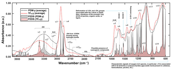
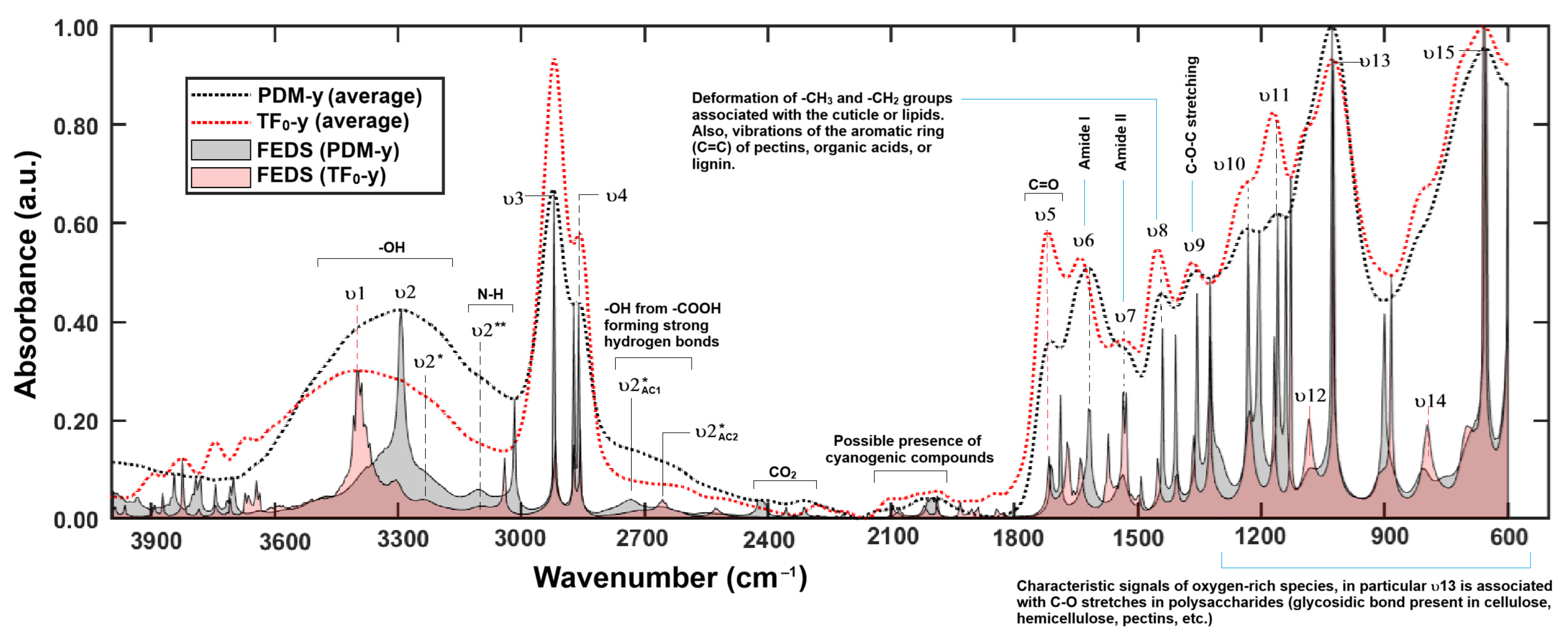
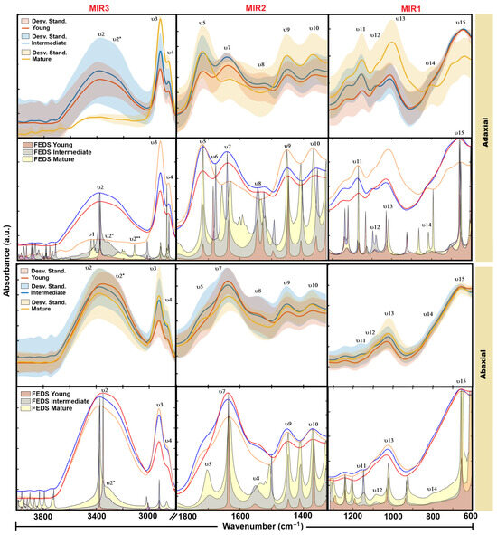
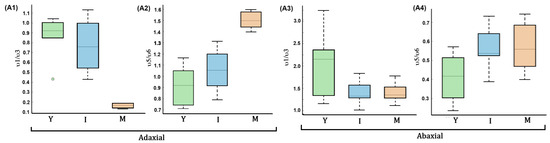
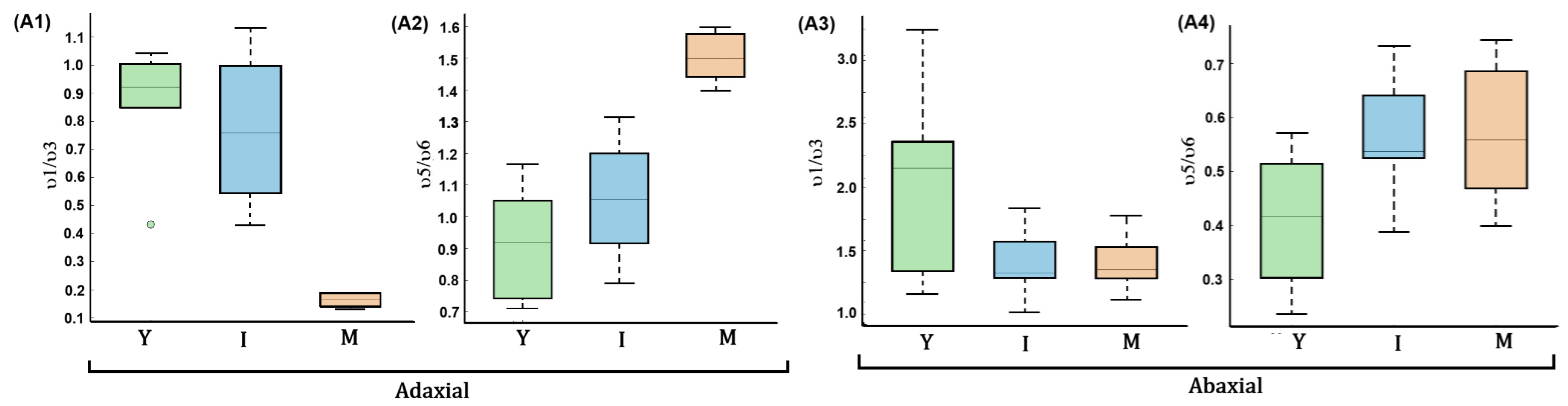
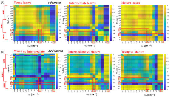
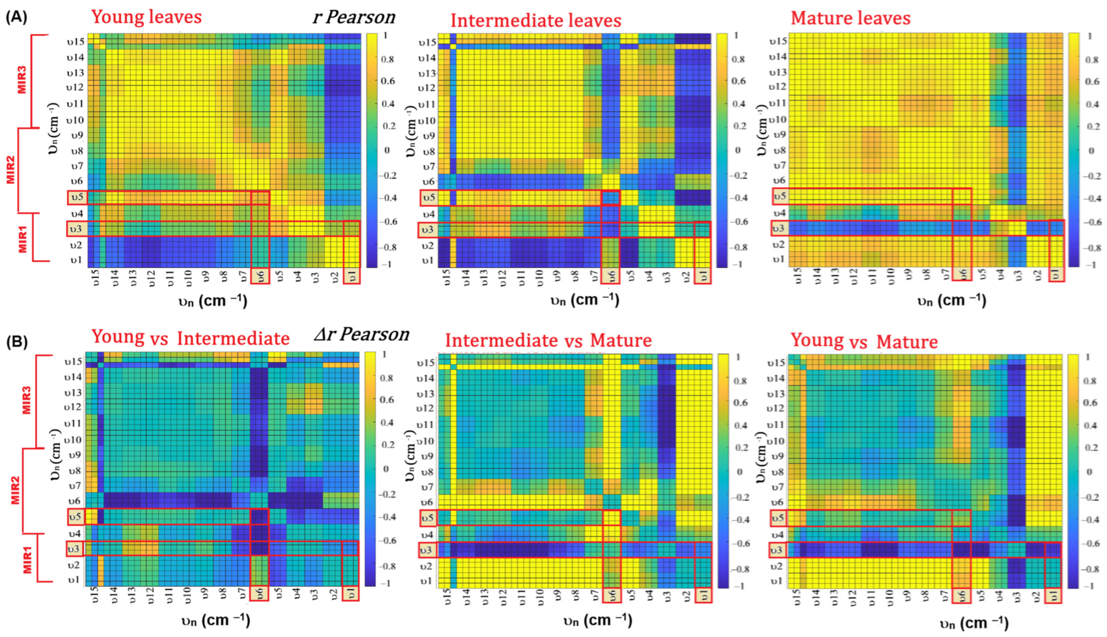
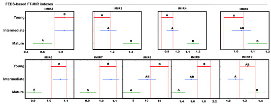
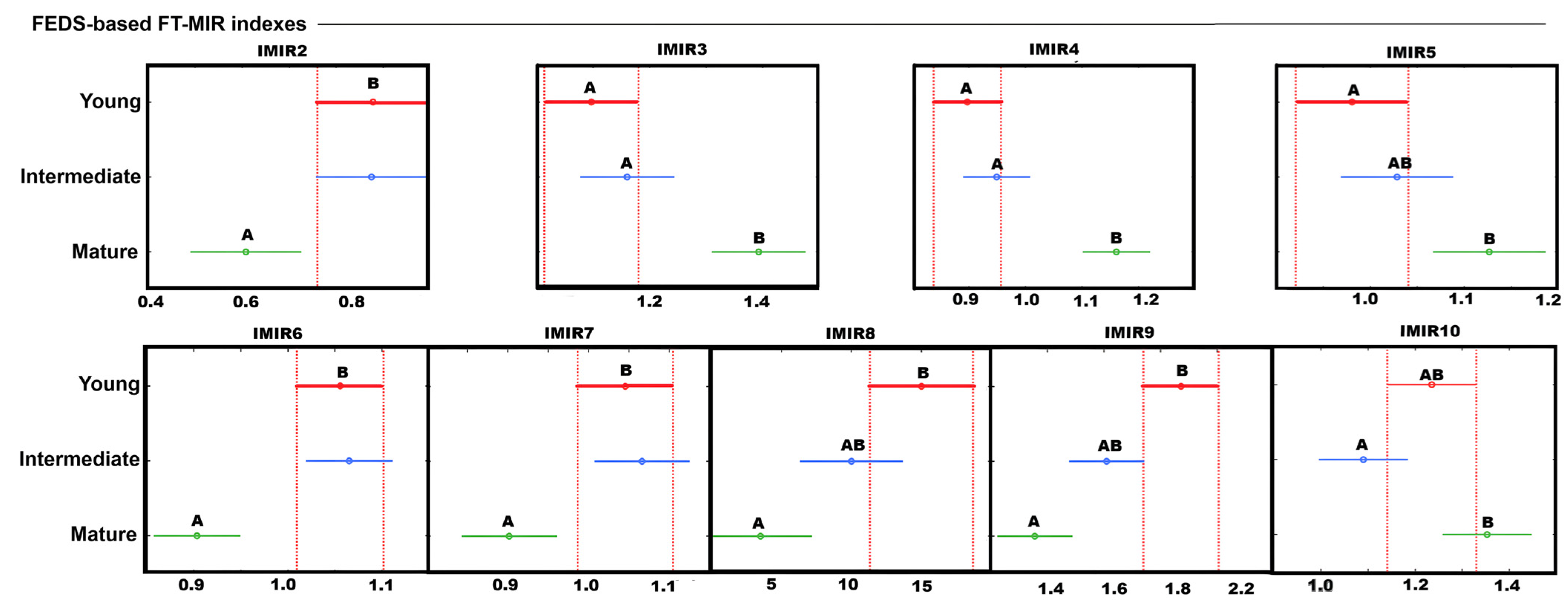
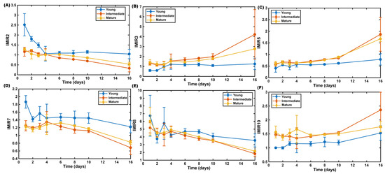
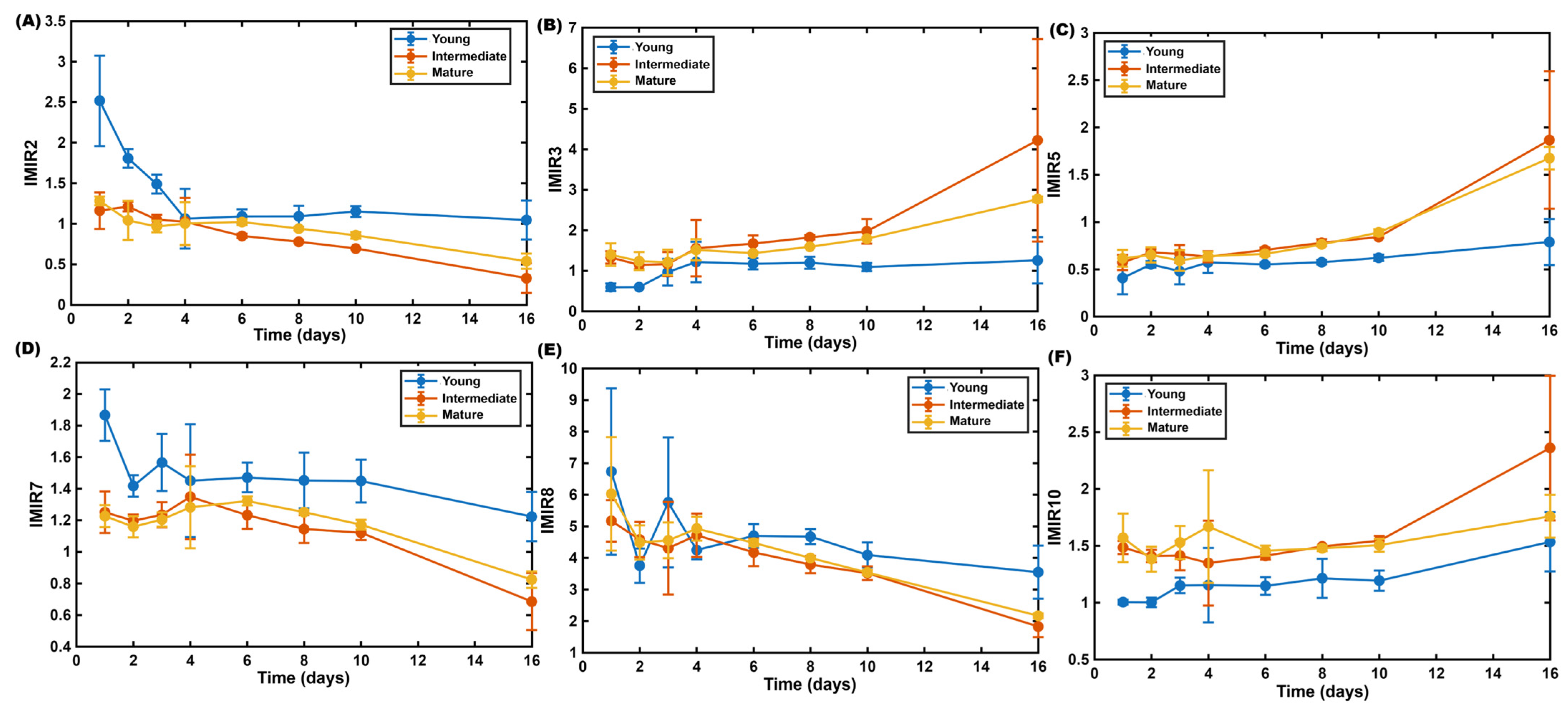
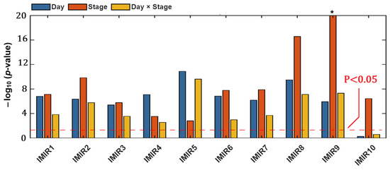
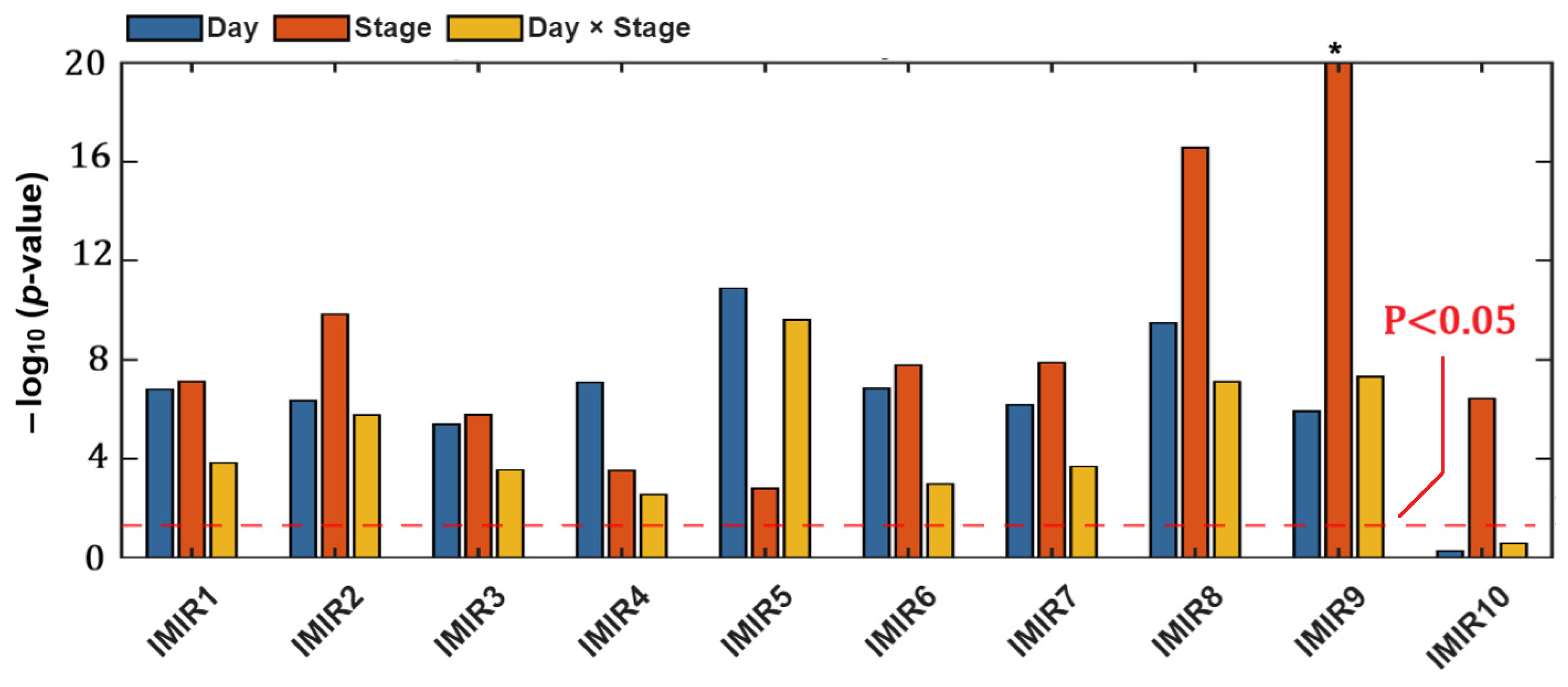
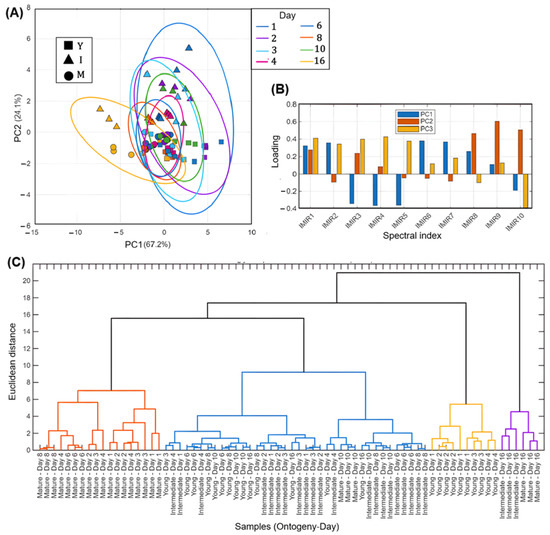
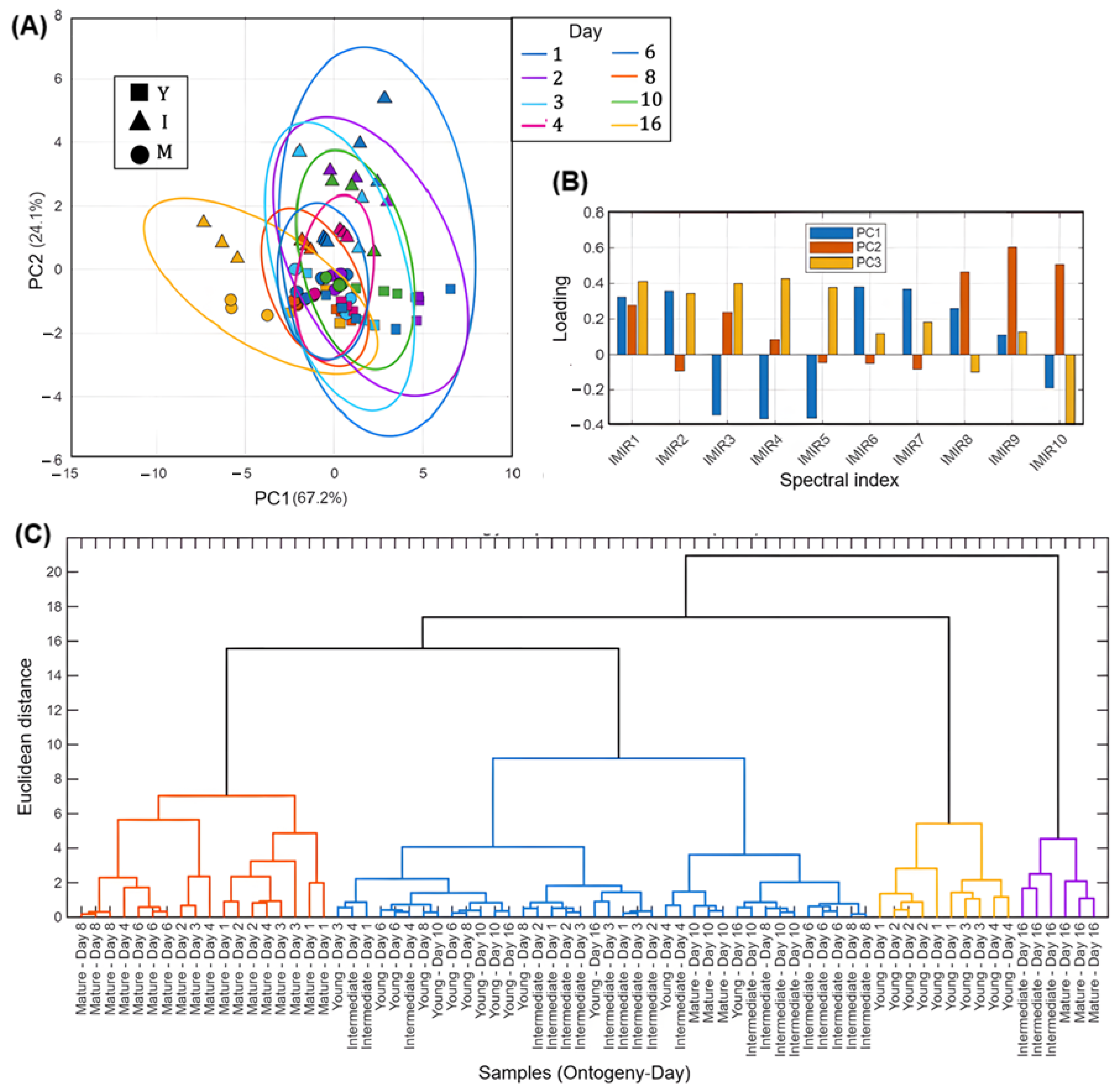
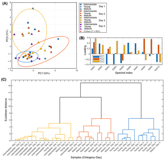
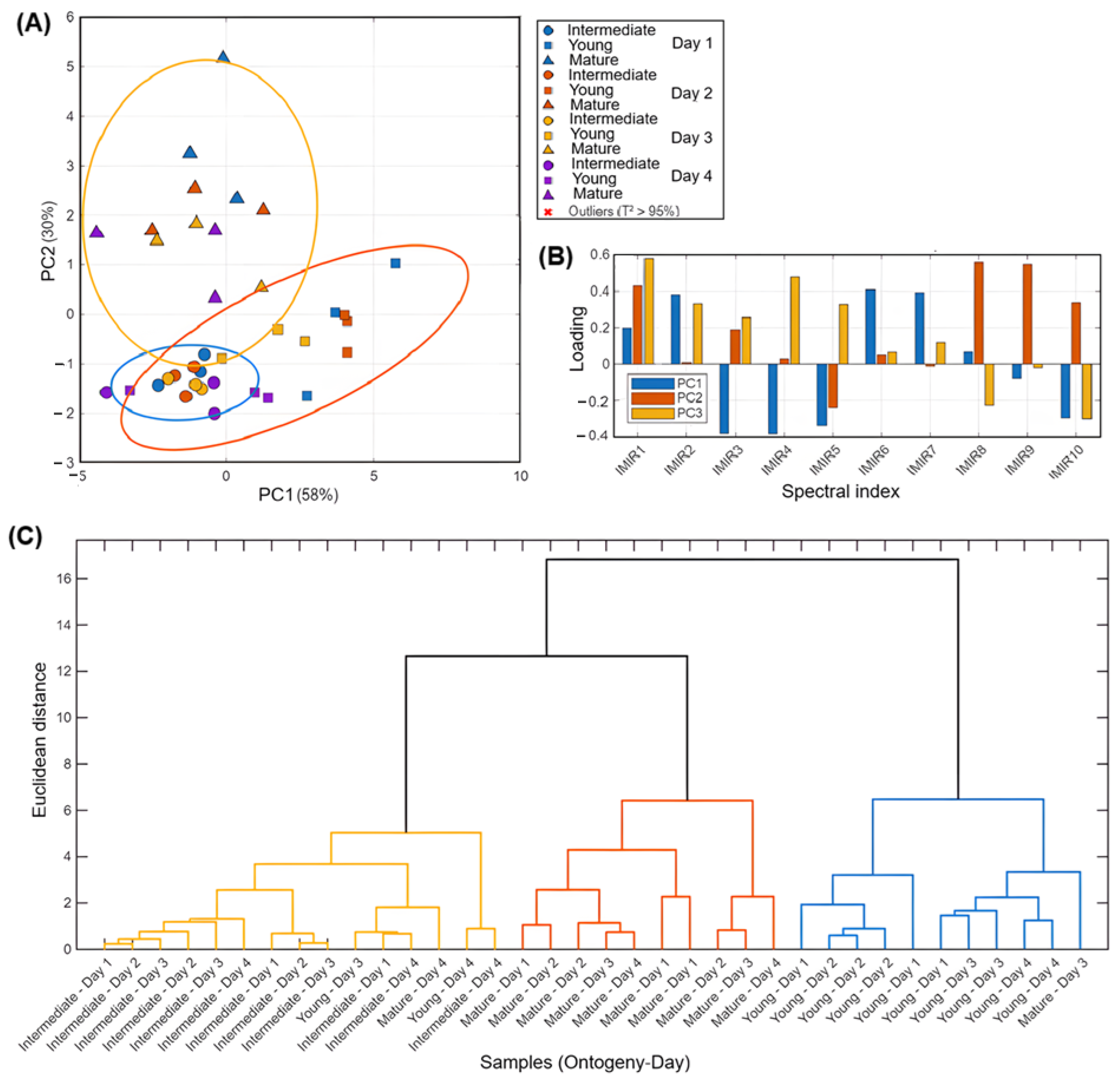

Disclaimer/Publisher’s Note: The statements, opinions and data contained in all publications are solely those of the individual author(s) and contributor(s) and not of MDPI and/or the editor(s). MDPI and/or the editor(s) disclaim responsibility for any injury to people or property resulting from any ideas, methods, instructions or products referred to in the content. |
© 2026 by the authors. Licensee MDPI, Basel, Switzerland. This article is an open access article distributed under the terms and conditions of the Creative Commons Attribution (CC BY) license.