Machine Learning for Alkali-Activated Concrete: Feature Attribution, Strength–Carbon Relationships, and the Limits of Out-of-Campaign Generalisation

Abstract

Machine learning (ML) models for alkali-activated concrete (AAC) are almost universally evaluated with random train–test splits, yet the literature-compiled datasets are strongly clustered by source study, and the reliability of such evaluations has rarely been quantified. The novelty of this study is a systematic quantification of out-of-campaign generalisation—via Leave-One-Study-Out (LOSO) cross-validation—for ML models trained on the largest curated public AAC dataset (1630 mixtures compiled from 106 published sources), together with model interpretation and an exploratory strength–carbon analysis. Four models (Linear Regression, Random Forest, Gradient Boosting, and optimised extreme gradient boosting, XGBoost) were benchmarked for predicting 28-day compressive strength (CS₂₈). XGBoost performed best under conventional random splitting, with test-set coefficient of determination R² = 0.801 and root-mean-square error (RMSE) = 7.21 MPa (5-fold cross-validation R² = 0.758 ± 0.050). Under LOSO validation across 85 study folds, however, the median R² collapsed to −0.328, with 49 of 85 folds negative: random-split metrics on literature-compiled AAC datasets are substantially inflated by within-study clustering, and study-stratified evaluation should become standard practice in this field. Within these limits, SHapley Additive exPlanations (SHAP) identified ground granulated blast-furnace slag (GGBFS) content, specimen geometry, CaO fraction, curing time, and sodium silicate (Na₂SiO₃) content as the five most influential predictors; because the oxide descriptors are derived from the declared binder proportions and the carbon-footprint values are inherited estimates from the source dataset, these attributions are associational rather than causal. No practically meaningful overall linear association was observed between estimated CO₂ footprint and CS₂₈ (Pearson r = −0.113, 95% CI [−0.175, −0.050], R² = 0.013), and a Pareto analysis identified 14 candidate low-carbon, high-strength formulations for further experimental and life-cycle assessment. The developed models are suitable for within-dataset feature attribution and exploratory screening restricted to the represented feature domain; they should not be used as external mix-design tools without validation on independent experimental campaigns.

1. Introduction

Concrete is the most widely used construction material globally, with annual production exceeding 10 billion tonnes. The production of ordinary Portland cement (OPC), its primary binder, contributes approximately 8–9% of global anthropogenic CO₂ emissions, primarily through the calcination of limestone—which alone accounts for 60% of process emissions—and the combustion of fossil fuels during clinker production at temperatures of 1400–1500° [1]. Buildings and their construction consume 36% of all energy produced worldwide and account for 39% of global CO₂ emissions [2]. In the context of escalating climate commitments and decarbonisation targets, the construction industry faces significant pressure to identify viable low-carbon alternatives. Alkali-activated concrete (AAC), synthesised from industrial by-products such as fly ash (FA), ground granulated blast furnace slag (GGBFS), and metakaolin (MK), has attracted considerable research attention due to its potential to reduce CO₂ emissions relative to OPC. Published global warming potential reductions span approximately 7–90% compared to conventional OPC-based systems; however, these figures arise from studies with different system boundaries, reference mixes, and waste-allocation assumptions and are not directly comparable [3]. Critically, activator chemistry—not precursor type—is the dominant variable controlling environmental performance, and commercial sodium silicate can largely or entirely negate the climate advantage of waste-derived precursors [4,5]. The net life-cycle CO₂ reduction compared to OPC is often only approximately 10% when alkaline activator production is fully accounted for within the system boundary, though in marine or highly corrosive service environments this figure can exceed 90% owing to the superior durability and extended service intervals of geopolymer concrete [6].

A further consideration concerns precursor supply: coal fly ash and GGBFS are in long-term decline as global decarbonisation reduces their output, and naturally abundant aluminosilicates such as calcined clays are widely viewed as the more credible route to universal deployment [7,8,9]. This outlook is directly relevant to data-driven studies such as the present one: the published literature—and therefore any dataset compiled from it, including the one used here—is dominated by FA- and GGBFS-based formulations, so the applicability of trained models to emerging precursor systems is inherently limited.

Despite its environmental promise, the commercial uptake of AAC remains limited. A primary barrier is the complexity of mix design: the mechanical performance of AAC is governed by a large number of interacting variables, including precursor chemistry, activator type and concentration, aggregate proportions, and curing conditions. Unlike OPC concrete, where well-established empirical models relate water-to-cement ratio to strength, no universally accepted design framework exists for AAC.

The need for the present research is therefore twofold. First, practitioners require screening tools that can navigate the high-dimensional AAC design space at low experimental cost; data-driven models are currently the most realistic route to such tools, but they are useful only if their reported accuracy is trustworthy. Second, the evaluation practice of the field itself requires scrutiny: almost all published ML studies on AAC report random-split metrics on the literature-compiled datasets, in which mixtures originating from the same experimental campaign can appear on both sides of the split. If these metrics are inflated by within-study clustering, the apparent maturity of ML-based AAC design is overstated and models risk being deployed far beyond their domain of validity. Quantifying the size of this inflation—and establishing a validation protocol that exposes it—is a prerequisite for credible data-driven mix design and is the central motivation of this work.

This complexity makes predictive modelling both necessary and challenging. Data-driven approaches, and machine learning (ML) in particular, have emerged as powerful tools for navigating high-dimensional design spaces in materials science [10]. Several studies have applied ML to predict AAC properties, generally reporting superior performance compared to traditional regression methods. However, these efforts have often been limited by the size and heterogeneity of their training datasets, restricting generalisability—and, importantly, most have been evaluated using random train–test splits that do not respect the boundaries between source studies, an evaluation choice whose consequences have rarely been quantified for AAC. A significant advance in data availability was recently provided by Tores et al. [11,12], who published a curated dataset of 1630 AAC formulations compiled from 106 peer-reviewed sources. This dataset, made publicly available on Zenodo (DOI: 10.5281/zenodo.7805018), represents the largest and most comprehensively curated AAC dataset in the literature, including compressive strength values at multiple ages and estimated CO₂ footprints for each formulation.

The present study exploits this resource to: (1) characterise the statistical distributions of compressive strength and CO₂ footprint across the dataset; (2) benchmark four ML models for 28-day CS prediction; (3) identify the most influential mix design variables through feature importance analysis; (4) examine the relationship between mechanical performance and environmental impact; and (5) quantify out-of-campaign generalisation through Leave-One-Study-Out cross-validation, thereby testing whether the random-split metrics conventionally reported in this field are reliable indicators of predictive transferability. The results provide feature attributions and exploratory screening tools to support rational AAC mix design, together with a methodological finding—the substantial inflation of random-split performance metrics by within-study clustering—that has direct implications for how future ML studies on literature-compiled concrete datasets should be evaluated.

2. Materials and Methods

2.1. Dataset Description

The dataset used in this study was published by Torres et al. [11,12] and is accessible at https://zenodo.org/record/7805018 (accessed on 18 May 2026). It comprises 1630 AAC formulations extracted from 106 peer-reviewed publications through systematic literature review, originally compiled by [13]. The curation process involved: elimination of redundant features, correction of transcription errors, removal of duplicate entries, and exclusion of interpolated data points. The dataset encompasses 252 variables organised into nine categories: identification features, binder oxide compositions (98 features), binder structure and content, aggregate amounts, alkali activator composition, workability, curing conditions, specimen dimensions, and mechanical/structural properties.

For this study, 28-day compressive strength (CS₂₈) was adopted as the primary target variable, as it is the standard basis for structural concrete design. Of the 969 records with valid CS₂₈ data and geometry labels, 700 used cubic specimens and 269 used cylindrical specimens; six records were removed during construction of the modelling table leaving the 963 formulations modelled here. To address the known systematic bias between specimen geometries, cylindrical values were converted to cubic-equivalent strength using the empirical conversion factor CS_cubic ≈ CS_cylindrical/0.82 (ACI 214R) [14]. Specimen geometry (is_cylindrical, binary) was additionally included as a model feature to allow the algorithms to capture any residual geometry effects not fully corrected by the conversion. The ACI 214R factor was derived primarily for ordinary Portland cement concrete; its application to alkali-activated matrices, whose brittleness and confinement behaviour vary with activator concentration and binder type, is an approximation examined further in Section 4.1 and Section 4.3. Nominal specimen dimensions are reported only heterogeneously and incompletely across the source publications and could therefore not be used as a quantitative feature; geometry is represented solely by the binary cubic/cylindrical indicator. Carbon footprint values (kg CO₂/m³), pre-calculated in the original dataset using the methodology of Alsalman et al. [4] and supplemented with oven-curing contributions, were available for 1630 formulations.

2.2. Feature Selection and Imputation

Seventeen input features were selected for modelling based on domain relevance and data completeness: binder contents (FA, GGBFS, MK, OPC in kg/m³); activator quantities (NaOH and Na₂SiO₃ in kg/m³) and NaOH molar concentration (M); total water content (kg/m³); curing temperature (°C) and initial curing duration (days); total aggregate content (kg/m³); and bulk binder oxide fractions (SiO₂, Al₂O₃, CaO, Fe₂O₃, MgO in wt%). Full details of all 17 features—including units, missingness rates, and imputation strategy—are provided in Table 1. Feature selection followed three explicit criteria rather than purely statistical screening: (i) mechanistic relevance to alkali activation as established in the AAC literature (binder quantities, activator chemistry, water, curing, aggregate); (ii) usable availability across the 106 sources, excluding variables reported too sparsely or inconsistently to be modelled (e.g., admixtures, aggregate grading, workability); and (iii) avoidance of redundancy and target leakage—of the 98 raw per-precursor oxide columns, only the five bulk oxide fractions were retained, and no feature algebraically related to CS₂₈ or CO₂ was included. No algorithmic selection (e.g., recursive feature elimination) was applied; the feature-ablation study of Section 3.9 provides a partial empirical check on the sufficiency of the retained set, and fully data-driven selection under study-stratified validation is identified as future work.

Table 1. The 17 input features used in all machine learning models, with category, unit, missingness rate in the raw dataset, and imputation strategy applied (rationale in Section 2.2).

Feature	Category	Unit	Missingness (%)	Imputation Strategy
FA	Binder	kg/m3	21.0	Zero (absent)
GGBFS	Binder	kg/m3	64.2	Zero (absent)
MK	Binder	kg/m3	96.3	Zero (absent)
OPC	Binder	kg/m3	95.2	Zero (absent)
NaOH	Activator	kg/m3	2.6	Zero
Na2SiO3	Activator	kg/m3	≤0.1	Zero
NaOH molarity	Activator	mol/L	1.1	Zero
Total water	Mix	kg/m3	≤0.1	Zero
Total aggregate	Mix	kg/m3	≤0.1	Zero
Curing temperature	Curing	°C	≤0.1	Zero
Curing time	Curing	days	32.1	Median
SiO2	Oxide	wt%	0.0	None required
Al2O3	Oxide	wt%	0.0	None required
CaO	Oxide	wt%	0.0	None required
Fe2O3	Oxide	wt%	0.0	None required
MgO	Oxide	wt%	0.0	None required
is_cylindrical	Geometry	binary	0.0	None required

Binder content features showed variable missingness: MK (96.3%), OPC (95.2%), GGBFS (64.2%), Curing_time (32.1%), FA (21.0%), NaOH_kg (2.6%), NaOH_M (1.1%), all others ≤0.1%. Missing binder, activator, water, and aggregate quantities were imputed with zero, consistent with their physical interpretation as absent components: a missing binder quantity means that precursor is absent from the formulation. Curing time was imputed with the dataset median. Oxide composition features (SiO₂, Al₂O₃, CaO, Fe₂O₃, MgO) showed zero missingness in the raw dataset—they were pre-computed weighted averages of binder oxides and were always populated, so no imputation was required. These oxide descriptors are computed in the source dataset as binder-mass-weighted averages of the oxide analyses reported for each precursor, oxide_i = Σ_β(m_β·w_iβ)/Σ_βm_β, where mᵦ is the declared quantity of binder b and w_iβ its reported mass fraction of oxide i; they are therefore deterministic functions of the declared binder proportions, not independent measurements of the actual blends (implications for redundancy and attribution are discussed in Section 3.9 and Section 4.1). Two coding ambiguities should also be noted. A NaOH molarity of zero denotes activation by sodium silicate alone, so the encoding cannot distinguish “not applicable” from a true zero concentration. Curing time refers to the initial (typically elevated-temperature) curing duration as reported by each source, which may not be defined identically across studies; the very few curing-temperature values imputed as zero (≤0.1% of records) conflate “missing” with a physical 0 °C, whereas ambient curing is recorded as the reported laboratory temperature. Specimen geometry was encoded as a binary feature (is_cylindrical: 1 = cylindrical, 0 = cubic) to allow models to capture residual geometry effects beyond the ACI 214R conversion.

2.3. Machine Learning Methodology

Four regression algorithms were implemented: Linear Regression (LR, scikit-learn v1.3) as a linear baseline; Random Forest (RF, 200 estimators); Gradient Boosting (GB, 200 estimators); and XGBoost (XGB, v2.0; [15] with hyperparameters (n_estimators = 300, max_depth = 8, learning_rate = 0.05, subsample = 0.7, colsample_bytree = 0.9, reg_α = 0.01, reg_λ = 0.5, min_child_weight = 5), selected via RandomizedSearchCV (40 iterations, inner 5-fold CV, scoring: negative RMSE) from the following search space: n_estimators ∈ {100, 200, 300, 400, 500}; max_depth ∈ {3, 4, 5, 6, 7, 8, 9, 10}; learning_rate~Uniform(0.01, 0.30); subsample~Uniform(0.50, 1.00); colsample_bytree~Uniform(0.50, 1.00); reg_α~LogUniform(10⁻³, 10); reg_λ~LogUniform(10⁻², 10); min_child_weight ∈ {1, 3, 5, 7, 10}; and gamma ∈ {0, 0.1, 0.2, 0.5}. Random Forest and Gradient Boosting were used with fixed, commonly adopted settings (200 estimators each) and were not tuned; the cross-model comparison is therefore illustrative, and the RF and GB results should be read as achievable rather than optimal performance for those algorithms. In the originally submitted analysis, imputation was applied prior to the train–test split; in this revision the entire workflow was re-implemented as a leakage-safe pipeline and all reported metrics were regenerated under it. The exact sequence is: (1) the data were split 80:20 (training n = 770, test n = 193) with a fixed seed (42); (2) all preprocessing was fitted exclusively on the training partition—zero imputation involves no estimated statistic, and the curing-time median, the only data-dependent preprocessing parameter, was estimated from training data only and re-estimated independently within the training portion of every cross-validation and LOSO fold; (3) XGBoost hyperparameters were selected by RandomizedSearchCV with the inner 5-fold search confined to the training partition; (4) the 5-fold cross-validation scores reported for model comparison were computed on the training set with the selected hyperparameters and therefore partly overlap with the model-selection folds—they should be read as within-training stability estimates rather than unbiased performance estimates, for which nested cross-validation would be required (Section 4.3); (5) the final model was refitted on the full training partition; (6) unbiased random-split performance was measured once on the untouched test set (n = 193); and (7) LOSO evaluation was run with the fold-safe preprocessing of step (2) repeated inside every study fold. Model performance was evaluated using R² and RMSE.

To quantify out-of-campaign generalisation, a Leave-One-Study-Out (LOSO) cross-validation was additionally performed for all four models: all formulations originating from one reference paper were held out at a time (86 study groups; one fold with n = 1 was excluded, as R² is undefined for a single observation, leaving 85 valid study folds). Unlike random splitting, LOSO ensures that no formulation from the held-out study is available during training, and therefore estimates the ability of the models to predict the strength of formulations from experimental campaigns entirely absent from the training data. A “study group” is defined here as one source publication (one reference in the Torres et al. [11,12] compilation); publications from the same laboratory are treated as distinct groups, so LOSO is, if anything, an optimistic proxy for cross-laboratory transfer. Of the 106 publications in the full dataset, 86 contain at least one formulation with a valid CS₂₈ value and these define the LOSO groups; the single-record group was excluded because R² is undefined for one observation, leaving 85 valid folds. XGBoost hyperparameters were fixed globally (selected once on the random-split training partition) and not retuned within LOSO folds, so LOSO evaluates a prespecified model configuration; because the tuning partition contains formulations from studies that are later held out, the LOSO estimates may even be slightly optimistic, which makes the reported generalisation gap conservative. LOSO results are summarised by the median fold-level R² and by the sample-weighted mean R², defined as the average of fold-level R² values weighted by held-out sample size. Pooled out-of-fold statistics obtained by concatenating all LOSO predictions (pooled R², RMSE, and mean absolute error, MAE), fold sample sizes, and fold-level predictions are provided with the released analysis code (Data Availability Statement), since fold-level R² can be unstable for held-out studies with few records or a narrow strength range.

Feature importance was assessed via two complementary approaches: (i) impurity-based importance (mean decrease in impurity, MDI) from RF, and (ii) SHapley Additive exPlanations (SHAP, [16,17] applied to XGB using TreeSHAP computed on the full training set—a theoretically exact algorithm that requires no subsampling. A Pareto dominance analysis identified formulations that simultaneously maximise CS₂₈ and minimise CO₂. Target leakage was explicitly verified: no predictor feature is derived from or algebraically related to CS₂₈ or CO₂ footprint. In particular, the strength efficiency metric (MPa per kg CO₂/m³ × 10³) is used solely as a visualisation variable in the strength–carbon plots (Section 3.3) and was not included in the model feature set. All analyses were performed in Python 3.12 using: scikit-learn 1.3, XGBoost 2.0, SHAP 0.43, NumPy 1.26, pandas 2.1, matplotlib 3.8, and SciPy 1.11.

2.4. Statistical Analysis

Descriptive statistics were computed for CS₂₈ and CO₂ footprint. The Pearson correlation coefficient (r) and its 95% confidence interval (Fisher z-transformation) were used to quantify the linear association between CO₂ footprint and CS₂₈. Binder type effects on CS₂₈ were visualised using box plots. The effects of NaOH molarity and curing temperature were analysed by grouping formulations into discrete bins and comparing the resulting CS₂₈ distributions.

3. Results

3.1. Dataset Characterisation

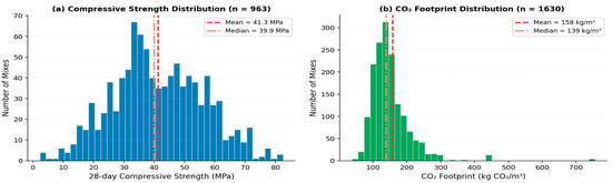
Figure 1 presents the distributions of 28-day compressive strength and CO₂ footprint across the dataset. The CS₂₈ distribution (n = 963) follows an approximately normal shape with a mean of 41.3 ± 15.0 MPa and a median of 39.9 MPa, spanning 2.3 to 82.5 MPa. This range encompasses concrete grades from structural to high-performance applications. Values in Figure 1 are as-reported; after conversion of cylindrical specimens to cubic-equivalent strength (ACI 214R, Section 2.1), the modelling dataset has a mean of 43.8 ± 16.4 MPa, a median of 42.8 MPa, and a maximum of 100.6 MPa. Unless stated otherwise, the descriptive statistics in Section 3.1, Section 3.2 and Section 3.6 refer to as-reported values, whereas all modelling, the strength–carbon correlation, and the Pareto analysis (Section 3.3, Section 3.4 and Section 3.5, and Section 3.7, Section 3.8 and Section 3.9) use cubic-equivalent values. The CO₂ footprint distribution (n = 1630) is right-skewed, with a mean of 158.0 ± 92.8 kg CO₂/m³ and a median of 139.1 kg CO₂/m³. The minimum observed footprint (38.2 kg CO₂/m³) lies well below a generic OPC literature range (280–400 kg CO₂/m³). Throughout this paper that range is shown only as an indicative literature band: it is compiled from studies whose system boundaries, functional units, transport, curing-energy treatment, and allocation assumptions are not harmonised with those underlying the present dataset, so it is not a direct benchmark, and no percentage-reduction claims are derived from it.

Figure 1. Distributions of (a) 28-day compressive strength (n = 963) and (b) CO₂ footprint (n = 1630) across the AAC dataset. Dashed lines indicate mean values; dash-dot lines indicate medians [11,12].

3.2. Influence of Precursor Binder Type

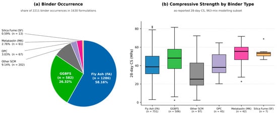
Fly ash is the most common precursor in the full dataset, present in 1286 of the 1630 formulations (78.9%), followed by GGBFS (582; 35.7%); expressed as shares of all binder occurrences, FA and GGBFS account for 58.2% and 26.3% respectively (Figure 2a). Within the 963-mix modelling subset, FA appears in 751 mixes (78.0%) and GGBFS in 506 (52.5%), and these counts are indicated in Figure 2b. Metakaolin, silica fume, and OPC appear in fewer than 5% of mixes each, reflecting the predominance of FA and GGBFS in AAC research. A further 202 formulations (12.4%) contain other supplementary cementitious materials, which together account for 9.1% of all binder occurrences (Figure 2a). Compressive strength distributions by binder type (a mix containing two precursors appears in both groups) reveal important differences (Figure 2b). Formulations based on GGBFS exhibit the highest median CS₂₈ among FA- and GGBFS-containing mixes, consistent with the higher CaO content and reactivity of slag. Metakaolin-based formulations also show competitive strength values, albeit with greater variability, attributed to their high amorphous content and sensitivity to Si/Al ratios. Mixes containing other supplementary cementitious materials show the lowest median 28-day strength of any group (25.3 MPa; n = 97).

Figure 2. (a) Share of binder occurrences across the full dataset (n = 1630 formulations, 2211 binder occurrences; a mix containing two precursors contributes two occurrences). (b) Box plots of 28-day compressive strength (as-reported) stratified by binder type within the 963-mix modelling subset; whiskers extend to 1.5× IQR.

3.3. CO₂ Footprint vs. Compressive Strength

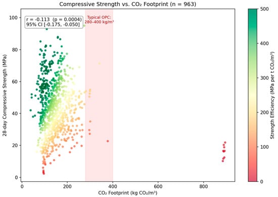
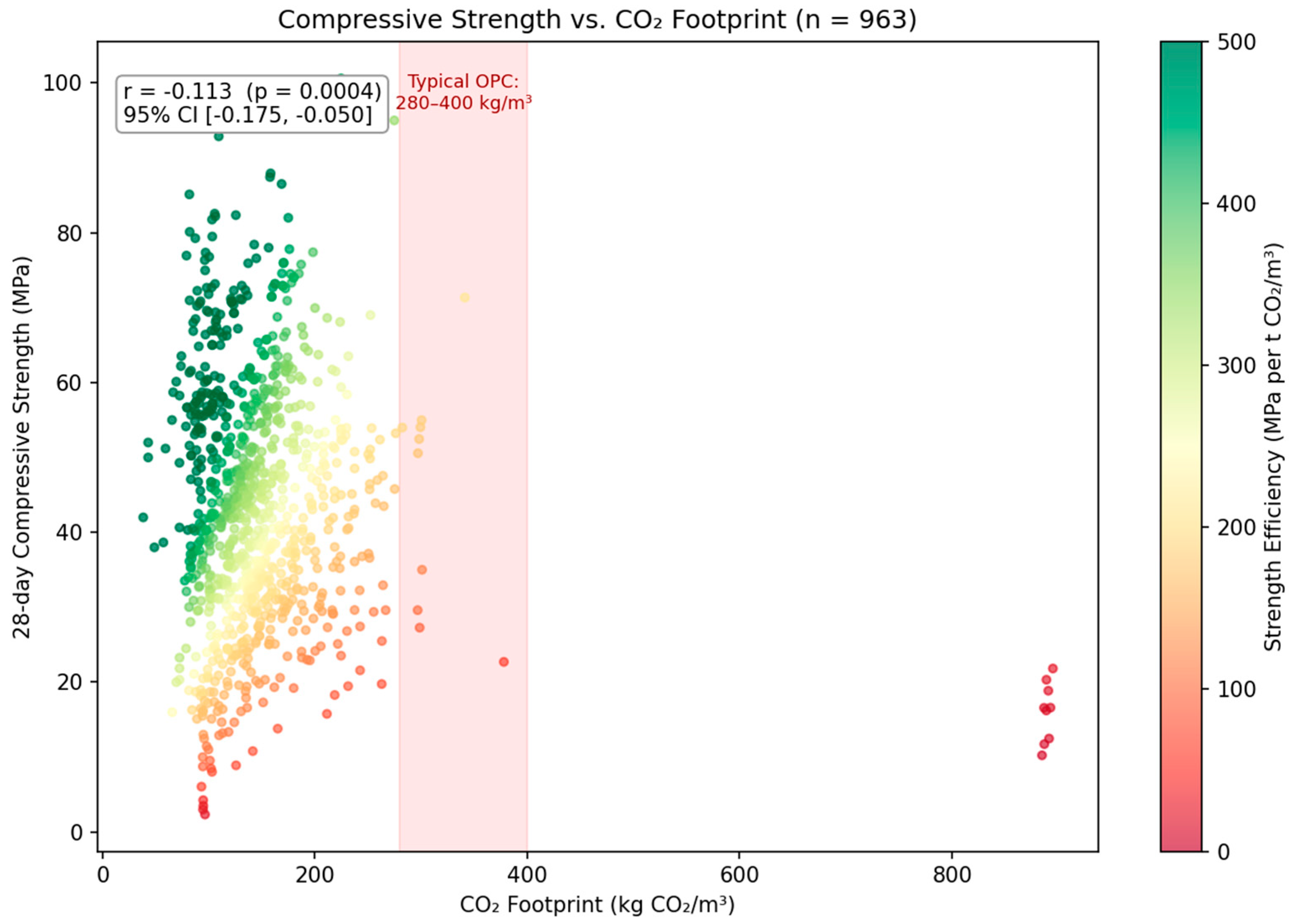
Figure 3 plots CS₂₈ against CO₂ footprint for the 963 formulations with both measurements. The Pearson correlation coefficient is r = −0.113 (p = 0.0004, 95% CI [−0.175, −0.050]), indicating a statistically significant but practically negligible weak negative association. This result warrants careful interpretation: with n = 963, statistical power is very high, so even trivially small correlations may reach significance; the effect size (r = −0.113, R² = 0.013) explains less than 1.3% of the variance in CS₂₈ and is thus negligible from a practical standpoint. Formulations achieve CS₂₈ values above 60 MPa at footprints below 150 kg CO₂/m³, showing that the weak negative trend does not preclude high-performance, low-carbon formulations. Multi-objective mix optimisation that minimises CO₂ without sacrificing mechanical performance is supported by these data. The bivariate correlation is, however, potentially confounded by binder type, activator system composition, and curing regime; this confounding, and the partial correlation analysis needed to address it, are examined in Section 4.2.

Figure 3. Compressive strength versus CO₂ footprint for 963 AAC formulations. Colour represents strength efficiency (MPa per kg CO₂/m³ × 10³). The shaded band indicates an indicative literature range for OPC concrete (280–400 kg/m³); system boundaries and allocation assumptions are not harmonised with the present dataset, so the band is not a direct benchmark (Section 3.1). Pearson r = −0.113 (p = 0.0004); effect size R² = 0.013 is negligible.

3.4. Model Performance Under Random Splitting

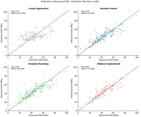
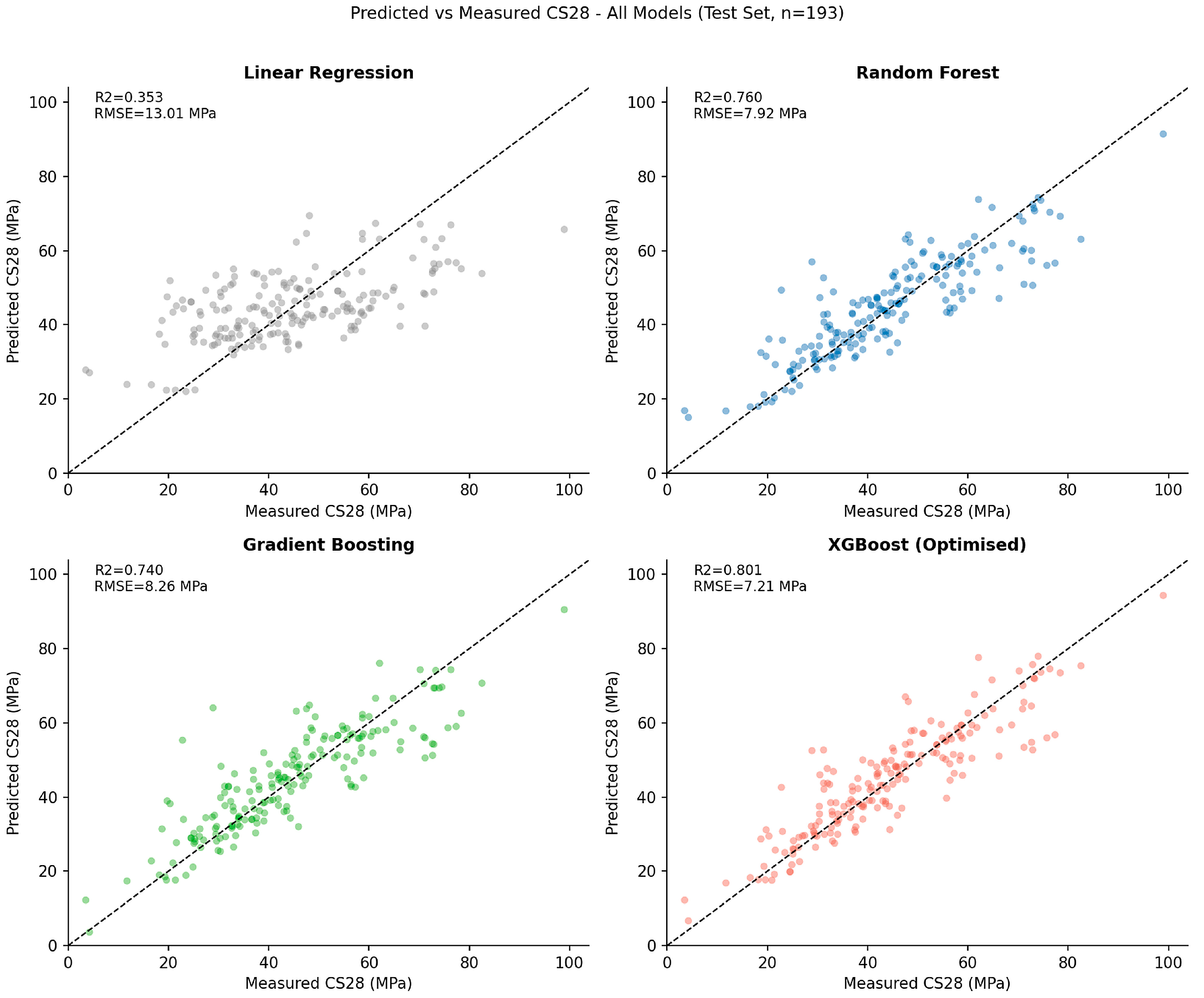
Table 2 summarises performance metrics for all four models. XGBoost achieved the best test-set performance under random splitting (R² = 0.801, RMSE = 7.21 MPa), ahead of RF (R² = 0.760), GB (R² = 0.740), and LR (R² = 0.353). Bootstrap 95% CIs for test-set R² (1000 resamples) were: LR [0.237–0.453], RF [0.682–0.825], GB [0.637–0.810], and XGB [0.734–0.858]. All four models were evaluated with 5-fold CV for a fair comparison: XGB (CV R² = 0.758 ± 0.050), RF (0.710 ± 0.059), GB (0.706 ± 0.059), and LR (0.205 ± 0.097). The gap between LR test-set and CV R² reflects the known instability of linear regression in high-dimensional, multi-collinear feature spaces when evaluated on heterogeneous multi-source datasets. The ensemble models show more consistent test–CV alignment. A paired Wilcoxon signed-rank test on the 5-fold CV scores (RF vs XGB) yields p = 0.0625; with only five paired observations this test has minimal statistical power and is reported for completeness only. The absence of statistical significance must not be read as evidence that the two models perform equivalently—the overlapping bootstrap 95% CIs simply indicate that these data do not resolve the difference.

Table 2. Model performance on the held-out test set (n = 193) and 5-fold cross-validation on the training set (n = 770). RMSE in MPa. Out-of-campaign (LOSO) results are reported separately in Section 3.5.

Model	R2 (Test)	RMSE (MPa)	CV R2 (±std)
Random Forest	0.760	7.92	0.710 ± 0.059
Gradient Boosting	0.740	8.26	0.706 ± 0.059
Linear Regression	0.353	13.01	0.205 ± 0.097
XGBoost (Optimised)	0.801	7.21	0.758 ± 0.050

Figure 4 presents predicted vs measured CS₂₈ for all four models on the held-out test set (n = 193). XGBoost produces the tightest scatter around the 1:1 line (R² = 0.801), followed by RF (R² = 0.760), GB (R² = 0.740), and LR (R² = 0.353). All ensemble models slightly underpredict above 60 MPa, consistent with the lower density of high-strength mixes in the training data. As shown in the following section, these random-split figures represent an optimistic upper bound on predictive performance.

Figure 4. Predicted vs. measured CS₂₈ for all four models on the test set (n = 193). Dashed line = 1:1. Specimen geometry correction (ACI 214R, ÷0.82) applied to cylindrical values prior to modelling.

3.5. Out-of-Campaign Generalisation: Leave-One-Study-Out Cross-Validation

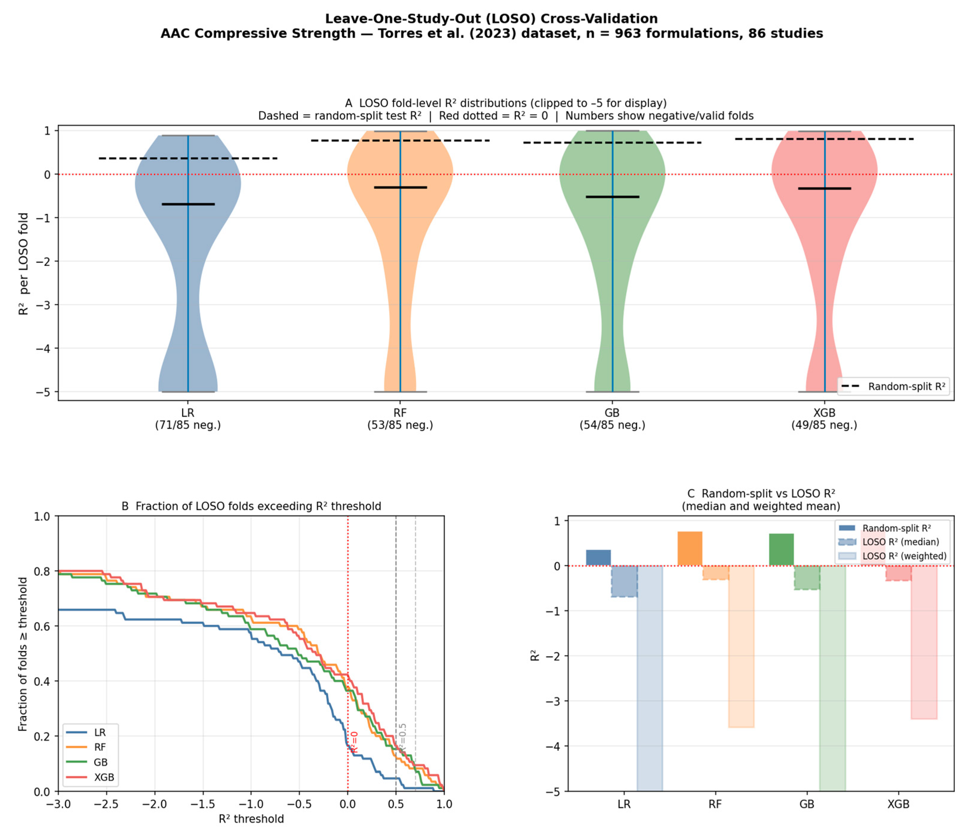
LOSO cross-validation (Section 2.3) reveals that out-of-campaign generalisation is substantially weaker than the random-split metrics suggest (Figure 5). The median LOSO R² values are: XGBoost −0.328, RF −0.304, GB −0.523, and LR −0.691. The fraction of folds with negative R² is 49/85 (58%) for XGBoost, 53/85 (62%) for RF, 54/85 (64%) for GB, and 71/85 (84%) for LR. Only 14/85 XGBoost folds achieve R² ≥ 0.5. Fold-level R² should be interpreted with care: it can become strongly negative when a held-out study contains few observations or a narrow strength range. For this reason, the median and the sample-weighted mean R² (Section 2.3) are reported together in Figure 5, and the pooled out-of-fold error statistics (pooled R², RMSE, MAE) and fold sample sizes are released with the analysis code. The qualitative conclusion—that within-campaign interpolation does not transfer to unseen campaigns—is robust to the choice of summary statistic.

Figure 5. Leave-One-Study-Out (LOSO) cross-validation across 85 valid study folds. (A) Fold-level R² distributions per model (clipped to −5 for display); dashed lines = random-split test R²; horizontal bars = LOSO medians. (B) Fraction of folds exceeding a given R² threshold. (C) Random-split R² versus LOSO median and sample-weighted mean R², illustrating the gap between within-campaign interpolation and out-of-campaign generalisation [11,12].

The random-split R² = 0.801 should therefore be interpreted strictly as an optimistic upper bound under within-campaign interpolation; it does not reflect the model’s ability to predict the strength of formulations from experimental campaigns absent from the training data. The mechanisms underlying this gap, and its implications for evaluation practice in the field, are discussed in Section 4.1.

3.6. Associations of Process Parameters with Strength

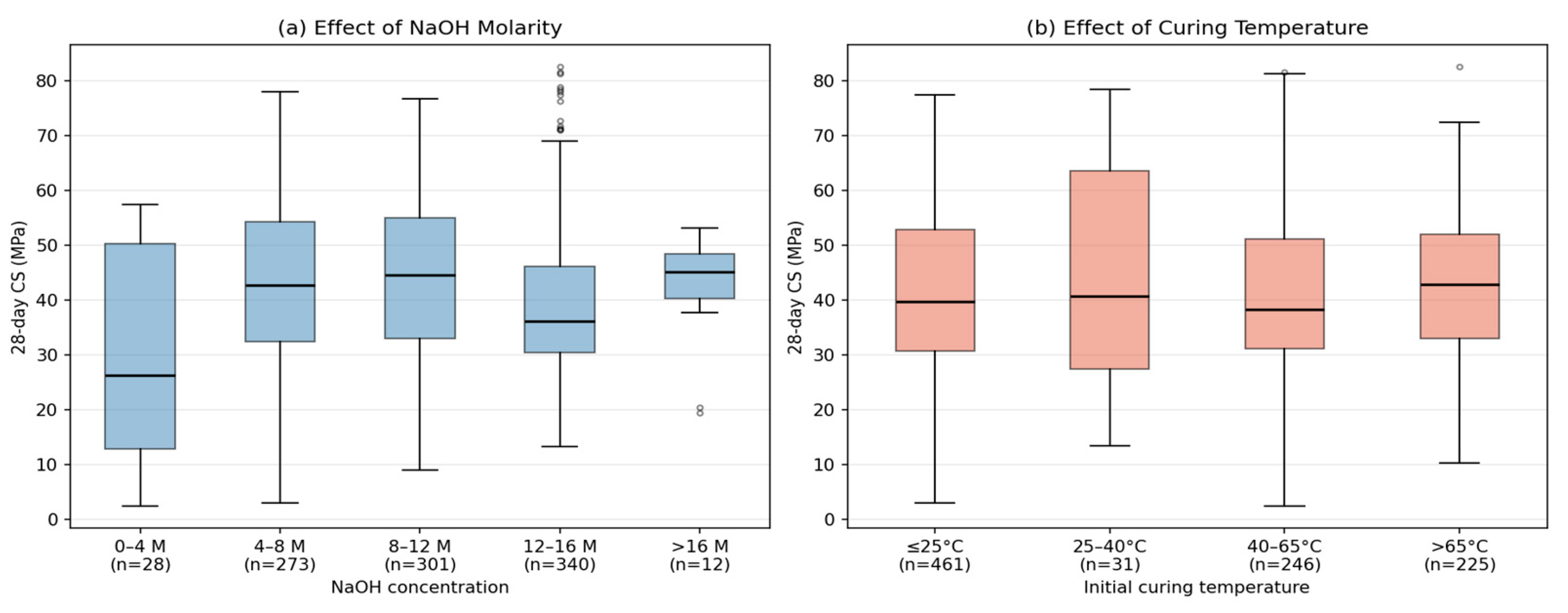
Figure 6 examines the association of two key process variables with CS₂₈. NaOH molarity (Figure 6a) shows a non-monotonic relationship: median CS₂₈ rises from 26.2 MPa at very low concentrations (0–4 M; n = 28) to a peak of 44.5 MPa at 8–12 M (n = 301), then falls to 36.1 MPa at 12–16 M (n = 340). This pattern is consistent with the literature, where insufficient alkalinity limits precursor dissolution while excessive hydroxide concentration can interfere with gel formation and reduce strength. The small group at >16 M (n = 12) yields a high median (45.1 MPa) but lacks sufficient representation for robust conclusions.

Figure 6. Association of (a) NaOH molar concentration and (b) curing temperature with 28-day compressive strength. Box plots show median, interquartile range, and 1.5× IQR whiskers. Sample sizes (n) are indicated for each group.

Curing temperature (Figure 6b) shows only modest differences between groups: median CS₂₈ is 39.7 MPa for ambient curing (≤25 °C; n = 461), 40.7 MPa at 25–40 °C (n = 31), 38.2 MPa at 40–65 °C (n = 246), and 42.8 MPa for heat curing above 65 °C (n = 225). The slightly higher median under high-temperature curing is consistent with the thermal-activation requirements of low-calcium, FA-rich systems, but the differences between groups are small relative to the within-group spread and should be interpreted cautiously: curing regimes are strongly confounded with binder type and alkali-activator dose across the source studies. Stratified analysis by precursor family would be required before drawing mechanistic conclusions, and the small sample at 25–40 °C (n = 31) limits inference for that range.

3.7. Feature Importances: Impurity-Based (MDI), SHAP, and Gain-Based Attribution

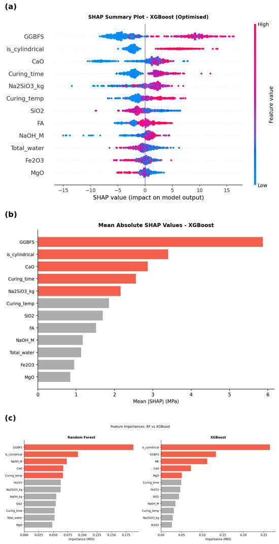
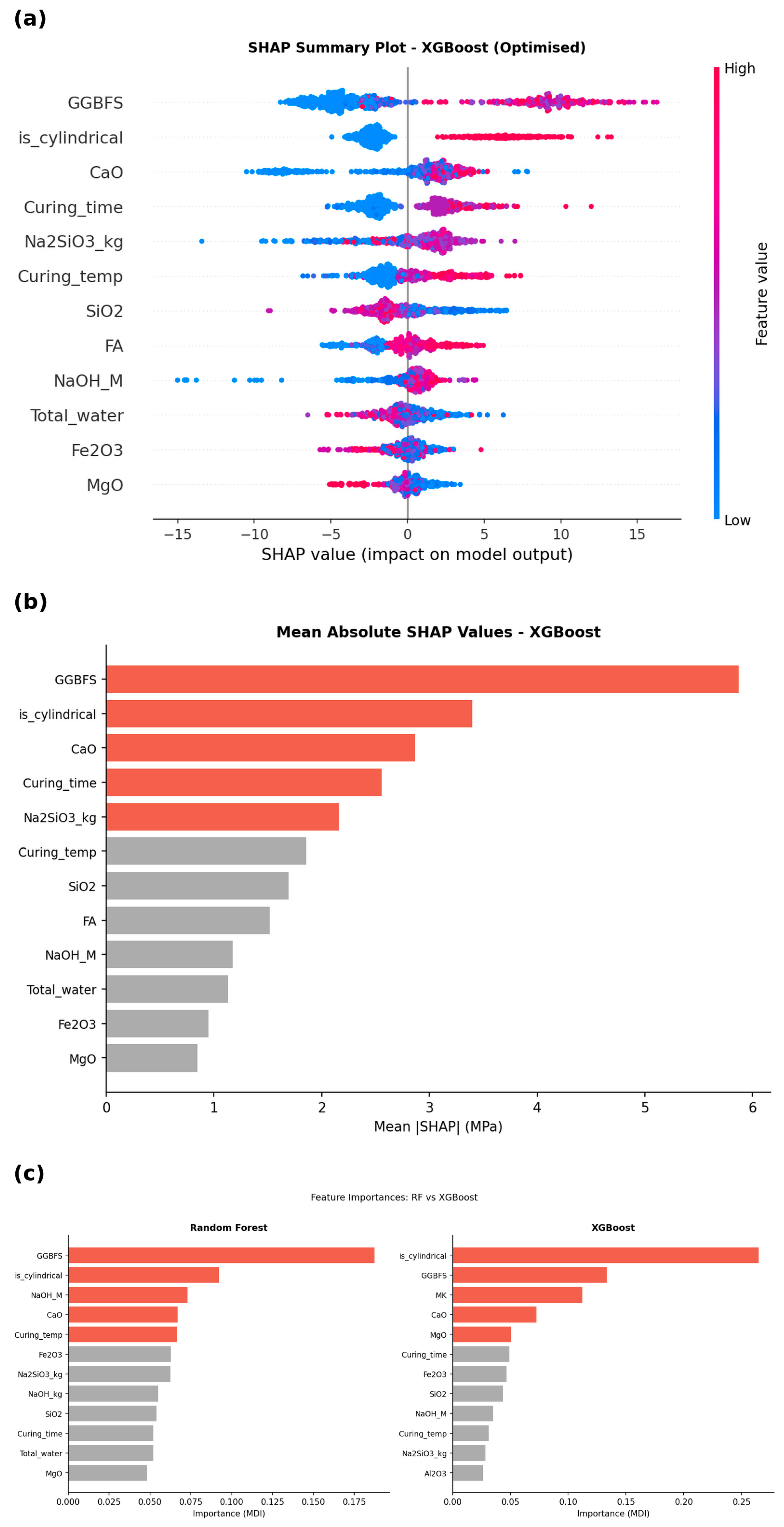
Figure 7 presents the feature attribution analyses: the SHAP beeswarm plot (Figure 7a) and mean absolute SHAP values (Figure 7b) for the optimised XGBoost model—computed via TreeSHAP on all 770 training samples, an exact algorithm requiring no subsampling—together with the native impurity/gain-based (MDI) importances for RF and XGBoost (Figure 7c).

Figure 7. Feature attribution for the trained models. (a) SHAP beeswarm plot for the optimised XGBoost model (all n = 770 training samples, TreeSHAP exact); each point = one sample; horizontal position = SHAP value (MPa); colour = feature value (red = high, blue = low). (b) Mean absolute SHAP values (XGBoost); red bars = top five predictors. (c) Native impurity/gain-based (MDI) feature importances for Random Forest and XGBoost; red bars = top five predictors per model. XGBoost MDI ranks specimen geometry first, whereas SHAP ranks GGBFS first, illustrating the sensitivity of importance rankings to the attribution method.

GGBFS content yields the largest mean absolute SHAP value, with high GGBFS values consistently producing large positive SHAP contributions, a pattern consistent with the calcium-rich binder’s dual role in supplying reactive calcium for C-S-H and C-A-S-H gel formation and modifying the Si/Al ratio. Specimen geometry (is_cylindrical) ranks second. This should not be read primarily as a material-behaviour finding: beyond any residual physical geometry effect not removed by the ACI 214R conversion, the geometry indicator is strongly associated with source study—most studies use a single specimen shape—and may therefore act partly as a proxy for study identity, national testing standard, and laboratory practice (Section 4.1). CaO fraction shows a positive SHAP profile, consistent with supplementary calcium provision. Curing time exerts a monotonically positive SHAP effect, consistent with the kinetic benefit of extended curing for geopolymerisation. Na₂SiO₃ quantity shows predominantly positive SHAP values at moderate doses, reflecting the silicate activator’s role in Si/Al ratio control.

The attribution methods agree on the dominant predictor but diverge thereafter. RF impurity-based (MDI) importance and XGBoost SHAP attribution both rank GGBFS first, whereas XGBoost’s native gain-based (MDI) importance ranks specimen geometry first (Figure 7c). NaOH_M appears third in the RF MDI ranking but lower in SHAP, suggesting that its MDI importance is partly inflated by high cardinality (continuous variable with many splits) rather than genuine predictive contribution. SHAP, being grounded in cooperative game theory, avoids this cardinality bias, but it is not immune to feature dependence, confounding, or dataset bias: with strongly correlated predictors (e.g., GGBFS content and CaO fraction, the latter derived from binder proportions; curing conditions that differ systematically between binder families; and related activator quantity and molarity), attributions may be divided among correlated representations. All rankings reported here therefore describe associations learned by the model within this dataset, not causal material mechanisms; assessing ranking stability across resampling and LOSO folds, and complementing SHAP with permutation importance and grouped (chemically related) features, is identified as required follow-up in Section 4.3.

3.8. Pareto Efficiency Frontier

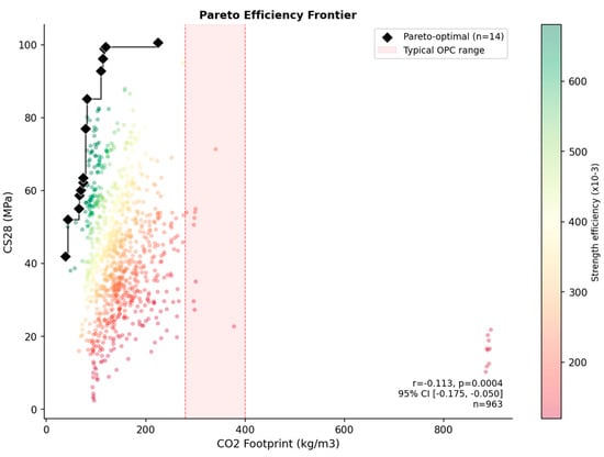
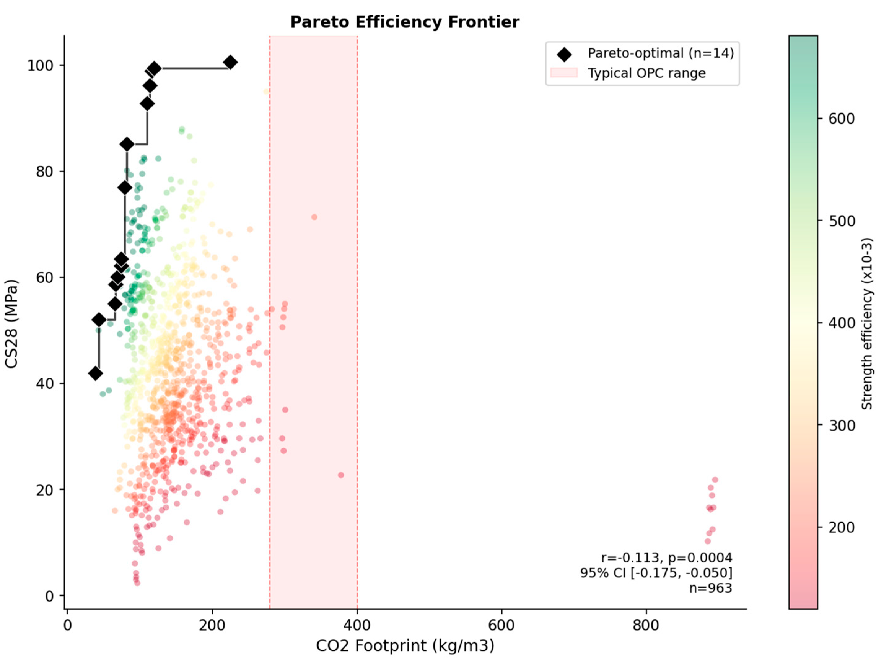
Figure 8 presents the Pareto efficiency frontier for the 963 formulations with both CS₂₈ and CO₂ footprint data. The Pareto front (n = 14 formulations, black diamonds) represents mixes for which no other formulation achieves equal or better performance on both objectives simultaneously. These Pareto-optimal mixes span 38–225 kg CO₂/m³ and 42–101 MPa (cubic-equivalent), with thirteen of the fourteen achieving structural-grade strength (≥40 MPa) at CO₂ footprints below 120 kg CO₂/m³—well below the OPC reference band (280–400 kg/m³). The weak bivariate correlation reported in Section 3.3 shows that, across this heterogeneous dataset, no practically meaningful overall linear association exists between the two objectives; multi-objective mix design that minimises CO₂ without sacrificing strength is therefore not precluded. The Pareto frontier identifies the specific formulations that best exploit this observation. Table 3 reports the key compositional and performance attributes of all 14 Pareto-optimal formulations (binder type, GGBFS and FA content, Na₂SiO₃ and NaOH dosages, curing temperature and duration, CS₂₈, and CO₂ footprint), providing candidate formulations for further experimental and life-cycle assessment. The frontier is dominated by FA/GGBFS blends and GGBFS-rich mixes activated predominantly with sodium silicate at moderate dosages and cured at ambient to moderately elevated temperatures (24–60 °C); the single highest-strength mix requires both a high activator dose and 80 °C curing, and carries a correspondingly higher footprint. Frontier membership is itself uncertain: the CO₂ values are inherited estimates that exclude or simplify transport, regional energy mix, the sodium-silicate production pathway, and by-product allocation, and the strength values depend on the assumed cylinder-to-cube conversion, so a modest change in an emission factor or conversion factor can move individual mixtures on or off the deterministic frontier. The 14 formulations should accordingly be read as screening candidates whose frontier status must be confirmed by a sensitivity analysis over emission-factor and conversion-factor assumptions—identified in Section 4.3 as a necessary step before any experimental adoption.

Figure 8. Pareto efficiency frontier: CS₂₈ vs CO₂ footprint (cubic-equivalent; n = 963 formulations). Black diamonds = Pareto-optimal mixes (Table 3; n = 14). Colour = strength efficiency. Shaded band = indicative OPC literature range, not a direct benchmark (Section 3.1). Pearson r and 95% CI shown.

Table 3. Compositional and performance attributes of the 14 Pareto-optimal formulations (sorted by ascending CO₂ footprint). Reference numbers follow the source-study identifiers of the Torres et al. [11,12] dataset. CS₂₈ values are cubic-equivalent (ACI 214R, ÷0.82); CO₂ footprints follow the methodology of Alsalman et al. [4]. MK and OPC contents are zero for all 14 mixes. A NaOH dosage of 0 kg/m³ denotes activation by sodium silicate solution alone.

Binder System	FA (kg/m3)	GGBFS (kg/m3)	NaOH (kg/m3)	NaOH (M)	Na2SiO3 (kg/m3)	Curing T (°C)	Curing Time (d)	CS28 (MPa)	CO2 (kg/m3)
FA/GGBFS	291	97	25	3	50	25	1	42	38.2
FA/GGBFS	194	194	25	3	50	25	1	52	42.9
FA/GGBFS	194	194	25	3	50	60	1	55	65.3
GGBFS	0	424	16	12.5	58	25	1	58.7	66.4
FA/GGBFS	200	200	0	0	74	24	1	60.1	69.4
GGBFS	0	424	20	12.5	70	25	1	62.2	73.7
FA/GGBFS	100	300	0	0	74	24	1	63.5	74.2
GGBFS	0	400	0	0	74	24	1	77	79
FA	381	0	49	8	122	25	0.75	85.1	81.7
FA/GGBFS	200	200	0	12.7	129	60	1	92.9	109.4
FA/GGBFS	120	280	0	12.7	129	60	1	96.2	113.2
FA/GGBFS	60	340	0	12.7	129	60	1	99	116.1
GGBFS	0	400	0	12.7	129	60	1	99.4	119
FA	416	0	65	15	292	80	1	100.6	224.6

3.9. Feature Ablation Study

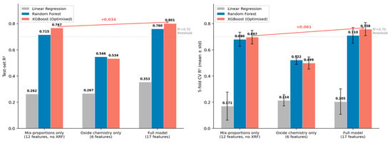
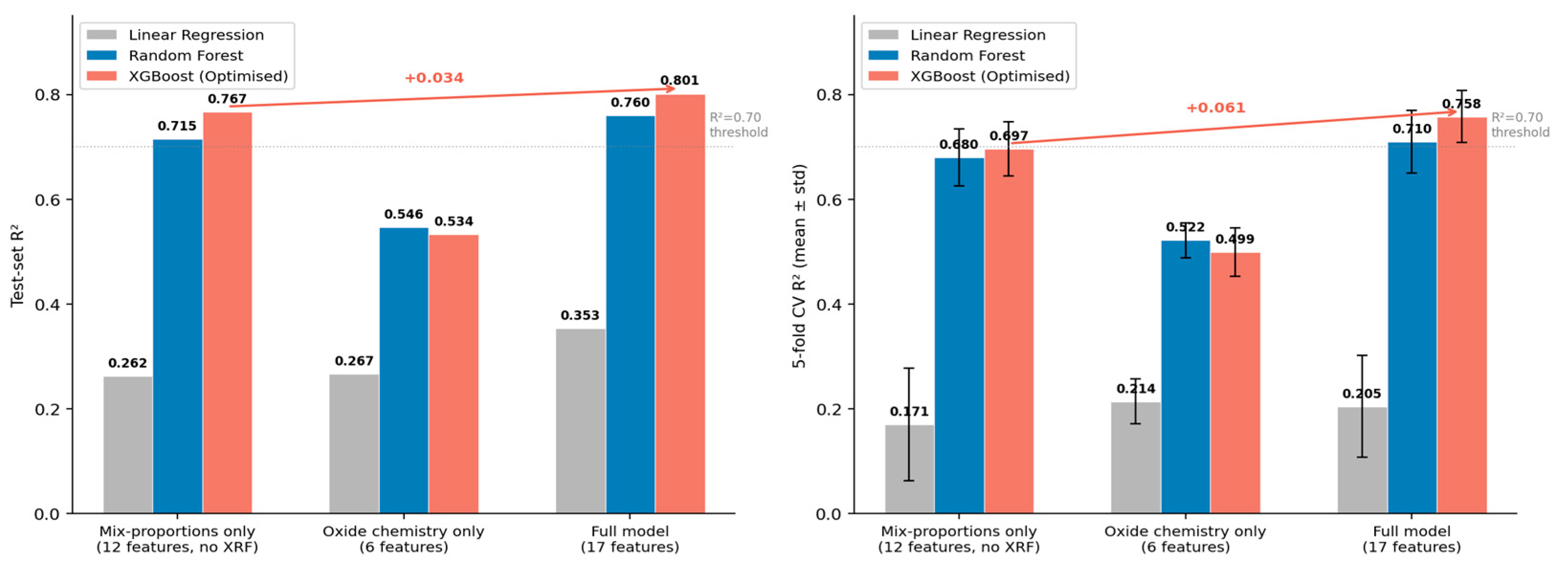
To assess the relative contribution of mix-proportioning information vs oxide chemistry to predictive performance, three XGBoost models were trained on mutually exclusive feature subsets: (i) mix-proportions only (12 features: binder quantities, activator, water, curing, and specimen geometry)—the information available without XRF analysis; (ii) oxide chemistry only (six features: SiO₂, Al₂O₃, CaO, Fe₂O₃, MgO, and specimen geometry); and (iii) full model (17 features). Results are presented in Table 4 and Figure 9.

Table 4. Feature ablation results (XGBoost, RF, LR) across three feature subsets. ΔR² = reduction vs full model (XGBoost).

Feature Subset	LR R2	RF R2	XGB R2	ΔR2 (XGB)
Mix proportions only (12 features)	0.262	0.715	0.767	−0.034
Oxide chemistry only (six features)	0.267	0.546	0.534	−0.268
Full model (17 features)	0.353	0.760	0.801	—

Figure 9. Feature ablation study: test-set R² (left) and 5-fold CV R² ± SD (right) for LR, RF, and XGBoost across three feature subsets. Dotted line = R² = 0.70 reference.

The mix-proportions-only XGBoost achieves R² = 0.767 (RMSE = 7.81 MPa, CV R² = 0.697 ± 0.052), i.e., a direct reduction in ΔR² = 0.034 and an RMSE increase of 0.60 MPa relative to the full model under random splitting. A practitioner without XRF data therefore loses little random-split accuracy using only routine mix-design information. Three caveats apply. First, a ratio of R² values is not a rigorous measure of retained predictive information, so only the direct metric differences are reported. Second, the oxide-chemistry features (SiO₂, Al₂O₃, CaO, Fe₂O₃, and MgO) are weighted averages derived from the declared binder proportions rather than independent measurements (Section 2.2): the mix-proportions subset already implicitly encodes precursor oxide chemistry through the binder dosages, so this ablation quantifies the redundancy of the pre-calculated oxide descriptors rather than any independence of chemical reactivity from mix proportioning. Third, because random-split metrics overstate transferability (Section 3.5), practical conclusions about which feature set is sufficient should ultimately rest on study-stratified evaluation; repeating the ablation under LOSO or grouped cross-validation is identified as required follow-up and is directly supported by the released code. In contrast, the oxide-chemistry-only model performs substantially worse (R² = 0.534, RMSE = 11.05 MPa), confirming that oxide ratios alone are insufficient without knowing the physical quantities and curing protocol.

Two implications follow. First, the marginal gain of including oxide chemistry (+0.034 R² points) must be weighed against the data-collection burden: XRF analysis is not routinely available on-site, and oxide compositions are frequently missing in the literature (MK rows: 96.3% missing; OPC rows: 95.2%). Second, the oxide-only model’s poor performance (R² = 0.534) demonstrates that geochemistry alone does not govern CS₂₈: quantity and curing matter at least as much as precursor composition.

4. Discussion

4.1. Predictive Modelling and the Generalisation Gap

The central methodological finding of this study is the gap between random-split and study-stratified evaluation. The optimised XGBoost model achieved R² = 0.801 on the held-out test set and a 5-fold CV R² of 0.758 ± 0.050 (Section 3.4), yet its median LOSO R² was −0.328 with 58% of study folds negative (Section 3.5). This gap arises because random folds do not respect study boundaries: formulations from the same research group share procedural protocols (mixing sequence, aggregate source, storage) that are not encoded in numeric features, creating within-cluster homogeneity that the models exploit as study-specific fingerprints. This is a well-documented limitation of multi-source concrete ML datasets (Li et al. [10]). The practical consequence is that the models developed here are appropriately characterised as tools for within-dataset feature attribution and data exploration, not for external mix design. More broadly, study-stratified cross-validation should be adopted as the standard evaluation protocol in future ML studies using the literature-compiled AAC datasets; random-split metrics reported without a study-stratified counterpart risk substantially overstating predictive transferability. The attribution of the gap to within-study clustering, while plausible, is demonstrated here only indirectly: the present analysis establishes the magnitude of the gap, not its cause. Alternative or additional contributors include covariate shift between studies, limited overlap of study-specific feature spaces, differences in target ranges and testing standards, unrecorded aggregate properties and precursor reactivity, and measurement or reporting inconsistencies. Three diagnostics that discriminate among these mechanisms—a classifier predicting study identity from the 17 features, per-study covariate-shift distances to the pooled training distribution together with their relation to LOSO error, and per-study missingness signatures—are implemented in the released analysis code (Data Availability Statement), so that the mechanism, and not only the magnitude, of the gap can be examined and independently reproduced.

These findings also contextualise the wider ML-for-AAC literature. Reported random-split accuracies for AAC strength prediction are typically high across studies using literature-compiled data [10,13], and the present random-split result (R² = 0.801) is fully consistent with that body of work. The contribution of this study is to show that such figures can coexist with strongly negative out-of-campaign performance on the very same data—a distinction that previous AAC studies, which rarely report study-stratified metrics, could not reveal. This mirrors best-practice recommendations emerging in concrete ML more broadly [10] and in recent assessments of the geopolymer field [6], which identify dataset heterogeneity as a primary obstacle to transferable models.

The linear model’s weak performance (R² = 0.353, CV R² = 0.205 ± 0.097) confirms that AAC strength is governed by nonlinear interactions. SHAP analysis provides model interpretation beyond impurity-based ranking, with GGBFS content ranked first in both RF MDI and SHAP attributions. It is worth distinguishing predictive importance—the degree to which a variable improves model accuracy in this observational dataset—from mechanistic causality, which requires controlled experiments. SHAP values here reflect associations in a heterogeneous, multi-source dataset; the interpretation in terms of C-S-H formation and Si/Al ratio control is plausible but not established causally by this analysis. GGBFS content and curing duration show the strongest association with higher predicted CS₂₈ in this dataset, a finding robust across both MDI and SHAP attributions.

The second-ranked SHAP predictor—specimen geometry (is_cylindrical)—indicates either that the ACI 214R conversion factor (÷0.82) does not fully harmonise cubic and cylindrical measurements, or that geometry acts partly as a proxy for study identity, testing standard, and laboratory practice. Disentangling these explanations requires re-modelling without the geometry feature, models with and without strength conversion, and—where sample sizes permit—separate models for cubic and cylindrical specimens, identified in Section 4.3 as required follow-up. Either way, the finding has direct implications for dataset curation. A sensitivity analysis comparing three conversion strategies (ACI ÷ 0.82, ÷0.85, no conversion) yielded dataset mean CS₂₈ values of 43.8, 43.3, and 41.3 MPa respectively, a range of 2.5 MPa. The ACI factor derives primarily from OPC literature and may not be universally applicable to AAC, which has different brittleness and microstructure. Absolute CS₂₈ values should be interpreted with this caveat in mind.

4.2. Environmental Performance: Strength–Carbon Association

The Pearson correlation between CO₂ footprint and CS₂₈ is r = −0.113 (p = 0.0004, 95% CI [−0.175, −0.050]). This is statistically significant but explains only 1.3% of the variance in CS₂₈—an effect size well below the threshold for a “small” effect under standard conventions. The negative sign is mechanistically coherent: the primary CO₂ driver in AAC is the activator system (NaOH and Na₂SiO₃; [4,18], which at high doses may interfere with gel formation and reduce strength. This explains why higher-CO₂ mixes do not systematically achieve higher strength—and in fact show a very weak negative trend. The practical implication is that high mechanical performance and low CO₂ are simultaneously achievable in this dataset, as illustrated by the Pareto frontier (14 mixes, Table 3). The bivariate r must nonetheless be interpreted with caution: CO₂ footprint is substantially confounded by binder-type choice, activator dosage, and curing regime, all of which independently govern CS₂₈. GGBFS-rich systems, for example, tend to achieve both higher strength (SHAP rank 1) and a different CO₂ profile than FA-dominated mixes; the observed negative correlation therefore reflects compositional clustering in the dataset rather than a direct trade-off between the two objectives. Pending an adjusted analysis—partial correlation or multivariable regression controlling for GGBFS, FA, Na₂SiO₃, NaOH molarity, total water, and curing temperature, with stratification by major binder system, a nonlinear association check, and sensitivity to influential high-carbon observations—the claim made in this paper is deliberately narrow: no practically meaningful overall linear association was observed between estimated CO₂ footprint and 28-day strength in the compiled dataset. A general claim of environmental–mechanical “decoupling” is not made, because a weak pooled correlation can arise when distinct binder families have different internal relationships that offset one another.

4.3. Limitations

Several limitations of this study must be acknowledged. First, the dataset aggregates experimental data across diverse laboratories, testing standards (EN vs. ASTM), and curing histories, introducing heterogeneity that reduces precision; specimen geometry was partially harmonised via the ACI 214R conversion factor and encoded as a model feature, but a residual geometry effect remains the second-most-important SHAP predictor (Section 4.1), motivating future standardisation. Second, the curing_time feature (32.1% missing) was imputed with the dataset median—a more defensible strategy than zero-imputation for a continuous process variable—but imputation uncertainty is not propagated through the model. Third, zero-imputation for high-missingness features (MK: 96.3%; OPC: 95.2%) assumes that absence of a reported value equates to absence of that component (Section 2.2), which may not hold across all 106 source papers. Sensitivity analyses comparing zero-imputation, missingness indicators, and exclusion of extremely sparse features are recommended before drawing conclusions about the relative importance of these variables. Fourth, the CO₂ footprint values inherited from the Torres et al. [11,12] dataset are approximations that exclude transportation distances, regional electricity mix variations, sodium silicate production pathway differences, and allocation methods for industrial by-products (slag, fly ash). These omissions may introduce systematic bias into absolute CO₂ estimates; the Pareto frontier and correlation results should therefore be interpreted in relative rather than absolute terms. Fifth, while the LOSO analysis conducted here quantifies out-of-campaign generalisation within the compiled dataset, true external validity can only be established by prospective validation on newly conducted, independent experimental campaigns. Sixth, the 17-feature set excludes sparsely reported but mechanistically important variables (mix viscosity, setting time, aggregate grading). Seventh, the constant cylinder-to-cube conversion factor (0.82) was derived primarily for OPC concrete; applying a single factor across alkali-activated systems, whose brittleness and triaxial confinement behaviour vary with activator concentration and binder type, may introduce systematic noise into the harmonised strength target—the sensitivity analysis of Section 4.1 (2.5 MPa spread in dataset mean strength across conversion choices) bounds but does not eliminate this effect. Eighth, the 5-fold cross-validation scores partly overlap with hyperparameter selection (Section 2.3); nested cross-validation would provide a cleaner model-selection estimate. Ninth, several analyses needed to convert acknowledged limitations into verified conclusions remain outstanding and are identified as required follow-up rather than optional future work: the imputation-sensitivity comparison (zero imputation, missingness indicators, exclusion of extremely sparse predictors, and multivariate imputation—implemented in the released code), geometry-free and geometry-stratified re-modelling, the feature ablation under study-stratified validation, the adjusted CO₂–strength analysis of Section 4.2, a per-study baseline predictor (training-set mean) for LOSO, error stratified by strength interval to quantify the visible underprediction of high-strength mixtures, calibration slope and intercept, and a robustness analysis of Pareto-frontier membership under varied emission and conversion factors.

5. Conclusions

This study applied machine learning to a large, curated AAC dataset to predict 28-day compressive strength, elucidate structure–property–environment relationships, and quantify out-of-campaign generalisation. The main conclusions are:

• Random-split performance metrics substantially overstate the predictive transferability of ML models trained on the literature-compiled AAC datasets. The optimised XGBoost model achieved R² = 0.801 and RMSE = 7.21 MPa on a random held-out test set (5-fold CV R² = 0.758 ± 0.050), but Leave-One-Study-Out cross-validation across 85 study folds yielded median R² values of −0.328 (XGBoost), −0.304 (RF), −0.523 (GB), and −0.691 (LR), with 58–84% of folds negative depending on the model. The random-split R² should be interpreted as an upper bound under within-campaign interpolation, and study-stratified cross-validation should become the standard evaluation protocol in this field.
• Feature importance results depend on the attribution method. RF impurity-based (MDI) importance ranks GGBFS, NaOH molarity, CaO, fly ash, and total water as top-five predictors; XGBoost SHAP analysis ranks GGBFS, specimen geometry, CaO, curing time, and Na₂SiO₃. Both methods agree on GGBFS as the dominant predictor and on CaO as highly influential; divergence in lower ranks reflects the known sensitivity of impurity-based importance to feature cardinality. SHAP offers a complementary, game-theoretically grounded attribution, but neither method establishes causal material mechanisms: all rankings describe associations within this heterogeneous dataset, and attributions may be split among correlated, partly derived features.
• The Pearson correlation between CO₂ footprint and CS₂₈ is r = −0.113 (p = 0.0004, 95% CI [−0.175, −0.050]): statistically significant but negligible in effect size (r² = 0.013), with no strong bivariate trade-off observed within this dataset. A Pareto efficiency analysis identified 14 candidate formulations for further experimental and life-cycle assessment that simultaneously maximise CS₂₈ and minimise CO₂ footprint within the dataset, several achieving structural-grade strength at footprints well below an indicative OPC literature band. Multi-objective mix optimisation targeting both high CS₂₈ and low CO₂ is therefore not precluded by these data; no causal decoupling claim is made, since that would require adjusted analyses controlling for major compositional confounders (Section 4.2).
• NaOH molarity shows a non-monotonic effect on strength, with peak performance at 8–12 M, supporting the use of optimised activator concentration as a critical design variable.

These results provide a quantitative basis for within-dataset feature attribution and exploratory screening of AAC formulations, together with a clear demonstration that out-of-campaign predictive reliability is substantially lower than random-split metrics suggest. The findings highlight priorities for future experimental campaigns, particularly the need for harmonised reporting of water content, curing history, and activator speciation. Coupling multi-objective optimisation algorithms with study-stratified evaluation protocols is a promising direction for the automated design of sustainable concrete formulations.

References

- Andrew, R.M. Global CO2 emissions from cement production. Earth Syst. Sci. Data 2018, 10, 195–217. [Google Scholar] [CrossRef] [Scilit]
- Abergel, T.; Dean, B.; Dulac, J.; Hamilton, I.; Wheeler, T. Global Status Report: Towards a Zero-Emission, Efficient and Resilient Buildings and Construction Sector; UNEP: Nairobi, Kenya, 2018. [Google Scholar]
- Zaland, S.; Wang, J.; Li, K.; Sadat, S.I.; Akhunzada, K. Geopolymers as a sustainable alternative to Portland cement. Renew. Sustain. Energy Rev. 2026, 225, 116157. [Google Scholar] [CrossRef] [Scilit]
- Alsalman, A.; Assi, L.N.; Kareem, R.S.; Carter, K.; Ziehl, P. Energy and CO2 emission assessments of alkali-activated concrete and ordinary Portland cement concrete: A comparative analysis of different grades of concrete. Clean. Environ. Syst. 2021, 3, 100047. [Google Scholar] [CrossRef] [Scilit]
- Segura, I.P.; Ranjbar, N.; Damø, A.J.; Jensen, L.S.; Canut, M.; Jensen, P.A. A review: Alkali-activated cement and concrete production technologies available in the industry. Heliyon 2023, 9, e15718. [Google Scholar] [CrossRef] [Scilit] [PubMed]
- Lang, Y.-J.; Yin, G.-J.; Wen, X.-D.; Miao, L.; Gao, X.-J.; Cheng, S.-S. Research progress, hotspot evolution, and future trends of geopolymer concrete: A bibliometric review in the period 2000–2024. Case Stud. Constr. Mater. 2025, 23, e05383. [Google Scholar] [CrossRef] [Scilit]
- Asim, N.; Badiei, M.; Ghoreishi, K. Alkali-Activated and Geopolymer Systems Through the Lens of Resource Efficiency. Resources 2026, 15, 66. [Google Scholar] [CrossRef] [Scilit]
- Palomo, A.; Maltseva, O.; Garcia-Lodeiro, I.; Fernández-Jiménez, A. Portland Versus Alkaline Cement. Front. Chem. 2021, 9, 705475. [Google Scholar] [CrossRef] [Scilit] [PubMed]
- Khalifa, A.Z.; Cizer, Ö.; Pontikes, Y.; Heath, A.; Patureau, P.; Bernal, S.A.; Marsh, A.T. Advances in alkali-activation of clay minerals. Cem. Concr. Res. 2020, 132, 106050. [Google Scholar] [CrossRef] [Scilit]
- Li, Z.; Yoon, J.; Zhang, R.; Rajabipour, F.; Srubar, W.V., III; Dabo, I.; Radlińska, A. Machine learning in concrete science: Applications, challenges, and best practices. npj Comput. Mater. 2022, 8, 127. [Google Scholar] [CrossRef] [Scilit]
- Torres, B.M.; Völker, C.; Firdous, R. Concreting a sustainable future: A dataset of alkali-activated concrete and its properties. Data Brief. 2023, 50, 109525. [Google Scholar] [CrossRef] [Scilit] [PubMed]
- Torres, B.M.; Völker, C.; Firdous, R. An Alkali-Activated Concrete Dataset for Sustainable Building Materials [Dataset]; Zenodo: Meyrin, Switzerland, 2023. [Google Scholar] [CrossRef]
- Xie, T.; Visintin, P.; Zhao, X.; Gravina, R. Mix design and mechanical properties of geopolymer and alkali activated concrete: Review of the state-of-the-art and the development of a new unified approach. Constr. Build. Mater. 2020, 256, 119380. [Google Scholar] [CrossRef] [Scilit]
- ACI Committee 214. ACI 214R-11: Guide to Evaluation of Strength Test Results of Concrete; American Concrete Institute: Farmington Hills, MI, USA, 2011. [Google Scholar]
- Chen, T.; Guestrin, C. XGBoost: A scalable tree boosting system. In Proceedings of the 22nd ACM SIGKDD International Conference on Knowledge Discovery and Data Mining; ACM: New York, NY, USA, 2016; pp. 785–794. [Google Scholar] [CrossRef] [Scilit]
- Lundberg, S.M.; Lee, S.-I. A unified approach to interpreting model predictions. In Advances in Neural Information Processing Systems 30 (NIPS 2017); Guyon, I., von Luxburg, U., Bengio, S., Wallach, H., Fergus, R., Vishwanathan, S.V.N., Garnett, R., Eds.; Curran Associates: Red Hook, NY, USA, 2017; pp. 4765–4774. Available online: https://proceedings.neurips.cc/paper_files/paper/2017/file/8a20a8621978632d76c43dfd28b67767-Paper.pdf (accessed on 18 May 2026).
- Lundberg, S.M.; Erion, G.; Chen, H.; DeGrave, A.; Prutkin, J.M.; Nair, B.; Katz, R.; Himmelfarb, J.; Bansal, N.; Lee, S.-I. From local explanations to global understanding with explainable AI for trees. Nat. Mach. Intell. 2020, 2, 56–67. [Google Scholar] [CrossRef] [Scilit] [PubMed]
- Yang, K.-H.; Song, J.-K.; Song, K.-I. Assessment of CO2 reduction of alkali-activated concrete. J. Clean. Prod. 2013, 39, 265–272. [Google Scholar] [CrossRef] [Scilit]
Disclaimer/Publisher’s Note: The statements, opinions and data contained in all publications are solely those of the individual author(s) and contributor(s) and not of MDPI and/or the editor(s). MDPI and/or the editor(s) disclaim responsibility for any injury to people or property resulting from any ideas, methods, instructions or products referred to in the content. |
© 2026 by the authors. Licensee MDPI, Basel, Switzerland. This article is an open access article distributed under the terms and conditions of the Creative Commons Attribution (CC BY) license.