


Abstract
Transient pore-air pressure in gas-loaded cover soils is difficult to observe between monitoring depths. We develop a coupled water–air inverse physics-informed neural network as a numerical proof of concept. Under a pre-calibrated constitutive model, three numerically sampled depths supply pore-air pressure, pore-water pressure, and saturation targets. An independent air-pressure field represents overpressure; the coupled balances constrain the joint state. On a one-dimensional same-equation benchmark, the full-window gas-pressure error is 0.0463. The data-only ablation reaches 0.0043, while the coupled residuals improve water pressure, saturation, and front monotonicity. Before the 495 s reference injection-base zero-stress crossing, gas-pressure error is 0.0448; on cells with positive reference effective stress, the stress-reduction error is 0.0450. Later states test numerical tracking under overload. The plane-model case fits two-dimensional FLAC2D training series with a one-dimensional residual omitting lateral transport, giving a responding-depth excess-overpressure error of 0.186. A residual-free line-M test evaluates architecture-only interpolation at 11 held-out depths. The configuration-specific Bishop post-process yields zero-to-seven-minute onset times and a 43% minimum-stress spread across three effective-stress parameter forms. These numerical fields support subsequent mechanical interpretation; physical validation requires measured interior states, and stability assessment requires a mechanical model.
1. Introduction
Slopes and embankments built from municipal and construction fill generate gas as their organic fraction decomposes, and that gas does not always vent freely. When a low-permeability cover or a saturated lens traps it, the pore-air pressure inside the fill rises and lowers the effective stress carried by the soil skeleton, so the early stages of failure can begin with no rise in the water table and no external surcharge. The field quantity that controls this mechanism, the transient pore-air-pressure field inside the soil, is seldom measured. The in-house gas-pressure plane model test used here faces that observation problem: it records the injection pressure and the surface response but contains no interior pore-pressure or saturation sensors. Because those physical measurements cannot validate an interior reconstruction, the present study asks the narrower methodological question of whether sparse samples from numerical reference fields can support recovery of the hidden gas-pressure field and its implied effective-stress reduction.
Recovering a hidden field from sparse observations is the setting in which physics-informed neural networks have become an alternative to a forward solve [1,2]. Embedding the governing partial-differential-equation residual in the training objective through automatic differentiation lets such a network reconstruct a continuous field that both honours the observations and satisfies the governing physics between observations, which is what makes it well-suited to inverse problems where the boundary and source history are not known in advance [3]. The idea has since been extended with uncertainty quantification and Bayesian inference [4,5], with conservation-law and domain-decomposition variants for sharp fronts [6], and, through open-source libraries [7], it has been applied to inverse problems across geomechanics, from two-dimensional consolidation [8] to shield-tunnelling response [9] and transport in porous materials [10]. For unsaturated flow, the idea has seen most development in relation to the Richardson–Richards line. Bandai and Ghezzehei [11] estimated the water-retention and hydraulic-conductivity functions, and the soil-water flux, from volumetric water-content data under monotonicity constraints, and Bandai and Ghezzehei [12] reconstructed forward and inverse water flow in soils with discontinuous conductivities from sparse soil-moisture measurements using domain decomposition. These studies recover a constitutive relationship and a transient water field from field-realistic sparse supervision rather than from dense synthetic data.
Two lines of work come close to the present problem yet stop short of it. Physics-informed networks have been created for multiphase and multi-phase-field flow [13,14] and for inverse nonisothermal multiphase poromechanics [15], but these solve forward multiphase problems or recover lumped parameters rather than reconstruct a hidden transient gas-pressure field from sparse state observations. In parallel, the classical porous-media inverse toolkit, from maximum-likelihood and geostatistical parameter estimation [16,17] to ensemble Kalman filtering and reservoir history matching [18,19,20], recovers parameters and states but is built around a repeated forward solve and a prescribed source history; hybrids that fold ensemble Kalman inversion into network training [21] or reduced-basis surrogates into inverse identification [22] inherit that forward-model dependence. None of this work targets a continuous, mesh-free pore-air-pressure field reconstructed directly from sparse observations under a known constitutive model.
That single-phase Richardson–Richards line transports water as the only mobile phase and holds the pore air at atmospheric pressure, so it carries no state variable in which a gas overpressure can live. The unsaturated effective-stress frameworks that describe the strength consequence of suction and saturation, from the Bishop average-skeleton stress [23] and the independent net-stress and suction variables [24,25] to the suction-stress characteristic curve [26,27], the unique effective-stress parameter of Khalili and Khabbaz [28], and the suction-dependent shear strength of Vanapalli et al. [29], supply the constitutive language for the mechanism, and modern constitutive models couple suction and saturation to the mechanical response [30,31]. None of these is itself coupled to a sparse-observation inversion of the gas field. The quantity of interest is therefore the one the single-phase inverse line [11,12] cannot reach: a transported pore-air pressure, independent of the water phase, recovered from sparse state observations.
This paper extends the single-phase Richardson–Richards inverse network to coupled water–air two-phase flow, with pore-air pressure as an independent field, and adds two elements the single-phase line does not carry. The first is the independent pore-air field itself, closed with a water–air two-phase mass-balance residual. The second is a Bishop effective-stress post-process that turns the recovered fields into the reduction in skeleton stress through depth. On a one-dimensional benchmark the formulation stays saturation-bounded, with the air saturation set as the complement of the water saturation, and the drying front advances monotonically under the governing conservation residual, which an ablation shows to be sufficient on its own.
The recovered fields are the paper’s result, within a numerical proof of concept. Under a known, pre-calibrated constitutive model, the evidence has three deliberately separate levels. First, a one-dimensional finite-volume solution of the same balances provides a dense self-consistency benchmark. Second, three depth series digitised from a separate two-dimensional FLAC2D simulation are fitted with the one-dimensional residual; because the reference includes lateral transport that the residual omits, this is a reduced-model fit under dimensional mismatch, not a dense validation of the governing formulation. Third, a line-M case tests only held-out depth interpolation by the network architecture, without the two-phase residual. The Bishop effective-stress reduction is then a post-process of recovered numerical fields. The study neither reconstructs an experimentally measured interior field nor performs a slope-stability analysis; the boundaries of the claim are set out in the Limitations.
The remainder of the paper is organised as follows. Section 2 sets out the gas-overpressure failure mechanism, the plane model test that fixes the observation setting, and the resulting sparse-observation inverse problem. Section 3 formulates the coupled water–air two-phase inverse network, the Bishop effective-stress post-process, and the measures the results are reported in. Section 4 reports the one-dimensional benchmark and sparse-observation numerical recoveries together with the ablations that isolate the air phase and the studies that bound the recovery, and Section 5 interprets the mechanism and bounds the demonstration. The concluding section states the conclusions.
2. Engineering Background and Problem Formulation
Gas-driven instability of fill slopes is the engineering motivation for the inverse problem. Municipal-solid-waste landfills, construction-and-demolition fills, and organic-rich embankments generate methane and carbon dioxide as they decompose, and where a low-permeability cover, a compacted lift, or a perched saturated lens throttles the venting, the trapped gas pressurises the pore space and can split or slide the cover soil with no change in the phreatic surface and no external surcharge. The controlling quantity, the transient pore-air pressure inside the cover, is seldom recorded internally. The subsections below fix the physical mechanism, describe the plane model test that motivates the observation setting, and distinguish that apparatus from the numerical reference fields used to train and assess the inverse method.
2.1. Gas-Overpressure Failure of Unsaturated Cover Soil
The destabilising agent here is the gas phase, not infiltrating rainwater. Gas produced within landfilled and organic-rich fill accumulates where the overlying soil limits its escape [32,33], and the resulting pore-air overpressure reduces the Bishop effective stress carried by the soil skeleton, a mechanism implicated in documented municipal-solid-waste landfill slope failures [34,35,36,37]. This is a different loading path from the rainfall-infiltration mechanism that dominates the unsaturated-slope literature, in which the pore air enters mainly as a transient two-phase effect during infiltration [38,39,40,41]: the water table need not change, and the controlling variable is a pore-air pressure that conventional pore-water instrumentation never sees. Framing the problem this way fixes the method target: numerical recovery of the gas-pressure field and its effective-stress reduction, not calculation of a factor of safety.
2.2. The In-House Gas-Pressure Plane Model Test
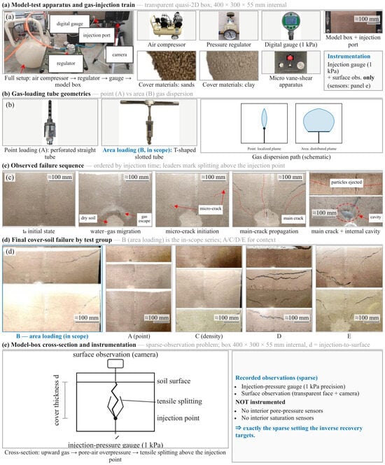
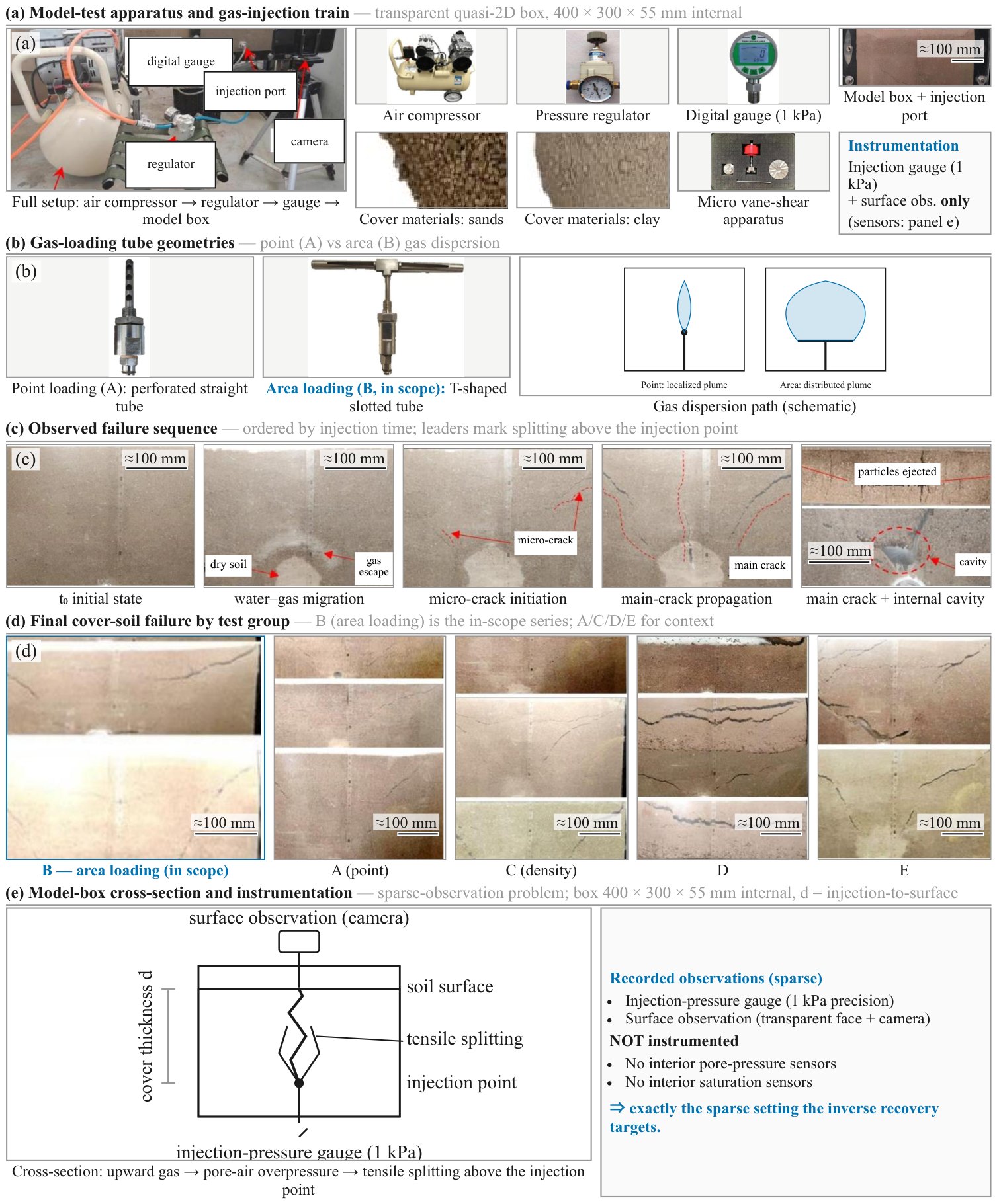
The engineering scenario is anchored in an in-house plane model test that reproduces gas-pressure-induced failure of unsaturated cover soil under controlled conditions, sketched in Figure 1. The apparatus, the loading programme and the two-phase FLAC2D model that supplies the numerical reference fields are our own earlier published work [42]; the present paper takes them as the setting for an inverse-recovery method and does not re-derive them. A sand layer is compacted to a target thickness d and density inside a rigid transparent box, so the deformation stays essentially planar; gas is injected from below through a buried tube while the free surface drains to the atmosphere, and the injected pressure plays the role that trapped biogas plays in the field. Gas is dispersed across a horizontal plane beneath the cover by a T-shaped tube, and the present study uses the cm group. The injection pressure is raised in stages until the cover soil splits along a crack that opens above the injection point.
Figure 1.
The in-house gas-pressure plane model test records the injection pressure and the surface, and nothing inside the soil. A sand cover of thickness d is built in a transparent plane box and loaded from below by an injection tube that disperses gas across a horizontal plane; the instrumentation is an injection-pressure gauge and surface observation only, with no internal pore-pressure sensors. In panel (c), red arrows and dashed outlines identify gas escape, crack development, and cavity formation. The images are ordered by injection time from left to right.
A defining feature of the apparatus is what it does not record. The test reports only the injection-regulator gauge pressure and a surface observation of the failure; it carries no pore-pressure or saturation sensors inside the soil, so the transient field that drives the failure is never observed directly. That absence is the sparse-observation setting this paper addresses.
2.3. The Sparse-Observation Inverse Problem and Its Scope
The transient fields used in the plane-model case are the as-digitised outputs of the companion two-dimensional two-phase FLAC2D simulation reported with the test [42]; they are not in-soil measurements, and no measured interior quantity enters the recovery. That simulation permits gas and water redistribution in the plane, including lateral transport away from the injection zone. In contrast, the inverse model used here enforces one-dimensional vertical balances and contains no lateral flux-divergence term. The case is therefore treated as a deliberately reduced, dimensionally mismatched fit at the three sampled depths. Its training-depth errors test whether the one-dimensional inverse representation can follow those numerical time series; they do not validate the one-dimensional residual against the full two-dimensional field or establish an experimental reconstruction. This distinction also prevents the numerical outputs from being described as sensors.
The numerical evidence is not interchangeable. The one-dimensional finite-volume benchmark solves the same balances as the PINN residual and supplies dense synthetic truth for a self-consistency check. The plane-model case uses three training-depth series from a separate two-dimensional solver and therefore tests a reduced-model fit under the mismatch just described, with no held-out depth in that case. Our earlier field-scale model also provides a vertical transect, line M, through a gas-application zone at depth in an profile. Section 4.4 uses three of its 14 depths for training and the remaining 11 for testing, but without the two-phase residual; it is consequently a held-out depth-interpolation check of the architecture alone. Within these bounds, the method is demonstrated as numerical inverse recovery and the effective-stress post-process is an engineering interpretation of the recovered fields, not a stability calculation.
3. Coupled Water–Air Two-Phase Inverse PINN Methodology
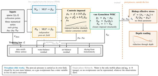
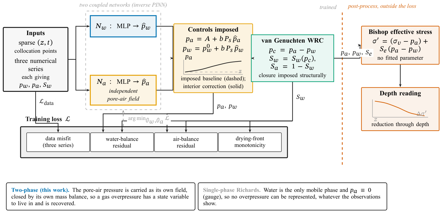
Physics-informed neural networks recover hidden fields by training a network to match sparse observations while satisfying the governing equations as a soft constraint, evaluated by automatic differentiation [1]. For unsaturated flow this idea has been carried furthest in the single-phase Richardson–Richards inverse PINN line, which infers the water-retention and hydraulic-conductivity functions, and the soil-water flux, from volumetric water content alone [11], and which recovers the moisture field and its unspecified boundary conditions from sparse soil-moisture data using domain decomposition [12]. That line transports water only: pore air is held at atmospheric pressure and never enters the residual, so a gas overpressure is invisible to it. The method developed here keeps the inverse, sparse-observation character of that work but adds the missing physics. It carries the pore-air pressure as an independent field governed by its own mass balance and maps the recovered fields onto an effective-stress reading. Figure 2 shows the architecture; the contrast with the single-phase baseline, which recovers no gas overpressure, is the design difference that the rest of this section makes precise.
Figure 2.
Architecture of the coupled water–air two-phase inverse PINN. Carrying the pore-air pressure as an independent field closed by its own mass balance is what makes a gas overpressure representable: the single-phase Richardson–Richards inverse baseline transports water alone and holds no state variable in which one can live. The Bishop effective-stress reduction is computed after training and adds no fitted parameter.
3.1. Coupled Water–Air Two-Phase Flow
Two coupled mass balances govern the column, with the pore-air pressure carried as a primary unknown alongside the pore-water pressure. All pressures are gauge values relative to the atmosphere. Water is treated as incompressible, so its balance conserves the water-filled pore volume,
while the air is compressible, so its balance conserves air mass,
Here n is porosity and z the upward coordinate. The two fluxes share one Darcy mobility expressed through the saturated hydraulic conductivity: for water and for air. Here k is the intrinsic permeability and the water-to-air viscosity ratio, so both flux laws are dimensionally consistent and gravity is retained on both phases. The balances are closed by three relations. Water and air fill the pore space, so the saturations are complementary,
imposed structurally by setting so the closure holds by construction. Matric suction is the pressure difference between the phases: . The air, taken as isothermal and ideal, has density set by the absolute pressure:
with the density at atmospheric pressure , so when the gauge pressure is zero. The retention and relative-permeability behaviour follows the van Genuchten–Mualem model [43,44]. The effective saturation
with for , sets the water saturation as , where is the residual saturation and the inverse air-entry pressure. The water and air mobilities follow the Mualem relations
3.2. Effective Stress and the Configuration-Specific Onset Diagnostic
An effective-stress relation governs how the recovered fields become an onset reading, evaluated entirely outside training so the flow inverse stabilises first. The overburden supplies the total vertical stress , with being the depth below the free surface at . For unsaturated soil the load carried by the skeleton is the average skeleton, or Bishop, effective stress [23], in which the pore pressure is weighted between the air and water phases by an effective-stress parameter tied to the degree of saturation [30,31]. The form of is a constitutive choice, ranging from effective-saturation weighting to the suction–ratio relationship of Khalili and Khabbaz [28] and the suction–stress characteristic curve of Lu and Likos [26], Lu et al. [27]. We use the effective saturation as the baseline closure:
where the gas overpressure enters twice—it lowers the net stress directly and changes the suction term as saturation changes. The baseline is transparent because it uses the saturation already represented through Equation (5) and introduces no additional fitted parameter. The available numerical fields contain no soil-specific effective-stress or shear-strength measurements with which to select one law, so this baseline is not a material-specific calibration.
The zero crossing evaluated here is a configuration-specific diagnostic of loss of vertical effective confinement. The model test builds its cover inside a rigid box and raises the injection pressure until the cover splits along a crack above the injection point (Section 2.2). The rigid sidewalls provide lateral confinement, and the crack location links the diagnostic to the vertical stress carried by the skeleton above the injection source. For this loading path, the onset is read at the injection boundary:
with being the injection boundary. The initial value of this diagnostic depends on the geostatic stress, the initial pore pressures, and the selected law. We evaluate the base instead of a whole-column minimum because the total stress vanishes at the free surface; a gauge overpressure there makes that minimum non-positive from the first instant and reports the boundary condition rather than the injection transient. Reading the injection base avoids that free-surface artifact and follows the crack origin in the confined test, but it does not define a general slope-failure criterion, a slip surface, or a factor of safety. Applied to the recovered fields, the post-process gives the effective-stress reduction through depth, which Section 4.4 evaluates against a dense reference, and the configuration-specific onset time of Equation (8), which Section 4.5 reports across three forms of .
3.3. Inverse PINN Formulation
Two independent networks determine the recovered interior fields. A network outputs the pore-water pressure and a second network outputs the independent pore-air pressure, each a function of the normalised coordinates and . The water saturation is a derived quantity: it follows from the recovered suction through Equation (5), which enforces the closure of Equation (3) automatically. On the one-dimensional benchmark, the prescribed boundary and initial conditions are written into the fields through an ansatz rather than learned:
The injection term carries the basal ramp to the atmospheric top. The ramp time is , the water-pressure baseline is the initial suction head , and the pressure scale is . The bump vanishes at , , and . The ansatz therefore enforces the benchmark boundary and initial conditions exactly. The pore air follows a Dirichlet ramp from 0 to at the base and an atmospheric gauge value at the free-draining top, while the pore water is held at the constant suction head at both ends; the whole column starts from the uniform initial suction at . The interior is left to the networks under the sparse numerical samples and the residuals, and the controlling values , , and T are listed in Table 1. On the plane-model case the only imposed condition is the digitised initial state: and likewise for . The boundaries are inferred from the sampled series and the one-dimensional residuals rather than prescribed. Because the source simulation is two-dimensional, those residuals are a reduced vertical representation and do not include the source model’s lateral transport. The per-setting values are listed in Table 1. Training minimises a composite objective:
The data term sums three mean-squared misfits, one each for pore-air pressure, pore-water pressure, and water saturation at the sampled depths of Table 1. Pressure differences are scaled by , and saturation differences are dimensionless. Each numerical series supplies all three quantities at 41 times across the 20 window, one every 30 , in both settings. The saturation target is supplied separately to the loss, while the predicted saturation follows from the predicted suction through Equation (5). The one-dimensional targets are sampled from the same-equation reference solution. In the plane-model case, the three quantities are digitised separately from the two-dimensional simulation and are not exactly consistent with the retention curve imposed in the inverse model. Separate loss terms therefore do not imply statistically independent observations. Section 4.2 reports the pore-air-pressure fit.
Table 1.
Material, constitutive, and training parameters of the two settings that carry the two-phase residuals. The held-out check of Section 4.4 imposes no constitutive model and therefore takes none of these parameters.
The residual terms and are the mean-squared residuals of Equations (1) and (2) at interior collocation points, each normalised by a characteristic storage rate, and penalises any reversal of the advancing drying front through . The air residual is the term that makes the pore-air pressure a transported field rather than a free interpolant, and it is what distinguishes the formulation from the single-phase baseline of Figure 2. The onset diagnostic of Section 3.2 is a post-process and is absent from by design.
3.4. Training and Reproducibility
A two-stage schedule and a single parameter set drive every run, so the formulation is reproduced rather than re-tuned per case. Because a sharp gas front and a sharp drying front advance together, the doubled residual system is stiff, and the air residual is ramped in only after a short data-and-water warmup of fifteen per cent of the Adam iterations. A first stage of Adam establishes a physically consistent field, after which L-BFGS with a strong-Wolfe line search refines it over the fixed iteration budget of Table 1; collocation points are sampled across the space–time domain, the gradient norm is clipped, and any step returning a non-finite loss at the moving front is skipped. The formulation is applied to the plane-model numerical series only after it clears a self-consistency check on the one-dimensional column—a bounded saturation, a monotone drying front, and a recovered gas-pressure field that reproduces the same-equation reference; that check is reported in Section 4. The same two networks and the same two-stage schedule serve both settings that carry the two-phase residuals, at the per-setting ansatz form, iteration counts, monotonicity weight and pressure scale listed in Table 1.
The reference fields of that one-dimensional column are produced by a forward solve of the same two mass balances, Equations (1) and (2), under the parameters of Table 1: 201 cell-centred finite-volume cells in depth; backward-Euler time stepping on an adaptive step that starts at , grows on easy convergence to a cap of 20 and halves on a failed step down to a floor of 1.0 × 10⁻⁴ ; and a full Newton solve at each step to a storage-scaled residual norm below within at most thirty iterations. The solve advances in 87 accepted steps and 346 Newton iterations and is written out at 81 equally spaced times, from which both the dense fields and the three sparse numerical series are extracted. Because the reference and the residual solve the same system, the one-dimensional column verifies only that the inverse machinery recovers a self-consistent two-phase target. The plane-model series of Section 4.2 come from a separate two-dimensional solver; applying the one-dimensional residual to them omits lateral flux divergence and is assessed only by fit at the sampled depths. The material and constitutive parameters are the set reported for this sand in the prior work on the same apparatus [42], and both settings use them unchanged; the inversion calibrates none of them, which is what the pre-calibrated condition in the results means. Table 1 collects them together with the training parameters of both settings.
3.5. Error Measures
Every error reported in Section 4 is a relative measure, , taken over the discrete support named with the number and weighting every node of that support equally. The normalisation is the reference’s own norm, so each value is read against the quantity it is computed on rather than across quantities: the pore-air pressure is a gauge value that carries a non-zero baseline on the plane-model setting, the water saturation is bounded between and unity, and the Bishop effective stress changes sign. Four further measures carry specific results. The excess error for a sampled series keeps that numerator and normalises by the overpressure above the initial baseline instead——so a series is credited for the transient it develops and not for its baseline; it is undefined where a series stays at that baseline. The maximum per-series error is the largest of the three full-series relative errors, baseline included. The spatial violation fraction measures the drying front: it is the most negative depthwise increment of anywhere on the recovered grid, divided by the saturation range of that field, so it reports the fraction of that range by which monotonicity is broken at its worst point. The recovered-field shift compares two recoveries rather than a recovery and a reference, as the relative distance between the pore-air field recovered under a perturbed parameter and the field recovered at the calibrated values on the common grid. Finally, the effective-stress reduction of Section 4.4 is the drop from the initial state, for , and its error is reported separately from that of the full field.
4. Numerical Benchmarks and Sparse-Observation Inverse Recovery
The evidence in this section is staged according to what each numerical case can establish. A one-dimensional column tests recovery of a self-consistent target generated from the same equations. The plane-model series then test training-depth fit when the one-dimensional residual is applied to output from a separate two-dimensional simulation, under known dimensional and transport mismatch. Ablations identify what the residuals and the independent air field contribute on the one-dimensional benchmark. Finally, line M provides a held-out depth-interpolation check of the architecture alone, without the two-phase residual. These cases are reported separately rather than combined as equivalent validation. All errors below are the relative measures defined in Section 3.5, each read against the quantity and the support named with it.
4.1. Two-Phase Recovery on the One-Dimensional Benchmark
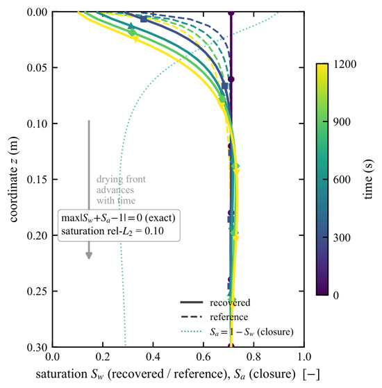
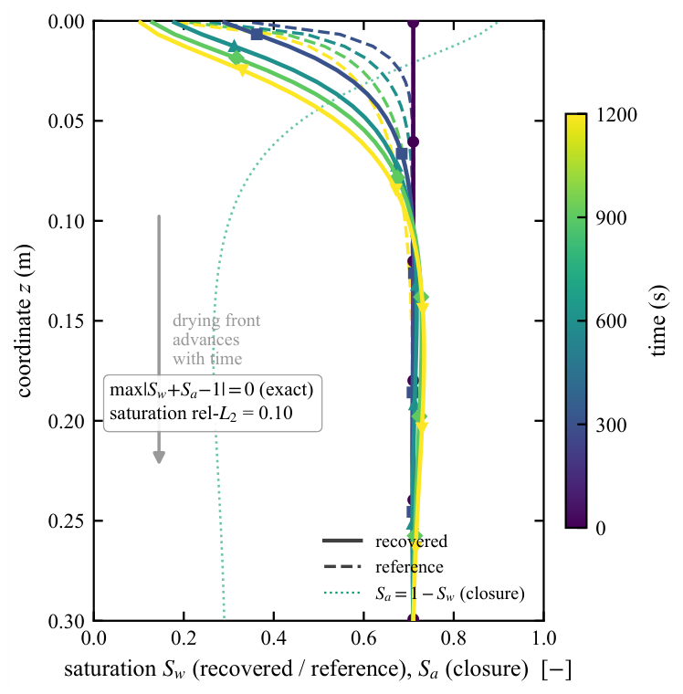
On the one-dimensional column the recovered saturation remains bounded throughout the dense reference domain. Within the structural closure , which holds by construction because the air saturation is set as the complement of the water saturation, the recovered water-saturation profiles track the reference inside its physical range throughout the time window, and the drying front advances monotonically, with a spatial violation fraction of 0.00058 and no temporal reversal, at a saturation relative error of 0.10 over the dense reference, saturation being among the three sampled quantities (Figure 3). The recovered gas-pressure field reproduces the dense reference at a relative error of 0.0463. Two conditions frame that figure. The reference solves the same two mass balances the residual enforces (Section 3.4), so the agreement is a self-consistency test rather than independent physical validation; and the boundary and initial controls are imposed exactly through the ansatz of Equation (9), so the network supplies the interior correction between the sampled depths. That correction accounts for a measurable share of the agreement: with the pore-air network output suppressed, the imposed basal ramp alone reproduces the dense reference at a relative error of 0.0755, and the trained interior correction brings the field to 0.0463.
Figure 3.
Recovered water-saturation profiles on the one-dimensional benchmark. Profiles along z at five injection times (recovered, solid; reference, dashed) stay within the physical range while the drying front advances monotonically; the saturation relative error is 0.10. The coordinate z is measured upward from the injection base. Circles, squares, upward triangles, diamonds, and downward triangles mark the recovered profiles at 0, 300, 600, 900, and 1200 s, respectively; colours encode the same times. The dotted grey curve shows the complementary air saturation at 1200 s.
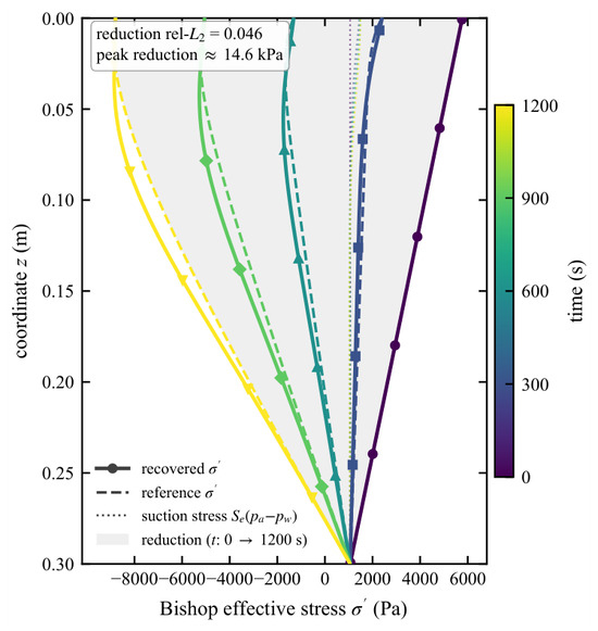
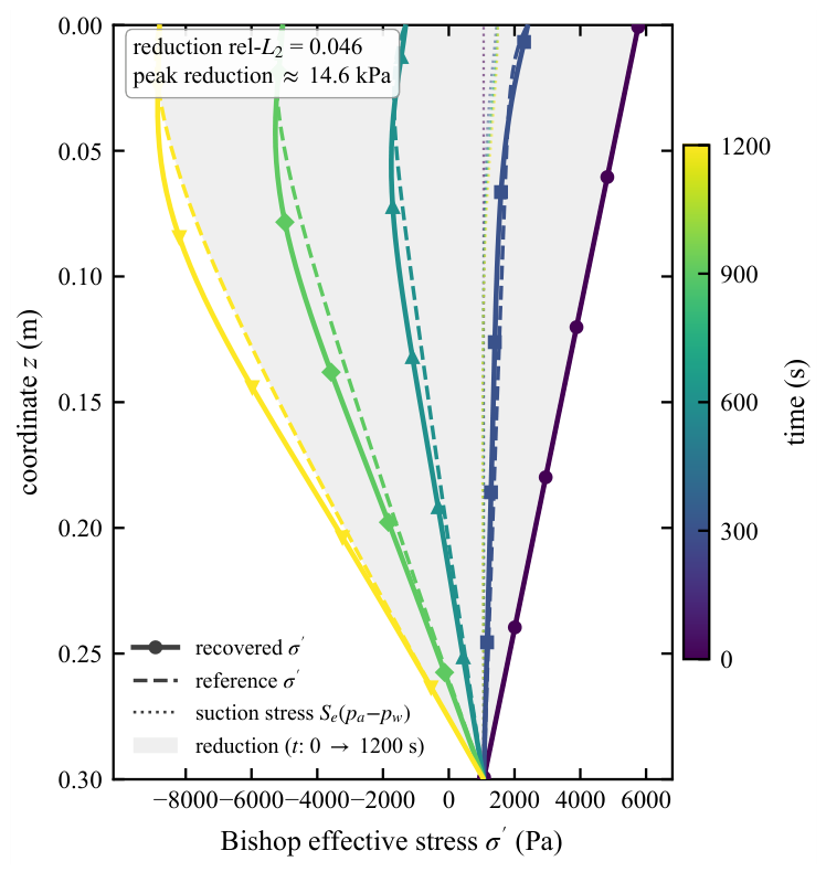
The benchmark also separates a physically interpretable interval from an overload stress test. In the reference field, the injection-base Bishop effective stress first becomes non-positive at 495 s; the preceding saved state is 480 s. Over the pre-onset interval s, the recovered gas-pressure field has a relative error of 0.0448. Restricting that interval further to cells with positive reference effective stress gives a gas-pressure error of 0.0453 and an effective-stress-reduction error of 0.0450. These errors remain close to the respective full-window values of 0.0463 and 0.0459 while the rigid-skeleton assumptions apply. From 495 s onward, the fixed porosity and geostatic total stress no longer represent the mechanical response. The full-window values therefore describe numerical recovery under strong forcing. The final reference value of about kPa belongs to that overload test; post-failure stress prediction requires a deformable-skeleton model.
4.2. Sparse-Observation Recovery of the Transient Pore-Air-Pressure Field
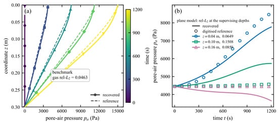
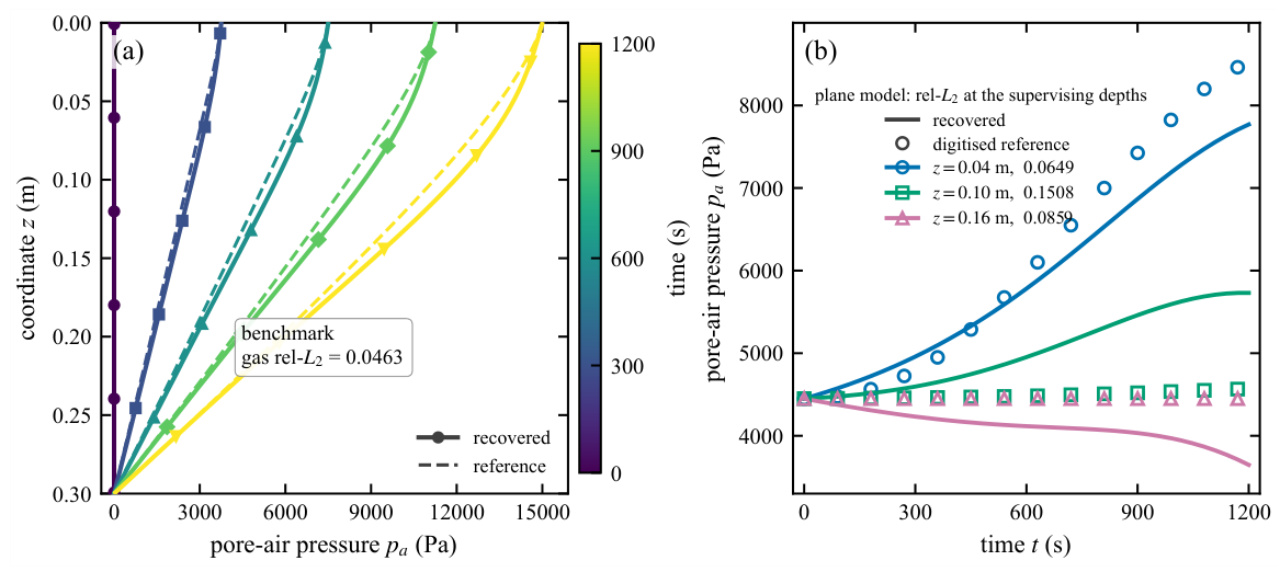
On the one-dimensional benchmark, the recovered profiles follow the dense same-equation reference at a relative error of 0.0463 (Figure 4a). The plane-model case has a different role. Its target series are transient pore-air pressures digitised from the companion two-dimensional two-phase simulation of the cm gas-injection group, at depths of 0.04, 0.10, and 0.16 m in the 0.20 m cover. The one-dimensional inverse model reproduces those three training series at relative errors of 0.0649, 0.1508, and 0.0859 (Figure 4b). These are fit residuals at the sampled depths, not held-out errors or a comparison over the two-dimensional field. In particular, lateral gas and water redistribution present in the FLAC2D source is absent from the residual, so agreement at the three depths demonstrates reduced-model tracking of the supplied series rather than validation of a one-dimensional transport assumption. The two shallower series remain close to their initial baseline and their full-series errors are therefore baseline-dominated; the deepest series has the strongest transient, with an overpressure-above-baseline excess error of 0.186. Across a five-seed ensemble the per-series error spread stays below a standard deviation of 0.0007.
Figure 4.
Recovered transient pore-air pressure. (a) One-dimensional benchmark profiles, recovered (solid) against the same-equation reference (dashed); relative error 0.0463. Circles, squares, upward triangles, diamonds, and downward triangles mark the recovered profiles at 0, 300, 600, 900, and 1200 s, respectively; colours encode the same times. (b) Three target series digitised from the companion two-dimensional plane-model simulation (markers) against the one-dimensional reconstruction (lines); per-series relative errors 0.0649, 0.1508, and 0.0859. Blue circles, green squares, and magenta upward triangles denote the reference series at , , and m, respectively; the solid curves use the corresponding colours. Panel (b) reports fit at the three training depths under dimensional mismatch, not held-out or full-field validation.
4.3. Ablations and the Single-Phase Baseline
The gas overpressure is visible to the inversion because the pore-air pressure is an independent field. The single-phase Richards baseline, which transports water alone and holds the pore air at its constant initial value, recovers no overpressure: its excess error for the responding series is 1.0, against 0.186 for the two-phase model on the same series. This comparison establishes representability. It is separate from the accuracy contribution of the residuals. Removing the air mass-balance residual while keeping the air field raises the one-dimensional gas-pressure error from 0.0463 to 0.1328, whereas removing every residual lowers it to 0.0043. The loss terms therefore do not provide additive improvements to the gas-pressure metric. The data-only network is optimized for the sampled state values alone; the full model must also satisfy the coupled water and air balances through one retention relation. On this benchmark, whose injection ramp is imposed exactly and whose three series supervise the field, that joint constraint worsens the gas-pressure error while improving the other state variables.
With every residual removed, the pore-water error grows from 0.2307 to 0.4898 and the interior saturation error from 0.100 to 0.243. The drying front also ceases to advance monotonically: its spatial violation fraction rises from 0.00058 to 0.0315, and the data-only variant is the one case of the four in which the front reverses. With the explicit monotonicity penalty removed and the residuals retained, the front remains monotone at the full-model level, with a spatial violation fraction of 0.00048 against 0.00058. The coupled residuals are therefore retained for the conservation-consistent joint pore-air, pore-water, and saturation state. The independent air field supplies representability; the residuals supply the physical coupling around that field.
4.4. Bishop Effective-Stress Reduction as a Parameter-Free Post-Process
The effective-stress consequence of the recovered fields follows without any additional fitted parameter, through evaluated on the recovered . Over the full numerical window, the recovered effective-stress reduction agrees with the one-dimensional reference at a relative error of 0.0459 (Figure 5), and the full field at 0.0834. The reduction inherits the gas-field accuracy because the transient reduction is dominated by the pore-air overpressure term; the suction-stress component, which depends on the weaker reconstruction, contributes an error of 0.0556. Within the physically applicable subset defined in Section 4.1, before the 495 s injection-base crossing and where the reference remains positive, the reduction error is 0.0450. The post-crossing profiles assess numerical tracking under overload; post-failure stress prediction requires a deformable-skeleton model.
Figure 5.
Recovered Bishop effective-stress reduction on the one-dimensional benchmark. Profiles of effective stress along z at five times (recovered, solid; parameter-free reference from the ground-truth fields, dashed) with the suction-stress component overlaid. Circles, squares, upward triangles, diamonds, and downward triangles mark the recovered profiles at 0, 300, 600, 900, and 1200 s, respectively; colours encode the same times. Dotted curves show the suction-stress component, and the shaded region shows the reference effective-stress reduction from 0 to 1200 s. The reduction error is 0.0450 before the 495 s injection-base crossing on cells with positive reference , and 0.0459 over the full numerical window. The post-onset profiles display numerical tracking under overload.
One held-out check stands outside the two-phase formulation. On the line-M transect of Section 2.3, the same network architecture is trained on three of the 14 digitised depths and evaluated on the other 11, without the two-phase residuals. Those residuals are absent by construction: the digitised triples of that model are not van Genuchten consistent with the column air-entry value, so imposing the column constitutive coupling on them would be inappropriate. The held-out relative error is 0.1173 when one of the three training depths coincides with the gas-application depth of 5.5 m, and 0.332 under a blind-uniform three-depth layout that omits it, because the sharp gas-pressure peak lies above its flanking samples. This case therefore measures architecture-only depth interpolation and the importance of sampling the loading zone; unlike the plane-model case, its reported errors are held out, but unlike the benchmark and plane-model cases it does not test the two-phase PINN formulation.
4.5. Robustness of the Inverse Recovery
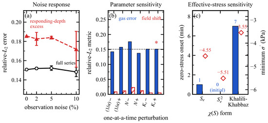
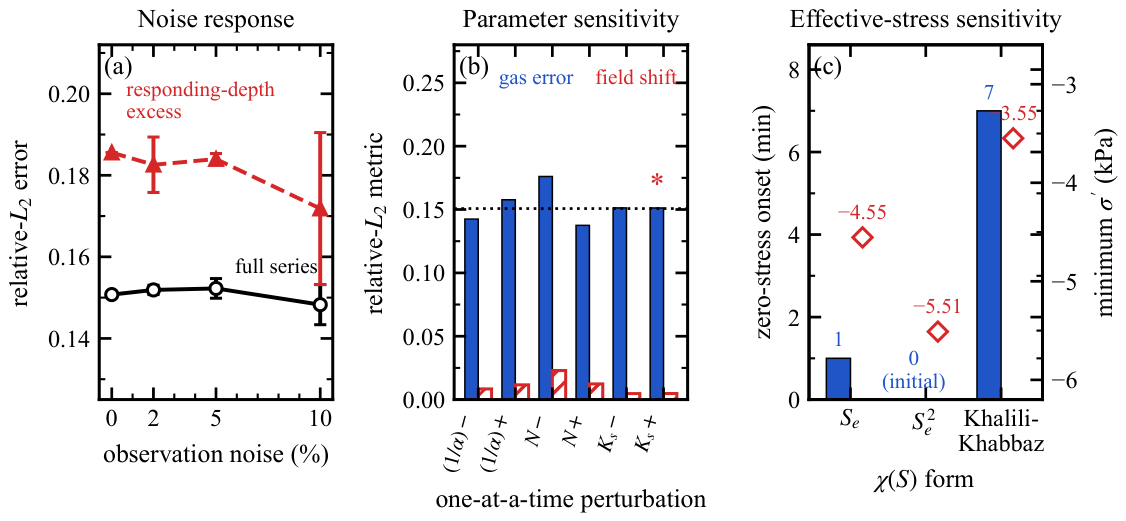
Three further studies bound how far the recovered fields can be trusted: their behaviour under observation noise, under a one-at-a-time perturbation of the van Genuchten retention parameters and the saturated conductivity, and under the Bishop effective-stress form used in the post-process (Figure 6). Each reports where a conclusion holds and where a quantity becomes choice-dependent.
Figure 6.
Robustness and sensitivity of the inverse recovery on the plane-model setting. (a) Full-series and responding-depth excess-overpressure errors versus observation noise (three-seed mean ± standard deviation). (b) Maximum gas error and recovered-field shift under one-at-a-time constitutive-parameter perturbations of air-entry pressure , van Genuchten N, and saturated conductivity . The asterisk marks the non-converged diagnostic, which is excluded from the converged range; the dotted line gives the baseline gas error. (c) Injection-base zero-stress time and minimum effective stress for three Bishop forms applied to the same recovered fields; their zero-to-seven-minute timing and 43% minimum-stress spread define a model-form envelope, with retained as the uncalibrated baseline. Blue bars use the left axis for onset time; red open diamonds use the right axis for minimum effective stress.
The reconstruction stays stable under the tested observation noise. Adding zero-mean noise at two, five, and ten per cent of the dominant overpressure amplitude leaves the three-seed mean maximum full-series error at 0.152, 0.152, and 0.148, respectively, against 0.151 for the clean run (Figure 6a). This metric is set by the baseline-dominated shallow numerical series described in Section 4.2. The responding-depth excess-overpressure error measures the transient signal directly: its three-seed mean is 0.183, 0.184, and 0.172 at the same noise levels, against 0.186 for the clean run; the corresponding standard deviations are 0.0068, 0.0013, and 0.0186. Excess-relative errors are not reported at the other two depths because their near-zero excess-pressure denominators are ill-conditioned or undefined. Noise also reaches the interior solution: drying-front monotonicity, an auxiliary soft regulariser rather than the recovery metric, relaxes in a minority of seeds at the higher noise levels while the pressure and saturation bounds remain satisfied.
The one-at-a-time parameter study measures sensitivity to constitutive misspecification, not parameter identifiability. Among the five converged perturbations of the air-entry value, the van Genuchten N, and the saturated conductivity, the maximum gas error ranges from 0.138 to 0.176 and the recovered pore-air field shifts by less than 2.3 per cent in relative from the baseline recovery (Figure 6b). The van Genuchten N produces the largest shift. The run gives a diagnostic gas-error value of 0.1512 and a field shift of 0.0048, but it fails the declared convergence assessment because the recovered drying front is non-monotone (spatial and temporal violation fractions 0.00732 and 0.04497). Figure 6b marks this value separately, and it is excluded from the converged sensitivity range.
The Bishop form has a larger effect on the effective-stress interpretation. Three forms are applied to the same recovered fields without retraining: , , and the Khalili–Khabbaz form [28] (Figure 6c). All three make the injection-base effective stress non-positive, so the direction of the response is form-robust for this confined loading configuration. The form controls the numerical threshold: the first non-positive sample ranges from zero to seven minutes, and the minimum effective stress ranges from to kPa, a spread of 1.96 kPa or about 43 per cent of the baseline magnitude. The zero-minute result under occurs because the changed suction weighting makes the initial injection-base value non-positive, which demonstrates the diagnostic’s dependence on both the law and the initial pressure state. The curve is retained as a transparent baseline, not a uniquely selected law for this sand. A quantitative engineering threshold would require soil-specific calibration of the effective-stress or suction-dependent strength relation; without that calibration, the three forms define a model-form envelope for timing and severity.
5. Discussion
Within this numerical proof of concept, the transient gas overpressure can be represented only when the pore-air pressure is carried as an independent transported field rather than inferred from the water phase. The strength of the evidence depends on the case: same-equation dense recovery on the one-dimensional benchmark, training-depth tracking under one-dimensional/two-dimensional model mismatch on the plane-model series, and architecture-only held-out interpolation on line M. The Discussion therefore separates the formulation result from the engineering interpretation supplied by the effective-stress post-process.
5.1. The Independent Air Phase
The single-phase Richardson–Richards inverse line transports water alone and holds the pore air at atmospheric pressure [11,12]. That formulation is well founded for infiltration problems, but it carries no state variable in which a gas overpressure can live, so the quantity this paper needs is invisible to it by construction. The two-phase extension supplies that missing variable. A single-phase Richards baseline, given the same pore-water observations, recovers no gas overpressure, which follows from the formulation itself. The empirical question is what the mass balances add once the variable exists, and the ablations of Section 4.3 give an adverse but informative answer. On a benchmark whose injection history is written into the ansatz and whose three numerical series supervise the fit, the data-only network gives a gas-pressure error of 0.0043, compared with 0.0463 for the full model. The coupled residuals improve the pore-water and saturation errors and prevent reversal of the drying front. Their measured contribution is a conservation-constrained joint state. This field-level numerical target also separates the method from the closest inverse multiphase PINN, which recovers lumped poromechanical parameters from dense data rather than a transient pore-air field from sparse observations [15].
5.2. The Conservation Residual and the Effective-Stress Post-Process
The governing residual holds the monotone advance of the recovered front. The delivered loss also includes the explicit monotonicity penalty of Equation (10) at the weight of Table 1, and the ablation of Section 4.3 measures the residual to be sufficient without it. Section 4.3 separates that result from the role of the independent air field: the water balance alone can regularise the front, whereas the air field is the state variable that carries overpressure. Reaching the coupled recovery required conditioning the optimisation for a stiff, doubled residual system: the air balance is introduced after a short data-and-water warmup, each residual is normalised by a characteristic storage rate, and the controlled boundary and initial conditions are written into the fields through an ansatz rather than learned.
The Bishop effective-stress reduction is then a post-process of that joint state. Within the one-dimensional benchmark’s applicable interval, it agrees with the reference reduction at 0.0450 on positive-reference-stress cells. The injection-base zero crossing is interpreted only for the laterally confined cover and the observed crack location above the gas source. Its timing and severity depend strongly on and the initial pressure state, so the three tested forms provide an uncertainty envelope rather than a transferable threshold. Selection of a quantitative law for another soil or a slope requires effective-stress or suction-dependent strength calibration for that material and stress path.
Related mappings from spatial data to mechanical quantities include laboratory-scale estimates of elastic modulus and permeability from grout-vein geometry extracted from images [45] and multi-modal neural-operator reconstruction of rock-damage fields from discrete-element particle states [46].
5.3. Limitations
Three evidence limits fix what this demonstration reaches. First, the dense one-dimensional benchmark is generated from the same equations as the PINN residual and therefore establishes self-consistency, not independent physical validity. Second, the plane-model reference is two-dimensional and includes lateral transport, whereas the inverse residual is one-dimensional; its reported errors are training-depth fits under model mismatch, with no held-out depth or full-field comparison. Third, the line-M check holds out 11 of 14 depths but removes the two-phase residual, so it tests the network architecture rather than the coupled formulation. None of the cases use measured interior pore-air pressure or saturation. The object studied here is a gas-loaded unsaturated cover soil: a one-dimensional column, numerical series associated with a plane cover in a rigid box, and a vertical transect through a two-dimensional model. No slope stability analysis is performed, and the study carries no slope geometry, slip surface, deformation or factor of safety. The landfill and fill-slope setting of Section 2.1 motivates the mechanism; applying the recovered fields in a stability assessment remains a downstream task that would require mechanical parameters and a stability model. The one-dimensional benchmark uses a rigid skeleton, fixed porosity, and geostatic total stress. Physical interpretation is therefore restricted to the pre-onset interval ending at the 495 s reference injection-base crossing and to cells with positive reference effective stress. The later profiles test whether the inverse and post-process continue to track their numerical reference under overload; they do not describe post-failure deformation or stress redistribution.
Extensions to failure require flow–solid coupling and material-specific characterisation. Related rock-engineering examples include CFD–DEM coupling of slurry flow and rock-particle breakage in a TBM jaw crusher [47] and measurements of bedding-dependent Mode III fracture toughness in layered sandstone [48].
Field use of the demonstrated data term requires pore-air pressure, pore-water pressure, and water saturation at the observation depths and times. Saturation can be measured independently or estimated from the measured suction using an independently calibrated water-retention relation applicable to the soil and loading path. In the latter case, saturation provides a constitutive constraint derived from the pressure observations, with correlated measurement errors and uncertainty from the retention parameters. The loss weights would need to account for those dependencies; the present numerical results use separately supplied saturation targets and do not test this pressure-derived observation scheme.
6. Conclusions
This numerical proof of concept reconstructs transient pore-air-pressure fields in unsaturated cover soils with a coupled water–air inverse physics-informed neural network and computes their Bishop effective-stress reduction. The two-phase formulation uses a pre-calibrated constitutive model and separately supplies pore-air pressure, pore-water pressure, and saturation targets at three numerically sampled depths. Its independent pore-air field makes overpressure representable, and the coupled mass balances constrain the joint state.
The data-only ablation gives the lowest one-dimensional gas-pressure error, 0.0043, while the coupled residuals improve the pore-water and saturation fields and retain a monotone drying front. The residuals contribute a conservation-constrained joint state. Before the reference injection-base effective stress first becomes non-positive at 495 s, the gas-pressure error is 0.0448; on the positive-reference-stress cells in that interval, the effective-stress-reduction error is 0.0450. Later states form a numerical overload stress test. Across three forms, the confined-cover injection base reaches zero effective stress, but the zero-to-seven-minute timing and 43% minimum-stress spread are constitutive-model uncertainty. A transferable quantitative threshold requires soil-specific effective-stress or strength calibration.
The two further numerical cases provide distinct evidence. The plane-model case fits three training-depth series from a two-dimensional FLAC2D calculation with a one-dimensional residual that omits lateral transport; its responding-depth excess-overpressure fit error is 0.186. The line-M case evaluates interpolation at 11 held-out depths using the network architecture without the two-phase residual. The latter tests the architecture’s interpolation capability, while the former measures training-depth fit under dimensional mismatch.
The Bishop calculation provides a depth-resolved, configuration-specific effective-stress post-process of the recovered numerical fields. Field application requires pore-air pressure, pore-water pressure, and saturation observations; saturation may be measured independently or derived from suction through an independently calibrated retention relation applicable to the soil and loading path, with the correlated errors and parameter uncertainty treated as described in Section 5.3. Using the recovered fields in a stability assessment additionally requires soil-specific effective-stress or strength calibration and a mechanical model for deformation and failure.
Author Contributions
Conceptualisation, J.P.; methodology, P.Z.; software, P.Z.; validation, P.Z.; formal analysis, P.Z.; investigation, J.P. and M.Y.; resources, M.Y.; data curation, M.Y.; visualisation, P.Z.; writing—original draft preparation, J.P. and P.Z.; writing—review and editing, T.C.; supervision, T.C.; project administration, T.C. All authors have read and agreed to the published version of the manuscript.
Funding
This research received no external funding.
Institutional Review Board Statement
Not applicable.
Informed Consent Statement
Not applicable.
Data Availability Statement
The original contributions presented in this study are included in the article. Further inquiries can be directed to the corresponding authors.
Acknowledgments
The authors thank the Key Laboratory of Urban Underground Engineering of Ministry of Education, Beijing Jiaotong University, for providing experimental facilities and support.
Conflicts of Interest
Author Jiaqiang Peng is affiliated with PowerChina Roadbridge Group Co., Ltd. as his second affiliation. Author Maohong Yao was employed by PowerChina Chengdu Engineering Co., Ltd. The remaining authors declare that the research was conducted in the absence of any commercial or financial relationships that could be construed as a potential conflict of interest.
References
- Raissi, M.; Perdikaris, P.; Karniadakis, G.E. Physics-informed neural networks: A deep learning framework for solving forward and inverse problems involving nonlinear partial differential equations. J. Comput. Phys. 2019, 378, 686–707. [Google Scholar] [CrossRef] [Scilit]
- Karniadakis, G.E.; Kevrekidis, I.G.; Lu, L.; Perdikaris, P.; Wang, S.; Yang, L. Physics-informed machine learning. Nat. Rev. Phys. 2021, 3, 422–440. [Google Scholar] [CrossRef] [Scilit]
- Cuomo, S.; Di Cola, V.S.; Giampaolo, F.; Rozza, G.; Raissi, M.; Piccialli, F. Scientific Machine Learning Through Physics-Informed Neural Networks: Where we are and What’s Next. J. Sci. Comput. 2022, 92, 88. [Google Scholar] [CrossRef] [Scilit]
- Yang, L.; Meng, X.; Karniadakis, G.E. B-PINNs: Bayesian physics-informed neural networks for forward and inverse PDE problems with noisy data. J. Comput. Phys. 2021, 425, 109913. [Google Scholar] [CrossRef] [Scilit]
- Zhang, D.; Lu, L.; Guo, L.; Karniadakis, G.E. Quantifying total uncertainty in physics-informed neural networks for solving forward and inverse stochastic problems. J. Comput. Phys. 2019, 397, 108850. [Google Scholar] [CrossRef] [Scilit]
- Jagtap, A.D.; Kharazmi, E.; Karniadakis, G.E. Conservative physics-informed neural networks on discrete domains for conservation laws: Applications to forward and inverse problems. Comput. Methods Appl. Mech. Eng. 2020, 365, 113028. [Google Scholar] [CrossRef] [Scilit]
- Lu, L.; Meng, X.; Mao, Z.; Karniadakis, G.E. DeepXDE: A Deep Learning Library for Solving Differential Equations. SIAM Rev. 2021, 63, 208–228. [Google Scholar] [CrossRef] [Scilit]
- Wang, Y.; Shi, C.; Shi, J.; Lu, H. Data-driven forward and inverse analysis of two-dimensional soil consolidation using physics-informed neural network. Acta Geotech. 2024, 19, 8051–8069. [Google Scholar] [CrossRef] [Scilit]
- Elbaz, K.; Cai, Q.; Shen, S.L.; Xie, D. TF-PINN model for solving forward and inverse problems during shield tunneling. Acta Geotech. 2025, 20, 5917–5939. [Google Scholar] [CrossRef] [Scilit]
- Berardi, M.; Difonzo, F.V.; Icardi, M. Inverse Physics-Informed Neural Networks for transport models in porous materials. Comput. Methods Appl. Mech. Eng. 2025, 435, 117628. [Google Scholar] [CrossRef] [Scilit]
- Bandai, T.; Ghezzehei, T.A. Physics-Informed Neural Networks with Monotonicity Constraints for Richardson-Richards Equation: Estimation of Constitutive Relationships and Soil Water Flux Density from Volumetric Water Content Measurements. Water Resour. Res. 2021, 57, e2020WR027642. [Google Scholar] [CrossRef] [Scilit]
- Bandai, T.; Ghezzehei, T.A. Forward and inverse modeling of water flow in unsaturated soils with discontinuous hydraulic conductivities using physics-informed neural networks with domain decomposition. Hydrol. Earth Syst. Sci. 2022, 26, 4469–4495. [Google Scholar] [CrossRef] [Scilit]
- Zhang, J.; Braga-Neto, U.; Gildin, E. Physics-informed neural networks for multi-phase flow in porous media considering dual shocks and interphase solubility. arXiv 2024, arXiv:2404.12502. [Google Scholar] [CrossRef] [Scilit]
- Elfetni, S.; Kamachali, R.D. PINNs-MPF: A Physics-Informed Neural Network framework for Multi-Phase-Field simulation of interface dynamics. Eng. Anal. Bound. Elem. 2025, 176, 106200. [Google Scholar] [CrossRef] [Scilit]
- Amini, D.; Haghighat, E.; Juanes, R. Inverse modeling of nonisothermal multiphase poromechanics using physics-informed neural networks. J. Comput. Phys. 2023, 490, 112323. [Google Scholar] [CrossRef] [Scilit]
- Carrera, J.; Neuman, S.P. Estimation of Aquifer Parameters Under Transient and Steady State Conditions: 1. Maximum Likelihood Method Incorporating Prior Information. Water Resour. Res. 1986, 22, 199–210. [Google Scholar] [CrossRef] [Scilit]
- Zhou, H.; Gómez-Hernández, J.J.; Li, L. Inverse methods in hydrogeology: Evolution and recent trends. Adv. Water Resour. 2014, 63, 22–37. [Google Scholar] [CrossRef] [Scilit]
- Evensen, G. The Ensemble Kalman Filter: Theoretical formulation and practical implementation. Ocean Dyn. 2003, 53, 343–367. [Google Scholar] [CrossRef] [Scilit]
- Aanonsen, S.I.; Nævdal, G.; Oliver, D.S.; Reynolds, A.C.; Vallès, B. The Ensemble Kalman Filter in Reservoir Engineering—A Review. SPE J. 2009, 14, 393–412. [Google Scholar] [CrossRef] [Scilit]
- Oliver, D.S.; Chen, Y. Recent progress on reservoir history matching: A review. Comput. Geosci. 2011, 15, 185–221. [Google Scholar] [CrossRef] [Scilit]
- Pensoneault, A.; Zhu, X. Efficient Bayesian physics-informed neural networks for inverse problems via ensemble Kalman inversion. arXiv 2023, arXiv:2303.07392. [Google Scholar] [CrossRef] [Scilit]
- Larion, Y.; Chen, G.; Zlotnik, S.; Díez, P.; Seetharam, S.; Massart, T.J. Using Reduced Basis Approximation for Efficient Surrogate-Based Inverse Identification of Thermo-Hydro-Mechanical Parameters from an In Situ Heating Test. Rock Mech. Rock Eng. 2022, 55, 5739–5757. [Google Scholar] [CrossRef] [Scilit]
- Bishop, A.W.; Blight, G.E. Some Aspects of Effective Stress in Saturated and Partly Saturated Soils. Géotechnique 1963, 13, 177–197. [Google Scholar] [CrossRef] [Scilit]
- Fredlund, D.G.; Morgenstern, N.R. Stress State Variables for Unsaturated Soils. J. Geotech. Eng. Div. 1977, 103, 447–466. [Google Scholar] [CrossRef] [Scilit]
- Fredlund, D.G.; Morgenstern, N.R.; Widger, R.A. The shear strength of unsaturated soils. Can. Geotech. J. 1978, 15, 313–321. [Google Scholar] [CrossRef] [Scilit]
- Lu, N.; Likos, W.J. Suction Stress Characteristic Curve for Unsaturated Soil. J. Geotech. Geoenviron. Eng. 2006, 132, 131–142. [Google Scholar] [CrossRef] [Scilit]
- Lu, N.; Godt, J.W.; Wu, D.T. A closed-form equation for effective stress in unsaturated soil. Water Resour. Res. 2010, 46, W05515. [Google Scholar] [CrossRef] [Scilit]
- Khalili, N.; Khabbaz, M.H. A unique relationship for χ for the determination of the shear strength of unsaturated soils. Géotechnique 1998, 48, 681–687. [Google Scholar] [CrossRef] [Scilit]
- Vanapalli, S.K.; Fredlund, D.G.; Pufahl, D.E.; Clifton, A.W. Model for the prediction of shear strength with respect to soil suction. Can. Geotech. J. 1996, 33, 379–392. [Google Scholar] [CrossRef] [Scilit]
- Gallipoli, D.; Gens, A.; Sharma, R.; Vaunat, J. An elasto-plastic model for unsaturated soil incorporating the effects of suction and degree of saturation on mechanical behaviour. Géotechnique 2003, 53, 123–135. [Google Scholar] [CrossRef]
- Sheng, D.; Fredlund, D.G.; Gens, A. A new modelling approach for unsaturated soils using independent stress variables. Can. Geotech. J. 2008, 45, 511–534. [Google Scholar] [CrossRef] [Scilit]
- McDougall, J. A hydro-bio-mechanical model for settlement and other behaviour in landfilled waste. Comput. Geotech. 2007, 34, 229–246. [Google Scholar] [CrossRef] [Scilit]
- Chen, Y.; Xu, X.; Zhan, L. Analysis of solid-liquid-gas interactions in landfilled municipal solid waste by a bio-hydro-mechanical coupled model. Sci. China Technol. Sci. 2012, 55, 81–89. [Google Scholar] [CrossRef] [Scilit]
- Shu, S.; Li, Y.; Sun, Z.; Shi, J. Effect of gas pressure on municipal solid waste landfill slope stability. Waste Manag. Res. J. A Sustain. Circ. Econ. 2022, 40, 323–330. [Google Scholar] [CrossRef] [Scilit] [PubMed]
- Hu, J.; Chen, Y.M.; Li, J.H.; Ke, H.; Li, J.C. Centrifuge modeling of slope failure induced by elevated gas pressure in wet municipal solid waste landfill. Can. Geotech. J. 2024, 61, 1094–1108. [Google Scholar] [CrossRef] [Scilit]
- Blight, G. Slope failures in municipal solid waste dumps and landfills: A review. Waste Manag. Res. J. A Sustain. Circ. Econ. 2008, 26, 448–463. [Google Scholar] [CrossRef] [Scilit] [PubMed]
- Stark, T.D.; Eid, H.T.; Evans, W.D.; Sherry, P.E. Municipal Solid Waste Slope Failure. II: Stability Analyses. J. Geotech. Geoenviron. Eng. 2000, 126, 408–419. [Google Scholar] [CrossRef] [Scilit]
- Cho, S.E. Stability analysis of unsaturated soil slopes considering water-air flow caused by rainfall infiltration. Eng. Geol. 2016, 211, 184–197. [Google Scholar] [CrossRef] [Scilit]
- Sun, D.M.; Zang, Y.G.; Semprich, S. Effects of Airflow Induced by Rainfall Infiltration on Unsaturated Soil Slope Stability. Transp. Porous Media 2015, 107, 821–841. [Google Scholar] [CrossRef] [Scilit]
- Kang, S.; Cho, S.E.; Kim, B.; Go, G.H. Effects of Two-Phase Flow of Water and Air on Shallow Slope Failures Induced by Rainfall: Insights from Slope Stability Assessment at a Regional Scale. Water 2020, 12, 812. [Google Scholar] [CrossRef] [Scilit]
- Liu, G.; Zha, X.Y.; Guan, J.K.; Tong, F.G. Field experiment of rainfall infiltration on a soil slope and simulations based on a water-air two-phase flow model. J. Mt. Sci. 2021, 18, 2159–2167. [Google Scholar] [CrossRef] [Scilit]
- Yao, M.; Chen, T.; Song, Y.; Zhang, W.; Wang, X.; Xing, X. Dynamic stability analysis of unsaturated slopes triggered by high gas pressure: Critical pressure threshold and progressive failure evolution. J. Mt. Sci. 2025, 22, 2981–2995. [Google Scholar] [CrossRef] [Scilit]
- van Genuchten, M.T. A Closed-form Equation for Predicting the Hydraulic Conductivity of Unsaturated Soils. Soil Sci. Soc. Am. J. 1980, 44, 892–898. [Google Scholar] [CrossRef] [Scilit]
- Mualem, Y. A new model for predicting the hydraulic conductivity of unsaturated porous media. Water Resour. Res. 1976, 12, 513–522. [Google Scholar] [CrossRef] [Scilit]
- Zhu, P.; Zhang, Z.; Chen, T.; Wang, R.; Zhang, D.; Zhu, L.; Guo, J. A width centric image to mechanics framework for assessing advance grouting with TMSE adaptive width segmentation and lab scale validation. Sci. Rep. 2025, 15, 40950. [Google Scholar] [CrossRef] [Scilit] [PubMed]
- Wang, L.; Wang, Y.; Zhu, P.; Chen, T.; Liu, A. Full-field damage reconstruction from discrete-element particle states: A multi-modal neural operator and benchmark for rock direct shear. Comput. Part. Mech. 2026, 17, 246–273. [Google Scholar] [CrossRef] [Scilit]
- Guo, Y.; Li, X.; Ning, F.; Fang, Y.; Liu, H. Case study on jaw crusher rock breaking for slurry TBM using Tavares UFRJ breakage model and coupled CFD-DEM. Undergr. Space 2026, 29, 134–163. [Google Scholar] [CrossRef] [Scilit]
- Zhu, P.; Zhao, H.; He, Y.; Chen, T.; Wang, G.; Yang, S.; Dong, X. True Mode III Fracture Toughness and Bedding-Induced Anisotropy of Layered Sandstone Using ANBD Brazilian Disks. Rock Mech. Rock Eng. 2026. [Google Scholar] [CrossRef] [Scilit]

Disclaimer/Publisher’s Note: The statements, opinions and data contained in all publications are solely those of the individual author(s) and contributor(s) and not of MDPI and/or the editor(s). MDPI and/or the editor(s) disclaim responsibility for any injury to people or property resulting from any ideas, methods, instructions or products referred to in the content. |
© 2026 by the authors. Licensee MDPI, Basel, Switzerland. This article is an open access article distributed under the terms and conditions of the Creative Commons Attribution (CC BY) license.