Estimation of the Limit Slope Equilibrium Based on the Solution of a Geometric Nonlinear Coupled Problem

Abstract

This article addresses the problem of slope stability from two complementary perspectives. On the one hand, it considers practical issues related to improving the efficiency of construction on subsidence soils. On the other hand, since traditional experimental and theoretical methods proved insufficient, it was necessary to develop new methodological tools for solving this class of problems. A method is developed for calculating slope stability without predefining the shape of the failure surface, using the equations of deformation mechanics for a weighty soil massif under different formulations of the limit-equilibrium condition. The study extends the traditional approach by explicitly incorporating the Coulomb–Mohr limit-equilibrium condition within the deformation theory of plasticity. The finite element method is adopted as the general numerical tool for obtaining the parameters describing the behavior of the structure–soil system. Numerical analysis of the slope-retaining wall interaction shows that the most critical mechanism is the development of maximum horizontal displacements near the retaining walls, caused by shear deformation.

1. Introduction

In 2020, the largest recorded landslide in the Medeu district of Almaty involved a volume of about 7200 cubic meters. The landslide was triggered by increased precipitation, which caused waterlogging of the soil to a depth of 1 m at an infiltration rate of 0.4 [1,2,3]. Landslide activity is generally triggered by slope erosion and waterlogging [4,5,6]. This problem is significant because an increase in the moisture content of subsidence soils disturbs their natural structure and induces an unpredictable stress state [7,8,9]. In subsidence loess soils, full or partial water saturation causes collapse of the slope massif because of significant deterioration in the key design parameters, including cohesion, the angle of internal friction, and the deformation modulus [10,11]. The resulting unpredictable stress–strain state, caused by changes in the natural moisture content of slopes composed of subsidence soils, is the principal factor leading to loss of stability and to landslides [12,13,14]. Geological studies of physical processes in the foothill regions of southern Kazakhstan have identified sheet erosion, gully formation, subsidence, and seismic activity as the main contributing phenomena.

The numerical and methodological approaches presented in this study also provide a theoretical basis for the further development and assessment of deep foundation systems, including driven piles made of high-strength concrete [15,16,17]. In particular, the results obtained are relevant to evaluating soil–structure interaction, deformation localization, and stability mechanisms under complex loading conditions, all of which are important for the development of pile foundations using modified concrete incorporating industrial waste [18].

Subsidence soils are widespread in the foothill regions of southern and eastern Kazakhstan, where they reach thicknesses of up to 40 m. These soils undergo self-weight subsidence when wetted and exhibit pronounced dilatancy (liquefaction) and landslide susceptibility under water saturation [19,20].

The site selected for assessing the stress–strain state of the slope is located in the Almaty region at the foot of the Alatau mountains. Surface elevations range from 916.0 to 985.8 m, a difference of 69.8 m. The geological and lithological sequence comprises Lower Quaternary eolian deposits, represented by loess-like subsidence loams (QI), and Upper Quaternary alluvial-proluvial deposits (apQIII), represented by pebble soils overlain by loams and a modern soil-vegetation layer (QIV). The QI loams are brownish-gray and subsiding to a depth of 21.0 m, becoming non-subsiding below that depth; they are exposed to a total depth of 40.0 m. The pebble soils contain up to 15% boulders, 50–55% pebbles, 10–15% gravel, and 15–20% sandy aggregate.

To analyze the stress–strain state of the slope, an elastic-plastic model was developed based on the solution of a geometrically nonlinear coupled plasticity problem, which describes the stress–strain state of natural slopes while accounting for stress redistribution within the soil mass.

At the site, the slopes are composed of loamy soils of hard to firm consistency, carbonate-bearing, and subsiding to a depth of 15.5–21.0 m. Groundwater was not encountered to a depth of 40.0 m. Laboratory tests of the loams give a density of 15–16 kN/m³ and a porosity coefficient satisfying the normative threshold for subsidence-prone soil classification (e > 0.9). Compression tests confirm subsidence behavior upon wetting, with strength properties deteriorating by up to 50%. The initial collapse pressure ranges from 0.028 to 0.361 MPa (mean 0.112 MPa). The coefficient of relative subsidence is 0.001–0.056 (mean 0.014) at a pressure of 0.05 MPa, 0.001–0.064 (mean 0.023) at 0.1 MPa, 0.001–0.105 (mean 0.046) at 0.2 MPa, and 0.019–0.113 (mean 0.059) at 0.3 MPa. The calculated total settlement ranges from 8.8 to 73.5 cm, corresponding to Type II subsidence soil conditions.

Despite this body of research, existing approaches to slope-stability analysis still face two persistent limitations. First, most methods require the shape of the collapse surface to be assumed in advance, which is difficult to justify for a heterogeneous soil mass containing reinforcing elements such as retaining walls [21]. Second, these methods generally treat the collapse surface as a fixed, predefined feature rather than as a mechanism that develops progressively within the soil mass, which can lead to non-conservative estimates of slope stability; this limitation continues to motivate recent progressive-failure formulations based on the finite element method [22,23]. To address these gaps, the present study develops a method for assessing the limit equilibrium of a slope composed of heterogeneous, subsidence-prone soils [24] without predefining the shape of the collapse surface. The method is based on a finite-element solution of a geometrically nonlinear coupled elastic-plastic problem that explicitly incorporates the Coulomb–Mohr limit-equilibrium condition, accounts for the progressive development of the collapse surface, and captures its interaction with a retaining wall.

2. Materials and Methods

In soil mechanics, soil massifs with complex geometric relief, such as slopes and embankments, often exhibit insufficient strength; movements are observed, and there is a risk of catastrophic collapse in the form of landslides [25]. One of the most widely used anti-landslide measures is the installation of retaining walls [26], commonly used to stabilize soil massifs and increase their strength [27]. Methods have been developed for determining the loads on retaining structures caused by sliding soil masses, as well as for establishing the safety factor of a slope after reinforcement. In soil mechanics, the term “stability” essentially refers to limiting equilibrium; this terminology is adopted here to distinguish stability problems from limit-equilibrium problems. Established engineering methods for calculating the limit equilibrium of slopes can be divided into three main groups. The first group assumes that the shape of the collapse surface (CS) is known in advance. The second group determines the critical load and the geometrical parameters of the slope using limit-equilibrium theory. The third group is based on the stress–strain state of the soil mass, obtained from the corresponding elasticity and plasticity problem. Most of these methods share several limitations:

(a)

The collapse prism is divided into separate vertical slices, and the interaction between them is neglected or represented in a highly simplified form;

(b)

The position and shape of the collapse surface are assumed to be known in advance;

(c)

Only one component of the total stress is taken into account at each point of the collapse surface;

(d)

The calculations do not take into account the lateral pressure of the soil;

(e)

An infinitely extending slope is often considered.

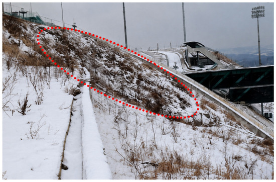
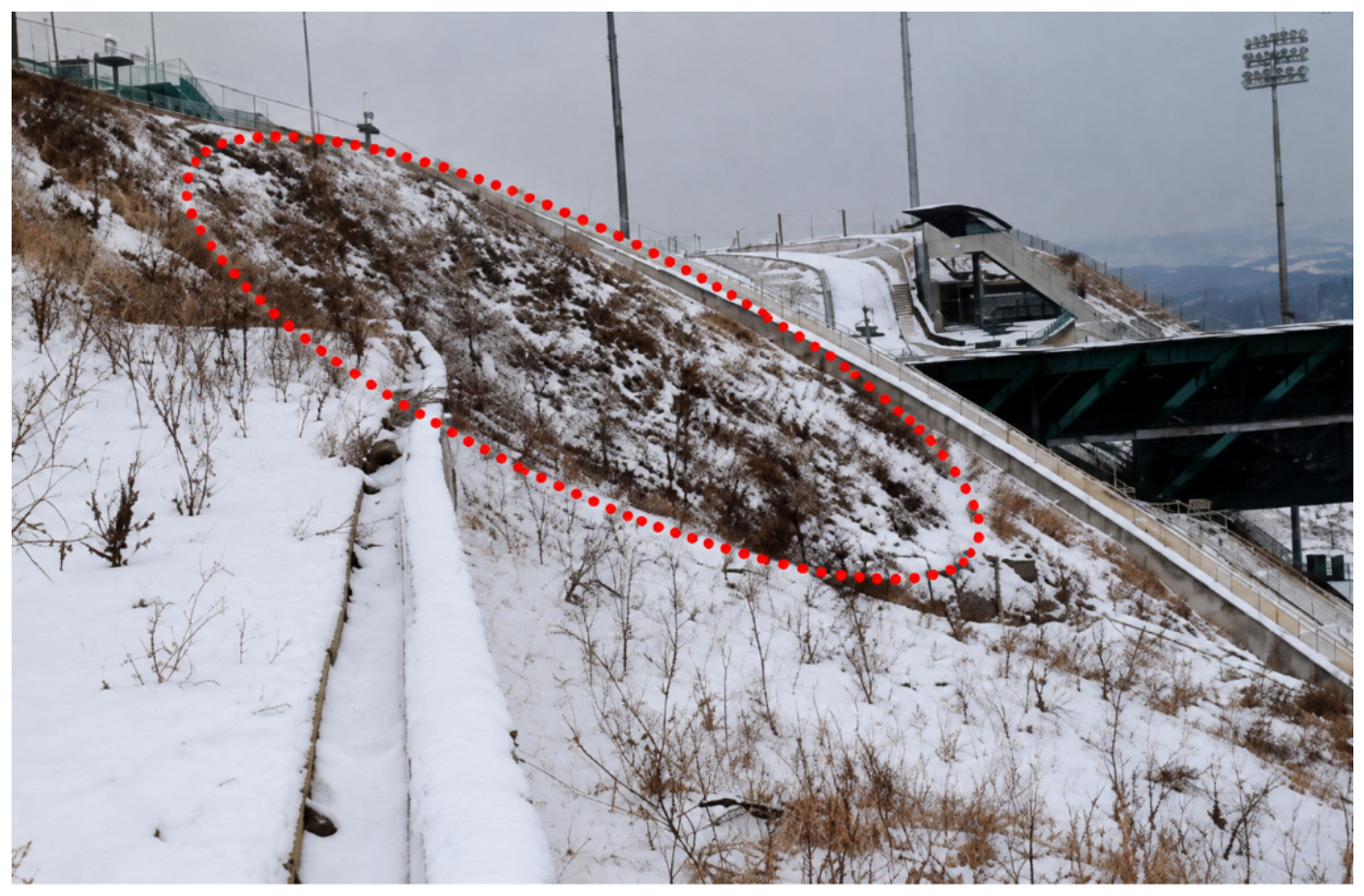
The slope under consideration is located in Alatau mountains and is shown in Figure 1.

Figure 1. General view of slope. The red dashed outline marks the extent of the landslide body identified during the site inspection.

In addition, all of the approaches described above share a common and significant limitation: they do not account for the progressive development of the collapse surface. Because of the inhomogeneity of the stress state, the limit-equilibrium condition is first satisfied at a single point within the soil massif; the collapse region then grows, and once it reaches the ground surface, the slope fails. Neglecting this progressive mechanism is not conservative with respect to the slope stability margin and therefore requires more careful consideration. Furthermore, when these methods are applied to reinforced soil massifs, they fail to account for the influence of the reinforcing elements themselves on the stress–strain state of the massif.

To address these limitations, the present study formulates and solves two related limit-equilibrium problems:

(1)

Analysis of the limit equilibrium of a heterogeneous soil massif, accounting for the progressive development of the collapse surface.

(2)

Analysis of the limit equilibrium of a heterogeneous soil mass, in which heterogeneity is artificially created by securing it with retaining walls. The heterogeneity of the massif arises from geological features (subsidence soil and from its artificial reinforcement by retaining walls).

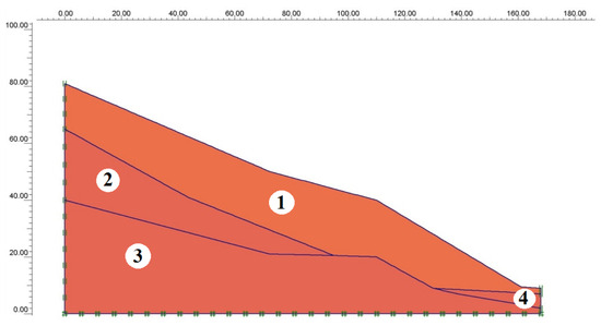
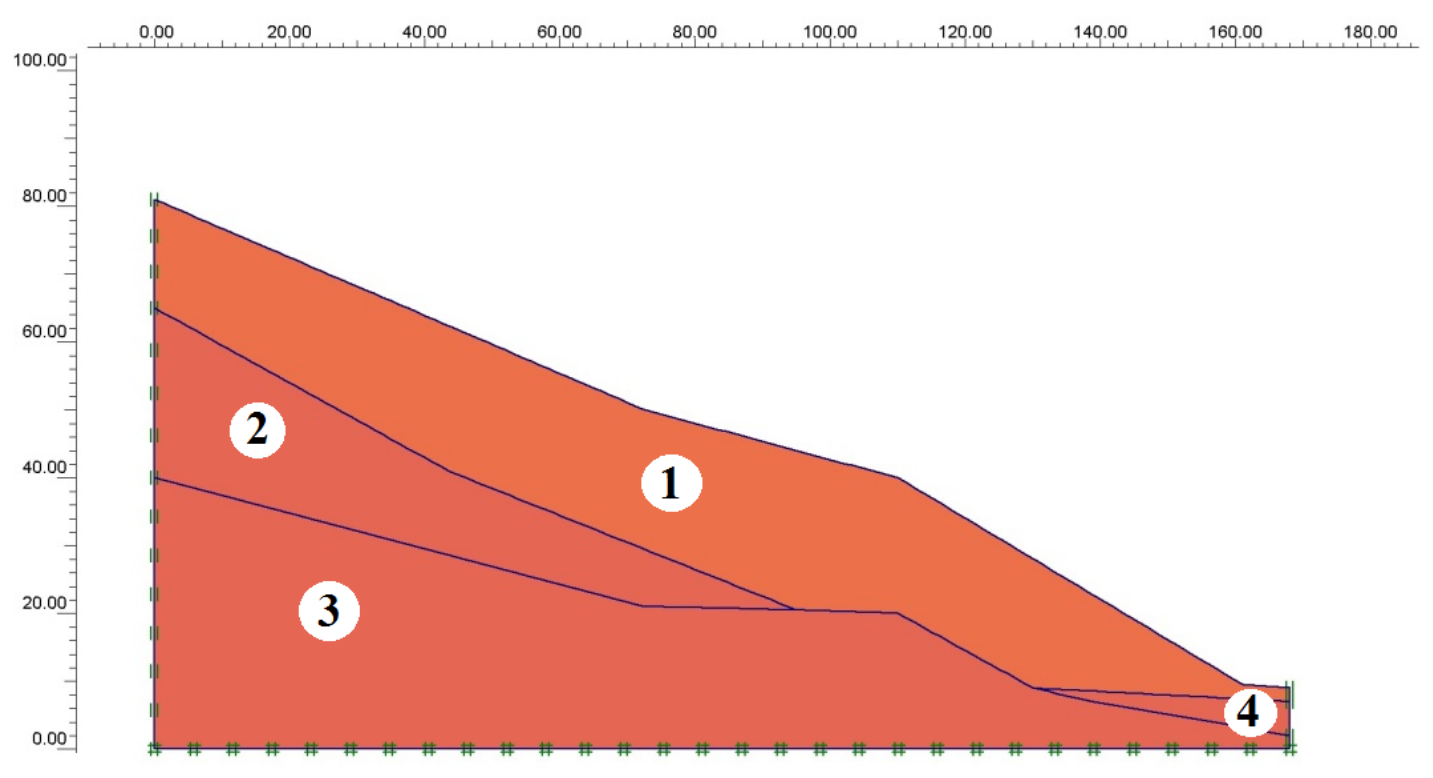
The second problem is illustrated by the case shown in Figure 2, in which the subsidence-prone slope is reinforced with a concrete retaining wall. The base of the concrete retaining wall is founded on solid loam bedrock (layer 3). The retaining wall is designed to prevent potential slope sliding caused by the subsidence soils.

Figure 2. Cross-section of the natural massif of the slope. 1—This region is represented by subsidence clays up to 30.0 m thick, subject to subsidence when moistened; 2—The area composed of loams, not subsidence, solid; 3—The area composed of rocks (treated as an effectively rigid base in the geometric model of Figure 2; represented in the finite-element calculation of Section 3 by the pebble/gravel soil layer, see Table 1); 4—The region made up of gravel soils with impurities in the plant layer.

The slope area is thus divided into several subregions corresponding to different soil characteristics (Figure 2). Different constitutive relations apply in each subregion. In subregions 1–4, the constitutive relations of soil mechanics are used with a prescribed pressure (from self-weight) and an initial porosity coefficient e ≥ 1. In the subsidence subregion, the same relations apply, but the initial soil pressure is obtained from the self-weight solution of the problem. Within the part of subregion 1 reinforced by the retaining wall, the relations of the theory of elasticity for reinforced soils are used.

The mathematical formulation of the problem follows established approaches, and the limit-equilibrium problem is solved using a geometrically linear formulation. However, this formulation excludes the possibility of studying local buckling (deformation localization), which can significantly affect the subsequent behavior of the soil mass.

We now formulate possible solution strategies for the limit-equilibrium problem. The traditional approach is based on solving a geometrically linear problem supplemented by a limit-equilibrium condition; the Coulomb–Mohr and Schleicher–Mises conditions are commonly used for this purpose. The two conditions differ only slightly, but the latter is more convenient in practice. Since the constitutive relations of plasticity theory are usually formulated in terms of velocities, the stress state must be determined during loading, and the limit-equilibrium condition must be checked at each point of the slope. If this condition is satisfied along a line that reaches the ground surface, the slope is considered unstable.

The soil mass was modelled as three layers—subsidence loams, non-subsidence loams and pebble/gravel soils—whose deformation and strength characteristics, adopted in the finite element calculations, are given in Table 1.

Table 1. Characteristics of soils adopted in the calculations of the FEM.

Layer Name	E, MPa	ν	γ, kN/m3	ϕ, deg	e0	λ	k
Drawdown loams	5.0	0.40	16.5	26	0.60	0.312	0.100
Non-subsidence loams	19.2	0.40	17.9	18	0.60	0.312	0.100
Pebble/gravel soils	68.0	0.40	21.1	35	0.60	0.312	0.100

Table 1. Characteristics of soils adopted in the calculations of the FEM.

Layer Name	E, MPa	ν	γ, kN/m3	ϕ, deg	e0	λ	k
Drawdown loams	5.0	0.40	16.5	26	0.60	0.312	0.100
Non-subsidence loams	19.2	0.40	17.9	18	0.60	0.312	0.100
Pebble/gravel soils	68.0	0.40	21.1	35	0.60	0.312	0.100

Analysis of the constitutive relations used in soil mechanics shows that the limit-equilibrium condition is inherently embedded in these theories, manifesting as exhaustion of the soil’s bearing capacity. The loading curve reaches a maximum, beyond which so-called “limiting” behavior begins: the soil stiffness decreases sharply, and localization of plastic deformation becomes possible. In this case, the limit-equilibrium problem reduces to a problem of stability and post-critical behavior of an inhomogeneous soil mass.

Collapse is analyzed directly by solving the plasticity problem together with the limiting conditions. Since only small strains are considered, the Cauchy stress-rate tensor is used as the measure of stress, and the small strain-rate tensor as the measure of strain. The stress–strain state is obtained by solving the following system of equations:

The equilibrium equation:

$$\nabla \mathrm{x}\mathsf{\sigma }+\mathrm{F}=0,\forall t\in (0,\mathrm{\infty });$$

(1)

The kinematic relation:

$$\mathsf{έ}=\raisebox{1ex}{$1$}\!\left/ \!\raisebox{-1ex}{$2$}\right.\left(\right);\nabla \mathsf{\nu }+\nabla \mathsf{\nu }$$

(2)

The constitutive relation:

σ = D:έ;

(3)

And the boundary conditions:

Nσ = T, on S_t and ν = ν₀, on S_u;

(4)

Here, σ is the Cauchy stress-rate tensor and F is the body-force vector in Equation (1); έ is the small strain-rate tensor and v is the velocity vector in Equation (2); D is the tensor of elastic moduli relating stress and strain rates in Equation (3); and in the boundary conditions of Equation (4), N is the outward unit normal, T is the prescribed traction on the traction boundary S_t, and v = v₀ is the prescribed velocity on the displacement boundary S_u.

Thus, to analyze the limit equilibrium, the plasticity problem (1)–(4) is solved and the limit-equilibrium condition is checked while accounting for the mechanical behavior of the subsiding soils. Following [28], the strength of a soil massif is estimated from the distribution of the stability coefficient η, calculated at different points of the slope. The coefficient η is determined by the formula:

η = σ_α^pr/σ_α,

(5)

where σ_α is the shear stress acting on the most critical planes, inclined at an angle –α to the principal planes; σ_α^pr is the shear stress at which the state of limit equilibrium is reached on these planes.

The limiting state on the shear planes is characterized by the Mohr–Coulomb condition:

σ_α^pr − σ_ntgφ − C = 0.

(6)

Here σ_n is the normal stress acting on the shear plane, φ is the angle of internal friction, and C is the cohesion of the given soil.

Shear planes are those inclined to the principal axes at an angle

α = (π/4 + φ/2)

(7)

Then we obtain the following expression for the stability coefficient:

η = (σ₁ + σ₂ + 2C ctg φ) sin φ/(σ₁ − σ₂)sin φ − tg φ,

(8)

For η < 1, the slope soils retain a margin of stability; at η = 1 the state of limit equilibrium is reached; and for η > 1, the strength of the slope soils is exceeded. Calculating the stability coefficient throughout the domain makes it possible to identify the zones of instability (η > 1). Where the limit-equilibrium condition is satisfied along a continuous line reaching the ground surface, the slope is considered unstable, and this line defines the extent of the collapse region. We now consider the case in which part of the region soil mass is reinforced with an elastic inclusion, namely a reinforced-concrete retaining wall. When the volume fraction of the inclusion is small, this problem reduces to the limit-equilibrium problem for the slope. The retaining wall itself can act as a source of stress concentration and thus cause local failure; however, from the standpoint of the overall stability of the slope, it is the average properties of the soil–wall system that matter, which allows the discrete heterogeneity to be treated as an equivalent continuous heterogeneity. This approach makes it possible to formulate the problem of controlling the stiffness distribution of the soil mass by means of retaining walls. In what follows, it is assumed that the retaining wall has a length comparable to the dimensions of the domain, that its axis is parallel to the slope, and that both the soil and the wall behave elastically. Associating the retaining wall with a local coordinate system, the constitutive relations of the transversally isotropic theory of elasticity (for the case of plane strain) take the form

σ₁₁ = C₁₁ε₁₁ + C₁₂ε₁₂

σ₂₂ = C₁₂ε₁₁ + C₂₂ε₂₂

(9)

σ₃₃ = C₁₂ε₁₁ + C₂₃ε₂₂

σ₁₂ = 2C₆₆ε₁₂

The five constants C₁₁, C₁₂, C₂₂, C₂₃, and C₆₆ denote five independent effective properties of the medium. They are expressed in terms of the technical constants K₁₁, K₂₃, μ₁₂, G₁₂, and G₂₃ as follows:

C₁₁ = E₁₁+ 4μ²₁₂C₆₆

C₁₂ = 2K₂₃μ₁₂

C₂₂ = G₂₃ + K₂₃

(10)

C₆₆ = G₁₂

C₂₃ = −G₂₃ + K₂₃

Here, E₁₁ is the elastic modulus under uniaxial loading, μ₁₂ is Poisson’s ratio characterizing the change in transverse dimensions under uniaxial loading, K₂₃ is the bulk modulus under plane strain, and G₁₂, G₂₃ are the shear moduli. The technical constants of the equivalent isotropic medium are obtained from the known mechanical characteristics of the soil, after which the limit-equilibrium problem for the slope reduces to solving the governing system for an inhomogeneous medium of prescribed geometry.

Within this framework, the problem of slope reinforcement can be formulated as follows: determine the orientation and the minimum volume fraction of the reinforcing elements such that the condition η > 1 is not satisfied anywhere in the domain, or is satisfied only within local zones of the soil massif. The finite element method is then used in a plane formulation, reducing the problem to constructing the stress field and subsequently identifying the line corresponding to a possible collapse surface. The location of the soil layers and their mechanical properties within the zone of increased load (due to increased moisture content) are assumed to be known, and the soil massif is treated under plane-strain conditions. A Cartesian coordinate system is associated with the half-space, with the 0 × 3 axis directed along the slope. The computational domain is taken as shown in Figure 2, with dimensions chosen so that the proximity of the boundaries does not introduce significant distortion into the stress–strain state within the zone of increased load; the specific domain size was established through computational experiments. On the boundaries x₁ = 0 and x₂ = 0, displacements are fully restrained. The rest of the boundary is assumed to be stress-free, except for the area of increased load from its own weight. Once the stress field for the slope is obtained, the condition η = 1 can be checked throughout the domain.

If a slip line forms that fully intersects the slope, or comes close to doing so, reinforcing elements (retaining walls) are installed on the slope. It is natural to reinforce the slope at locations where the stability coefficient is highest, placing the reinforcing elements perpendicular to the slip line. A control calculation is then performed, using the mechanical properties of the soil within the reinforced zones. If the results remain unsatisfactory, the reinforcement scheme is revised based on the new calculation and the problem is solved again. Compared with traditional slope-stability methods, the proposed approach allows slope stability to be assessed without preliminarily selecting a probable slip line—a task that is particularly difficult for a heterogeneous soil mass containing reinforcing elements.

When the material behavior is set to undrained, PLAXIS 7.2 automatically assigns an implicit undrained bulk modulus K to the entire soil (soil skeleton plus pore water) and distinguishes total stresses (undrained behavior):

∆p = K_ν∆ε_ν

(11)

The model parameters E_u, ν_u, c_u, and φ_u are entered in the soil dataset. The undrained bulk modulus is calculated automatically by the software using Hooke’s law:

K_ν =2G(1 + ν_ν)/3(1 − 2ν_ν)

(12)

G= E_u/2(1 + ν_ν) and ν^ν = 0.495

(13)

Here, Δp is the increment of pore pressure and Δε_v is the increment of volumetric strain in Equation (11); K_v is the undrained bulk modulus in Equations (12) and (13), G is the shear modulus, E_u is the undrained Young’s modulus, and ν_v is the undrained Poisson’s ratio, taken as 0.495 to approximate incompressible undrained behavior.

Tension cut-off: In this problem, regions of tensile stress may develop. According to the Coulomb envelope, tensile stresses are admissible provided the shear stress (the radius of the Mohr circle) is sufficiently low. However, the clay soil surface near the retaining wall often develops tension cracks, indicating that the soil cannot sustain tensile stress. This behavior can be incorporated in the PLAXIS analysis using the Tension cut-off option, which excludes Mohr circles with positive principal stresses. Selecting the cut-off option allows the allowable tensile strength to be specified; for the Mohr–Coulomb model, the default tensile strength is zero.

Interface strength (Rinter): An elastic–plastic model is used to describe the behavior of the interface between the soil and the retaining wall. The Coulomb criterion distinguishes elastic interface behavior, involving small internal displacements, from plastic behavior (slippage).

In order for the interface to remain elastic, the shear stress is given by the following expression:

τ < σ_ntgφ + c_u

(14)

and for plastic behavior:

τ = σ_ntgφ + c_u

(15)

where φ and c_u are, respectively, the friction angle and interface cohesion.

The strength properties of the interfaces are related to those of the adjacent soil layer through a reduction factor assigned to each data set. The retaining wall was analyzed using the finite element method within the theory of limit states of a granular medium, implemented in the PLAXIS software. The stress–strain state of the slope during its interaction with the retaining wall was evaluated for subsidence soils. A plane-strain problem was formulated using the Coulomb–Prandtl elastic–plastic model, which assumes elastic behavior below the yield point and isochoric (zero-dilatancy) plastic flow at the yield point. The elastic–plastic solution was obtained by the finite element method using the well-known “initial stress” approach, based on the Newton–Raphson iterative procedure with a constant stiffness matrix and a variable load vector, updated at each iteration by the “initial forces” arising in the plastic elements. The error in the FEM calculation comprised the discretization error, resulting from the replacement of a continuum with infinitely many degrees of freedom by a model with a finite number of degrees of freedom, and the round-off error arising from numerical computation.

3. Results

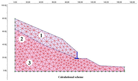
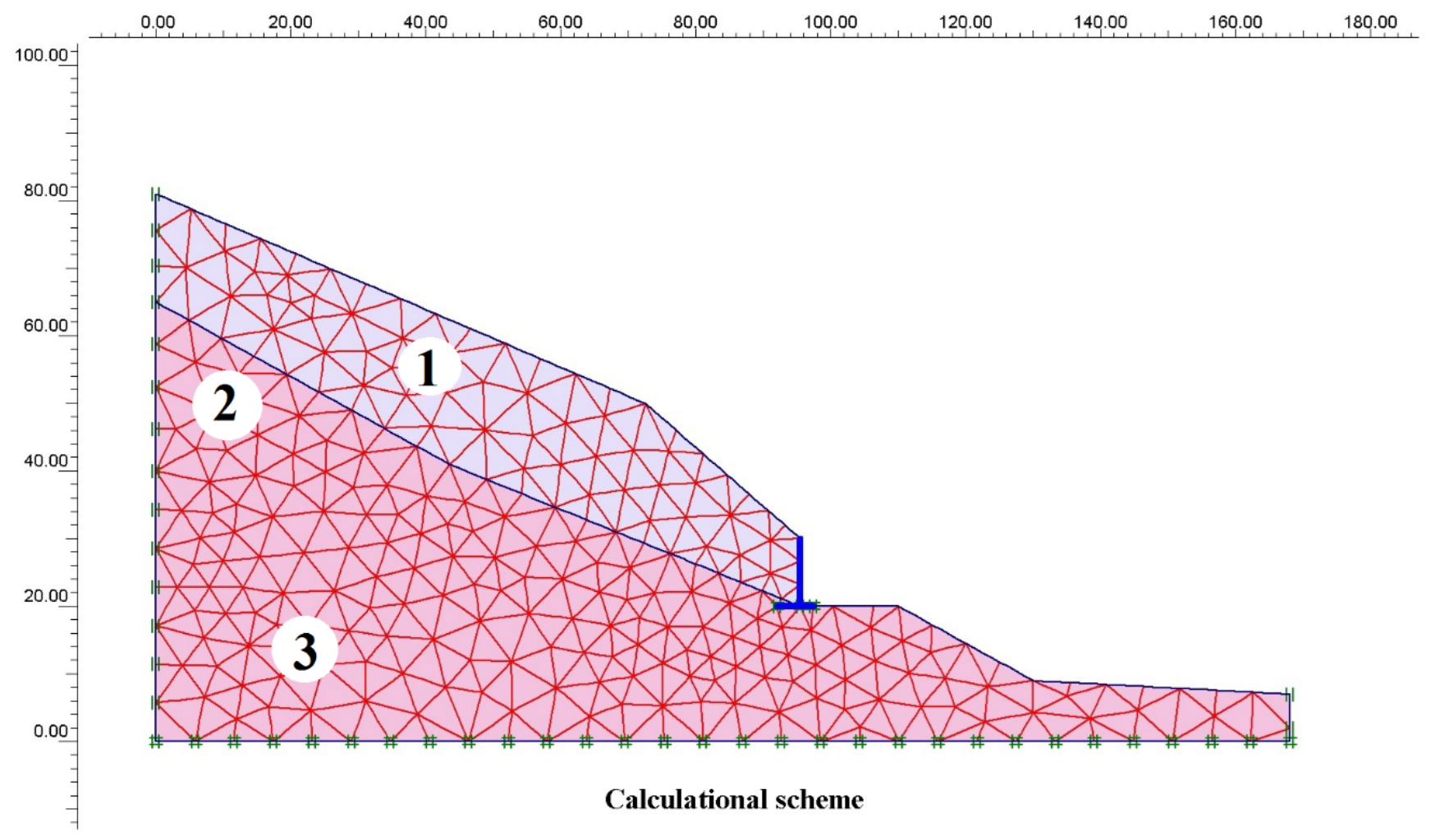
The stress–strain state of a slope composed of subsidence soils was studied for a moisture content increase from 15 to 30 percent of the initial value under the action of the soil’s self-weight (gravity). The calculation scheme, including the bedding layers, is shown in Figure 3: the first layer comprises subsidence soils up to 40 m thick, the second layer consists of hard, dense bedrock loams, and the third layer is pebble/gravel soil. The model therefore consists of three main soil layers. The problem was solved using the finite element method, with the Mohr–Coulomb model as the constitutive formulation. The physical parameters used in the calculation are given in Table 1.

Figure 3. Calculation scheme with a finite element mesh (1—subsidence loams; 2—non-subsidence loams; 3—pebble/gravel soils; see Table 1).

Figure 3 shows the calculation scheme together with the finite element mesh.

A slope with an inclination angle of 60° was considered, with the specific weight of the soil taken as γ = 16.5 kN/m³. Under this self-weight loading, a zone of plastic deformation and localization develops, shown in Figure 3 (layer 1). The slope state in this case can be described as close to the limit; nevertheless, the slope can be considered stable, since both zones reach the slope surface at only one edge.

The results of the solved plane problem are shown in Figure 4 and Figure 5.

Figure 4. Areas of localization of plastic horizontal movements.

Figure 5. Areas of localization of plastic shear stresses.

The numerical analysis yielded the following results:

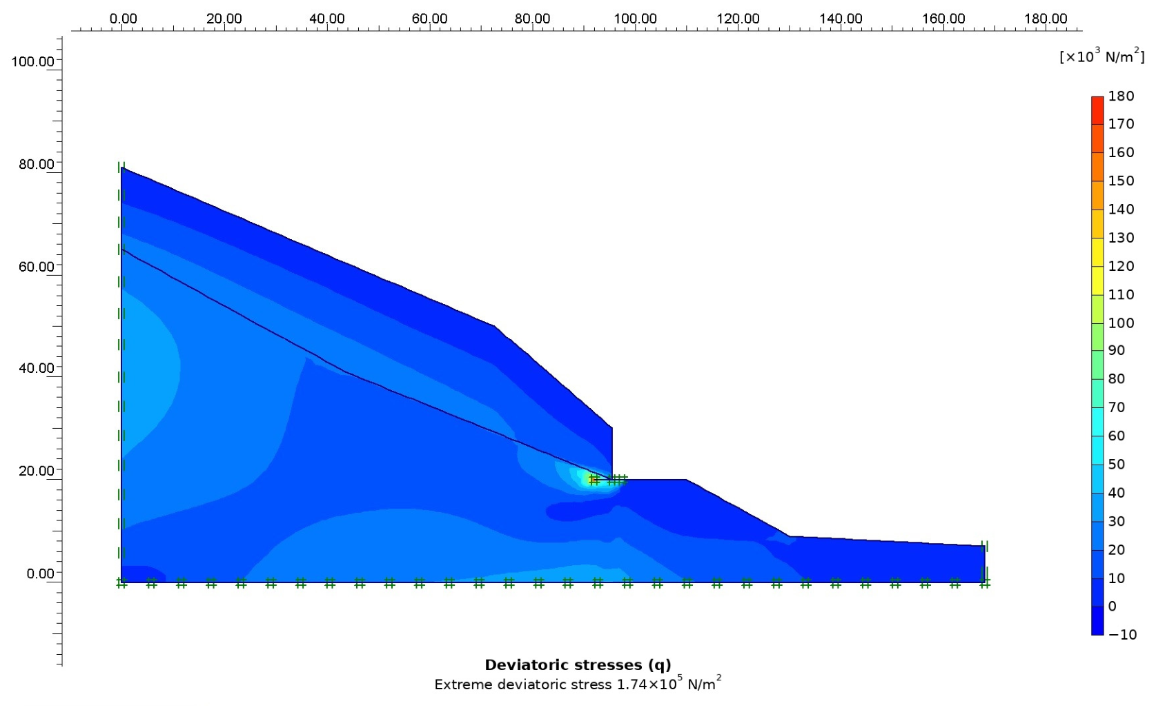
The development of horizontal and total displacements; the vertical total stresses; the development of plastic shear stresses; and the distortion of the finite element mesh following water saturation.

The stability factor is defined as the ratio of the specific weight at which the localization zone reaches the slope surface to the actual specific weight of the soil.

The numerical analysis further yielded the finite element mesh distortion, the horizontal and total slope deformations as the strength characteristics of the subsidence soils were varied, and the isolines of maximum horizontal (shear) stress and total stress for the slope-retaining wall interaction.

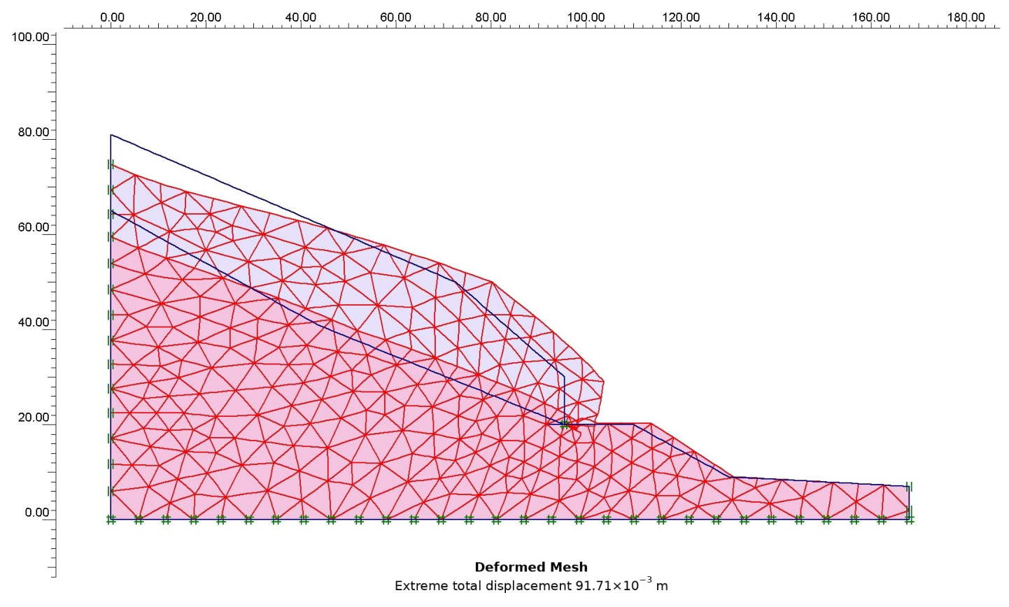
The corresponding distribution of total displacements and the deformed finite element mesh are shown in Figure 6.

Figure 6. Deformation mechanism (general displacements).

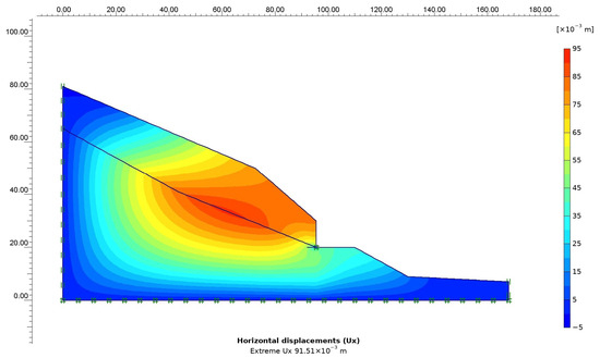
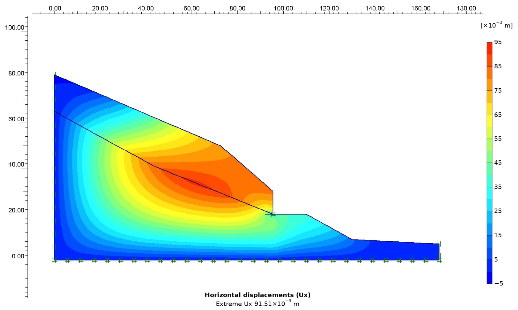
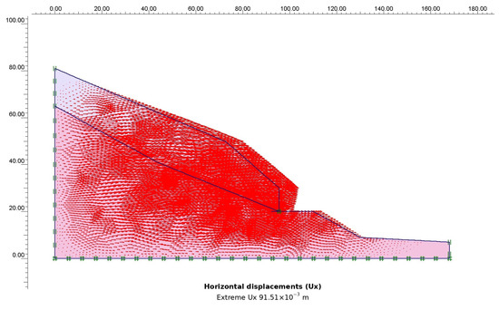
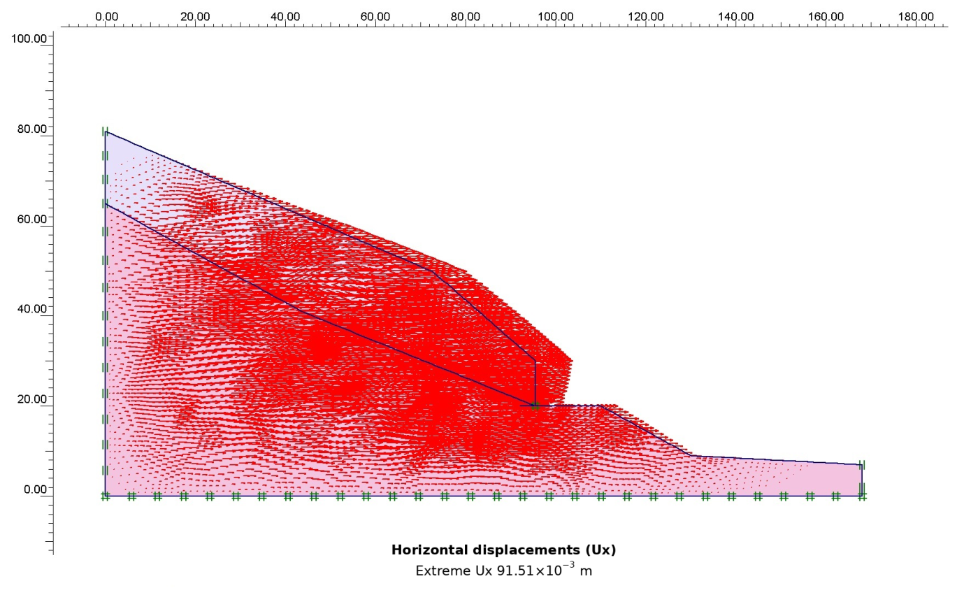
The distribution of horizontal displacements (U_x) within the slope is presented in Figure 7. The maximum horizontal displacement reaches 91.51 × 10⁻³ m.

Figure 7. Distribution of horizontal displacements in soil mass (Ux).

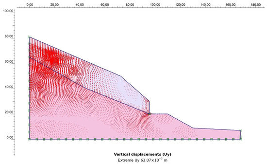
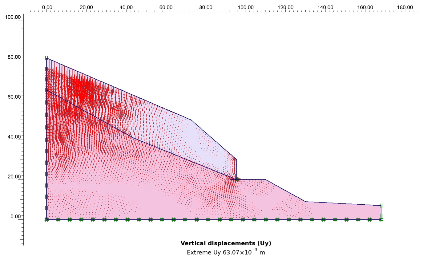
The distribution of vertical displacements (U_y) within the slope is shown in Figure 8. The maximum vertical displacement reaches 63.07 × 10⁻³ m.

Figure 8. Distribution of vertical displacements (Uy).

4. Discussion

The zone of local failure corresponds to a specific weight of γ = 16.5 kN/m³, for which the slope can be considered stable. As the additional mass load increases due to a 30% increase in moisture content, the zone of localized plastic deformation extends through the slope and reaches the ground surface from two sides; under these conditions, the slope becomes unstable and collapses.

Distributions of horizontal and total slope displacement were obtained for varying design characteristics of the subsidence soils, together with the isolines of maximum horizontal (shear) stress and total stress.

Analysis of the numerical results for the slope-retaining wall interaction shows that the most critical mechanism is the development of maximum horizontal deformation near the retaining walls, driven by shear. The zone of shear-deformation propagation extends through a large volume of the slope soils. Under self-weight loading and water saturation, the subsidence soils undergo settlement that reduces the initial cohesion, angle of internal friction, and deformation modulus, substantially altering the initial stress–strain state. The trajectories of soil particle movement during the slope-retaining wall interaction show that displacement is concentrated at the boundary between the subsidence and non-subsidence loams.

Novelty and relation to existing methods. The method presented here does not compete with general-purpose commercial finite-element codes such as PLAXIS, FLAC3D, GeoStudio, or RS2, all of which are capable of solving slope-retaining wall interaction problems within a Mohr–Coulomb framework. Its specific contribution is the explicit tracking of the progressive development of the collapse surface—obtained directly from the evolving stability-coefficient field η(x) (Equation (5)) rather than from a pre-selected slip-surface search—combined with a homogenization scheme (Equations (9) and (10)) that represents a discrete retaining wall as an equivalent continuous anisotropic inclusion for the purpose of limit-equilibrium analysis. This formulation could, in principle, be implemented within existing commercial codes; the present study should therefore be read as a proposed formulation and its finite-element implementation, rather than as a new standalone software tool.

Limitations. Several limitations of the present study should be noted. First, the numerical results reported here use the Mohr–Coulomb model exclusively; the reported advantages relative to a default PLAXIS Mohr–Coulomb setup do not necessarily extend to more advanced constitutive models such as Hardening Soil or Soft Soil, which capture stress-dependent stiffness and pre-consolidation effects not represented here. Second, the analysis is geometrically linear and does not address local buckling (deformation localization) or pore-pressure generation during undrained loading, both of which may influence the stress–strain state of soft, water-saturated subsidence soils. Third, the stability coefficient η obtained in this study has not been validated against field measurements, laboratory model tests, or independent numerical benchmarks; the two-phase comparison presented (slope without wall, then slope with wall) illustrates the method’s behavior but does not by itself constitute such a validation. Addressing these limitations—through quantitative benchmarking against commercial finite-element codes using more advanced constitutive models, and through comparison with field or laboratory data—is identified as the subject of a planned follow-up study.

Although the present study focuses on slope stability and retaining structures, the results obtained are directly relevant to the analysis of driven pile systems operating in heterogeneous, subsiding soils. The numerical framework developed here can be extended to assess the performance of pile foundations made of high-strength concrete, including those incorporating modified additives derived from industrial waste, by accounting for soil plasticity, stiffness redistribution, and progressive failure mechanisms.

5. Conclusions

Subsidence soils are widespread in the foothill regions of southern and eastern Kazakhstan, reaching thicknesses of up to 40 m. These soils undergo self-weight subsidence when wetted and exhibit pronounced dilatancy (liquefaction) and landslide susceptibility under water saturation.

The study addresses practical issues related to improving the efficiency of construction on subsidence soils. Since traditional experimental and theoretical methods proved insufficient for this purpose, new methodological tools were developed to solve this class of problems.

A method has been developed for calculating slope stability without predefining the shape of the collapse surface, using the equations of deformation mechanics for a weighty soil massif under different formulations of the limit-equilibrium condition. This study extends the traditional approach by explicitly incorporating the Coulomb–Mohr limit-equilibrium condition within the deformation theory of plasticity. The finite element method was adopted as the general numerical tool for obtaining the parameters that describe the behavior of the structure–soil system, allowing the mechanical inhomogeneity of the medium to be captured effectively and enabling calculation of the geometric changes in the domain that arise under large deformations.

Numerical analysis of the slope-retaining wall interaction shows that the most critical mechanism is the development of maximum horizontal displacements near the retaining walls, caused by shear deformation.

The developed numerical approach may be further applied to the analysis and modernization of driven pile foundations made of high-strength concrete, particularly when using modified additives derived from industrial waste, which is the subject of ongoing funded research.

References

- Cai, F.; Ugai, K. Numerical Analysis of Rainfall-Induced Landslides Considering Variations in Soil Hydraulic Properties. Eng. Geol. 2000, 55, 1–15. [Google Scholar]
- Bishop, A.W. The Use of the Slip Circle in the Stability Analysis of Slopes. Geotechnique 1955, 5, 7–17. [Google Scholar] [CrossRef] [Scilit]
- Li, P.; Vanapalli, S.K.; Li, T. Review of Collapse Triggering Mechanism of Collapsible Soils Due to Wetting. J. Rock Mech. Geotech. Eng. 2016, 8, 256–274. [Google Scholar] [CrossRef] [Scilit]
- Malyshev, M.V. Strength of Soils and Stability of Foundations of Structures; Stroyizdat: Moscow, Russia, 1994; 228p. (In Russian) [Google Scholar]
- Wei, L.; Zeng, Z.; Yan, J. Factors Affecting the Stability of Loess Landslides: A Review. Appl. Sci. 2024, 14, 2735. [Google Scholar] [CrossRef] [Scilit]
- Wei, G.; Yan, J.; Xia, Z.; Li, B.; Qi, H. Research on the Instability Mechanism of Loess Landslides Based on Preferential Infiltration of Rainfall. Front. Earth Sci. 2025, 13, 1586275. [Google Scholar] [CrossRef] [Scilit]
- Liu, X.; Zhang, Q.; Chen, H. Instability Mechanism of Loess–Mudstone Landslides under Rainfall Infiltration. Sci. Rep. 2025, 15, 1887. [Google Scholar] [CrossRef] [Scilit] [PubMed]
- Xiao, D.; Zhang, J.; Xu, W.; Wang, J.; Qiu, N.; Wu, J.; Ling, H.; Qu, B.; Yao, Z. Features of the Reinforcement–Soil Interfacial Effect in Fiber-Reinforced Soil Based on Pullout Tests. Constr. Mater. 2024, 4, 810–838. [Google Scholar] [CrossRef] [Scilit]
- Shakhmov, Z.A.; Zhussupbekov, A.Z. Frost Susceptibility of Soil and In-Situ Monitoring of Frost Depth in Construction. In Proceedings of the 15th Asian Regional Conference on Soil Mechanics and Geotechnical Engineering; ARC 2015: New Innovations and Sustainability; Taylor & Francis: Oxfordshire, UK, 2015. [Google Scholar] [CrossRef] [Scilit]
- Guo, P.; Zhao, W.; Qu, L.; Li, X.; Ma, Y.; Li, P. Review of Numerical Simulation of Overburden Grouting in Foundation Improvement. Geotechnics 2026, 6, 3. [Google Scholar] [CrossRef] [Scilit]
- Ukhov, S.B.; Semenov, V.V.; Znamenskii, V.V. Soil Mechanics, Bases and Foundations; Association of Engineering Institutions: Moscow, Russia, 1994. [Google Scholar]
- Morgenstern, N.R.; Price, V.E. A Numerical Method for Solving the Equations of Stability of General Slip Surfaces. Comput. J. 1967, 9, 388–393. [Google Scholar] [CrossRef] [Scilit]
- Terzaghi, K.; Peck, R.B.; Mesri, G. Soil Mechanics in Engineering Practice; John Wiley & Sons: Hoboken, NJ, USA, 1996. [Google Scholar]
- Fadeev, A.B. Finite Element Method in Geomechanics; Nedra: Moscow, Russia, 1987; 221p. [Google Scholar]
- Duncan, J.M. State of the Art: Limit Equilibrium and Finite-Element Analysis of Slopes. J. Geotech. Eng. 1996, 122, 577–596. [Google Scholar] [CrossRef] [Scilit]
- Phoon, K.K.; Kulhawy, F.H. Characterization of Geotechnical Variability. Can. Geotech. J. 1999, 36, 612–624. [Google Scholar] [CrossRef]
- Zhussupbekov, A.Z.; Utepov, Y.B.; Shakhmov, Z.A.; Ling, H.I. Model Testing of Piles in a Centrifuge for Prediction of Their In-Situ Performance. Soil Mech. Found. Eng. 2013, 50, 92–96. [Google Scholar] [CrossRef] [Scilit]
- Das, M. Braja Principles of Geotechnical Engineering, 3rd ed.; PWS Publishing Company: Boston, MA, USA, 1993; p. 67. [Google Scholar]
- Zhakulin, A.S. Deformability of Soils of Water-Saturated Bases; LAP Lambert Academic Publishing: Saarbrucken, Germany, 2015. [Google Scholar]
- Brinkgreve, R.; Broere, W.; Waterman, D. Plaxis 2D–Version 8; PLAXIS B.V.: Delft, The Netherlands, 2004. [Google Scholar]
- Huang, H.; Zhu, J.; Wu, Z.; Chen, J.; Tian, J. System Reliability Analysis of Slope Stability of Earth Rock Dams Based on Finite Element Strength Reduction Method. Appl. Sci. 2025, 15, 4672. [Google Scholar] [CrossRef] [Scilit]
- Yuan, W.; Zhang, W. Progressive Failure Mechanism of Sensitive Clay Slopes: Insights from Stabilized Smoothed Particle Finite Element Analysis of the 2010 Saint-Jude Landslide. Int. J. Numer. Anal. Methods Geomech. 2025, 49, 3251–3268. [Google Scholar] [CrossRef] [Scilit]
- Hu, C.; Zeng, Y.; Yao, H. Stability Analysis of Slopes with Cracks Using the Finite Element Limit Analysis Method. Front. Earth Sci. 2024, 12, 1364347. [Google Scholar] [CrossRef] [Scilit]
- Duan, Z.; Liu, Y.; Zhu, K.; Li, R.; Li, Y.; Yao, C. Loess Collapsibility Prediction and Influencing Factor Analysis Using Multiple Machine Learning Algorithms in Xi’an Region. Appl. Sci. 2025, 15, 12095. [Google Scholar] [CrossRef] [Scilit]
- Kacprzak, G.; Frydrych, M. Soil Consolidation Analysis in the Context of Intermediate Foundation as a New Material Perspective in the Calibration of Numerical–Material Models. Constr. Mater. 2023, 3, 414–433. [Google Scholar] [CrossRef] [Scilit]
- Xu, J.; Zhang, Y. AI-Powered Digital Twin Technology for Highway System Slope Stability Risk Monitoring. Geotechnics 2025, 5, 19. [Google Scholar] [CrossRef] [Scilit]
- Espinosa Fuentes, S.A.; El Naggar, M.H. Uncertainty Analysis and Quantification of Rainfall-Induced Slope Instability in Fine-Grained Clayey Soils. Geotechnics 2025, 5, 31. [Google Scholar] [CrossRef] [Scilit]
- Sellin, C.; Karstunen, M. Slope Stability Assessment in Sensitive Clay with an Advanced Constitutive Model. In Proceedings of the 10th European Conference on Numerical Methods in Geotechnical Engineering (NUMGE2023); Zdravković, L., Kontoe, S., Taborda, D.M.G., Tsiampousi, A., Eds.; ISSMGE: London, UK, 2023. [Google Scholar]
Disclaimer/Publisher’s Note: The statements, opinions and data contained in all publications are solely those of the individual author(s) and contributor(s) and not of MDPI and/or the editor(s). MDPI and/or the editor(s) disclaim responsibility for any injury to people or property resulting from any ideas, methods, instructions or products referred to in the content. |
© 2026 by the authors. Licensee MDPI, Basel, Switzerland. This article is an open access article distributed under the terms and conditions of the Creative Commons Attribution (CC BY) license.