


Abstract
Catastrophic disturbances pose significant challenges to remote sensing because landscapes can change rapidly, while access for field validation is limited, making it difficult to consistently track the spatiotemporal dynamics of discrete land-surface types. Building on the metaphor of the “ecosystem as an organism” and the individualistic perspective on ecosystems, each surface type is treated as a spectrally coherent entity whose identity must remain comparable over time despite changing conditions. To achieve this comparability, a Procrustes-based framework is introduced to align multi-index feature spaces from different dates to a common archetype, enabling cross-date classification within a commensurable coordinate system. Since Procrustes alignment requires a stable reference, the concept of core pixels (centroid-typical samples in feature space) is extended to spatially grounded anchor pixels that are invariant in both spectral and geographic space, thereby representing the persistent “organismal” structure of the landscape. Regression-based evaluation indicates that the Procrustes–anchor workflow improves classification fidelity and produces a clearer, more interpretable transition matrix of type changes, facilitating the separation of systematic transient dynamics from noisy reassignments. The resulting discrete habitat maps are independently validated using field geobotanical vegetation types, providing an ecological basis for the classified surface-type dynamics under catastrophic conditions.
1. Introduction
Assessing the spatial and temporal dynamics of terrestrial ecosystems from satellite remote sensing observations is a significant challenge with important practical and scientific implications [1,2]. Such dynamics can be represented either as continuous variation in environmental markers [3,4] or as temporal changes in the spatial configuration of qualitatively defined surface units, such as ecosystem types or structural landscape elements [5,6]. Spectral indices derived from satellite surface reflectance provide continuous proxies of environmental state, and their spatiotemporal variability is widely used to track ecosystem dynamics and infer ecological responses to environmental change [7,8]. Because vegetation is a key indicator of terrestrial ecosystem state and spatial heterogeneity, the Normalised Difference Vegetation Index (NDVI) remains one of the most widely used metrics for continuous monitoring of vegetation dynamics from satellite remote sensing data [9,10]. Beyond NDVI, a wide range of vegetation indices capture complementary aspects of plant functional status [11,12], such as canopy structure and high-biomass sensitivity (e.g., Enhanced Vegetation Index) [13], pigment and chlorophyll dynamics, including red-edge chlorophyll indices, photosynthetic light-use efficiency (e.g., Photochemical Reflectance Index) [14], and vegetation water status (e.g., water-related indices) [15]. A wide range of spectral indices also characterises the condition of soils, exposed substrates and rocks, as well as aquatic environments [16]. The radiometric and atmospheric-correction accuracy of satellite surface reflectance is a key determinant of how sensitively continuous spectral indicators can detect (and attribute) changes in ecosystem state, because surface-reflectance uncertainties propagate directly into downstream products such as vegetation indices [17]. When applying vegetation indices, particular care should be taken to minimise artefacts introduced by sensor differences, quality control, and compositing choices, as well as by atmospheric or sun–target–sensor geometry effects [8]. However, although continuous indicators quantify variation in biophysical properties, they do not, on their own, specify qualitative shifts among ecosystem or land-cover types, which require an explicit typology and categorical mapping framework [18]. The categorical mapping system has a fundamental advantage in discriminating between intratype variability and real transitions to another type [19], since individual spectral indices primarily record a combined quantitative signal rather than discrete qualitative states of Earth coverage, and change vectors based on indices describe the dynamics of change but do not provide clear evidence of qualitative transformations [20,21]. Ecological processes often depend on the shape and relative arrangement of discrete cover elements, such as fragmentation, edge effects, isolation, and connectivity, which are directly quantified using categorical maps [22,23]. In this framework, dynamics can be represented more informatively as transitions among classes using transition matrices or conversion typologies [24,25]. Many applied tasks, from biodiversity assessment to climate reporting, require stable categorical units over time to avoid spurious class changes caused by methodological updates or differences in input data [26,27,28]. This is particularly critical in rapid, catastrophic dynamics, where indices may fluctuate due to atmospheric effects, viewing geometry, bidirectional reflectance distribution function (BRDF) effects, and related artefacts. In contrast, categorical mapping combined with consistency control allows one to test whether apparent changes reflect structural transitions rather than noise [29,30].
Qualitative ecosystem specificity can be operationalised through ecosystem or land-cover typologies that represent the Earth’s surface as a mosaic of discrete units, enabling consistent mapping and temporal change analysis [6,31]. Notably, ecological theory has long contrasted two major views of ecosystems and communities: the Clementsian organismic (community-unit or complex superorganisms) paradigm that treats ecosystems as integrated entities [32], and the Gleasonian individualistic or continuum paradigm that views community patterns as the aggregate outcome of species-specific responses along environmental gradients [33]. The continuum paradigm treats an ecosystem as a mechanical assemblage of species, each exhibiting specific response patterns to environmental drivers [34]. Within this view, an “ecosystem” as a distinct entity emerges primarily from expert convention and consensus rather than from intrinsic system properties. Within the continuum paradigm, the apparent sharp ecosystem boundaries are interpreted as consequences of abrupt environmental gradients [35,36,37]. In this sense, the ecosystem concept is often regarded as an overstatement in the strict continuum paradigm, because the co-occurrence of species constitutes not a system per se but a contingent aggregate [38,39]. Yet Tansley—who coined the term “ecosystem”—criticised the Clements–Phillips organismal theory of vegetation and explicitly distinguished internally driven (autogenic) from externally driven (allogenic) succession, cautioning against treating vegetation units as organism-like entities [40,41]. Continuum gradient mapping was demonstrated to conserve the information in the floristic data best and does not require an a priori categorisation [42]. In this context, assessing ecosystem dynamics using continuous spectral indices is conceptually aligned with the continuum paradigm.
Organismic community paradigm, in contrast, treats an ecosystem as a genuine system: an assemblage of organisms that forms an integrated, coherent whole [43]. Although environmental conditions influence ecosystem boundaries, they are assumed to be determined primarily by internal, system-forming interactions [44]. Under this view, ecosystem types are real categories corresponding to qualitatively distinct entities in nature [45,46]. Communities that exhibit abrupt spatial changes might also be expected to show abrupt temporal changes as environmental conditions change gradually [43]. From an organism-like community paradigm, continuous spectral indices alone are insufficient to characterise ecosystem dynamics when ecosystems are treated as integrated units [47,48]. The continuous spectral index can be used to classify ecosystems or land-cover types [40,41,42]; however, this raises issues that extend beyond the technical accuracy of spectral measurements. In particular, classification requires a coherent definition of typological categories in spectral terms [49], and the ability to distinguish genuine spatial and temporal dynamics of types from spurious changes caused by classification errors or technical artefacts [50,51,52]. Thus, classification-based approaches become more complex. In addition to measurement accuracy, it is necessary to identify the qualitative invariance of ecosystems or land types under conditions of both quantitative variability in environmental parameters and conditions [53], as well as the properties of these discrete objects themselves [50,54].
Classification approaches can be broadly divided into supervised and unsupervised methods [55]. Supervised classification constitutes an explicit, hypothesis-driven inquiry in which mathematical decision rules are developed to distinguish predefined classes based on their spectral properties [56,57]. Its advantage is straightforward: objects delineated using ecological criteria can then be mapped and discriminated in feature space [58,59]. However, supervised approaches also entail systematic limitations. They implicitly assume that all relevant objects have been identified a priori [60,61] and that the resulting categories are spectrally homogeneous [62] and mutually separable based on spectral information [63]. This assumption is often reasonable for relatively stationary, quasi-climax, or late-successional communities, whose diagnostic composition is comparatively well characterised and whose rates of compositional change are low at the spatial and temporal scales relevant to mapping [64]. Template-based inference may fail under conditions of rapid spatial and temporal ecosystem dynamics, especially following catastrophic environmental disturbances. In such contexts, surface types may emerge and disappear quickly and may not fit established reference-class concepts [65,66]. Remote sensing may then become not a later stage of investigation but the starting point—sometimes the only means by which the existence of these objects can be detected. Under these circumstances, it is crucial not to dismiss novel patterns as classification artefacts, but to recognise them as potentially distinct land-surface or ecosystem types. This makes unsupervised classification, which does not assume predefined types, particularly relevant in highly dynamic environments.
The accuracy and ecological adequacy of unsupervised classification of remote sensing data depend on the observable spectral heterogeneity of Earth’s surface [67,68]. In turn, this heterogeneity depends on how sensitive spectral metrics are to the diversity of environmental conditions and ecological processes operating across landscapes [69]. A straightforward approach to robustly discriminate observed ecosystem types is to apply a sufficiently broad set of spectral indices that capture vegetation density and physiological status [8], moisture, and soil properties, including texture [70], mineralogical composition, organic matter, and salinity [71,72,73]. However, a purely mechanical increase in the number of spectral indices does not guarantee comprehensive coverage of all relevant ecological processes, because remote-sensing signals naturally integrate and mix information through canopy layering, interception and multiple scattering of radiation, and the combined contributions of numerous cover components [74]. Consequently, a key methodological challenge in unsupervised classification is to determine the effective number of meaningful cluster objects using procedures that enhance the information contributed by spectral components that are otherwise suppressed by more dominant sources of spectral variability.
Assessing the temporal dynamics of land-cover types raises the question of correspondence among classification units over time: to what extent are surface types comparable across time points, and are observed discrepancies driven by real ecological processes or by noise and systematic image artefacts? Conceptually, natural objects are assumed to retain their qualitative identity despite some degree of quantitative variability in their attributes. Detecting this identity in imagery requires that objects exhibit spectral specificity. A common way to represent such specificity is through phenological trajectories of spectral indices—typically vegetation indices and, very often, NDVI alone [64]. The temporal trajectory of an index can form a unique “fingerprint” that identifies an ecosystem type [75]. This approach is appropriate when, across the phenological window, the ecosystem maintains qualitative identity and spatial integrity. However, this requirement is often violated in ecosystems with pronounced spatiotemporal variability, particularly after catastrophic disturbances. In such settings, diagnostic information may reside less in temporal trajectories and more in the structure of the spectral feature space. The problem, therefore, shifts to amplifying underutilised (“hidden”) spectral dimensions to improve discrimination among land-cover types under rapid change.
Assessing land-surface type dynamics under rapid (especially catastrophic) change remains a non-trivial challenge. Building on an organism-like view of ecosystems and an individualistic perspective on community organization, this study applies the following workflow: (1) perform hierarchical, unsupervised spectral classification for each date; (2) determine the number of surface types from the observed spectral heterogeneity/homogeneity of the landscape; (3) estimate a Procrustean transformation between dates using spatially and spectrally invariant “anchor” pixels that operationalize a stable archetype for rotation into a common reference; and (4) reclassify the land surface in the shared, post-Procrustes feature space to obtain temporally comparable assignments and a clearer transition structure that separates systematic transient dynamics from noisy re-labelling, with the resulting types independently verified against vegetation-based habitat classes.
2. Materials and Methods
2.1. Study Area
Khortytsia Island (Ukraine) was selected as a case study of a territory that has undergone catastrophic change. Fieldwork was conducted on Khortytsia Island during 2024–2025 (Figure 1). Khortytsia is the largest island on the Dnipro River, located near the city of Zaporizhzhia, downstream of the Dnipro Hydroelectric Power Station. Oriented northwest–southeast, the island is approximately 12 km long and 1.6–2.7 km wide, covering 2359 hectares before the destruction of the Kakhovka Dam. Khortytsia lies within the northern extent of the former Kakhovka Reservoir. Following the destruction of the Kakhovka Dam and the Kakhovka Hydroelectric Power Plant in an explosion on 6 June 2023, the reservoir level dropped sharply; water levels in the Dnipro River decreased by about 8 m, according to records from the Nikopol hydrological gauging station [76]. The disaster triggered a series of changes that affected water bodies, soil, and vegetation [77].
Figure 1.
Study area overview: Ukraine and the Dnipro River reservoir cascade showing the position of Khortytsia Island near Zaporizhzhia, with a 3D relief model and a DEM map of the island’s southern part.
2.2. Stages of Analysis
The workflow integrates two complementary perspectives: the Gleasonian paradigm motivates the use of spectral indices as continuous descriptors of environmental variation, whereas the Clementsian paradigm of the ecosystem as an organism motivates the delineation and temporal comparison of discrete land-surface types. The overall sequence of data processing, cluster solution construction, Procrustes alignment, and class transition assessment is shown in Figure 2.
Figure 2.
Workflow of the Sentinel-2–based analysis for assessing spatiotemporal variability of landscape cover types: spectral index computation, harmonisation of predictors, pooled-space clustering, selection of core and anchor pixels, Procrustes consensus alignment, transformation of annual stacks into the consensus space, final classification, and subsequent quantification and interpretation of change.
2.3. Spectral Indices
At this stage, the analysis follows the Gleasonian paradigm, in which spectral indices are treated as continuous descriptors of environmental variation rather than as discrete ecosystem entities. The cluster classification approach used in this study was based on spectral indices derived from Sentinel-2 imagery. Spectral indices were employed as generalised quantitative measures of vegetation condition and dynamics, enabling comparisons across different time periods using consistent metrics and monitoring changes in the spectral properties of plant and soil components. Specifically, comparing distinct periods using individual indices is a standard method for assessing vegetation cover dynamics, and the Normalised Difference Vegetation Index (NDVI) is a fundamental indicator of vegetation change. The formulas for the indices used, along with their ecological significance, are presented and discussed in the protocol titled “Methods for Assessing the Temporal Dynamics of Landscape Cover Based on Procrustean Analysis of Spectral Indices,” which serves as the reference for calculation procedures and interpretation [78]. The following indices were calculated: Aerosol Contrast Index (AC_Index) [79], Blue-Green Index (BIG2) [80], Green Leaf Index (GLI) [81], Green NDVI (GNDVI) [82], Land Surface Water Index (LSWI) [83], Modified NDWI (MNDW) [84], Normalized Burn Ratio Index (NBRI) [85], Normalized Difference Bareness Index (NDBaI) [86], Normalized Difference Chlorophyll-a (NDChla) [87], Normalized Difference Green Chlorophyll Index (NDGCI) [88], Normalized Difference Index (NDI) [89], Normalized Difference Infrared Index (NDII) [90], Normalized Difference Iron Oxide (NDIO) [91], Blue-normalized difference vegetation index (BNDVI) [92], Normalized Difference Red Edge Index (NDRE) [93], Normalized Difference Red-Edge Improved (NDREI) [93], Normalized Difference Tillage Index (NDTI) [94], Normalized Difference Total Suspended Matter Index (NDTSM) [95], Normalized Difference Vegetation Index (NDVI) [96], Normalized Difference Water Index 1 (NDWI1) [97], Normalized Difference Water Index 2 (NDWI2) [98], Red–Blue NDVI (RBNDVI) [89], Red Edge NDVI 1 (RedEdge_NDVI1) [99], Red Edge NDVI 2 (RedEdge_NDVI2) [99], Red Edge Difference Index (REDI) [100], Red Edge Normalized Difference Vegetation Index (RENDVI) [82], Rock Index (RI) [101], Structure Insensitive Pigment Index (SIPI) [102], Sentinel–2 Vegetation Salinity Index (SVSI) [103], Tasseled cap greenness, brightness, and wetness indexes (TCI GREEN, TCI BRIGHT, TCI WET) [104], Modified soil-adjusted vegetation index (MSAVI) [105,106], Chlorophyll green (ClGRN) [107], Visual atmospheric resistance index (VARI) [108], Modified triangular vegetation index (MTVI2) [109]. The spectral index formulas and their ecological interpretations are presented in Table S1. Spectral indices were calculated using Sentinel-2 L2A (MSI) data for 9 and 14 June 2024, and 8 and 13 August 2025.
2.4. Starting Clustering
This step corresponds to the Clementsian paradigm of the ecosystem as an organism, because the aim is no longer merely to describe continuous spectral variation, but to delineate discrete, internally coherent land-surface entities. The cluster analysis was conducted in two stages. First, clustering was performed using the first two principal components extracted from the spectral indices. Second, clustering was refined on the basis of secondary principal components derived from the residuals of regression models of the spectral indices on the primary principal components. Previous clustering attempts indicated that, when delineating clusters, the “greenness” and “moisture” metrics play a dominant role, whereas the other spectral indices contribute little to the clustering decisions. To make fuller use of the information contained in the spectral index, clustering was therefore performed in two stages. In the first stage, spectral-index datasets from two consecutive acquisition dates—separated by several days within the same year—or from comparable dates one year apart were paired and merged to run clustering and obtain cluster assignments under similar rules and with consistent cluster labels. The optimal number of clusters (k) was determined using the Calinski–Harabasz criterion [110], selecting the k value that maximised the CH index for hierarchical Ward clustering partitions in the space of the first two principal components of spectral-index variability (PC1–PC2).
In the second stage, after obtaining the primary clusters in the PC1–PC2 space, the dominant spectral gradients were removed by constructing a ‘cleaned’ feature space. For each spectral index, the component explained by PC1 and PC2 was subtracted, and the resulting residuals, which capture finer variability beyond the main gradients, were then analysed. Repeated PCA (rPCA) was performed on the residual matrix, and the number of residual components retained for subsequent calculations was selected using the ‘elbow’ criterion applied to the scree plot. Next, within-cluster heterogeneity of the primary clusters in the rPC space was quantified using distances to the centroid and dispersion metrics. A second round of clustering was then conducted only within the most heterogeneous clusters. A primary cluster was considered heterogeneous if, in rPC space, it exhibited elevated within-cluster variability—characterised by large point-to-centroid distances and high dispersion, quantified by the trace and determinant of the covariance matrix—that is, if it fell within the upper part of the distribution of an integral variability metric (quantile threshold). Only such clusters were subjected to further subclustering. For each ‘variable’ parent class, Ward’s hierarchical clustering was applied in rPC space, and the number of subclasses (k2) was selected by maximising the Calinski–Harabasz index. Subclasses were parameterised by their centroids in rPC space. The resulting refinement rule was then applied to raster data. For most pixels, the level-1 label was retained, whereas pixels belonging to selected heterogeneous classes were reassigned to the nearest subclass centroid in rPC space.
2.5. Core and Anchor Pixels
The identification of core and anchor pixels follows the Clementsian paradigm of the ecosystem as an organism, because these pixels are interpreted as the most stable and structurally representative part of each ecosystem body in spectral space. At the subsequent stage, the identification of core and anchor pixels was carried out. Core pixels are the most representative pixels within each cluster for a given year, selected as those with the minimum distance to their cluster centroid. In other words, they constitute the “heart” of the class—pixels that best represent the cluster and are least marginal. Anchor pixels are the spatially invariant pixels [105] within the core set; that is, pixels that consistently retain their typicality across space. Core pixels are regarded as carriers of the most stable component of the multidimensional structure, representing centroid-typical spectral-index states of the clusters. Consequently, their cross-year consensus is interpreted as an invariant scaffold that reconstructs the spectral–spatial archetype of the studied landscape. Procrustes alignment is then employed to reconcile year-specific configurations relative to this archetype. Anchor pixels provide the reference correspondences used to minimise differences in the geometry of feature space; the remaining discrepancies can subsequently be interpreted as changes relative to the archetype rather than shifts in scale or orientation of the multidimensional space. For the anchor pixels, a generalized Procrustes analysis was applied to two datasets from consecutive dates. Transformations—including rotation, reflection, scaling, and translation—were estimated to minimize the sum of squared distances between corresponding rows of the two matrices. Simultaneously, a consensus configuration was estimated as a shared reference across both years, representing the mean shape of the aligned structure. This consensus configuration was interpreted as the spectral–spatial archetype, formed by the most typical states that are also the most consistent across years. Alignment quality was assessed using root-mean-square deviations: the distance of each aligned matrix to the consensus and the interannual distance before and after alignment. This allowed us to quantify the proportion of between-year differences explained by geometric alignment versus residual variability in the reference pixels.
Finally, the Procrustes parameters estimated from the anchor pixels were applied to the full index stacks for each year to bring all observations into a common consensus feature space. Specifically, for each year, the corresponding set of transformation parameters was obtained by aligning the “anchor” matrices to the consensus. The transformation was then applied stepwise to the index vectors of all pixels in the scene. This process produced two transformed index stacks corresponding to consecutive dates, aligned in consensus coordinates. This alignment ensured the comparability of multidimensional spectral profiles across dates within a single reference frame.
After the index stacks from consecutive dates were transformed into a common consensus feature space, they were merged into a single pooled array. Joint clustering was then performed on the aligned data. In this approach, pooling the two years is no longer merely a mechanical method for obtaining “matching class IDs,” as in the previous stage. Instead, prior Procrustes alignment minimises inter-date differences attributable to the global geometry of the feature space. It ensures that the compared index vectors represent the same multidimensional relationships within a single coordinate system. Consequently, cluster centroids derived from the pooled dataset can be interpreted as shared spectral–spatial archetypes, and assigning cluster labels to each year within the aligned space renders cross-year comparisons of labels meaningful. Following the joint clustering of the pooled, aligned stacks, the final cluster centroids were estimated within the consensus feature space and constructed a nearest-centroid classification rule. For each pixel at each date, the Euclidean distances to all centroids were calculated and assigned the label of the cluster with the minimum distance. Consequently, both temporal snapshots were assigned cluster labels defined within the same coordinate system (the consensus space), enabling direct comparison of classes between dates.
The transition maps were generated by comparing the label of each pixel between two dates to analyse spatiotemporal dynamics. Pixels whose cluster membership remained unchanged were interpreted as stable states, whereas changes in labels were treated as transitions between spectral–spatial archetypes. Transition intensity was quantified as the proportion of pixels exhibiting a label change, and/or as transition frequencies between cluster pairs within a transition matrix. This approach enabled a quantitative comparison of configurational cover changes both between consecutive dates and across years within a single aligned feature space.
2.6. Procrustes Stretch/Contraction Evaluation
Within the Clementsian framework, this procedure evaluates how effectively the spectral configurations from different dates can be brought into correspondence with a shared archetypal organisation of discrete land-surface types. For a given pair of acquisition dates, the two matrices of matched observations were formed: (date 1) and (date 2), where rows correspond to the exact pixel locations (a random subset of pixels), and columns correspond to p-spectral indexes. The agreement before and after the Procrustes stretch/contraction was evaluated by applying the same preprocessing/alignment pipeline to obtain Xc and Yc. An orthogonal Procrustes model was fitted both for observed and post-processed cases using the vegan::procrustes function and computed the residual matrix . Overall correspondence is summarized by the Procrustes RMS residual:
where Rij is an entry of the residual matrix , n is the number of pixels (rows) in the subset; p is the number of spectral indices, and reported as for before and for after Procrustes stretch/contraction.
A null distribution by randomly permuting the rows of Y (and separately Yc) B times was generated to quantify the mismatch expected under broken pixel correspondences, re-fitting Procrustes each time, and recomputing RMS. The mean of this distribution is reported as and . Because preprocessing changes the marginal distribution and scale of the feature space, the corresponding row-permuted null level can differ between the raw and post-processed cases. Therefore, null levels were estimated separately for each case. The normalized mismatch ratios and where reported, which serve as a dimensionless measure of agreement relative to the “random-pairing” baseline conceptually similar to normalized Procrustes distances where the mean null distance is set to 1. Whether the normalized relationship improves after stretch/contraction by applying a permutation sign-flip test to the mean difference of per-pixel normalized residual magnitudes (after vs. before) was tested. In addition, the improvement in absolute per-pixel Procrustes residual magnitudes was tested via a sign-flip test for (after − before). p-values were computed from B random sign-flip replicates. In operational terms, Procrustes efficiency was quantified as the decrease in the normalized mismatch ratio, D = (RMSbefore/Null RMSbefore) − (RMSafter/Null RMSafter), where larger positive values indicate stronger improvement in cross-date alignment.
2.7. Regression Analysis of Transitions Between Cluster Classification Solutions
The correct pixel-to-pixel correspondence is ensured for each pair of consecutive classification maps by geometrically harmonizing the input layers. An observation table was constructed for each consecutive map pair by randomly sampling n pixels from the overlapping area where both years have non-zero and non-NA values. The cell ID was recorded for each sampled pixel, including the x and y coordinates, the class label in the first year, and the class label in the subsequent year. The target variable was defined as a binary transition indicator:
i.e., (C = 1) if the pixel’s class changed between two consecutive maps, and (C = 0) if it remained the same.
Model predictors included: a clustering-method factor (Traditional vs. Procrustes-enhanced clustering), spectral “distance to cluster centroids” (fd), geographic distance to the “core” of the pixel’s own cluster (dc), and a topographic control.
We combined pixels from the two approaches (Traditional and Procrustes-enhanced clustering) into a single dataset to test whether the baseline transition probability differs between the methods. In the GLM model series, this was implemented as the factor Method.
Spectral distance to cluster centroids (fd) was computed for each pixel as the Euclidean distance in spectral-index space to the centroid of the nearest cluster. Centroid coordinates were obtained as the mean index values across the “core” pixels of each cluster.
Geographic distance to the cluster core (dc) was computed for each pixel as the minimum Euclidean distance in coordinate space (x, y) to the nearest core pixel of the same class (as defined in the reference year). In the code, this was implemented by looping over classes and calculating the minimum distance to the corresponding set of core coordinates (core_xy).
Topographic control () was included by extracting elevation from a DEM at pixel coordinates and standardizing it . A quadratic term was additionally included to allow for nonlinear effects of elevation on pixel transitions.
Transition probability was modelled using a binomial GLM with a logit link:
Models were fitted as a sequence of nested specifications, adding blocks of predictors step by step to report the gain in explanatory power and improvements in goodness of fit across the hierarchy:
- M0: intercept-only: ;
- M1: add method: ;
- M2: add spectral distance ();
- M3: add geographic distance ();
- M4: add topography ;
- M5 (key model): add interactions method: and method: , i.e., method-specific slopes for the spectral and spatial metrics.
The incremental contribution of each step in the model hierarchy was evaluated using ΔAIC, explained deviance, and likelihood-ratio tests (LRT). The regression coefficients on the log-odds scale (GLM estimates) were reported for the final model (M5), their standard errors, z-statistics, and p-values; odds ratios ; and 95% confidence intervals for OR computed as . Local extrema of the elevation effect were obtained from the quadratic term by solving for the stationary point of the linear predictor with respect to standardized elevation: . Because elevation was z-standardized , extrema was back-transformed to metres as , where and are the mean and standard deviation of elevation in the dataset.
2.8. Identification of Land Cover Types and Their Interpretation in Terms of the EUNIS Habitat Classification
Each spectral cluster was interpreted as an ecologically meaningful land-cover type by combining the following: (i) its position in PCA space and index profiles; (ii) spatial context (Dnipro main channel versus littoral zone, inner floodplain waterbodies, floodplain versus upper bank positions); (iii) microtopography and relative elevation within the floodplain; (iv) substrate or soil type (sand, mud/silt, clay); and (v) field-based physiognomy. During field surveys, the vegetation physiognomy and structure—including forest, shrub, tall helophyte reedbeds, ephemeral pioneer communities, and bare surfaces—were recorded, along with wetness conditions, signs of disturbance (such as ruderalisation and invasive species), and the most typical plant communities or associations characterized by diagnostic species. Spectral clusters were translated into EUNIS habitat types through expert-based matching of the combined spectral, geomorphological, and floristic or physiognomic evidence against the official EUNIS hierarchical habitat descriptions provided by the European Environment Agency.
2.9. Contingency-Table Association Statistics
An independent vegetation classification derived using the Braun–Blanquet approach was used for verification of the clustering results [111,112]. Details of the geobotanical vegetation relevés and the classification procedure are provided in our protocol [113,114]. The primary vegetation datasets are available through GBIF [115]. A contingency table of vegetation type by land-surface type was constructed for each classification method to evaluate the agreement between an independent geobotanical vegetation typology (comprising 20 types) and land-surface types derived from clustering Sentinel imagery (water-surface classes were excluded). The degree of structured association was quantified using three complementary measures: Cramer’s V, normalised mutual information (NMI), and conditional entropy (H).
Cramer’s V is a dimensionless measure of association strength for contingency tables [116]. Its underlying quantity is the mean square contingency (also known as “inertia” in correspondence analysis), denoted . It is defined in terms of cell probabilities and their marginal sums :
Building on , Cramér’s V for an contingency table is defined as:
Higher values of indicate a stronger association between the variables.
Because the classical sample estimator can exhibit substantial positive bias in finite samples—especially for contingency tables larger than —we used a bias-corrected estimator [116]. First, the empirical was computed from the observed cell proportions :
Next, the non-negative bias-corrected quantity and the adjusted (“effective”) table dimensions were derived, which yield :
We used this (bias-corrected Cramér’s V) to compare the two clustering methods.
Normalized mutual information (NMI) is an information-theoretic measure of dependence between two categorical variables, normalized by their entropies [117]. NMI increases as the mutual predictability of the two classifications increases and also lies in . For categorical variables and , let , , and denote their empirical probabilities. The mutual information is then defined as:
Entropies:
Normalised mutual information (NMI):
This normalization yields values in the range : indicates no information-theoretic association, whereas corresponds (under ideal conditions) to perfect agreement.
Conditional entropy is the average remaining uncertainty about vegetation type given the land-surface type, i.e., a measure of how diffuse the correspondence is between land-surface classes (from classification) and vegetation types. Smaller values of indicate a more structured association and better predictability of vegetation from the estimated land-surface class. The conditional entropy was computed as [118]:
where denotes vegetation type and denotes land-surface type. Lower values of therefore imply less uncertainty in vegetation type given the land-surface class—i.e., a more structured relationship and improved predictability of vegetation from the land-surface classification [119].
Comparison of the two classification methods was carried out in a paired design. Each pixel had two land-surface type assignments—one from the Traditional method and one from the Procrustes-enhanced method—while having a single vegetation-type label. The observed difference computed for each statistic as:
where denotes the statistic being compared (Cramér’s , NMI, or ). The direction of improvement was defined as follows: for Cramér’s and NMI, improvement corresponds to , whereas for improvement corresponds to .
The null hypothesis was formulated as follows: the land-surface classification method does not affect the degree of structured association between vegetation type and land-surface type; therefore, for each pixel, the “Traditional” and “Procrustes” labels are exchangeable. A paired permutation (swap) test was used to test this hypothesis. In each permutation, the two method-specific labels were independently swapped for each pixel with probability 0.5 and then recomputed . This generated a null distribution of that preserves the data structure (the distribution of vegetation types and the paired design) while breaking only the systematic difference between methods.
A one-sided p-value was computed as the proportion of permutations in which was at least as extreme as the observed value in the direction of the alternative hypothesis (with a +1 correction to avoid zero p-values). For Cramér’s and NMI:
For , the one-sided p-value was computed as:
where is the number of permutations. Results were considered statistically significant at . In addition, the mean and standard deviation of the null distribution of (Null mean, Null SD) were reported as a summary of the “random alternative” baseline. All computations were performed in R using custom code.
2.10. Clustering Decision Reliability as a Measure of Landscape Corrosion
The reliability of the clustering decisions was assessed using dismo: evaluate() as a general procedure for evaluating a threshold-based model that distinguishes each cluster from the remainder of the data. Two vectors of values were constructed for each cluster: (i) similarity values for the anchor pixels of that cluster (the target set), and (ii) similarity values for all other pixels in the scene (the non-target/background set), including anchor pixels from other clusters. The evaluate() function then computed confusion matrices across a range of thresholds and the associated performance statistics—specifically True Positive Rate (TPR), True Negative Rate (TNR), and Area Under the ROC Curve (AUC)—for each cluster. Based on these results, a cluster-specific threshold was selected by maximising TPR+TNR, which was interpreted as a quantitative boundary for the confident assignment of pixels to the respective cluster. Pixels that did not fall within the confident classification zone of any of the N identified clusters were labelled as an N+1 cluster.
Within the Clementsian paradigm, which views the ecosystem as an organism, these zones of unreliable clustering were interpreted as areas of landscape corrosion—that is, regions where the spectral–spatial integrity of the ecosystem is weakened and cluster membership cannot be assigned with sufficient confidence. In this context, landscape corrosion was operationally quantified by the occurrence and spatial extent of pixels assigned to the N+1 “uncertain” class. Thus, in the present study, unreliable clustering was treated not merely as a technical classification error but as an indicator of reduced internal integration of the ecosystem and, consequently, of ecological degradation. By contrast, within the Gleasonian paradigm, such misclassifications would be regarded primarily as technical classification problems rather than as evidence of impaired ecosystem integrity.
3. Results
3.1. Spectral Features of the Surface of the Studied Territory
First-order principal component analysis (PCA) demonstrated strong generalisation in explaining variability in the spectral indices. The first two components consistently accounted for the majority of the variance (approximately 84–89%; Table S2). The first principal component (PC1; 56–67%) represented a gradient of “greenness” and vegetation biomass, as evidenced by coherent loadings of vegetation indices such as NDVI, GNDVI, MSAVI, MTVI2, red-edge indices, and TCI_GREEN. The second principal component (PC2; 22–28%) described a moisture or wetness gradient, associated with differences in background brightness. It correlated systematically with water and moisture indices (NDWI2, MNDWI, TCI_WET, LSWI), alongside metrics sensitive to surface optical properties and soil background, notably TCI_BRIGHT, RI, and VARI. Therefore, for the floodplain area of Khortytsia Island, the principal spatiotemporal spectral contrast can be summarised as the balance between vegetation density and the hydrological regime.
Second-order PCA, conducted on residuals after removing the dominant first-order gradients, revealed variability that depends far less on vegetation quantity and much more on vegetation condition. The leading rPCs distinguished subtle differences in the physiological and pigment status of the vegetation cover, using red-edge and pigment-sensitive indices such as NDRE/NDREI, REDI, NDChla, and others, as well as soil surface characteristics (NDTI, NDBaI, TCI_BRIGHT, and related metrics). These parameters reflect the degree of exposure, texture, drying, or waterlogging of the substrate.
3.2. Cluster Solutions
Using paired images from 9 to 14 July 2024, the study area was clustered into 7 groups, whereas paired images from 8 to 13 August 2025 yielded 10 clusters (Figure S1A). Clustering based on images from different years, acquired at approximately comparable times, produced eleven clusters for July 2024 and 14 July 2025, and twelve clusters for 18 August 2024 and 13 August 2025 (Figure 3).
Figure 3.
Distribution of anchor pixels representing land-surface types identified by cluster analysis and projected onto the space of the first two primary (a,c) and the first two secondary (b,d) principal components ((a,b)—9 July 2024 and 14 July 2025; (c,d)—18 August 2024 and 13 August 2025). Type definitions: the numbering shown applies to the 18 August 2024 and 13 August 2025 images, and the numbering in parentheses applies to the 9 July 2024 and 14 July 2025 images: 1 (8, 11)—T13—Temperate hardwood riparian forest; 2 (4)—T11—Temperate Salix and Populus riparian forest; 3 (3)—C3.6—Unvegetated or sparsely vegetated shores with soft or mobile sediments; 4 (1)—Q51D2—Typha angustifolia beds normally without free-standing water; 5 (2)—E5.43—Shady woodland edge fringes; 6 (5)—C2.3—Permanent non-tidal, smooth-flowing watercourses; 7 (6)—Q511—Phragmites australis beds and F9.35—Riparian stands of invasive shrubs; 8 (10)—C3.53—Euro-Siberian annual river mud communities; 9 (7, 9)—Q61—Periodically exposed shore with stable, eutrophic sediments with pioneer or ephemeral vegetation; 10 (8, 11)—R11—Pannonian and Pontic sandy steppe; 11 (5)—C3.61—Unvegetated river sand banks; 12 (2)—C3.5132—Swards of small Cyperus species.
Thus, interannual clustering resulted in a greater number of clusters, and August-based clustering produced more clusters than July-based clustering. The first-order principal components (PC1 and PC2) were sufficient to separate the land surface into the majority of clusters, whereas the second-order PCA on residuals provided additional subclustering (Table 1). Clustering of consecutive-day image pairs yielded fewer primary clusters than interannual image pairs. The number of second-order PCs on residuals reflects additional information not captured by the primary spectral gradients, enabling subclustering of 2–4 primary clusters.
Table 1.
Summary of clustering and ordination outputs: number of primary clusters, number of second-order PCs on residuals retained, number of primary clusters selected for subclustering, number of subclusters, and total number of clusters.
Taken together, the patterns shown in Figure 3 and Figure S1, along with the quantitative results of the principal component analysis (Table S2), indicate that gradients in vegetation cover density and moisture are the principal factors governing the differentiation of land-cover types in the study area. The secondary principal component analysis further refines this differentiation by emphasising variables sensitive to the spectral characteristics of the soil surface and to indicators of plant functional status.
3.3. Procrustes Analysis
The core pixels were identified, based on the preceding clustering step, as those closest to the cluster centroids in spectral feature space within the initial dataset (2000 pixels per cluster). From this core set, anchor pixels were then selected—those that retained their membership in the corresponding cluster during the subsequent time period. The cross-date consensus of spectral indices for the anchor pixels forms a “spectral archetype” of land-surface types, assuming that this archetype remains invariant across both time and space. Therefore, a Procrustes “pull-to-consensus” transformation was derived from the anchor pixels and applied to all remaining pixels in the corresponding datasets. This procedure substantially improved the correspondence between the datasets (Table 2).
Table 2.
Assessment of Procrustes stretch/contraction efficiency for a pair of dates: RMS Procrustes residuals (RMS), null baseline (Null RMS), normalised ratios (RMS/Null RMS), and the sign-flip test for Δ.
3.4. Classification Transitions in Consecutive Images
Pixel-based classification outcomes vary between consecutive images. Intuitively, for images acquired only a few days apart, differences in classification results may arise from either random variation or systematic technical artefacts. For image pairs separated by one year, both relative stability of cluster assignments and genuine transitions can be expected—reflecting shifts in cluster boundaries driven by natural processes as well as technical errors and artefacts. Such changes can be summarised using transition matrices. Visual inspection of these matrices indicates that applying the Procrustes-based correspondence enhancement substantially reduces the number of pixel transitions over a few-day interval (Figure S2). A reduction in transitions was also observed for image pairs separated by 1 year (Figure 4), allowing comparison of transition patterns obtained with and without the Procrustes procedure. Particular attention should be paid to changes in the structure of the links and their relative strength. Together with the other diagnostic tests, this pattern may be used as additional evidence supporting the effectiveness of the Procrustes-based alignment.
Figure 4.
Transition-matrix visualization for the traditional method (a,c) and the Procrustes-improved method (b,d). Only transitions with probabilities >10% are shown ((a,b)—9 July 2024 and 14 July 2025; (c,d)—18 August 2024 and 13 August 2025).
Absolute RMS values after Procrustes stretch/contraction were markedly lower than those of the original datasets. The ratio of RMS to Null RMS was also significantly reduced following Procrustes stretch/contraction, indicating a genuine improvement in dataset alignment quality. Quantitatively, this is reflected in an increase in diagonal mass (the fraction of pixels remaining in the same class) and a corresponding decrease in off-diagonal mass (the fraction changing classes). For image pairs separated by a few days, Procrustes alignment increased diagonal mass from 37.49% to 49.07% for 9–14 July 2024 and from 52.72% to 80.02% for 8–13 August 2025 (Table 3).
Table 3.
Summary of transition-matrix and change-fragmentation metrics.
For pairs separated by one year, the effect was also retained: diagonal mass increased from 77.26% to 81.31% and from 43.26% to 53.82%, while the number of “changed pixels” decreased from 15,866 to 13,040 (−17.8%) and from 39,584 to 32,218 (−18.6%).
3.5. Factors Explaining Classification Transitions
Pixel transitions to other classification categories in images acquired only a few days apart are driven by systematic factors. Therefore, the hypothesis that such transitions are caused exclusively by random variation or technical artefacts can be rejected. The set of regular predictors (model M5) explained 4.42–8.11% of transition deviance for image pairs separated by a few days, and 1.29–5.90% for pairs separated by approximately one year (Table 4).
Table 4.
Sequential comparison of nested binomial GLMs (AIC and explained deviance).
In terms of importance, topography contributed the most significant incremental gain in explained deviance and the most substantial improvement in AIC, indicating that transition probability varies systematically along the elevation gradient in a nonlinear manner. The classification method also had a significant effect on transition odds, while the impact of spectral distance to class centroids and spatial distance to same-class core pixels were dependent on the method used, as evidenced by significant interaction terms. Procrustes enhancement was associated with a reduced likelihood of misclassification, as indicated by the negative regression coefficient for the Procrustes indicator (Table 5).
Table 5.
Model M5: estimated effects and odds ratios across survey periods.
The effects of elevation, as well as distances in spectral and geographic space, further support the presence of systematic drivers of transitions between cover types, driven by ecological processes and changes in cover configuration. Notably, such consistent drivers generate substantial dynamics even between images taken only a few days apart. Positive interaction coefficients between the Procrustes-enhanced method and distances in spectral and geographic space suggest that the method’s advantage increases in regions closer to the archetypal configuration. In other words, this approach provides exceptionally stable classifications for the most typical land-surface conditions. Within the 24–54 m elevation range, the quadratic elevation effect indicates a local minimum in pixel transition propensity at mid-low elevations (approximately 31.7–35.3 m). The only exception is the 9 July 2024 vs. 14 July 2025 pair, where the extremum reverses and corresponds to a local maximum at around 40.4 m.
3.6. Interpretation of Clusters Delineated from Surface Spectral Characteristics in Terms of EUNIS Habitat Types
Clusters delineated from the integrated spectral information (Figure 3 and Figure S1) and their spatial context within the floodplain–riverbank system (Figure 5 and Figure S3) were interpreted in terms of EUNIS habitat types (Table S4). In total, 12 ecologically meaningful habitat types were identified, spanning riparian forests (T13, T11), woodland-edge fringes (E5.43), flowing waters (C2.3), tall-helophyte stands (Q51D2, Q511), pioneer littoral communities on mud or sand and periodically exposed eutrophic sediments (C3.53, Q61), open sandy surfaces and psammophilous steppe (C3.6, C3.61, R11), and small Cyperus swards (C3.5132). However, the ability to discriminate among these types varied with the image-date window: for the August pairs (18 August 2024 and 13 August 2025) the full set of 12 classes was consistently resolved, whereas for the July pairs (9 Jul 2024 and 14 July 2025) several habitats converged or merged into shared clusters due to greater spectral similarity during that phenological period. The spatial pattern presented in Figure 5 also indicates a degree of conservatism and continuity in habitat types within the floodplain–riverbank system. A substantial proportion of habitat patches maintain their spatial position and overall configuration between dates, demonstrating the relative persistence of the main habitat structure. Nevertheless, transitions among habitat types are clearly evident. Unlike Figure 4, which details the structure and intensity of individual transitions, Figure 5 depicts all transitions using a single colour. This generalised representation is useful for identifying the principal spatial hotspots of transformation, which are concentrated primarily in the south-western and central parts of the island.
Figure 5.
Spatial variation in cluster distribution: the configuration for the initial period is shown on the right, whereas the configuration of pixels that retained their cluster assignment is shown on the left; pixels that changed their cluster assignment (the last pseudo-cluster) are as ‘13’ shown in black ((a,b)—9 July 2024 and 14 July 2025; (c,d)—18 August 2024 and 13 August 2025). Type definitions: the numbering shown applies to the 18 August 2024 and 13 August 2025 images, and the numbering in parentheses applies to the 9 July 2024 and 14 July 2025 images: 1 (8, 11)—T13—Temperate hardwood riparian forest; 2 (4)—T11—Temperate Salix and Populus riparian forest; 3 (3)—C3.6—Unvegetated or sparsely vegetated shores with soft or mobile sediments; 4 (1)—Q51D2—Typha angustifolia beds normally without free-standing water; 5 (2)—E5.43—Shady woodland edge fringes; 6 (5)—C2.3—Permanent non-tidal, smooth-flowing watercourses; 7 (6)—Q511—Phragmites australis beds and F9.35—Riparian stands of invasive shrubs; 8 (10)—C3.53—Euro-Siberian annual river mud communities; 9 (7, 9)—Q61—Periodically exposed shore with stable, eutrophic sediments with pioneer or ephemeral vegetation; 10 (8, 11)—R11—Pannonian and Pontic sandy steppe; 11 (5)—C3.61—Unvegetated river sand banks; 12 (2)—C3.5132—Swards of small Cyperus species.
3.7. Cross-Validation Using Geobotanical Relevés Indicates Clear Advantages of the Procrustes-Improved Clustering Procedure
The contingency tables linking vegetation community types to land-surface types show a measurable level of agreement between field-based classifications and classifications derived from spectral indices extracted from Sentinel imagery (Table S3). The Higher Cramer’s V and higher NMI, together with a lower conditional entropy H(Plant|Cover), indicate that the Procrustes-improved clustering yields a stronger and more structured correspondence with geobotanical vegetation types than the traditional clustering across all metrics (Table 6).
Table 6.
Comparison of contingency relationships between vegetation types (geobotanical classes) and Earth-surface classes derived from Sentinel imagery using the traditional clustering approach and the Procrustes-improved clustering procedure (N = 878 paired pixel–geobotanical plot records; α = 0.05).
The observed differences ( Procrustes − Traditional) were statistically significant relative to the null expectation under a paired swap permutation test (one-sided; ; ).
3.8. Zones of Unreliable Clustering: Landscape Corrosion Following the Disaster
Within the concept of the ecosystem as an organism, stable correlations among its structural and functional components are expected to maintain the integrity of its internal organization. Disturbance of these relationships should lead to deterioration in clustering quality, because weakening of intra-system integration is manifested as degradation, or corrosion, of the boundaries between such formations. Accordingly, zones of unreliable clustering can be interpreted as areas where the organism-like integrity of the ecosystem is most strongly disrupted. Zones of unreliable clustering exhibit a regular spatial pattern corresponding to areas severely affected by the catastrophic impact (Figure 6). In 2024, this zone primarily encompassed floodplain water bodies and the shoreline of the Dnipro River. By 2025, it had expanded to the eastern and south-eastern parts of the island, including both floodplain channels and relatively elevated sandy banks. The ongoing negative dynamics observed several years after the disaster can be aptly likened to landscape corrosion.
Figure 6.
Spatial variation in cluster distribution and areas of unreliable clustering. Pixels with unreliable clustering are shown in black, based on comparisons between 9 July 2024 and 14 July 2025: (a) 9 July 2024 and (b) 14 July 2025; and between 18 August 2024 and 13 August 2025: (c) 18 August 2024 and (d) 13 August 2025.
4. Discussion
4.1. From Spectral-Index Monitoring to Habitat Mapping After the Kakhovka Dam Collapse
The destruction of the Kakhovka dam triggered a surge of remote-sensing-based studies focused on documenting and analysing the consequences of this disaster [120,121,122]. This problem holds significant scientific, social, humanitarian, and economic importance. However, access to the area is severely restricted, as it remains an active combat zone, rendering remote sensing virtually the only viable method of investigation. Consequently, most studies to date have concentrated on the dynamics of spectral indices across the entire former reservoir area [123,124]. The combination of field geobotanical surveys and a Sentinel-based classification procedure made it possible to delineate the following habitat types across the entire reservoir area after the disaster: willow thickets, marshy vegetation, shells and sands, takyr-like substrates, and water bodies [125]. Our study focused on a local site that nonetheless includes habitat types representative of the entire reservoir, enabling us to describe the vegetation in detail and thus verify the mapped habitat classes. Addressing the challenge of tracking the spatiotemporal dynamics of discrete Earth-surface types under catastrophic conditions also prompted us to further develop the “ecosystem as an organism” concept as a logical framework for comparing satellite images over time.
4.2. Spectral Shape and Size of Ecosystem Bodies as Organisms
The metaphor of an ecosystem as an organism can also be productive in the context of procedures for identifying typological units of the Earth’s land cover from remote sensing data. The morphology of an organism is characterised by its size and shape [126]. Principal component analysis of the morphology of biological bodies typically yields the first one or two principal components that explain the overwhelming majority of variation in morphometric traits; these components capture variation in body size [127,128,129,130]. Body size reflects the extent to which a body occupies space. If the variation associated with the first principal components is removed from the original morphometric variables, a secondary principal component analysis will then produce variables that characterise body shape [131]. It is precisely shape that provides organisms with the qualitative specificity by which one distinguishes them [132]. Spectral indices may be interpreted as revealing the morphology of ecosystems-as-organisms in spectral space. Therefore, the size of ecosystems in spectral space is represented by the first two principal components of the variability of spectral indices, whereas the shape of ecosystems in spectral space is the variability represented by the second-order principal components on the residuals of spectral indices.
4.3. Recognition of Ecosystem Organisms: Clustering
The choice of a clustering procedure and the determination of the number of clusters constitute a fairly “creative” component of unsupervised classification [67]. An appropriate approach is to verify whether the procedure can recover spatial structures that are also detected by independent methods, i.e., to treat practical consistency as the ultimate test of validity. Ward’s method applied to Euclidean distances in the principal-component score space performed well. This is likely because the mathematical properties of the procedure are well aligned with the way ecosystem entities are structured in spectral space [133,134]. Ward’s method is therefore suitable for clustering spectral indices, as it minimizes within-cluster variance in Euclidean space and yields compact, well-separated groups, thereby improving the interpretability of the resulting land-cover types [135]. The optimal number of clusters should be determined primarily through expert judgement, while formal criteria play a supporting role: they refine the choice of the clustering level within an expert-defined range [136]. Functional separability is also an important criterion for determining the optimal number of clusters. Agreement between the number of derived clusters and an intuitive or expert-based expectation of habitat diversity within a given area indicates high procedure quality. Cross-validation using alternative methods can serve as an adequate arbiter when making a final decision on the optimal number of clusters. In our case, geobotanical relevés supported the rationale of our choices regarding the number of clusters. The larger number of recorded plant associations can be attributed to the diversity of spatial scales at which vegetation assemblages form: some associations may occupy areas smaller than the spatial resolution of the method.
4.4. Comparison Requires Commensurability
Comparison requires a shared logical basis; when it is lacking, it must be established through interpretation [137]. Improving the quality of remote-sensing-based classification is achievable through the use of time series, which involves comparing images acquired on different dates and integrating the results of these comparisons into the final decision. Similarly, assessing land-cover dynamics, particularly following catastrophic disturbances, requires comparing different system states across space and time, which again necessitates identifying a common basis for comparison. Under quasi-stationary conditions, a shared logical basis can be established through formal mathematical procedures: standardised preprocessing and normalisation, utilisation of the same spectral indices and ordination axes, and reference to invariant surfaces, after which inter-date differences can be interpreted as ecological change. Procrustes alignment of spectral spaces can also be regarded as such a formal procedure. In Earth-observation studies, Procrustes methods have been used mainly as global rigid transformations to harmonise multivariate spectral feature spaces [138,139,140], rather than as a stand-alone land-cover classification algorithm. However, when the system undergoes qualitative state shifts, a key problem arises: to which pattern should the compared structures be aligned? Our results suggest that the most characteristic, spatially invariant structures observed within the clusters as archetypes of the respective classes and use them as the reference for the Procrustes procedure.
4.5. Spatial Invariance Is Defined Through Temporal Stationarity
There are at least three aspects to consider when interpreting geographic reality from remote-sensing data: specific spatial structures (such as ecosystems, land-cover types, or habitats), their dynamics across space and time, and uncertainty in their delineation. Structures may change their properties while remaining qualitatively distinct; they may also disappear or emerge. Because geographic structures are locally determined, the ability to maintain certain parameters within a characteristic range—distinct from the parameter ranges of other structures and consistent across space and time—provides evidence that the object is real. Therefore, our methodological approach uses at least two images acquired on different dates and identifies spatially invariant structures as those showing consistent classification across time. This may relate our methodology to the use of phenological time series for improving land-surface classification. However, the key feature of our approach is not to identify a common temporal pattern diagnostic of a given class, but to detect invariant pixels that can be used to infer a class whose identity is not yet obvious at a given stage of the analysis [64]. This feature is particularly important for studying land-cover dynamics induced by catastrophic change. Disruption of continuity is the most important consequence of the catastrophe [141]; therefore, assuming continuity can lead to misleading results. The proposed approach accounts for both temporal sequence and the possibility of discontinuities. Our results indicate that classification decisions derived from two consecutive images, even when separated by only a few days, are rather noisy, whereas the Procrustes procedure substantially improves the quality and reproducibility of the classification.
4.6. Core Structures, Uncertain Zones, and Landscape Corrosion
Applying globally derived classification rules to the entire dataset is appropriate when within-class variability is sufficiently represented and spatial variation does not materially affect class separability [142]. Conceptually, it places an external observer outside the scene, viewing it all at once from an unspecified vantage point and collapsing spatial context into a single global feature space. Our approach reframes the problem: rather than adopting an external observer’s perspective that views the scene “from the outside” and all at once, it adopts a perspective defined by the internal topology of the structures that constitute the space. This space is not isomorphic; cluster centroids act as “centres of attraction” in both spectral and geographic space, where prediction is most accurate. This is the space captured by the ecosystem-as-an-organism metaphor. Accordingly, a more “honest” alternative to a wall-to-wall clustering of the Earth’s surface into types is to classify it into clearly defined bodies of ecosystem organisms and their surrounding environment, which represents an area of uncertain classification. A stable landscape fraction consists of ecosystems as organism that form the backbone of the territory’s spatial organisation, whereas the area of uncertain classification marks landscape corrosion. Within this framework, the extent of misclassification becomes an estimate of the intensity and spatial spread of processes that disrupt spatial structure as a result of catastrophic change. The observed spatial redistribution of landscape corrosion between 2024 and 2025 may reflect changes in hydrological regime, soil conditions, and vegetation structure, but a dedicated quantitative analysis of these drivers was beyond the scope of the present study and remains an important task for future research.
4.7. Procrustes Analysis Enables Rescaling of Spectral Indices to a Local Context
Spectral indices, by definition, are mathematical transforms of primary spectral measurements that increase sensitivity to particular properties of natural surfaces [143]. Our application of Procrustes analysis extends this idea. Assessing landscape structure from the standpoint of an internal observer—as a development of the metaphor of an ecosystem as an organism—reveals an archetype that emerges as a consensus within the Procrustes procedure. The indices were rescaled using Procrustes analysis to satisfy an additional requirement: the transformed dataset should contain an invariant component of the spectral representation, thereby supporting a more meaningful interpretation and a procedure that is more robust to noise in form. Regression analysis confirms that the Procrustes-enhanced procedure reduces the number of transitions between cluster assignments, and that a substantial share of the remaining transitions can be explained by properties of geographic or spectral space, indicating a coherent logical structure of such mappings when ecosystems are treated as organisms.
4.8. The Use of Anchor Pixels Makes Unsupervised and Supervised Procedures Equivalent
The concept of core pixels is highly productive for clustering Earth surface types. Core pixels are those located in the central part of a class distribution in feature space [142]. A related distinction is often made between representative “central” samples and informative “border” samples [144,145]. The spatially determined core pixels were designated as anchor pixels. In practice, anchor pixels act as a proxy for the sample plots that serve as training data in supervised clustering. An obvious drawback is the need to interpret the training set represented by anchor pixels in terms of existing classification schemes—something that sample plots typically provide by default in supervised workflows. However, the advantages are more substantial. As a proxy, anchor pixels allow the full spectral diversity of surface types to be assessed, reducing the risk of subjectively overlooking some of them. Anchor pixels also make it possible to identify spatial locations for training plots so that their coverage is geographically more uniform. Because anchor pixels are defined primarily by a spectral criterion, this approach can also support assessment of whether a surface type exists over time as a spectrally coherent phenomenon. For example, during phenological dynamics, qualitatively different communities may replace one another within the same area, creating a risk that they will be treated as a single community even though the nature of their dynamics and their spatial patterns are fundamentally different. In this sense, the anchor concept integrates the strengths of a phenological approach while incorporating safeguards against typical associated errors. The anchor-based approach can therefore be viewed as an additional measure in planning supervised studies, helping to determine an optimal placement of sample plots.
4.9. Toward a Temporal Archetype
Further development is required for the temporal component of the concept. Utilising paired images enables the incorporation of an explicit temporal dimension of change and allows for the distinction between regular processes of transient dynamics and random events. This approach also facilitates moving away from the assumption of complete temporal continuity and spatial integrity in phenological dynamics. However, it should be acknowledged that both a spatial archetype and a temporal archetype are essential for type identification. Returning to the metaphor, an organism exists in both space and time and possesses its own specific ontogeny. Therefore, constructing a flexible temporal archetype from paired temporal snapshots may represent a promising method to model both continuity and discontinuity within an “ecosystem organism,” and it is likely to be particularly effective for analysing catastrophic landscape dynamics.
5. Conclusions
Assessing land-cover dynamics during ecological catastrophes is both a practical necessity and a significant scientific challenge, particularly when field access is restricted and satellite observations constitute the primary evidence base. Two complementary ecological paradigms provide a coherent conceptual framework for interpreting such dynamics. The Gleasonian individualistic (continuum) paradigm underpins the use of spectral indices as continuous metrics, offering a quantitative description of change from an observer-external perspective. In contrast, the Clementsian organismic paradigm (community-unit or complex superorganisms) supports modelling change in terms of discrete surface-type states, providing a qualitative view that requires an observer-internal perspective on system organisation. Within this organismic framework, ecosystems can be treated as coherent entities in spectral space and compared over time using a consensus representation interpreted as a landscape spectral archetype. Beyond its methodological role, the Clementsian organismic paradigm also functions as an elegant, generative metaphor that opens additional avenues for an adequate and interpretable analysis of dynamics. In this metaphorical extension, classical categories of organismal morphology—size, shape, rotation, and archetype—acquire distinct spectral interpretations. The leading principal components derived from multivariate spectral-index space can be read primarily as a “size” dimension (overall magnitude or scale of the spectral signal), whereas secondary components increasingly reflect “shape” (the configuration of relative contrasts among indices). The Procrustean rotation then becomes more than a technical alignment step: by definition, it requires an explicit standard of fitting, that is, an archetype serving as the reference form toward which successive-date configurations are strained and made comparable. Sequential-date datasets are then Procrustes-rotated towards this archetype using anchor pixels, enabling mapping within a commensurable coordinate system and thereby improving the quality and robustness of classification. Importantly, unreliable classification zones exhibit structured spatial occurrence and are interpretable as landscape corrosion—areas where surface types lose spectral coherence, boundaries become unstable, and transitions intensify under disturbance. Applied to post-catastrophe regimes, this framework yields temporally comparable maps of discrete habitat types alongside an additional diagnostic layer indicating where and when the landscape departs from stable archetypal states.
Supplementary Materials
The following supporting information can be downloaded at: https://www.mdpi.com/article/10.3390/geographies6010033/s1, Figure S1: Distribution of anchor pixels representing land-surface types identified by cluster analysis and projected onto the space of the first two primary and the first two secondary principal components; Figure S2: Transition-matrix visualization for the traditional method and the Procrustes-improved method; Figure S3: Spatial variation in cluster distribution; Table S1: Sentinel spectral indices for ecological analysis; Table S2: PCA results: first–order and second–order loadings; Table S3: Contingency table of plant community types (rows; geobotanical classification, 20 types) against cover types (columns; Sentinel-based surface classes, 10 types) derived using two approaches: the Procrustes-improved classification and the traditional classification; Table S4: Coding of clusters delineated from surface spectral characteristics in terms of EUNIS habitat types.
Author Contributions
Conceptualization, O.K. and O.Z.; methodology, O.L.; software, H.T.; validation, O.K., O.L. and O.Z.; formal analysis, H.T.; investigation, O.L.; resources, O.Z.; data curation, H.T.; writing—original draft preparation, O.Z.; writing—review and editing, O.K.; visualization, O.L.; supervision, H.T.; project administration, O.L.; funding acquisition, O.Z. All authors have read and agreed to the published version of the manuscript.
Funding
This research was funded by National Research Foundation of Ukraine, grant number 2025.07/0001 “Procrustean analysis of spectral indices for assessing changes in hemeroby and the functional structure of plant communities as a result of military destruction: the example of the destruction of the Kakhovka Reservoir”.
Institutional Review Board Statement
Not applicable.
Informed Consent Statement
Not applicable.
Data Availability Statement
The original contributions presented in this study are included in the article/Supplementary Materials. Further inquiries can be directed to the corresponding author.
Acknowledgments
The authors would like to express their sincere gratitude to the leadership of Bohdan Khmelnytskyi Melitopol State Pedagogical University for their administrative and technical support. The authors have reviewed and edited the output and take full responsibility for the content of this publication.
Conflicts of Interest
The authors declare no conflicts of interest.
References
- Álvarez-Martínez, J.M.; Lugonja, T.N.; Valdés, A.; González Le Barbier, J.; Suárez, M.P.; Romero, G.H.; Radulović, M.; Knežević, M.; Tarčak, S.; Brkljač, B.; et al. Four Decades of Remote Sensing for Monitoring Terrestrial Ecosystems: A Global Review and Future Challenges. Sci. Remote Sens. 2026, 13, 100341. [Google Scholar] [CrossRef] [Scilit]
- Nykytiuk, Y.; Kravchenko, O.; Komorna, O. Bioclimatic and Soil Determinants of Buckwheat Cultivation Prospects under Global Warming: A Case Study of the Ukrainian Polissya and Forest-Steppe. Biosyst. Divers. 2025, 33, e2537. [Google Scholar] [CrossRef] [Scilit]
- Nelson, P.R.; Maguire, A.J.; Pierrat, Z.; Orcutt, E.L.; Yang, D.; Serbin, S.; Frost, G.V.; Macander, M.J.; Magney, T.S.; Thompson, D.R.; et al. Remote Sensing of Tundra Ecosystems Using High Spectral Resolution Reflectance: Opportunities and Challenges. J. Geophys. Res. Biogeosci. 2022, 127, e2021JG006697. [Google Scholar] [CrossRef] [Scilit]
- Nykytiuk, Y.; Kravchenko, O.; Komorna, O. How Much Cropland Needs to Be Converted to Forest to Offset Wind Erosion Risk? Regul. Mech. Biosyst. 2025, 16, e25111. [Google Scholar] [CrossRef] [Scilit]
- Maynard, J.J.; Karl, J.W. A Hyper-Temporal Remote Sensing Protocol for High-Resolution Mapping of Ecological Sites. PLoS ONE 2017, 12, e0175201. [Google Scholar] [CrossRef] [Scilit]
- Lausch, A.; Blaschke, T.; Haase, D.; Herzog, F.; Syrbe, R.-U.; Tischendorf, L.; Walz, U. Understanding and Quantifying Landscape Structure—A Review on Relevant Process Characteristics, Data Models and Landscape Metrics. Ecol. Modell. 2015, 295, 31–41. [Google Scholar] [CrossRef] [Scilit]
- Tutova, H.; Lisovets, O.; Kunakh, O.; Zhukov, O. Procrustean Analysis of the Set of Spectral Indices Reveals the Transformations in Plant Community Hemeroby and Functional Structure Induced by Anthropogenic Disasters. Biosyst. Divers. 2025, 33, e2528. [Google Scholar] [CrossRef] [Scilit]
- Zeng, Y.; Hao, D.; Huete, A.; Dechant, B.; Berry, J.; Chen, J.M.; Joiner, J.; Frankenberg, C.; Bond-Lamberty, B.; Ryu, Y.; et al. Optical Vegetation Indices for Monitoring Terrestrial Ecosystems Globally. Nat. Rev. Earth Environ. 2022, 3, 477–493. [Google Scholar] [CrossRef] [Scilit]
- Yengoh, G.T.; Dent, D.; Olsson, L.; Tengberg, A.E.; Tucker, C.J. Applications of NDVI for Land Degradation Assessment. In Use of the Normalized Difference Vegetation Index (NDVI) to Assess Land Degradation at Multiple Scales; Springer: Cham, Switzerland, 2015; pp. 17–25. [Google Scholar]
- Huang, S.; Tang, L.; Hupy, J.P.; Wang, Y.; Shao, G. A Commentary Review on the Use of Normalized Difference Vegetation Index (NDVI) in the Era of Popular Remote Sensing. J. For. Res. 2021, 32, 1–6. [Google Scholar] [CrossRef] [Scilit]
- Williams, P.T.; Thomas, V.A.; Wynne, R.H.; Huemmrich, K.F.; Harding, D.J.; Ranson, K.J.; Campbell, P.K.; Middleton, E.M. Characterizing the Influence of Varying Functional Traits from Remotely Sensed Data on Forest Productivity Acquired from Selected NEON Sites. Sci. Remote Sens. 2025, 12, 100262. [Google Scholar] [CrossRef] [Scilit]
- Tkachuk, R.; Nykytiuk, Y.; Komorna, O.; Kravchenko, O.; Zymaroieva, A. Ecological Groups of Birds of Zhytomyr Region (Ukraine) in Relation to Thermal Regime and Their Future Prospects in the Context of Global Climate Change. Biosyst. Divers. 2024, 32, 297–305. [Google Scholar] [CrossRef] [Scilit]
- Matsushita, B.; Yang, W.; Chen, J.; Onda, Y.; Qiu, G. Sensitivity of the Enhanced Vegetation Index (EVI) and Normalized Difference Vegetation Index (NDVI) to Topographic Effects: A Case Study in High-Density Cypress Forest. Sensors 2007, 7, 2636–2651. [Google Scholar] [CrossRef] [Scilit] [PubMed]
- Rahimzadeh-Bajgiran, P.; Munehiro, M.; Omasa, K. Relationships between the Photochemical Reflectance Index (PRI) and Chlorophyll Fluorescence Parameters and Plant Pigment Indices at Different Leaf Growth Stages. Photosynth. Res. 2012, 113, 261–271. [Google Scholar] [CrossRef] [Scilit] [PubMed]
- Yan, K.; Gao, S.; Yan, G.; Ma, X.; Chen, X.; Zhu, P.; Li, J.; Gao, S.; Gastellu-Etchegorry, J.-P.; Myneni, R.B.; et al. A Global Systematic Review of the Remote Sensing Vegetation Indices. Int. J. Appl. Earth Obs. Geoinf. 2025, 139, 104560. [Google Scholar] [CrossRef] [Scilit]
- Chen, Q.; Vaudour, E.; Richer-de-Forges, A.C.; Arrouays, D. Spectral Indices in Remote Sensing of Soil: Definition, Popularity, and Issues. A Critical Overview. Remote Sens. Environ. 2025, 329, 114918. [Google Scholar] [CrossRef] [Scilit]
- Choi, W.; Ryu, Y.; Kong, J.; Jeong, S.; Lee, K. Evaluation of Spatial and Temporal Variability in Sentinel-2 Surface Reflectance on a Rice Paddy Landscape. Agric. For. Meteorol. 2025, 363, 110401. [Google Scholar] [CrossRef] [Scilit]
- Nicholson Thomas, I.; Bernardo, F.; Cazacu, C.; Černecký, J.; Cortinovis, C.; Czúcz, B.; Duchkova, H.; Kičić, M.; Lange, S.; Lecomte, X.; et al. Towards a Standardised Monitoring of Ecosystem Condition: A Literature Review on Indicators and Their Data Sources. Ecol. Indic. 2025, 178, 113952. [Google Scholar] [CrossRef] [Scilit]
- Ponomarenko, O.; Komlyk, Y.; Tutova, H.; Zhukov, O. Landscape Diversity Mapping Allows Assessment of the Hemeroby of Bird Species in a Modern Industrial Metropolis. Biosyst. Divers. 2024, 32, 470–483. [Google Scholar] [CrossRef] [Scilit]
- Glenn, E.P.; Huete, A.R.; Nagler, P.L.; Nelson, S.G. Relationship Between Remotely-Sensed Vegetation Indices, Canopy Attributes and Plant Physiological Processes: What Vegetation Indices Can and Cannot Tell Us About the Landscape. Sensors 2008, 8, 2136–2160. [Google Scholar] [CrossRef] [Scilit]
- Panuju, D.R.; Paull, D.J.; Griffin, A.L. Change Detection Techniques Based on Multispectral Images for Investigating Land Cover Dynamics. Remote Sens. 2020, 12, 1781. [Google Scholar] [CrossRef] [Scilit]
- Fletcher, R.; Fortin, M.-J. Land-Cover Pattern and Change. In Spatial Ecology and Conservation Modeling; Springer International Publishing: Cham, Switzerland, 2018; pp. 55–100. [Google Scholar]
- Zhukov, O.; Yorkina, N.; Budakova, V.; Kunakh, O. Terrain and Tree Stand Effect on the Spatial Variation of the Soil Penetration Resistance in an Urban Park. Int. J. Environ. Stud. 2022, 79, 485–501. [Google Scholar] [CrossRef] [Scilit]
- Tesnière, V.; Maes, M.J.A.; Haščič, I. Monitoring Land Cover Change to Understand Biodiversity Pressures, 254th ed.; OECD Environment Working Papers: Paris, France, 2024. [Google Scholar]
- Zelenova, V.; Zelenov, P.; Tutova, H.; Lisovets, O. Phytoindication Assessment of Spatial Patterns of Ecological Regimes in Urban Parks as a Basis for Ecologically Relevant Management. Regul. Mech. Biosyst. 2025, 16, e25207. [Google Scholar] [CrossRef] [Scilit]
- Torresani, M.; Rossi, C.; Perrone, M.; Hauser, L.T.; Féret, J.-B.; Moudrý, V.; Simova, P.; Ricotta, C.; Foody, G.M.; Kacic, P.; et al. Reviewing the Spectral Sariation Hypothesis: Twenty Years in the Tumultuous Sea of Biodiversity Estimation by Remote Sensing. Ecol. Inform. 2024, 82, 102702. [Google Scholar] [CrossRef] [Scilit]
- Opravil, Š.; Baumann, M.; Goga, T.; Afzali, H.; Kuemmerle, T.; Pazúr, R. Consensus Land-Cover Mapping Improves Grassland Classification in European Mountain Landscapes. Sci. Rep. 2026, 16, 8077. [Google Scholar] [CrossRef] [Scilit] [PubMed]
- Zhukov, O.; Kunah, O.; Dubinina, Y.; Ganga, D.; Zadorozhnaya, G. Phylogenetic Diversity of Plant Metacommunity of the Dnieper River Arena Terrace within the “Dnieper-Orilskiy” Nature Reserve. Ekologia 2017, 36, 352–365. [Google Scholar] [CrossRef] [Scilit]
- Zhou, Q.; Neigh, C.S.R.; Ju, J.; Wooten, M.; Zhu, Z.; Miura, T.; Campbell, P.K.E.; Sridhar, M.K.; Baker, B.W.; Leite, R.V. Global Uncertainty Assessment of Vegetation Indices from NASA’s Harmonized Landsat and Sentinel-2 Project. Remote Sens. Environ. 2026, 332, 115084. [Google Scholar] [CrossRef] [Scilit]
- Mykhailyuk, T.; Lisovets, O.; Tutova, H. The Importance of Terrain Factors in the Spatial Variability of Plant Cover Diversity in a Steppe Gully. Biosyst. Divers. 2023, 31, 470–483. [Google Scholar] [CrossRef] [Scilit]
- Rickebusch, S.; Metzger, M.J.; Xu, G.; Vogiatzakis, I.N.; Potts, S.G.; Stirpe, M.T.; Rounsevell, M.D.A. A Qualitative Method for the Spatial and Thematic Downscaling of Land-Use Change Scenarios. Environ. Sci. Policy 2011, 14, 268–278. [Google Scholar] [CrossRef] [Scilit]
- Clements, F.E. Plant Succession; an Analysis of the Development of Vegetation; Carnegie Institution of Washington: Washington, DC, USA, 1916. [Google Scholar]
- Gleason, H.A. The Individualistic Concept of the Plant Association. Bull. Torrey Bot. Club 1926, 53, 7. [Google Scholar] [CrossRef] [Scilit]
- McIntosh, R.P.H.A. Gleason’s “Individualistic Concept” and Theory of Animal Communities: A Continuing Controversy. Biol. Rev. 1995, 70, 317–357. [Google Scholar] [CrossRef] [Scilit]
- Curtis, J.T.; McIntosh, R.P. An Upland Forest Continuum in the Prairie-Forest Border Region of Wisconsin. Ecology 1951, 32, 476–496. [Google Scholar] [CrossRef] [Scilit]
- Kent, M.; Gill, W.J.; Weaver, R.E.; Armitage, R.P. Landscape and Plant Community Boundaries in Biogeography. Prog. Phys. Geogr. Earth Environ. 1997, 21, 315–353. [Google Scholar] [CrossRef] [Scilit]
- Schils, T.; Wilson, S.C. Temperature Threshold as a Biogeographic Barrier in Northern Indian Ocean Macroalgae. J. Phycol. 2006, 42, 749–756. [Google Scholar] [CrossRef] [Scilit]
- McIntosh, R.P. The Continuum Concept of Vegetation. Bot. Rev. 1967, 33, 130–187. [Google Scholar] [CrossRef] [Scilit]
- O’Neill, R.V. Is It Time to Bury the Ecosystem Concept? (With Full Military Honors, of Course!). Ecology 2001, 82, 3275. [Google Scholar]
- Tansley, A.G. The Use and Abuse of Vegetational Concepts and Terms. Ecology 1935, 16, 284–307. [Google Scholar] [CrossRef] [Scilit]
- Lisovets, O.; Kunakh, O.; Tutova, H.; Zhukov, O. Phytoindication Is an Effective Method for Accurately Determining the Lighting Intensity in Urban Parks. Ekológia 2025, 44, 129–137. [Google Scholar] [CrossRef] [Scilit]
- Feilhauer, H.; Zlinszky, A.; Kania, A.; Foody, G.M.; Doktor, D.; Lausch, A.; Schmidtlein, S. Let Your Maps Be Fuzzy!—Class Probabilities and Floristic Gradients as Alternatives to Crisp Mapping for Remote Sensing of Vegetation. Remote Sens. Ecol. Conserv. 2021, 7, 292–305. [Google Scholar] [CrossRef] [Scilit]
- Liautaud, K.; van Nes, E.H.; Barbier, M.; Scheffer, M.; Loreau, M. Superorganisms or Loose Collections of Species? A Unifying Theory of Community Patterns along Environmental Gradients. Ecol. Lett. 2019, 22, 1243–1252. [Google Scholar] [CrossRef] [Scilit]
- Shipley, B.; Keddy, P.A. The Individualistic and Community-Unit Concepts as Falsifiable Hypotheses. Vegetatio 1987, 69, 47–55. [Google Scholar] [CrossRef] [Scilit]
- Richardson, J.L. Commentary: The Organismic Community: Resilience of an Embattled Ecological Concept. Bioscience 1980, 30, 465–471. [Google Scholar] [CrossRef] [Scilit]
- Kirchhoff, T. The Myth of Frederic Clements’s Mutualistic Organicism, or: On the Necessity to Distinguish Different Concepts of Organicism. Hist. Philos. Life Sci. 2020, 42, 24. [Google Scholar] [CrossRef] [Scilit]
- Xie, Y.; Sha, Z.; Yu, M. Remote Sensing Imagery in Vegetation Mapping: A Review. J. Plant Ecol. 2008, 1, 9–23. [Google Scholar] [CrossRef] [Scilit]
- Blaschke, T. Object Based Image Analysis for Remote Sensing. ISPRS J. Photogramm. Remote Sens. 2010, 65, 2–16. [Google Scholar] [CrossRef] [Scilit]
- Foody, G.M. Status of Land Cover Classification Accuracy Assessment. Remote Sens. Environ. 2002, 80, 185–201. [Google Scholar] [CrossRef] [Scilit]
- Serra, P.; Pons, X.; Saurí, D. Post-Classification Change Detection with Data from Different Sensors: Some Accuracy Considerations. Int. J. Remote Sens. 2003, 24, 3311–3340. [Google Scholar] [CrossRef] [Scilit]
- Olofsson, P.; Foody, G.M.; Herold, M.; Stehman, S.V.; Woodcock, C.E.; Wulder, M.A. Good Practices for Estimating Area and Assessing Accuracy of Land Change. Remote Sens. Environ. 2014, 148, 42–57. [Google Scholar] [CrossRef] [Scilit]
- Stehman, S.V.; Foody, G.M. Key Issues in Rigorous Accuracy Assessment of Land Cover Products. Remote Sens. Environ. 2019, 231, 111199. [Google Scholar] [CrossRef] [Scilit]
- Comber, A.; Fisher, P.; Wadsworth, R. You Know What Land Cover Is but Does Anyone Else?…an Investigation into Semantic and Ontological Confusion. Int. J. Remote Sens. 2005, 26, 223–228. [Google Scholar] [CrossRef] [Scilit]
- Nguyen, L.H.; Joshi, D.R.; Clay, D.E.; Henebry, G.M. Characterizing Land Cover/Land Use from Multiple Years of Landsat and MODIS Time Series: A Novel Approach Using Land Surface Phenology Modeling and Random Forest Classifier. Remote Sens. Environ. 2020, 238, 111017. [Google Scholar] [CrossRef] [Scilit]
- Mohamadzadeh, N.; Ahmadisharaf, A. Classification Algorithms for Remotely Sensed Images. In Remote Sensing of Soil and Land Surface Processes; Elsevier: Amsterdam, The Netherlands, 2024; pp. 357–368. [Google Scholar]
- Carrizosa, E.; Romero Morales, D. Supervised Classification and Mathematical Optimization. Comput. Oper. Res. 2013, 40, 150–165. [Google Scholar] [CrossRef] [Scilit]
- Richards, J.A. Supervised Classification Techniques. In Remote Sensing Digital Image Analysis; Springer: Berlin/Heidelberg, Germany, 1986; pp. 173–189. [Google Scholar]
- Kucharczyk, M.; Hay, G.J.; Ghaffarian, S.; Hugenholtz, C.H. Geographic Object-Based Image Analysis: A Primer and Future Directions. Remote Sens. 2020, 12, 2012. [Google Scholar] [CrossRef] [Scilit]
- Ribeiro, F.F.; Roberts, D.A.; Hess, L.L.; Davis, W.F.; Caylor, K.K.; Antunes Daldegan, G. Geographic Object-Based Image Analysis Framework for Mapping Vegetation Physiognomic Types at Fine Scales in Neotropical Savannas. Remote Sens. 2020, 12, 1721. [Google Scholar] [CrossRef] [Scilit]
- Foody, G.M. Hard and Soft Classifications by a Neural Network with a Non-Exhaustively Defined Set of Classes. Int. J. Remote Sens. 2002, 23, 3853–3864. [Google Scholar] [CrossRef] [Scilit]
- Alonso-Sarria, F.; Valdivieso-Ros, C.; Gomariz-Castillo, F. Isolation Forests to Evaluate Class Separability and the Representativeness of Training and Validation Areas in Land Cover Classification. Remote Sens. 2019, 11, 3000. [Google Scholar] [CrossRef] [Scilit]
- Berhane, T.M.; Costa, H.; Lane, C.R.; Anenkhonov, O.A.; Chepinoga, V.V.; Autrey, B.C. The Influence of Region of Interest Heterogeneity on Classification Accuracy in Wetland Systems. Remote Sens. 2019, 11, 551. [Google Scholar] [CrossRef] [Scilit] [PubMed]
- Kumar, A.; Kumar, G.; Patil, D.S.; Gupta, R. Evaluating Machine Learning Classifiers for IRS High Resolution Satellite Images Using Object-Based and Pixel-Based Classification Techniques. J. Indian Soc. Remote Sens. 2025, 53, 1799–1818. [Google Scholar] [CrossRef] [Scilit]
- Surasinghe, T.D.; Singh, K.K.; Smart, L.S. Leveraging Phenology to Assess Seasonal Variations of Plant Communities for Mapping Dynamic Ecosystems. Remote Sens. 2025, 17, 1778. [Google Scholar] [CrossRef] [Scilit]
- Hertel, V.; Geiß, C.; Wieland, M.; Taubenböck, H. Rapid Domain Adaptation for Disaster Impact Assessment: Remote Sensing of Building Damage after the 2021 Germany Floods. Sci. Remote Sens. 2025, 12, 100287. [Google Scholar] [CrossRef] [Scilit]
- Ahmad, I.; Stephen, H. Analyzing Surface Spectral Signature Shifts in Fire-Affected Areas of Elko County Nevada. Fire 2025, 8, 429. [Google Scholar] [CrossRef] [Scilit]
- Richards, J.A. Clustering and Unsupervised Classification. In Remote Sensing Digital Image Analysis; Springer International Publishing: Cham, Switzerland, 2022; pp. 369–401. [Google Scholar]
- Paradis, E. Probabilistic Unsupervised Classification for Large-Scale Analysis of Spectral Imaging Data. Int. J. Appl. Earth Obs. Geoinf. 2022, 107, 102675. [Google Scholar] [CrossRef] [Scilit]
- Wicaksono, P.; Aryaguna, P.A. Analyses of Inter-Class Spectral Separability and Classification Accuracy of Benthic Habitat Mapping Using Multispectral Image. Remote Sens. Appl. Soc. Environ. 2020, 19, 100335. [Google Scholar] [CrossRef] [Scilit]
- Mgohele, R.N.; Massawe, B.H.J.; Shitindi, M.J.; Sanga, H.G.; Omar, M.M. Prediction of Soil Texture Using Remote Sensing Data. A Systematic Review. Front. Remote Sens. 2024, 5, 1461537. [Google Scholar] [CrossRef] [Scilit]
- Chabrillat, S.; Ben-Dor, E.; Cierniewski, J.; Gomez, C.; Schmid, T.; van Wesemael, B. Imaging Spectroscopy for Soil Mapping and Monitoring. Surv. Geophys. 2019, 40, 361–399. [Google Scholar] [CrossRef] [Scilit]
- Imtiaz, F.; Farooque, A.A.; Randhawa, G.S.; Wang, X.; Esau, T.J.; Acharya, B.; Hashemi Garmdareh, S.E. An Inclusive Approach to Crop Soil Moisture Estimation: Leveraging Satellite Thermal Infrared Bands and Vegetation Indices on Google Earth Engine. Agric. Water Manag. 2024, 306, 109172. [Google Scholar] [CrossRef] [Scilit]
- Maulani, Y.; Surendro, K. Detailed Land Use Classification Model Based on Vegetation Indices and Texture Features. Remote Sens. Appl. Soc. Environ. 2025, 40, 101786. [Google Scholar] [CrossRef] [Scilit]
- Asner, G.P. Biophysical and Biochemical Sources of Variability in Canopy Reflectance. Remote Sens. Environ. 1998, 64, 234–253. [Google Scholar] [CrossRef] [Scilit]
- Hunter, F.D.L.; Mitchard, E.T.A.; Tyrrell, P.; Russell, S. Inter-Seasonal Time Series Imagery Enhances Classification Accuracy of Grazing Resource and Land Degradation Maps in a Savanna Ecosystem. Remote Sens. 2020, 12, 198. [Google Scholar] [CrossRef] [Scilit]
- Gleick, P.; Vyshnevskyi, V.; Shevchuk, S. Rivers and Water Systems as Weapons and Casualties of the Russia-Ukraine War. Earth’s Futur. 2023, 11, e2023EF003910. [Google Scholar] [CrossRef] [Scilit]
- Lisovets, O.; Podorozhniy, S.; Tutova, H.; Molozhon, K.; Kunakh, O.; Zhukov, O. Hemeroby Reveals the Dynamics of Vegetation Cover Following the Destruction of the Kakhovka Reservoir. PeerJ 2025, 13, e19607. [Google Scholar] [CrossRef] [Scilit]
- Kunakh, O.; Tutova, H.; Lisovets, O.; Zhukov, O. Methods for Assessing the Temporal Dynamics of Landscape Cover Based on Procrustean Analysis of Spectral Indices. Protocols 2025, v.1, 1–47. [Google Scholar] [CrossRef] [Scilit]
- Komlyk, Y.; Ponomarenko, O.; Zhukov, O. A Hemeroby Gradient Reveals the Structure of Bird Communities in Urban Parks. Biosyst. Divers. 2024, 32, 426–436. [Google Scholar] [CrossRef] [Scilit]
- Elfanah, A.M.S.; Darwish, M.A.; Selim, A.I.; Elmoselhy, O.M.A.; Ali, A.M.; El-Maghraby, M.A.; Abdelhamid, M.T. Hyperspectral Reflectance and Agro-Physiological Traits for Field Identification of Salt-Tolerant Wheat Genotypes Using the Genotype by Yield*trait Biplot Technique. Front. Plant Sci. 2023, 14, 1165113. [Google Scholar] [CrossRef] [Scilit]
- Louhaichi, M.; Borman, M.M.; Johnson, D.E. Spatially Located Platform and Aerial Photography for Documentation of Grazing Impacts on Wheat. Geocarto Int. 2001, 16, 65–70. [Google Scholar] [CrossRef] [Scilit]
- Gitelson, A.A.; Kaufman, Y.J.; Merzlyak, M.N. Use of a Green Channel in Remote Sensing of Global Vegetation from EOS-MODIS. Remote Sens. Environ. 1996, 58, 289–298. [Google Scholar] [CrossRef] [Scilit]
- Chandrasekar, K.; Sesha Sai, M.V.R.; Roy, P.S.; Dwevedi, R.S. Land Surface Water Index (LSWI) Response to Rainfall and NDVI Using the MODIS Vegetation Index Product. Int. J. Remote Sens. 2010, 31, 3987–4005. [Google Scholar] [CrossRef] [Scilit]
- Xu, H. Modification of Normalised Difference Water Index (NDWI) to Enhance Open Water Features in Remotely Sensed Imagery. Int. J. Remote Sens. 2006, 27, 3025–3033. [Google Scholar] [CrossRef] [Scilit]
- Seydi, S.T.; Akhoondzadeh, M.; Amani, M.; Mahdavi, S. Wildfire Damage Assessment over Australia Using Sentinel-2 Imagery and MODIS Land Cover Product within the Google Earth Engine Cloud Platform. Remote Sens. 2021, 13, 220. [Google Scholar] [CrossRef] [Scilit]
- Zhao, H.; Chen, X. Use of Normalized Difference Bareness Index in Quickly Mapping Bare Areas from TM/ETM+. In Proceedings of the 2005 IEEE International Geoscience and Remote Sensing Symposium, IGARSS ’05, Seoul, Republic of Korea, 25–29 July 2005; IEEE: New York, NY, USA, 2005; Volume 3, pp. 1666–1668. [Google Scholar]
- Ha, N.T.T.; Thao, N.T.P.; Koike, K.; Nhuan, M.T. Selecting the Best Band Ratio to Estimate Chlorophyll-a Concentration in a Tropical Freshwater Lake Using Sentinel 2A Images from a Case Study of Lake Ba Be (Northern Vietnam). ISPRS Int. J. Geo-Inf. 2017, 6, 290. [Google Scholar] [CrossRef] [Scilit]
- Chaves, M.E.D.; Picoli, M.C.A.; Sanches, I.D. Recent Applications of Landsat 8/OLI and Sentinel-2/MSI for Land Use and Land Cover Mapping: A Systematic Review. Remote Sens. 2020, 12, 3062. [Google Scholar] [CrossRef] [Scilit]
- Wang, J.; Ding, J.; Yu, D.; Ma, X.; Zhang, Z.; Ge, X.; Teng, D.; Li, X.; Liang, J.; Lizaga, I.; et al. Capability of Sentinel-2 MSI Data for Monitoring and Mapping of Soil Salinity in Dry and Wet Seasons in the Ebinur Lake Region, Xinjiang, China. Geoderma 2019, 353, 172–187. [Google Scholar] [CrossRef] [Scilit]
- Hardisky, M.A.; Klemas, V.; Smart, R.M. The Influence of Soil Salinity, Growth Form, and Leaf Moisture on the Spectral Radiance of Spartina alterniflora Canopies. Photogramm. Eng. Remote Sens. 1983, 49, 77–83. [Google Scholar]
- Yazdi, M.; Taheri, M.; Navi, P.; Sadati, N. Landsat ETM+ Imaging for Mineral Potential Mapping: Application to Avaj Area, Qazvin, Iran. Int. J. Remote Sens. 2013, 34, 5778–5795. [Google Scholar] [CrossRef] [Scilit]
- Yang, C.; Everitt, J.H.; Bradford, J.M.; Murden, D. Airborne Hyperspectral Imagery and Yield Monitor Data for Mapping Cotton Yield Variability. Precis. Agric. 2004, 5, 445–461. [Google Scholar] [CrossRef] [Scilit]
- Barnes, E.M.; Clarke, T.R.; Richards, S.E.; Colaizzi, P.D.; Haberland, J.; Kostrzewski, M.; Waller, P.; Choi, C.; Riley, E.; Thompson, T. Coincident Detection of Crop Water Stress, Nitrogen Status and Canopy Density Using Ground-Based Multispectral Data. In Proceedings of the Fifth International Conference on Precision Agriculture, Bloomington, MN, USA, 6–19 July 2000; pp. 16–19. [Google Scholar]
- Van Deventer, A.P.; Ward, A.D.; Gowda, P.M.; Lyon, J.G. Using Thematic Mapper Data to Identify Contrasting Soil Plains and Tillage Practices. Photogramm. Eng. Remote Sens. 1997, 63, 87–93. [Google Scholar]
- Premkumar, R.; Venkatachalapathy, R.; Visweswaran, S. Mapping of Total Suspended Matter Based on Sentinel-2 Data on the Hooghly River, India. Indian J. Ecol. 2021, 48, 159–165. [Google Scholar]
- Rouse, J.W.; Haas, R.H.; Schell, J.A.; Deering, D.W. Monitoring Vegetation Systems in the Great Plains with ERTS, Section A. In Proceedings of the NASA Goddard Space Flight Center 3d ERTS-1 Symposium, Washington, DC, USA, 10–14 December 1974; Volume 1, pp. 309–317. [Google Scholar]
- McFeeters, S.K. The Use of the Normalized Difference Water Index (NDWI) in the Delineation of Open Water Features. Int. J. Remote Sens. 1996, 17, 1425–1432. [Google Scholar] [CrossRef] [Scilit]
- Gašparović, M.; Singh, S.K. Spatio-Temporal Salinity Monitoring of the Ghaghara River Using Landsat Time-Series Imagery and Multiple Regression Analysis. Int. Arch. Photogramm. Remote Sens. Spat. Inf. Sci. 2020, XLIII-B3-2, 401–405. [Google Scholar] [CrossRef] [Scilit]
- Xie, Q.; Dash, J.; Huang, W.; Peng, D.; Qin, Q.; Mortimer, H.; Casa, R.; Pignatti, S.; Laneve, G.; Pascucci, S.; et al. Vegetation Indices Combining the Red and Red-Edge Spectral Information for Leaf Area Index Retrieval. IEEE J. Sel. Top. Appl. Earth Obs. Remote Sens. 2018, 11, 1482–1493. [Google Scholar] [CrossRef] [Scilit]
- Addabbo, P.; Focareta, M.; Marcuccio, S.; Votto, C.; Ullo, S.L. Contribution of Sentinel-2 Data for Applications in Vegetation Monitoring. Acta IMEKO 2016, 5, 44–54. [Google Scholar] [CrossRef] [Scilit]
- Imbroane, M.A.; Melenti, C.; Gorgan, D. Mineral Explorations by Landsat Image Ratios. In Proceedings of the Ninth International Symposium on Symbolic and Numeric Algorithms for Scientific Computing (SYNASC 2007), Timișoara, Romania, 26–29 September 2007; IEEE: New York, NY, USA, 2007; pp. 335–340. [Google Scholar]
- Penuelas, J.; Baret, F.; Filella, I. Semi-Empirical Indices to Assess Carotenoids/Chlorophyll a Ratio from Leaf Spectral Reflectance. Photosynthetica 1995, 31, 221–230. [Google Scholar]
- Lugassi, R.; Goldshleger, N.; Chudnovsky, A. Studying Vegetation Salinity: From the Field View to a Satellite-Based Perspective. Remote Sens. 2017, 9, 122. [Google Scholar] [CrossRef] [Scilit]
- Kauth, R.J.; Thomas, G.S. The Tasselled Cap—A Graphic Description of the Spectral-Temporal Development of Agricultural Crops as Seen by Landsat. In Proceedings of the Symposium on Machine Processing of Remotely Sensed Data, West Lafayette, IN, USA, 1 January 1976; pp. 4B41–4B51. [Google Scholar]
- Huete, A. A Soil-Adjusted Vegetation Index (SAVI). Remote Sens. Environ. 1988, 25, 295–309. [Google Scholar] [CrossRef] [Scilit]
- Qi, J.; Chehbouni, A.; Huete, A.R.; Kerr, Y.H.; Sorooshian, S. A Modified Soil Adjusted Vegetation Index. Remote Sens. Environ. 1994, 48, 119–126. [Google Scholar] [CrossRef] [Scilit]
- Gitelson, A.A.; Merzlyak, M.N. Remote Estimation of Chlorophyll Content in Higher Plant Leaves. Int. J. Remote Sens. 1997, 18, 2691–2697. [Google Scholar] [CrossRef] [Scilit]
- Gitelson, A.A.; Kaufman, Y.J.; Stark, R.; Rundquist, D. Novel Algorithms for Remote Estimation of Vegetation Fraction. Remote Sens. Environ. 2002, 80, 76–87. [Google Scholar] [CrossRef] [Scilit]
- Haboudane, D.; Miller, J.R.; Tremblay, N.; Zarco-Tejada, P.J.; Dextraze, L. Integrated Narrow-Band Vegetation Indices for Prediction of Crop Chlorophyll Content for Application to Precision Agriculture. Remote Sens. Environ. 2002, 81, 416–426. [Google Scholar] [CrossRef] [Scilit]
- Caliñski, T.; Harabasz, J. A Dendrite Method for Cluster Analysis. Commun. Stat. 1974, 3, 1–27. [Google Scholar] [CrossRef] [Scilit]
- Braun-Blanquet, J. Pflanzensoziologie, Grundzüge Der Vegetationskunde, 3rd ed.; Springer Vienna: Vienna, Austria, 1964; ISBN 978-3-7091-8111-9. [Google Scholar]
- Westhoff, V.; Van Der Maarel, E. The Braun-Blanquet Approach. In Classification of Plant Communities; Whittaker, R.H., Ed.; Springer: Dordrecht, The Netherlands, 1978; pp. 287–399. [Google Scholar]
- Lisovets, O.; Tutova, H.; Kunakh, O.; Zhukov, O. Prodromus of the Vegetation Cover of the Southern Part of Khortytsia Island (Floodplain Ecosystems that Underwent Transformational Changes Following the Destruction of the Kakhovka Reservoir Due to the Blasting of the Kakhovka Hydropower Plant Dam by Russ. Zenodo 2026, 13, e19607. [Google Scholar]
- Zhukov, O.; Kunakh, O.; Lisovets, O.; Tutova, H. List of Plant Species of the Floodplain Ecosystems of Khortytsia Island (Ukraine), Their Functional Traits and Indices of Functional Diversity, Naturalness and Hemeroby. Mendeley Data 2025, V1. [Google Scholar] [CrossRef]
- Zhukov, O.; Kunakh, O.; Lisovets, O.; Tutova, H.; Zhukov, O. Plant Community Structure on Khortytsia Island and Adjacent Areas After the Kakhovka Reservoir Disaster (2024). Available online: https://ukraine.ipt.gbif.no/resource?r=plants_khortytsia_2024&request_locale=zh (accessed on 22 December 2025).
- Bergsma, W. A Bias-Correction for Cramér’s and Tschuprow’s. J. Korean Stat. Soc. 2013, 42, 323–328. [Google Scholar] [CrossRef] [Scilit]
- Vinh, N.; Epps, J.; Bailey, J. Information Theoretic Measures for Clusterings Comparison: Variants, Properties, Normalization and Correction for Chance. J. Mach. Learn. Res. 2010, 11, 2837–2854. [Google Scholar]
- Shannon, C.E. A Mathematical Theory of Communication. Bell Syst. Tech. J. 1948, 27, 379–423. [Google Scholar] [CrossRef] [Scilit]
- Nowosad, J.; Stepinski, T.F. Information Theory as a Consistent Framework for Quantification and Classification of Landscape Patterns. Landsc. Ecol. 2019, 34, 2091–2101. [Google Scholar] [CrossRef] [Scilit]
- Lysenko, O.I.; Yakovlev, E.O.; Chumachenko, S.M.; Honcharenko, I.O.; Savchenko, I.O. Remote Sensing-Based Quantitative Assessment of Vegetation Dynamics in Terrestrial Ecosystems Affected by the Kakhovka HPP Destruction. In Proceedings of the 18th International Conference Monitoring of Geological Processes and Ecological Condition of the Environment, Kyiv, Ukraine, 14–17 April 2025; European Association of Geoscientists & Engineers: Utrecht, The Netherlands, 2025; pp. 1–5. [Google Scholar]
- Abou Samra, R.M.; Ali, R.R.; Halder, B.; Yaseen, Z.M. Assessing the Catastrophic Environmental Impacts on Dam Breach Using Remote Sensing and Google Earth Engine. Water Resour. Manag. 2024, 38, 5079–5095. [Google Scholar] [CrossRef] [Scilit]
- Dovhanenko, D.O.; Yakovenko, V.M.; Brygadyrenko, V.V.; Boyko, O.O. Complex Characteristics of Landscape Components Affected by the Disaster at the Kahovka Hydropower Plant. Biosyst. Divers. 2024, 32, 174–182. [Google Scholar] [CrossRef] [Scilit]
- Pichura, V.; Potravka, L.; Boiko, P. Climatic and Hydrological Conditions for the Formation of Vegetation Cover in the Drained Kakhovka Reservoir’s Territory. Ecol. Eng. Environ. Technol. 2025, 26, 357–373. [Google Scholar] [CrossRef] [Scilit] [PubMed]
- Pichura, V.; Potravka, L.; Dudiak, N.; Bahinskyi, O. Natural and Climatic Transformation of the Kakhovka Reservoir after the Destruction of the Dam. J. Ecol. Eng. 2024, 25, 82–104. [Google Scholar] [CrossRef] [Scilit]
- Kuzemko, A.A.; Prylutskyi, O.V.; Kolomytsev, G.O.; Didukh, Y.P.; Moysiyenko, I.I.; Borsukevych, L.M.; Chusova, O.O.; Khodosovtsev, O.Y. Initial Stages of Revegetation at the Bottom of the Drained Kakhovka Reservoir (Ukraine): Synthesis of Field Surveys and Remote Sensing. Ukr. Bot. J. 2025, 82, 488–501. [Google Scholar] [CrossRef] [Scilit]
- Klingenberg, C.P. Size, Shape, and Form: Concepts of Allometry in Geometric Morphometrics. Dev. Genes Evol. 2016, 226, 113–137. [Google Scholar] [CrossRef] [Scilit]
- Somers, K.M. Multivariate Allometry and Removal of Size with Principal Components Analysis. Syst. Biol. 1986, 35, 359–368. [Google Scholar] [CrossRef] [Scilit]
- Diniz-Filho, J.A.F.; Von Zuben, C.J.; Fowler, H.G.; Schlindwein, M.N.; Bueno, O.C. Multivariate Morphometrics and Allometry in a Polymorphic Ant. Insectes Soc. 1994, 41, 153–163. [Google Scholar] [CrossRef] [Scilit]
- Bookstein, F.L. Biometrics, Biomathematics and the Morphometric Synthesis. Bull. Math. Biol. 1996, 58, 313–365. [Google Scholar] [CrossRef]
- Jolicoeur, P. The Multivamriate Generalization of the Allometry Equation. Biometrics 1963, 19, 497–499. [Google Scholar] [CrossRef] [Scilit]
- Mirzoeva, A.; Zhukov, O. Conchological Variability of Anadara kagoshimensis (Bivalvia: Arcidae) in the Northern Part of the Black–Azov Sea Basin. Biologia 2021, 76, 3671–3684. [Google Scholar] [CrossRef] [Scilit]
- Ommer, B. The Role of Shape in Visual Recognition. In Shape Perception in Human and Computer Vision. Advances in Computer Vision and Pattern Recognition; Dickinson, S., Pizlo, Z., Eds.; Springer: London, UK, 2013; pp. 373–385. [Google Scholar]
- Murtagh, F.; Legendre, P. Ward’s Hierarchical Agglomerative Clustering Method: Which Algorithms Implement Ward’s Criterion? J. Classif. 2014, 31, 274–295. [Google Scholar] [CrossRef] [Scilit]
- Ward, J.H. Hierarchical Grouping to Optimize an Objective Function. J. Am. Stat. Assoc. 1963, 58, 236–244. [Google Scholar] [CrossRef]
- Marino, S.; Alvino, A. Agronomic Traits Analysis of Ten Winter Wheat Cultivars Clustered by UAV-Derived Vegetation Indices. Remote Sens. 2020, 12, 249. [Google Scholar] [CrossRef] [Scilit]
- Kalinicheva, E.; Ienco, D.; Sublime, J.; Trocan, M. Unsupervised Change Detection Analysis in Satellite Image Time Series Using Deep Learning Combined with Graph-Based Approaches. IEEE J. Sel. Top. Appl. Earth Obs. Remote Sens. 2020, 13, 1450–1466. [Google Scholar] [CrossRef] [Scilit]
- Kuhn, T.S. Commensurability, Comparability, Communicability. PSA Proc. Bienn. Meet. Philos. Sci. Assoc. 1982, 1982, 668–688. [Google Scholar] [CrossRef] [Scilit]
- Lobser, S.E.; Cohen, W.B. MODIS Tasselled Cap: Land Cover Characteristics Expressed through Transformed MODIS Data. Int. J. Remote Sens. 2007, 28, 5079–5101. [Google Scholar] [CrossRef] [Scilit]
- Baig, M.H.A.; Zhang, L.; Shuai, T.; Tong, Q. Derivation of a Tasselled Cap Transformation Based on Landsat 8 At-Satellite Reflectance. Remote Sens. Lett. 2014, 5, 423–431. [Google Scholar] [CrossRef] [Scilit]
- Shi, T.; Xu, H. Derivation of Tasseled Cap Transformation Coefficients for Sentinel-2 MSI At-Sensor Reflectance Data. IEEE J. Sel. Top. Appl. Earth Obs. Remote Sens. 2019, 12, 4038–4048. [Google Scholar] [CrossRef] [Scilit]
- Scheffer, M.; Carpenter, S.; Foley, J.A.; Folke, C.; Walker, B. Catastrophic Shifts in Ecosystems. Nature 2001, 413, 591–596. [Google Scholar] [CrossRef] [Scilit]
- Foody, G.M.; Mathur, A. Toward Intelligent Training of Supervised Image Classifications: Directing Training Data Acquisition for SVM Classification. Remote Sens. Environ. 2004, 93, 107–117. [Google Scholar] [CrossRef] [Scilit]
- Tucker, C.J. Red and Photographic Infrared Linear Combinations for Monitoring Vegetation. Remote Sens. Environ. 1979, 8, 127–150. [Google Scholar] [CrossRef] [Scilit]
- Tambouratzis, T. Counter-Clustering for Training Pattern Selection. Comput. J. 2000, 43, 177–190. [Google Scholar] [CrossRef] [Scilit]
- Bian, X.; Zhang, T.; Zhang, X.; Yan, L.; Li, B. Clustering-Based Extraction of Near Border Data Samples for Remote Sensing Image Classification. Cognit. Comput. 2013, 5, 19–31. [Google Scholar] [CrossRef] [Scilit]
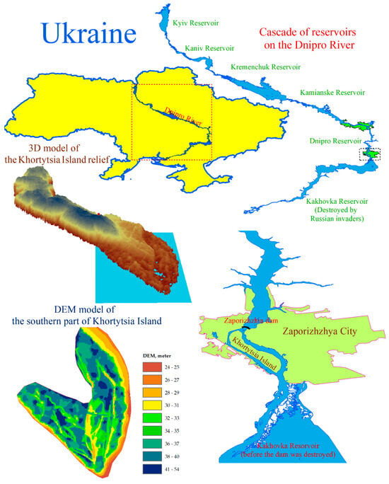
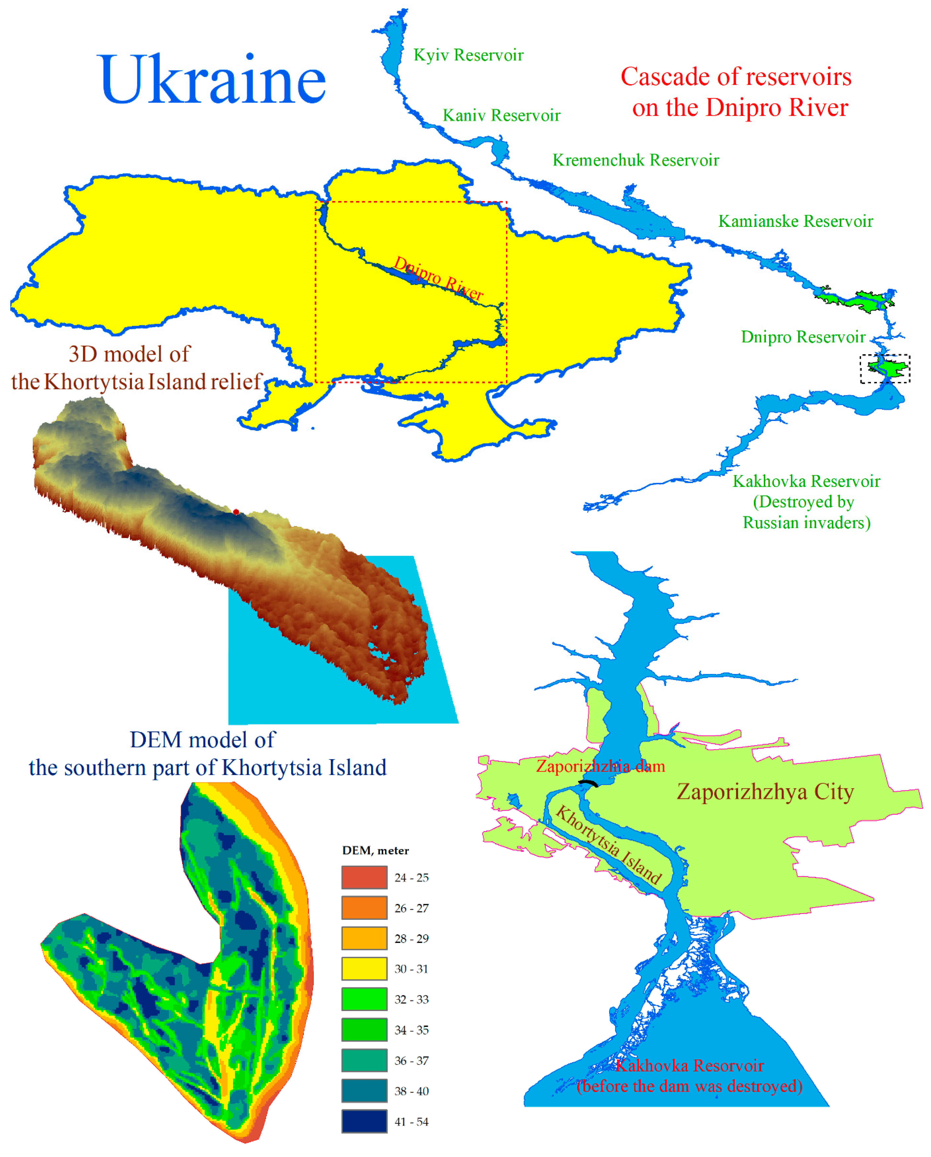
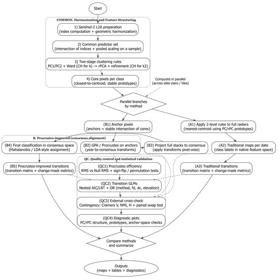
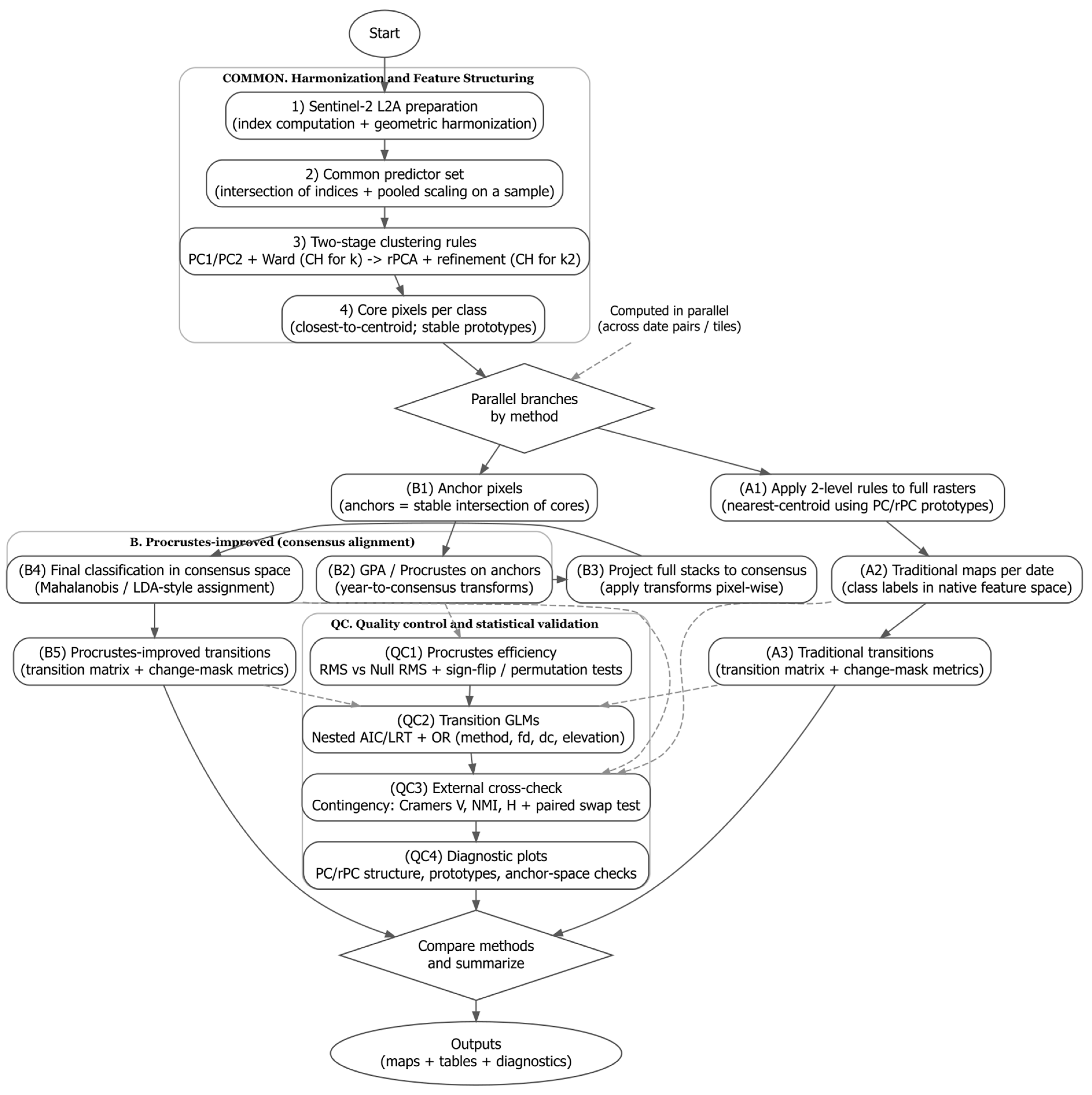
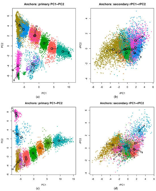
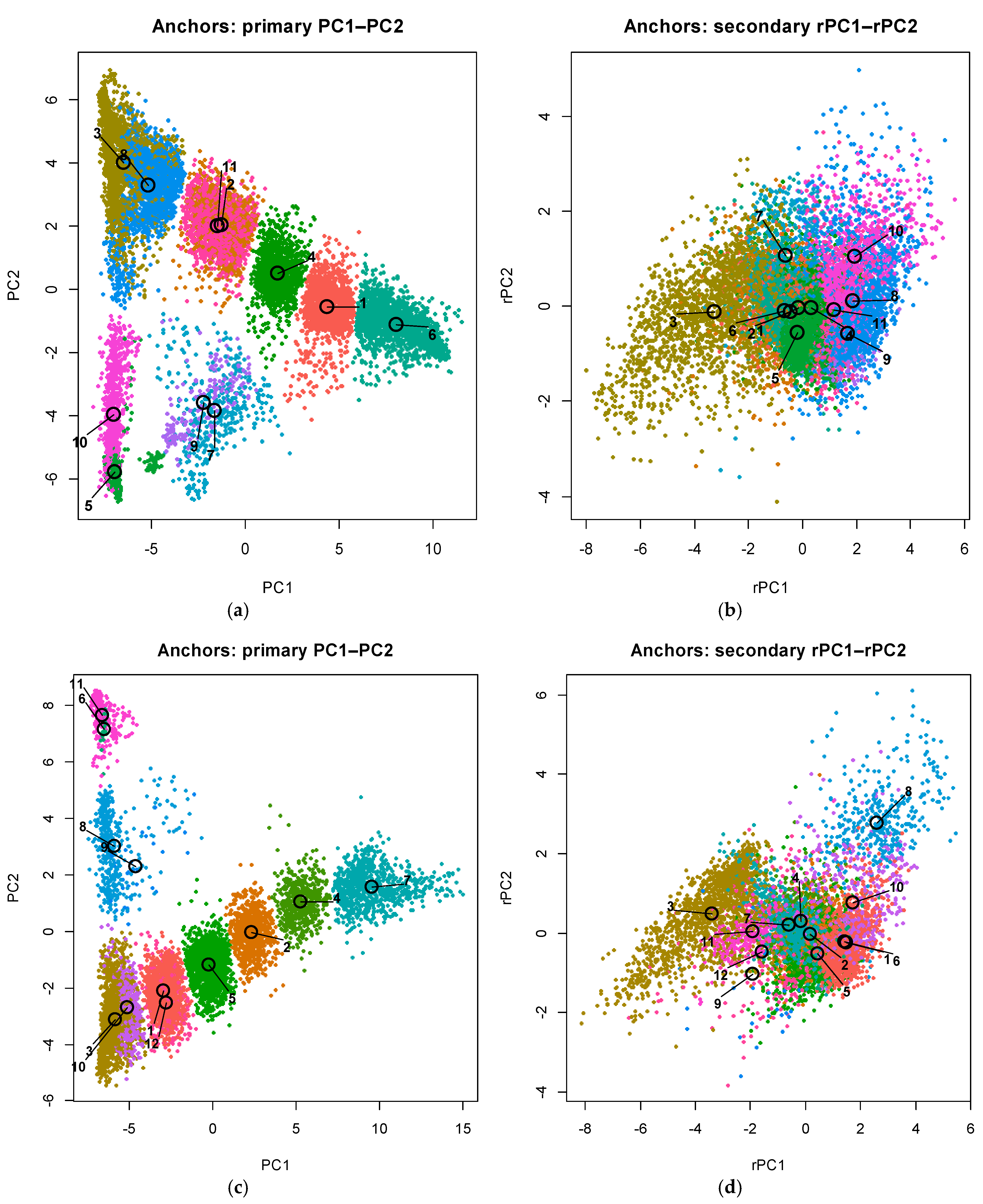
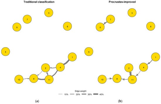
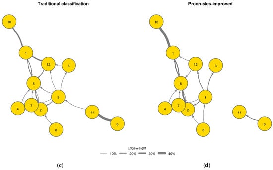
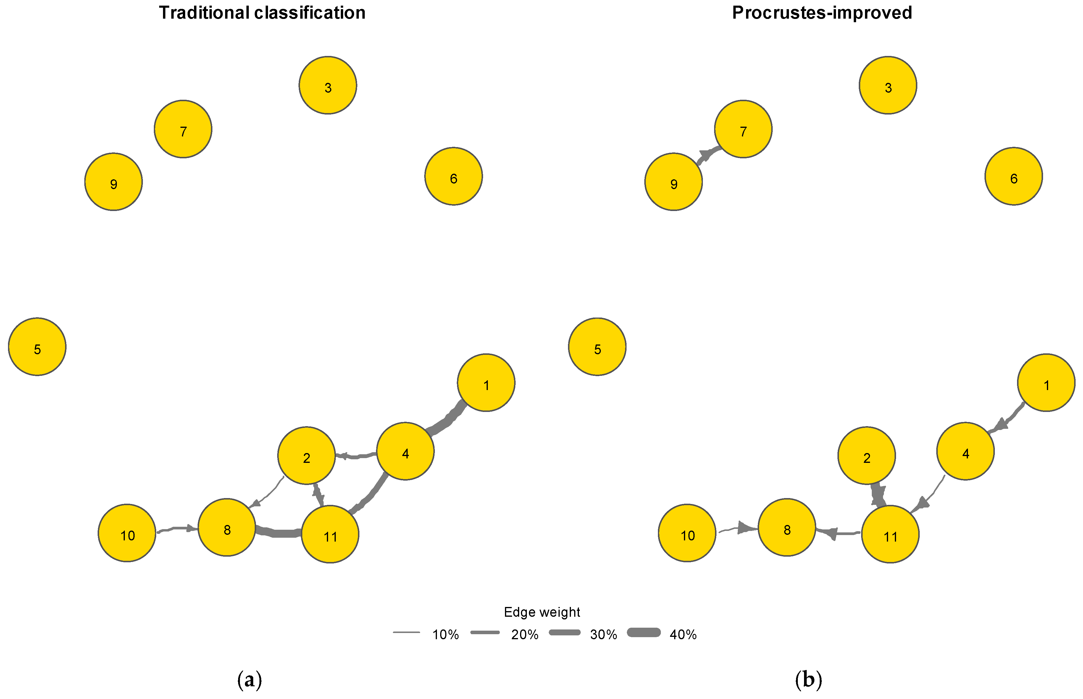
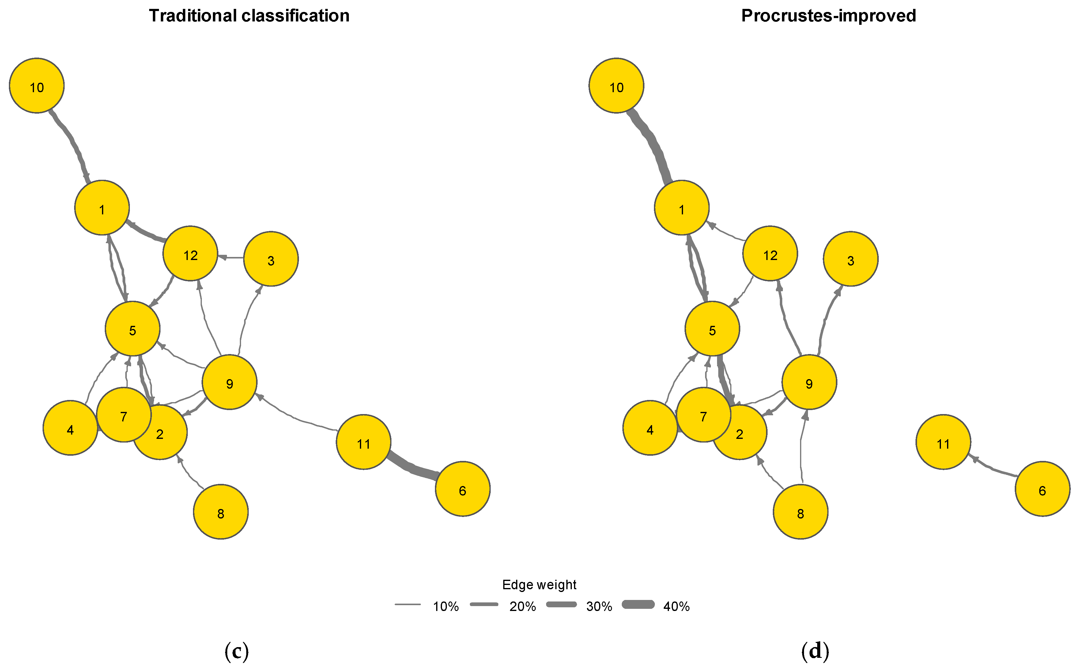
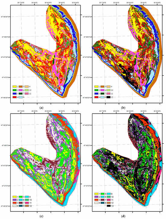
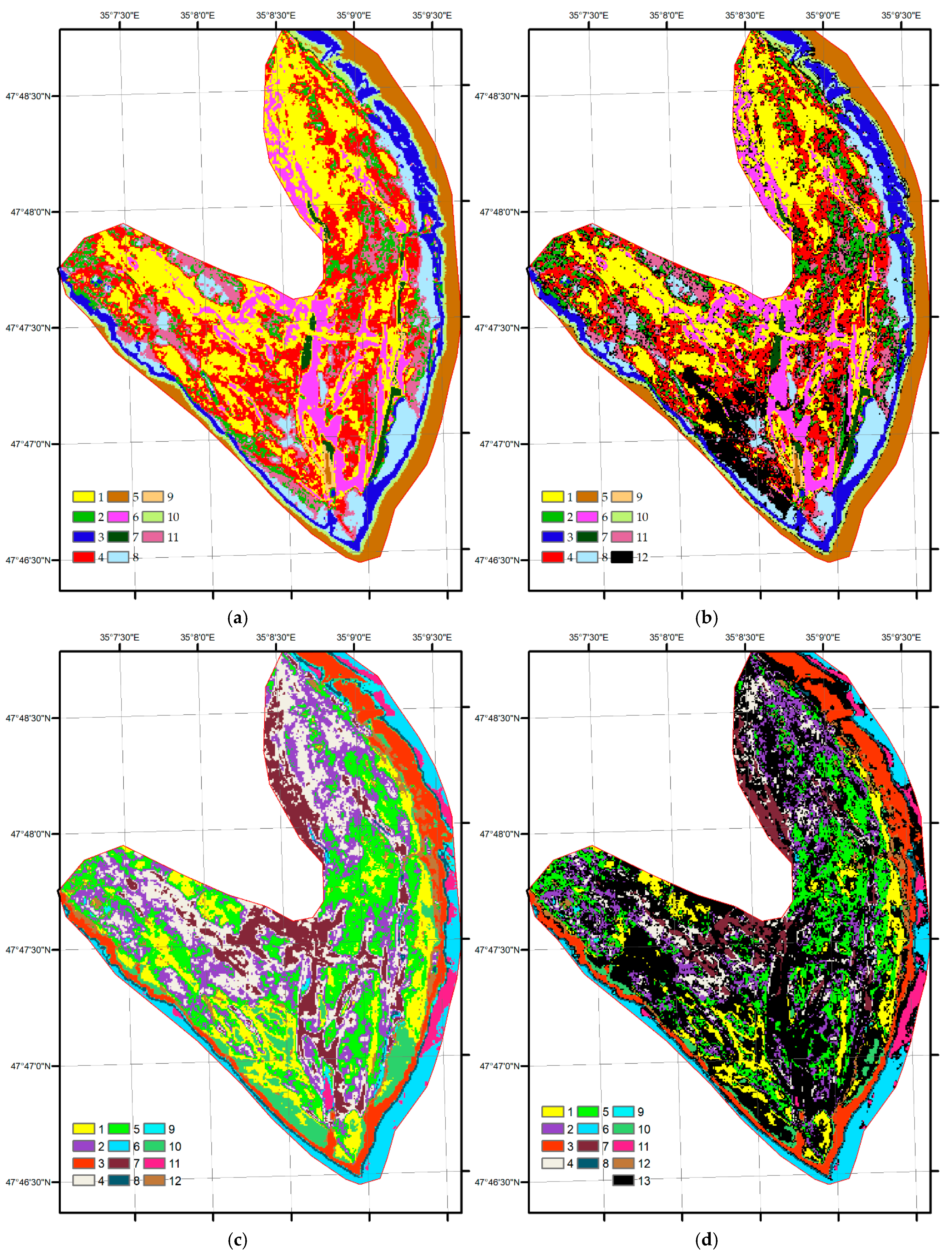
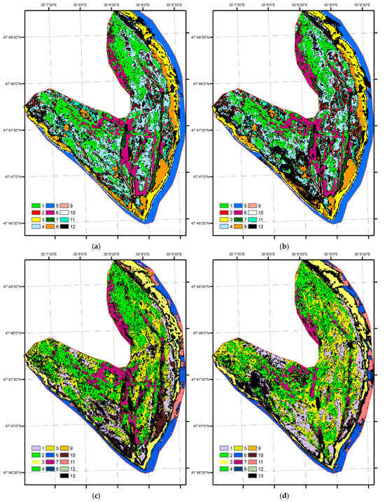
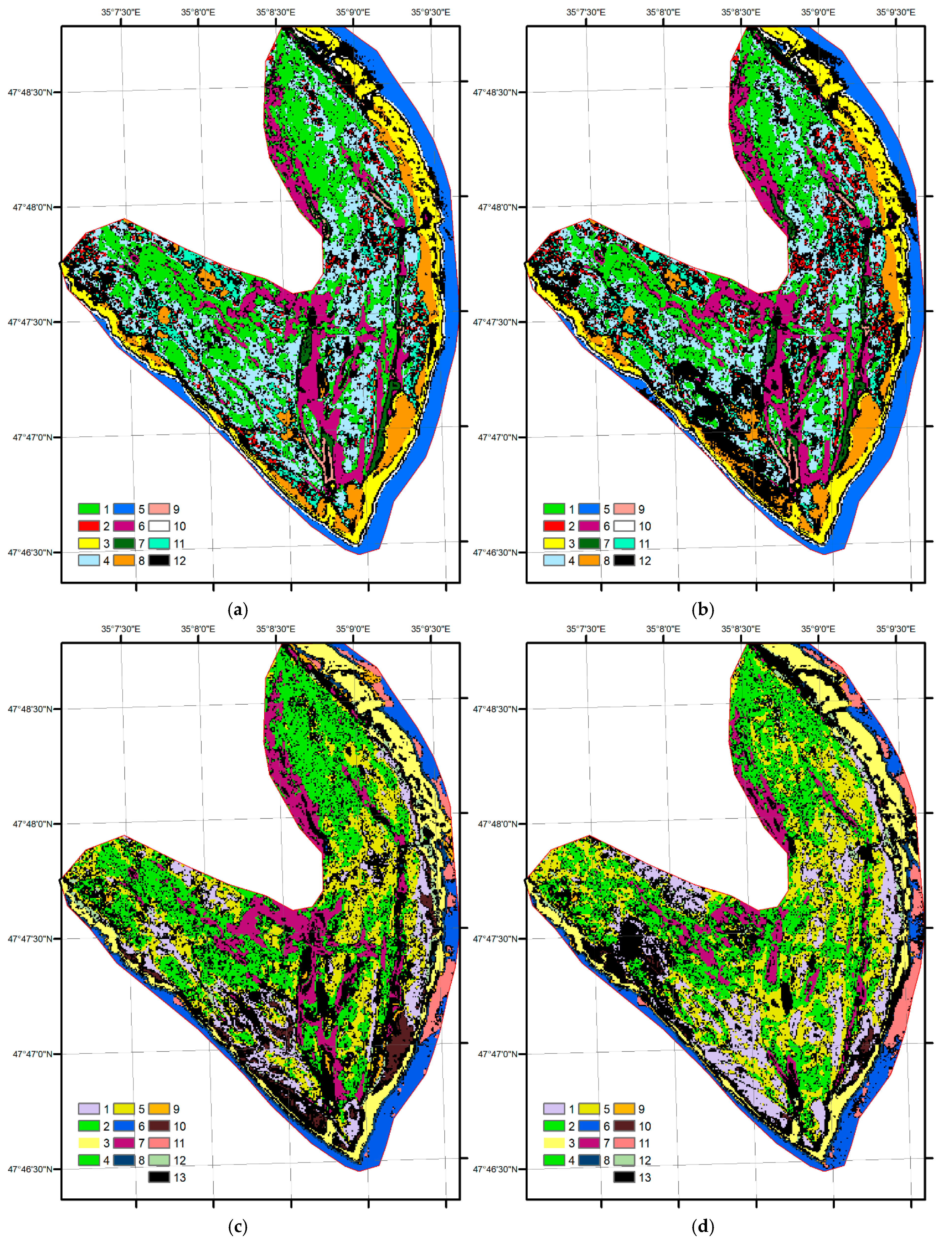

Disclaimer/Publisher’s Note: The statements, opinions and data contained in all publications are solely those of the individual author(s) and contributor(s) and not of MDPI and/or the editor(s). MDPI and/or the editor(s) disclaim responsibility for any injury to people or property resulting from any ideas, methods, instructions or products referred to in the content. |
© 2026 by the authors. Licensee MDPI, Basel, Switzerland. This article is an open access article distributed under the terms and conditions of the Creative Commons Attribution (CC BY) license.