State Evolution and Anomaly Prediction for Selective Laser Melting Multi-Systems Based on Decoupled Spatiotemporal Graph Autoregressive Networks

Abstract

The long-term reliability of selective laser melting (SLM) equipment is constrained by the latent degradation and coupled faults of multiple underlying hardware systems under continuous high-load operations. Transitioning from passive defect detection to proactive prognostics and health management (PHM) is crucial to overcome bottlenecks in industrial applications. Accurately inferring future multi-system hardware states faces three major challenges: feature alignment difficulties under variable-length printing cycles, graph topology collapse under strong industrial noise, and dimensional conflicts along with error cascading divergence during the joint optimization of microscopic physical trajectories (continuous regression) and macroscopic system anomalies (discrete classification) in end-to-end prediction. To address these issues, this paper proposes a decoupled spatiotemporal graph autoregressive network (DS-GAN). First, a multi-scale feature pooling and degradation gating injection mechanism is constructed to align highly variable-length high-frequency sequences and adaptively integrate macroscopic health priors. This approach achieves feature decoupling under physical boundary constraints. Second, a restricted residual graph evolution mechanism is introduced to regulate dynamic coupling drift based on static physical topologies, effectively suppressing feature divergence in the spatial dimension. Finally, a heterogeneous multi-task autoregressive decoder based on homoscedastic uncertainty is designed; this decoder helps reduce the impact of accumulated errors along the time axis during multi-step forecasting. Long-sequence forward inference on a real SLM continuous printing dataset demonstrates that DS-GAN achieves an overall accuracy of 97.48% for multi-system anomalies while strictly limiting the global false alarm rate to 1.85%. Furthermore, quantitative results reveal the physical inertia mechanism within the prediction horizon, demonstrating that the model maintains high fidelity for physical trajectories with a Macro-RMSE of 0.062, even under a maximum predictive horizon of 20 s. This study provides a reliable theoretical and engineering framework for dynamic coupling correlation analysis and proactive fault warning of multi-systems in complex industrial equipment.

1. Introduction

Selective laser melting (SLM) technology has become a core process in high-end manufacturing fields, such as aerospace, due to the ability to directly form complex components [1]. However, SLM equipment experiences extreme thermodynamic and kinetic complexity during continuous manufacturing. Existing condition monitoring studies primarily focus on the post-inspection of forming results or single-dimensional anomaly recognition, failing to deeply analyze the evolution of underlying hardware states during equipment operation [2]. In reality, the physical root causes of processing interruptions and performance degradation usually lie in the latent degradation and multi-physics coupled faults of core hardware subsystems under long-term high-load operations [3]. Physically, these hardware systems do not degrade in isolation but interact through complex thermo-fluidic and opto-thermal mechanisms. For instance, prolonged high-energy laser emission induces thermal lensing effects in the galvanometer optical system, leading to focal shift and energy density attenuation [4]. Simultaneously, the gradual accumulation of spatter and soot in the atmosphere filtration system alters internal aerodynamic pressure dynamics, which directly perturbs the convective heat dissipation efficiency of the cooling circulation [5]. These cascaded physical degradation mechanisms ultimately manifest as dynamic, nonlinear coupling fluctuations in multi-channel sensor time-series. Therefore, constructing a dynamic coupling correlation analysis and health quantification inference model tailored to the multi-system hardware features of SLM equipment is necessary. Such a model facilitates the transition from passive detection to proactive prognostics and health management (PHM), which is a prerequisite for advancing the large-scale engineering applications of SLM.

Accurately inferring future states of multi-system hardware requires analyzing the associated spatial topological coupling mechanisms. The hardware sensing data of SLM equipment manifest as high-frequency and high-dimensional multivariate time series [6]. Traditional time series prediction methods typically flatten multi-source sensor features before inputting them into deep networks. This approach ignores structural isolation boundaries among physical subsystems and easily triggers collinearity traps and mapping distortions among variables in the latent space. Recently, graph neural networks (GNNs) have made significant progress in multivariate time series forecasting by capturing spatial topological dependencies among variables [7]. However, dynamic graph learning methods that rely entirely on data exhibit inherent vulnerabilities. Because these methods assume a completely unknown graph topology, they are prone to node feature over-smoothing and topology collapse under strong industrial high-frequency noise and temporal perturbations. This phenomenon leads to a decline in generalization ability under long-term conditions [8]. Consequently, adaptively quantifying and capturing topological coupling evolution during the multi-field degradation of equipment, while simultaneously introducing physical prior constraints, constitutes a primary challenge in current research.

Long-sequence continuous inference must simultaneously overcome time-axis divergence and multi-objective optimization conflicts. In the temporal dimension, autoregressive inference inherently possesses cumulative effects, where extending the prediction step leads to nonlinear error cascading divergence [9,10]. Traditional two-stage diagnostic methods, which first regressively predict continuous sensor values and then input them into an offline classifier for anomaly diagnosis, sever the backpropagation chain and exacerbate the boundless amplification of front-end errors at the classification stage. In the optimization dimension, utilizing an end-to-end architecture to jointly output microscopic continuous physical trajectories and macroscopic discrete anomaly states represents a typical heterogeneous multi-task learning (MTL) problem. Because mean squared error (MSE) and cross-entropy (CE) losses exhibit absolute differences across magnitudes, applying static weights for linear superposition easily induces gradient conflicts between tasks or backpropagation distortions dominated by a single task. Addressing this structural bottleneck by introducing homoscedastic uncertainty to dynamically balance multi-task losses is an effective mathematical approach to achieve the joint convergence of heterogeneous features [11,12].

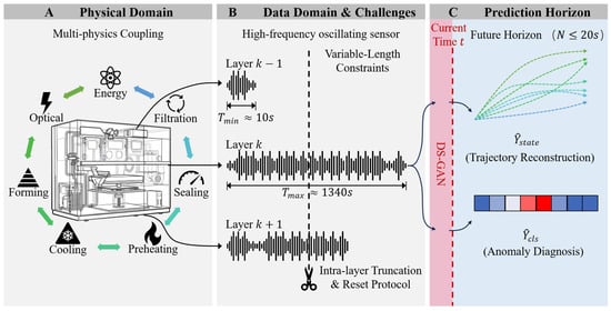
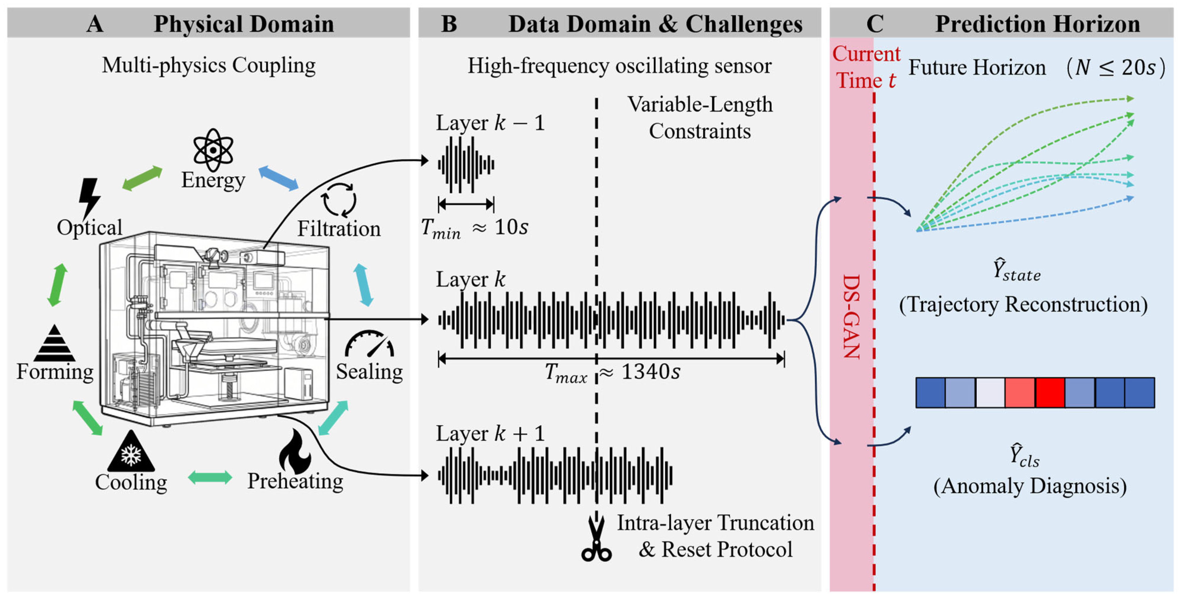
Based on the aforementioned prerequisite constraints and mechanism vulnerabilities, this paper proposes a decoupled spatiotemporal graph autoregressive network (DS-GAN) to solve the dynamic coupling quantification and anomaly traceability prediction problem for multi-system hardware in SLM equipment under variable-length continuous printing cycles, the concept and architecture of which are shown in Figure 1. The main contributions are summarized as follows. First, a physical boundary constraint and macroscopic–microscopic degradation gating injection mechanism is constructed. By safely aligning highly variable-length temporal data within a single layer through multi-scale feature pooling and adaptively allocating the macroscopic health factor representing historical system degradation to microscopic nodes, the proposed approach achieves a deep fusion of cross-scale features while maintaining the physical independence of subsystems. Second, a restricted residual graph evolution mechanism is proposed to suppress topology collapse. By establishing a static physical topology as a defensive baseline, this mechanism regulates the drift of the dynamic coupling graph via learnable inertia weights. It effectively overcomes the robustness defects of pure data-driven graph models under high-frequency industrial noise and suppresses disordered feature divergence in the spatial dimension. Third, a heterogeneous multi-task autoregressive decoder based on homoscedastic uncertainty is designed. By introducing adaptive penalty terms at the mathematical foundation, the decoder endows the network with curriculum learning capabilities to dynamically adjust dimensional gradients, thereby helping reduce the impact of accumulated errors during autoregressive inference. Validation demonstrates that this architecture maintains an overall diagnostic accuracy of 97.48% while keeping the false alarm rate within 1.85%, satisfying industrial deployment standards.

Figure 1. Conceptual framework of multi-system dynamic coupling and health inference for SLM equipment.

2. Related Work and Problem Definition

2.1. State Monitoring and Physical Degradation Inference of SLM Equipment

In the field of selective laser melting (SLM) continuous manufacturing, machine learning-based condition monitoring is a core pathway to enhance equipment reliability. Early studies utilized traditional algorithms for process parameter optimization and threshold alarming [13]. Recently, the introduction of deep learning has expanded monitoring dimensions, but mainstream research remains highly focused on microscopic process feature extraction, such as forming quality analysis and post-inspection based on vision or thermal imaging [14,15]. Such studies mostly remain at the end-to-end mapping level of process parameters to forming quality, lacking a deep analysis of the latent hardware-level degradation of SLM equipment under long-term high-load operations. Although physics-informed hybrid modeling for manufacturing has gradually gained attention [16], proactive joint inference research focusing on dynamic coupling correlations and hardware health quantification of multi-systems in SLM equipment remains in its infancy. There is a lack of theoretical frameworks that effectively integrate microscopic high-frequency fluctuations with macroscopic system degradation.

2.2. Multivariate Time Series Forecasting and Topology Collapse Risks

Multi-system condition monitoring of SLM equipment essentially belongs to high-dimensional and high-frequency multivariate time series (MTS) prediction. Traditional time series models typically assume mutual independence among channels, making the capture of complex spatial thermodynamic and kinetic coupling effects between subsystems difficult. Graph neural networks (GNNs) achieve significant progress in MTS prediction by adaptively capturing implicit spatial dependencies among variables through graph learning modules [17,18]. With further research, dynamic graph neural networks update node topologies in real-time to adapt to time-varying industrial systems [19]. However, dynamic graph architectures relying entirely on data have structural limitations when dealing with strong industrial high-frequency noise. During deep propagation or when facing heterophilic graphs, networks lacking physical prior constraints easily suffer from node feature over-smoothing and topology collapse [20,21], posing severe challenges to robustness under sudden perturbations [22]. Therefore, adaptively capturing topology evolution during multi-field equipment degradation, while simultaneously introducing physical boundary defenses, remains an urgent theoretical difficulty.

2.3. Error Cascading Challenges in Long-Sequence Inference

Future-oriented equipment health assessment relies heavily on long sequence time-series forecasting (LSTF). Currently, attention models represented by Transformers enhance the reconstruction upper bound of LSTF through sparse mechanisms or sequence decomposition [23,24]. Although such architectures perform excellently in time series fitting, the associated autoregressive or direct multi-step inference paradigms easily trigger cumulative effects along the time axis. Research indicates that in the dynamic inference of complex physical fields, extending the prediction step causes prediction deviations to diverge in a nonlinear error cascading manner [25]. Traditional two-stage diagnostic strategies separate the backpropagation chain, causing tiny reconstruction errors at the front end to be boundlessly amplified at the classification end. This limitation fails to meet the engineering requirements for the high-fidelity traceability of future hardware states in SLM continuous printing.

2.4. Heterogeneous Multi-Task Joint Optimization and Dimensional Conflicts

To suppress error cascades, utilizing an end-to-end architecture to jointly output microscopic continuous sensor trajectory reconstructions and macroscopic system anomaly classifications is a feasible approach. However, this architecture inevitably introduces optimization bottlenecks associated with heterogeneous multi-task learning (MTL). Studies indicate that gradients driven by heterogeneous loss functions easily fall into local optima or cancel each other out [26]. Especially in scenarios involving absolute dimensional differences, applying static hyperparameter weights for linear superposition easily triggers gradient domination, where a single task completely dictates network updates. Consequently, employing homoscedastic uncertainty to dynamically weight multi-task losses has been proven to be an effective mathematical strategy for the joint optimization of heterogeneous targets [27,28]. This mechanism endows the network with the ability to adaptively allocate gradients, achieving dynamic blocking and smooth transitions of gradients without manual intervention.

2.5. Problem Definition and Prior Constraints

Current time series inference methods for complex industrial systems, such as SLM, exhibit methodological limitations in addressing topology divergence, error cascading, and multi-task dimensional conflicts. To fill this theoretical gap, this paper constructed an end-to-end inference framework that deeply integrates physical constraints with data-driven approaches. This paper rigorously models hardware state prediction in SLM continuous printing as a variable-length spatiotemporal sequence heterogeneous prediction problem based on physical constraints, establishing the following core priors and variable boundaries. First, regarding the alignment of multi-scale variable-length time windows, assuming the original high-frequency sensor data are ${\mathbf{X}}_{\mathit{raw}}\in {\mathbb{R}}^{B\times L\times T_{\mathit{max}}\times 41}$, the model must adaptively accommodate the maximum single-layer time step T_max to maintain the continuity of the physical degradation envelope, given the physical constraint of unfixed single-layer processing time. Second, for physical grouped dimensionality reduction mapping, to avoid spatial collinearity distortions of the 41-dimensional high-frequency sensing data, the network must strictly decouple and project the input features into 7 microscopic subsystem dimension sets C = {4, 4, 8, 12, 3, 8, 2} according to the true physical configuration of the equipment. Third, concerning macroscopic priors and topological anchoring, before spatiotemporal inference, it is mandatory to introduce a low-frequency macroscopic health factor $\mathbf{HI}\in {\mathbb{R}}^{B\times L\times T_{\mathit{max}}\times 1}$ representing the system-level historical degradation of the equipment and a validated static physical adjacency matrix A_base ∈ ℝ^7×7 to serve as the physical foundation and defensive boundary for dynamic graph evolution. Under this constraint framework, the core inference objective of this paper is to jointly solve the 41-dimensional continuous physical state evolution trajectory and the 8-class macroscopic anomaly state at the future N-th layer, thereby achieving cross-scale equipment hardware health inference and etiology traceability.

3. Decoupled Spatiotemporal Graph Autoregressive Network Architecture

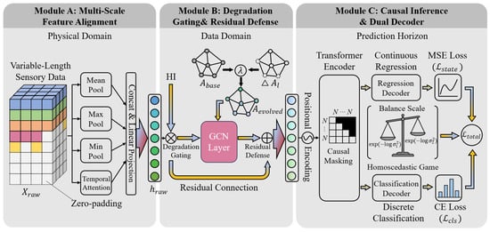
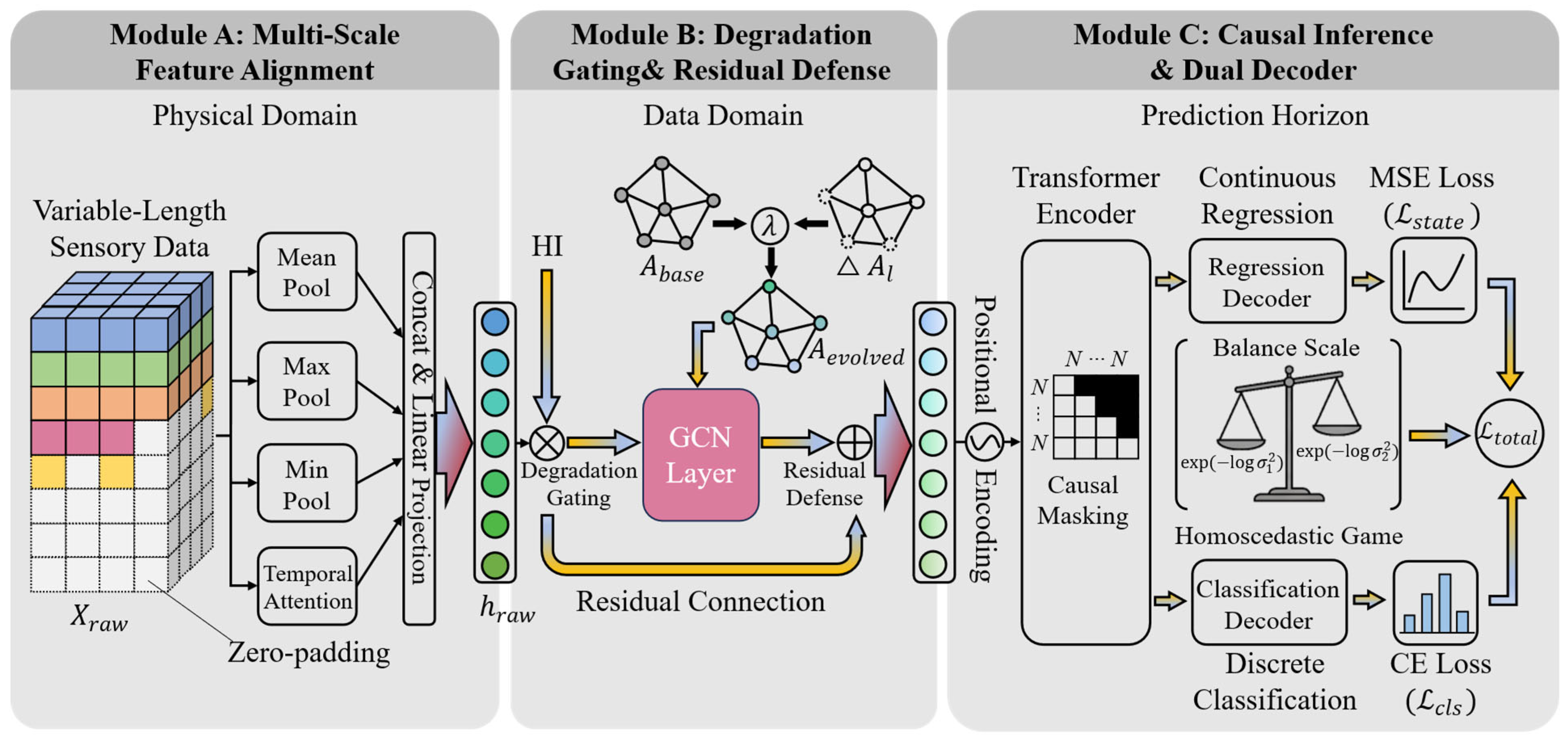
To resolve the problems of strong hardware multi-field coupling, difficulties in extracting long-range evolution features, and multi-task dimensional conflicts in SLM equipment during variable-length continuous printing cycles, this section proposes a decoupled spatiotemporal graph autoregressive network (DS-GAN). This architecture consists of a physical constraint frontend, a degradation gating and graph evolution mid-end, and a heterogeneous multi-task autoregressive decoding backend. The overall architecture is shown in Figure 2.

Figure 2. Overall architecture of the decoupled spatiotemporal graph autoregressive network (DS-GAN).

3.1. Multi-Scale Feature Alignment Under Physical Boundary Constraints

The original condition monitoring data of SLM equipment are high-frequency multivariate time series. Due to the different geometric cross-sectional areas of single-layer printing, the monitoring sequences exhibit significant variable-length characteristics within a single layer. Furthermore, directly flattening and inputting 41-dimensional sensor data into the network easily triggers collinearity traps and mapping distortions lacking physical constraints in the latent space. Therefore, this section first imposes rigid physical boundary constraints and utilizes multi-scale feature pooling to achieve dynamic alignment of the time axis.

Let the raw input tensor first undergo leak-proof normalization. It is crucial to emphasize that zero-padding is applied strictly after normalization to ensure that the padded zeros do not artificially skew the mean and variance of the true physical signals. The normalized sequences are then zero-padded to the adaptive maximum time step T_max, forming ${\mathbf{X}}_{\mathit{raw}}\in {\mathbb{R}}^{B\times L\times T_{\mathit{max}}\times d_{\mathit{raw}}}$, alongside a dynamically generated binary mask ${\mathbf{M}}_{\mathit{mask}}\in {\left\{0, 1\right\}}^{B\times L\times T_{\mathit{max}}\times 1}$ (where 1 indicates valid time steps and 0 indicates padded regions). According to physical priors of the equipment hardware topology, the 41-dimensional features are strictly divided into 7 subsystems, corresponding to the feature channel dimension set C = {4, 4, 8, 12, 3, 8, 2}.

For the microscopic high-frequency sequence ${\mathbf{X}}^i\in {\mathbb{R}}^{B\times L\times T_{\mathit{max}}\times c_i}$ of the i-th subsystem, an independent fully connected layer is first used to project it into a unified latent dimension d_s:

$${\mathbf{X}}^i={\mathbf{X}}^i{\mathbf{W}}_s^i+{\mathbf{b}}_s^i$$

(1)

To eliminate the interference of invalid zero-padding regions and extract the microscopic physical envelope within a single layer, multi-scale statistical pooling and temporal attention pooling are executed in parallel. A local binary mask ${\mathbf{M}}^i\in {\left\{0, 1\right\}}^{T_{\mathit{max}}}$ is explicitly defined for this subsystem:

$${\mathbf{M}}_t^i=\left\{\begin{array}{cc}1,& \mathrm{if} \mathit{t} \mathrm{is\; a\; valid\; step}\\ 0,& \mathrm{if} \mathit{t} \mathrm{is\; a\; padded\; step}\end{array}\right.$$

(2)

To prevent padded zeros from incorrectly pulling down the mean or being identified as the physical extremum, the mask is mathematically applied to the pooling operations. For mean pooling, the sum is divided only by the count of valid steps. For max and min pooling, masked values are replaced by −∞ and +∞, respectively, before the operation:

$${\mathbf{h}}_{\mathit{mean}}^i={\displaystyle \frac{{\displaystyle {\sum }_{t=1}^{T_{\mathit{max}}}}{\mathbf{X}}_t^i\odot {\mathbf{M}}_t^i}{{\displaystyle {\sum }_{t=1}^{T_{\mathit{max}}}}{\mathbf{M}}_t^i}}$$

(3)

$${\mathbf{h}}_{\mathit{max}}^i={\mathit{max}}_t\left({\mathbf{X}}_t^i\odot {\mathbf{M}}_t^i-\infty \cdot (1-{\mathbf{M}}_t^i)\right)$$

(4)

$${\mathbf{h}}_{\mathit{min}}^i={\mathit{min}}_t\left({\mathbf{X}}_t^i\odot {\mathbf{M}}_t^i+\infty \cdot (1-{\mathbf{M}}_t^i)\right)$$

(5)

For temporal attention, a large negative penalty (−∞) is added to the pre-softmax scores of padded steps, ensuring that their attention weights α_t strictly evaluate to zero:

$${\alpha }_t=\mathrm{Softmax}\left({\mathbf{W}}_2\tanh \left({\mathbf{W}}_1{\mathbf{X}}_t^i\right)-\infty \cdot \left(1-{\mathbf{M}}_t^i\right)\right)$$

(6)

$${\mathbf{h}}_{\mathit{att}}^i={\sum }_{t=1}^{T_{\mathit{max}}}{\alpha }_t\odot {\mathbf{X}}_t^i$$

(7)

Finally, a feature fusion layer concatenates the aforementioned multi-scale features along the feature dimension, reducing the dimensionality to output the time-aligned representation of this subsystem:

$${\mathbf{h}}_{\mathit{pool}}^i=\mathrm{Linear}\left({\mathbf{h}}_{\mathit{mean}}^i\left|\right|{\mathbf{h}}_{\mathit{max}}^i\left|\right|{\mathbf{h}}_{\mathit{min}}^i\left|\right|{\mathbf{h}}_{\mathit{att}}^i\right)$$

(8)

Through this module, original variable-length high-frequency sequences are safely compressed and aligned into equal-length and physically mutually independent node feature tensors ${\mathbf{H}}_{\mathit{pool}}\in {\mathbb{R}}^{B\times L\times 7\times d_h}$.

3.2. Degradation Gating Injection Driven by Macroscopic and Microscopic States

After obtaining the microscopic features of each subsystem, they must be physically aligned with the global macroscopic health factor HI. As a low-frequency scalar reflecting the overall degradation degree of the equipment, HI quantifies the accumulated hardware damage under multi-system coupling. To clarify its practical construction, HI is derived exclusively from the real-time multivariate sensing signals acquired up to the current prediction time t. It is strictly an unsupervised metric, ensuring that no future temporal data or discrete anomaly labels are involved in its construction. Specifically, HI is calculated based on the statistical Mahalanobis distance between the current multi-dimensional sensor data and a pre-calibrated healthy baseline established during the initial normal printing stage. To prevent high-frequency transient noise from distorting the degradation baseline, this distance is rigorously smoothed through a low-pass moving average filter. In an actual online monitoring deployment, this indicator is computed sequentially at the raw sampling frequency and aggregated to 1 Hz, providing a continuously updated, real-time macroscopic context for the network. To prevent high-dimensional microscopic features from obscuring these robust low-dimensional macroscopic priors, this paper constructs a degradation gating injection mechanism.

Let the global macroscopic features after mean pooling along the time axis be h_macro ∈ ℝ^B×L×1. For the i-th microscopic physical node, a gating activation vector Gⁱ based on Query-Key similarity is constructed:

$${\mathbf{G}}^i=\sigma \left({\mathbf{W}}_q{\mathbf{h}}_{\mathit{pool}}^i+{\mathbf{W}}_k{\mathbf{h}}_{\mathit{macro}}\right)$$

(9)

where σ(⋅) is the Sigmoid activation function. This gating vector performs adaptive weight truncation on the Value mapping of the macroscopic state, and it is deeply concatenated with microscopic features to form the initial spatial graph node feature ${\mathbf{H}}_0^i$:

$${\mathbf{h}}_{\mathit{inject}}^i={\mathbf{G}}^i\odot \left({\mathbf{W}}_v{\mathbf{h}}_{\mathit{macro}}\right)$$

(10)

$${\mathbf{H}}_0^i={\mathbf{W}}_{\mathit{fuse}}({\mathbf{h}}_{\mathit{pool}}^i\left|\right|{\mathbf{h}}_{\mathit{inject}}^i)$$

(11)

The physical mapping relationship of this mechanism uses the microscopic physical state as a Query to adaptively regulate the degradation feature weights integrated from the global decay HI for local nodes. Under the premise of maintaining subsystem independence, it achieves adaptive allocation of system-level decay to local hardware.

3.3. Restricted Residual Graph Evolution Mechanism

Although the static reference graph A_base ∈ ℝ^7×7 established based on physical configuration priors (constructed via a deterministic binary mapping of the hardware PLC control logic and thermodynamic layout interconnectivity) defines the standard coupling structure among subsystems, the coupling weights between systems dynamically drift during the continuous printing degradation process. Physically, this topological drift originates from the cross-domain propagation of degradation. For example, as filter clogging increases aerodynamic resistance, the dominant heat dissipation bottleneck shifts from normal cooling logic to pressure-induced thermo-fluidic constraints, causing the sensor correlation (i.e., graph edges) between the filtration and cooling nodes to strengthen nonlinearly. To capture this physical evolution characteristic while preventing the topology structure collapse of pure data-driven graph models under strong industrial noise, a restricted residual graph evolution mechanism is introduced.

Using the node feature tensor ${\mathbf{H}}_0\in {\mathbb{R}}^{B\times L\times 7\times d_{\mathit{model}}}$ output from the previous stage, a real-time dynamic topology perturbation matrix ΔA_l for the current layer is generated through scaled dot-product attention:

Q = H₀W_Q,  K = H₀W_K

(12)

$$\Delta {\mathbf{A}}_l=\mathrm{Softmax}\left({\displaystyle \frac{\mathbf{Q}{\mathbf{K}}^T}{\sqrt{d_{\mathit{model}}}}}\right)$$

(13)

Subsequently, a learnable inertia constraint coefficient λ = σ(λ_logit) is introduced to construct the restricted residual topology equation:

A_evolved = λA_base + (1 − λ)ΔA_l

(14)

Equation (14) mathematically establishes a rigorous tolerance mechanism against physical prior sensitivity. If the pre-determined A_base contains inappropriate physical definitions or inherent structural flaws, the network autonomously penalizes the gradient of the inertia coefficient λ during backpropagation. This shifts the topological dominance toward the data-driven perturbation ΔA_l, thereby preventing rigid or erroneous prior constraints from distorting downstream autoregressive state trajectories. After computing the evolved graph structure, spatial graph convolutions are executed to complete information interactions among the 7 subsystem nodes. Feature residual connections are added to suppress the over-smoothing phenomenon during deep network propagation:

H_graph = ReLU(A_evolved(H₀W_V)) + H₀

(15)

3.4. Causal Inference with Heterogeneous Multi-Task Joint Optimization

Node features that have undergone spatial topological interactions are flattened, and temporal information is injected through positional encoding: H_seq = PE(Flatten(H_graph)). By deploying an autoregressive Transformer encoder employing causal masking, the evolution feature representation ${\mathbf{H}}_{\mathit{future}}\in {\mathbb{R}}^{B\times N\times 7\times d_{\mathit{model}}}$ for the future N steps is inferred. Specifically, the forecasting workflow adopts a recursive (step-by-step) autoregressive strategy. During the training phase, standard teacher forcing is utilized, where the ground-truth physical values of previous steps are fed into the causal mask to predict the next step, thereby ensuring stable gradient descent. During the inference phase, the model operates purely recursively, feeding its own predicted trajectory output at step t back into the network as the input for step t + 1. To explicitly illustrate the integration of this recursive mechanism with the dual-decoder architecture, the exact training and inference workflows are summarized in Algorithm 1.

Algorithm 1: Training and Inference Workflow of DS-GAN

Input: Historical observation graph nodes Hgraph, Ground truth future trajectory Ystate, Prediction horizon N;

Output: Predicted continuous trajectory ${\hat{\mathbf{Y}}}_{\mathit{state}}$, Discrete classification distribution ${\hat{\mathbf{Y}}}_{\mathit{cls}};$

Phase 1: Training Stage (Teacher Forcing)

1: Initialize causal mask to prevent forward temporal information leakage

2: for step i = 1 to N do

3:  Extract sequence representation ${\mathbf{H}}_{\mathit{seq}}^i$ using historical states and ground truth ${\mathbf{Y}}_{\mathit{state}}^{\left(1:i-1\right)}$

4:  Decode continuous regression state ${\hat{\mathbf{Y}}}_{\mathit{state}}^i$

5: end for

6: Decode classification distribution ${\hat{\mathbf{Y}}}_{\mathit{cls}}$ using the node-fused final state ${\mathbf{H}}_{\mathit{seq}}^N$

7: Calculate dynamic homoscedastic joint loss $ℒ$total using Equation (18)

8: Backpropagate $ℒ$total to update network weights and log-variance parameters

Phase 2: Inference Stage (Recursive Forecasting)

9: Initialize causal mask

10: for step i = 1 to N do

11:  Extract sequence representation ${\mathbf{H}}_{\mathit{seq}}^i$ using historical states and previously predicted ${\hat{\mathbf{Y}}}_{\mathit{state}}^{\left(1:i-1\right)}$

12:  Decode continuous regression state ${\hat{\mathbf{Y}}}_{\mathit{state}}^i$

13: end for

14: Decode classification distribution ${\hat{\mathbf{Y}}}_{\mathit{cls}}$ using the final predicted state ${\mathbf{H}}_{\mathit{seq}}^N$

15: return ${\hat{\mathbf{Y}}}_{\mathit{state}}$ and ${\hat{\mathbf{Y}}}_{\mathit{cls}}$

To address the issue where traditional two-stage predictions easily trigger time-axis error cascading divergence, DS-GAN branches into a heterogeneous multi-task dual decoder at the network backend. The continuous trajectory reconstruction branch for physical states independently maps each node feature to output the 41-dimensional sensor normalized evolution trajectory ${\hat{\mathbf{Y}}}_{\mathit{state}}$ for the future N steps. The corresponding loss function adopts mean squared error (MSE):

$${\mathcal{L}}_{\mathit{state}}={\displaystyle \frac{1}{M}}\sum {\left({\hat{\mathbf{Y}}}_{\mathit{state}}-{\mathbf{Y}}_{\mathit{state}}\right)}^2$$

(16)

The discrete classification branch for future system anomalies extracts node-fused spatial features at the end of the prediction horizon to directly map them into an 8-dimensional classification prediction distribution ${\hat{\mathbf{Y}}}_{\mathit{cls}}$. The corresponding loss function adopts cross-entropy (CE):

$${\mathcal{L}}_{\mathit{cls}}=\mathrm{CrossEntropy}\left({\hat{\mathbf{Y}}}_{\mathit{cls}},{\mathbf{Y}}_{\mathit{cls}}\right)$$

(17)

Considering the significant dimensional differences between continuous regression and discrete classification, applying fixed-weight linear superposition easily leads to gradient update distortion. Therefore, this paper introduces a homoscedastic uncertainty joint optimization objective. Two learnable log-variance parameters $\log \left({\sigma }_1^2\right)$ and $\log \left({\sigma }_2^2\right)$ are defined to construct an adaptive loss function:

$${\mathcal{L}}_{\mathit{total}}={\displaystyle \frac{1}{\exp \left(\log \left({\sigma }_1^2\right)\right)}}{\mathcal{L}}_{\mathit{state}}+\log \left({\sigma }_1^2\right)+{\displaystyle \frac{1}{\exp \left(\log \left({\sigma }_2^2\right)\right)}}{\mathcal{L}}_{\mathit{cls}}+\log \left({\sigma }_2^2\right)$$

(18)

During backpropagation, the network adaptively adjusts log-variance penalty terms based on the current fitting error and gradient state of each task. At the mathematical foundation, this mechanism endows the model with curriculum learning capabilities to dynamically allocate computation weights, effectively mitigating the one-way transmission of front-end reconstruction errors to the backend and ensuring the joint stable convergence of multi-dimensional heterogeneous tasks.

4. Experimental Design and Result Analysis

4.1. Variable-Length Period Dataset Reconstruction and Experimental Settings

To verify the predictive capabilities of the proposed decoupled spatiotemporal graph autoregressive network (DS-GAN) in real industrial scenarios, the data used in this experiment originates from a continuous printing condition monitoring platform of SLM equipment. The dataset contains 390,220 continuously collected second-level multivariate sensing time series data entries, fully covering the working cycles of 8582 forming layers. The feature space encompasses 41-dimensional multi-physics sensor parameters across 7 key hardware subsystems, along with the 1-dimensional macroscopic degradation health factor HI output by the model frontend [3,4]. To clarify the engineering context and specific physical significance of the acquired signals, Table 1 summarizes the physical variables associated with these 41 sensors, along with their corresponding core components and subsystems; all high-frequency raw signals were time-aligned and aggregated to 1 Hz to construct a dataset for second-level assessment.

Table 1. Configuration and physical meaning of the 41-dimensional sensing variables.

Subsystem	Component	Key Parameters (Variables)
Optical	Galvanometer	Voltage, Temperature, Humidity, Head Temperature
Cooling	High-Temperature Water	Temperature, Flow Rate
	Low-Temperature Water	Temperature, Flow Rate
Forming	Build Cylinder	Current Position, Current Velocity, Right-Side Position, Torque
	Recoater Blade	Current Position, Current Velocity
	Powder Delivery	Feed Multiplier, Weight
Sealing	Processing Chamber	Pressure, Oxygen Concentration 1, 2
	Main Circuit	Inlet Air Velocity, Pressure, Temperature
		Return Air Velocity, Pressure, Temperature
	Branch Circuit	Return Air Velocity, Pressure, Temperature
Preheating	Substrate Plate	Temperature (Zones 1, 2, 3)
Filtration	Pressure	Total Inlet Air, Backblow Air, Compressed Air
	Inlet Air Flow	Rear Panel, Main Chamber, Protective Window
	Differential Pressure	Coarse Filter 1, 2
Energy	Lasers	Actual Power (Laser 1, 2)

Regarding the labeling methodology for the 8 condition classes, the ground truth was rigorously established through cross-verification of the equipment’s PLC event logs, threshold-based hardware alarms, and subsequent manual maintenance records. Specifically, Class 0 represents the Normal operating state, while Classes 1 to 7 represent explicit anomaly events or degradation limits triggered within their respective subsystems. To reflect the inherent long-tail anomaly distribution in actual industrial production, the dataset preserves its natural imbalance. Table 2 summarizes the data distribution of Classes 0–7; this authentic imbalanced context further justifies the necessity of the proposed homoscedastic multi-task joint optimization mechanism in preventing the network from collapsing into the majority class.

Table 2. Data distribution in subsystems.

Dataset	Normal (Y = 0)	Optical (Y = 1)	Cooling (Y = 2)	Forming (Y = 3)	Sealing (Y = 4)	Preheating (Y = 5)	Filtration (Y = 6)	Energy (Y = 7)
Quantity	290,220	1960	1960	3900	5840	1460	3900	980

During the continuous additive manufacturing process, influenced by dynamic changes in the cross-sectional areas of 3D models, the actual printing time of a single layer exhibits significant time-varying fluctuation characteristics. Traditional fixed-window truncation methods destroy the integrity of the hardware physical operation envelope. Therefore, this experiment adopts an adaptive time-step padding strategy during the data preprocessing stage. It first extracts the global maximum single-layer processing time T_max. Then, it reconstructs and zero-pads the variable-length time series data into normalized tensors X_norm and M_mask, which are subsequently input into the temporal attention pooling layer at the network frontend for dynamic feature extraction.

To prevent data leakage vulnerabilities inherent in time series prediction tasks, the experiment discards random cross-validation and adopts a strict chronological sliding split. Following the chronological evolution order, the first 70% of the layer sequences are used as the training set, while the remaining 30% serve as an independent test set. The sliding historical observation window length is set to L_h layers. To explicitly clarify the multi-scale temporal relationships, a layer denotes the continuous printing cycle for a single 3D physical cross-section. Within each layer, the raw high-frequency signals are aggregated into second-level data (i.e., a 1 Hz sampling rate). Consequently, the temporal resolution of the model’s sequence is exactly 1 s per step. For the forward prediction phase, a prediction step N corresponds precisely to N seconds into the future. The model is evaluated within an effective predictive horizon (EPH) of up to N = 20 s, aligning with practical PLC emergency intervention lead times.

Crucially, to address the non-continuous phase transition caused by the rigid non-processing time (recoating and platform lowering) between layers, this study implemented an Intra-layer Truncation and Reset Protocol. Forward prediction strictly operates within the continuous laser emission period where physical fields evolve naturally. When the sliding window encounters a layer boundary, the continuous evaluation is truncated, and the model’s microscopic high-frequency latent state is cleared and reset using the new layer’s topological baseline A_base. It is critical to emphasize that this reset protocol does not erase the long-term physical memory of the equipment. While the high-frequency temporal dependencies are severed to mathematically avoid non-differentiable error jumping during non-processing intervals (e.g., recoating), the cross-layer progressive degradations—such as heat accumulation across consecutive layers, gradual lens debris contamination, and continuous mechanical wear—are captured and continuously inherited through the global macroscopic health factor HI. As defined in Section 3.2, HI acts as a slow-varying state variable that traverses multiple layers. At the beginning of each new layer, this accumulated multi-layer degradation prior is adaptively re-injected into the reset microscopic nodes via the degradation gating mechanism, thereby ensuring the unbroken continuity of macro-scale physical degradation. This protocol physically prevents cross-layer topological collapse and mathematically avoids non-differentiable error jumping during non-processing intervals.

Finally, to facilitate model reproducibility, the main training settings and hyperparameter configurations are summarized in Table 3. The network is optimized using the AdamW optimizer coupled with a cosine annealing learning rate schedule to stabilize the heterogeneous multi-task convergence.

Table 3. Summary of Main Training Settings and Hyperparameters.

Parameter/Setting	Description/Value
Historical Observation Window (Lh)	5 layers
Maximum Single-Layer Time Step (Tmax)	1340 s
Sequence Latent Dimension (ds)	64
Model Hidden Dimension (dmodel)	128
Optimizer	AdamW (β1 = 0.9, β2 = 0.999)
Base Learning Rate	1 × 10−4 (Cosine Annealing)
Batch Size (B)	32
Training Epochs	100

4.2. Baseline Models and Evaluation Metric System

To systematically ablate the contributions of various modules in the DS-GAN architecture, this experiment constructs a baseline model matrix. Baseline 1 is the Vanilla Transformer. It removes the spatial graph convolution and HI gating mechanisms, directly performing autoregressive inference after flattening the 41-dimensional features to establish a prediction performance lower bound without physical spatial constraints. Baseline 2 is MTGNN. As a benchmark for pure data-driven graph networks, this model does not introduce the physical prior graph A_base and relies entirely on data to learn node topology, validating the necessity of physical prior defenses in resisting long-term industrial noise and topology collapse. Baseline 3 is the Two-Stage Cascade DS-GAN. It blocks the joint backpropagation of heterogeneous multi-tasks, predicting future sensor trajectories in the first stage and inputting the trajectories into an offline classifier in the second stage to evaluate the advantage of the end-to-end architecture in suppressing error cascades. Baseline 4 is the Fixed-Weight DS-GAN. It retains the overall network topology but removes the homoscedastic uncertainty mechanism, forcibly anchoring the loss weights of continuous regression and discrete classification at a one-to-one ratio to demonstrate the critical role of the adaptive multi-task mechanism in resolving gradient dimensional conflicts.

Regarding evaluation metrics, this study defines two sets of quantitative evaluation systems for heterogeneous multi-task outputs. For the continuous trajectory reconstruction of microscopic physical states, root mean square error (RMSE) and mean absolute error (MAE) are adopted to measure spatiotemporal fidelity:

$$\mathrm{RMSE}=\sqrt{{\displaystyle \frac{1}{\mathrm{M}}}{\displaystyle \sum _{\mathrm{m}=1}^{\mathrm{M}}}{\left({\mathrm{y}}_{\mathrm{m}}-{\hat{\mathrm{y}}}_{\mathrm{m}}\right)}^2}$$

(19)

$$\mathit{MAE}={\displaystyle \frac{1}{M}}{\displaystyle \sum _{m=1}^M}\left|y_m-{\hat{y}}_m\right|$$

(20)

where M is the product of total prediction steps and feature channels, while y_m and ${\hat{y}}_m$ are the true physical value and model predicted value at the future N-th step, respectively. For the discrete classification of macroscopic equipment system anomalies, detection rate (DR), precision, and F1-score are utilized for subsystem traceability evaluation. For the i-th class subsystem:

$$D{R}_i={\displaystyle \frac{T{P}_i}{T{P}_i+F{N}_i}}$$

(21)

$${\mathit{Precision}}_i={\displaystyle \frac{T{P}_i}{T{P}_i+F{P}_i}}$$

(22)

$$F{1}_i=2\times {\displaystyle \frac{{\mathit{Precision}}_i\times D{R}_i}{{\mathit{Precision}}_i+D{R}_i}}$$

(23)

Additionally, the global false alarm rate (FAR) is introduced to assess the reliability of industrial deployment:

$$\mathit{FAR}={\displaystyle \frac{F{P}_{\mathit{total}}}{F{P}_{\mathit{total}}+T{N}_{\mathit{total}}}}$$

(24)

where TP, FP, FN, and TN represent the numbers of true positives, false positives, false negatives, and true negatives, respectively.

4.3. Fidelity Analysis of Physical State Spatiotemporal Evolution Trajectories

In the heterogeneous prediction architecture, the accurate reconstruction of microscopic physical continuous variables is a prerequisite for ensuring the accuracy of long-term discrete anomaly classification. In autoregressive inference tasks, as the prediction step N increases, time series models lacking spatial topological constraints usually experience nonlinear divergence due to error accumulation. To verify the inference fidelity of DS-GAN under different future time windows within the effective predictive horizon, this section extracts the root mean square error (Z-score standardized) at various steps, with results shown in Table 4.

Table 4. RMSE evolution trends of physical state reconstruction under different prediction steps N (seconds).

Category	Subsystem	N = 5	N = 10	N = 15	N = 20
Class 5	Preheat	0.010	0.015	0.021	0.028
Class 0	Normal	0.013	0.019	0.025	0.033
Class 2	Cooling	0.016	0.022	0.029	0.038
Class 6	Filtration	0.020	0.027	0.035	0.045
Class 4	Sealing	0.025	0.034	0.044	0.056
Class 7	Energy	0.032	0.045	0.060	0.078
Class 1	Optical	0.038	0.054	0.073	0.095
Class 3	Forming	0.048	0.070	0.095	0.124
Macro-RMSE		0.025	0.035	0.047	0.062

Regarding the suppression of error cascades in macroscopic spatiotemporal inference, global metrics indicate that when the prediction step extends from N = 5 to N = 20, the global average Macro-RMSE merely increases from 0.025 to 0.062. By constraining the maximum step to N = 20 under the Intra-layer Truncation Protocol, the prediction error of DS-GAN exhibits highly robust sub-exponential growth characteristics, effectively mitigating the uncontrollable divergence typically seen in unbounded autoregression within the evaluated 20-s horizon. This fidelity advantage is primarily attributed to the restricted residual graph evolution mechanism at the model frontend. During inference, prediction features are anchored by the physical reference topology graph A_base, and the learnable inertia weight λ (as defined in Equation (14)) effectively suppresses the amplification of local high-frequency noise in the autoregressive loop, ensuring that the overall physical evolution envelope of the system does not drift.

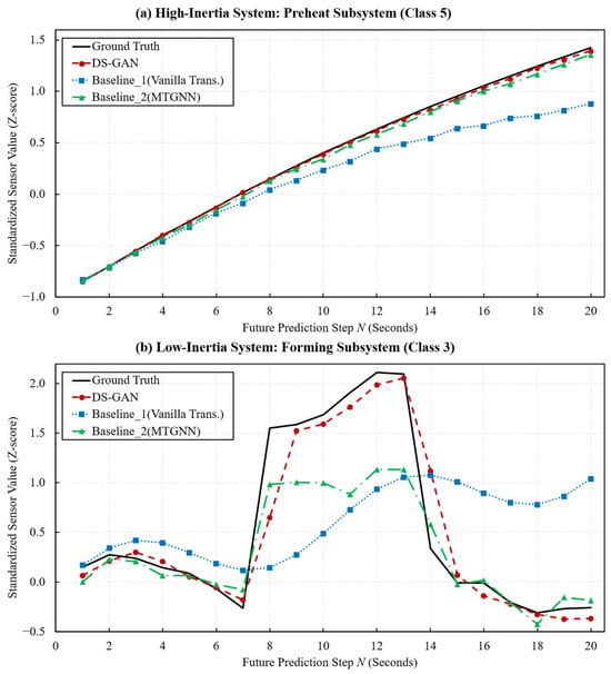
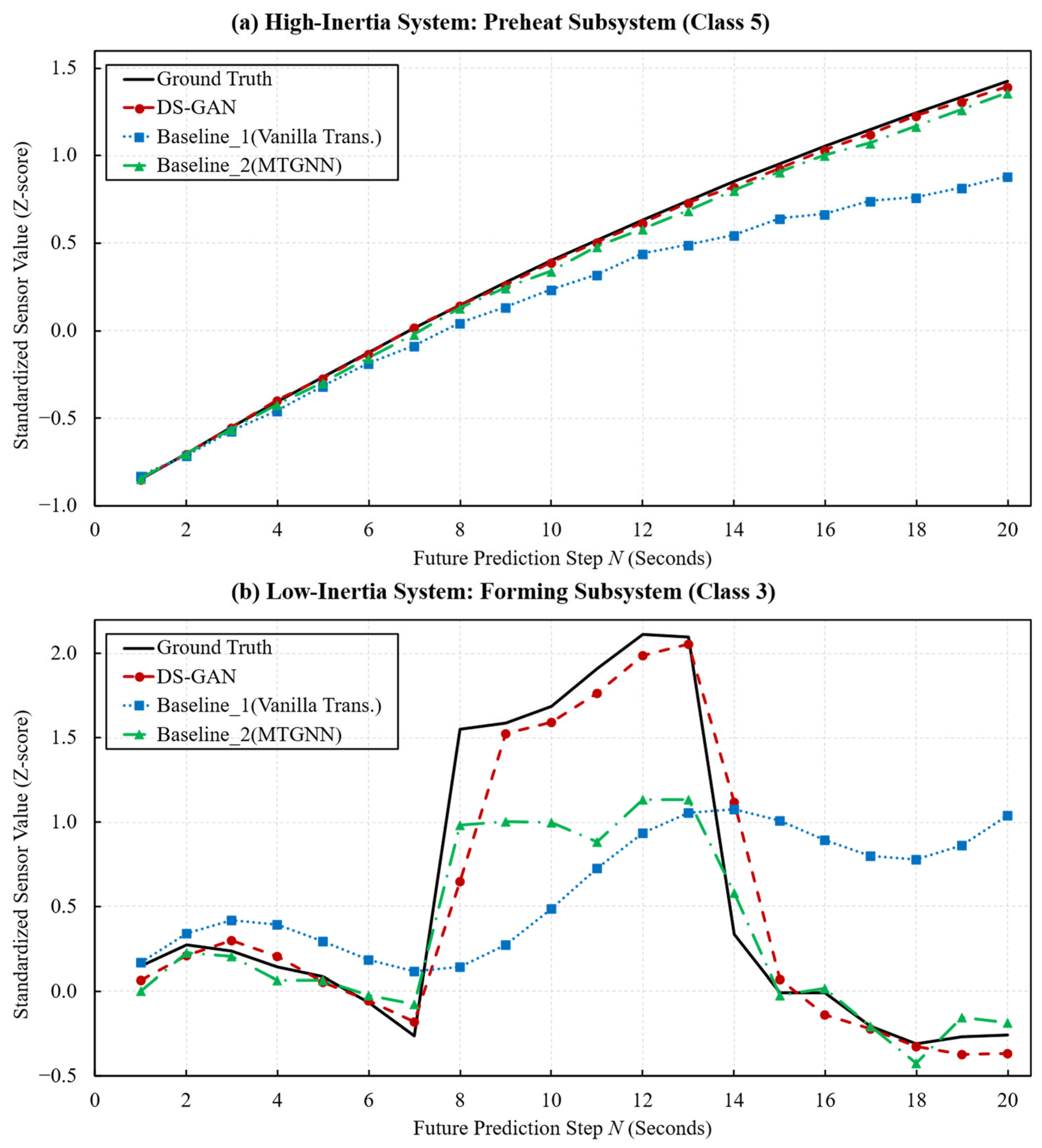
Analyzing the RMSE growth slopes of each subsystem suggests a plausible engineering interpretation: for the evaluated dataset, continuous state prediction errors exhibit a consistent positive correlation with the physical inertia properties of the hardware systems. As shown in Figure 3, high-inertia systems, such as the preheat system, display the strongest anti-decay capabilities, with an RMSE of only 0.028 at N = 20. Because physical responses of these thermal systems possess high continuity, the model can effectively extract smooth low-frequency trends through the historical time window. Conversely, low-inertia systems, such as the forming and optical subsystems, have relatively higher initial RMSE values and steeper growth slopes. These systems involve massive numbers of discrete transient mechanical actions, and the accumulated kinematic uncertainty naturally increases as the prediction step deepens. Nonetheless, the maximum deviation remains strictly bounded below 0.124σ, ensuring feature space integrity for downstream classification.

Figure 3. Diagram of microscopic physical trajectory tracking and topological protection verification.

To systematically ablate the structural necessity of the restricted residual graph evolution mechanism, the trajectory tracking capabilities of Baseline 1 and Baseline 2 were deeply analyzed, as shown in Figure 3. Baseline 1 (Vanilla Transformer) completely lacked spatial topological constraints, flattening all 41-dimensional physical features into independent temporal mappings. Without the ability to capture dynamic thermodynamic and kinetic inter-system coupling, its standardized prediction error diverged nonlinearly after N = 10, completely failing to maintain the basic physical envelope boundary. Baseline 2 (MTGNN) introduced a pure data-driven dynamic graph, which provides short-term spatial alignment capabilities in the initial prediction steps (N ≤ 5). However, without the rigid defense of the static physical prior A_base, its adaptive topology rapidly collapsed under the continuous accumulation of high-frequency industrial noise. As the horizon extended to N = 20, Baseline 2 suffered from severe node over-smoothing and error cascading. In contrast, DS-GAN successfully leveraged the physical inertia coefficient to bind the Macro-RMSE strictly below 0.062, significantly improving the robustness against the vulnerability of pure data-driven models under long-term temporal perturbations on the tested dataset.

4.4. Accuracy Prediction of Future Multi-Subsystem Anomaly Evolution

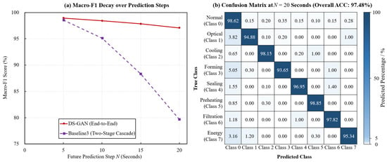
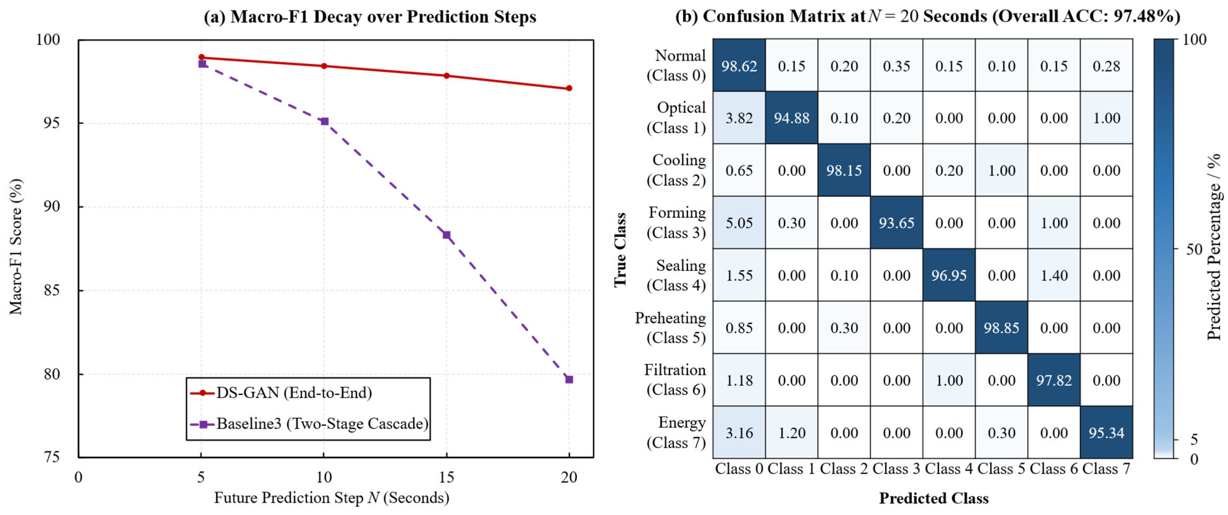
To verify the engineering effectiveness of DS-GAN in long-sequence traceability tasks, this section quantitatively evaluates the global prediction performance and single-class anomaly traceability capabilities of the model. To quantify the severe impact of error cascading on downstream diagnostic tasks, DS-GAN was benchmarked against Baseline 3 (Two-Stage Cascade DS-GAN). In multi-system coupled conditions, Baseline 3 severs the joint backpropagation chain, utilizing a rigid cascade where the regressed trajectories are fed into an offline classifier. As visualized in the decay curves (Figure 4a), while Baseline 3 maintained a Macro-F1 of approximately 98.5% at N = 5, this metric experienced a catastrophic cliff-like drop to 79.6% as the prediction horizon extended to N = 20. This proves that in a decoupled two-stage paradigm, even minor high-frequency deviations in front-end trajectory regression are boundlessly amplified during discrete mapping. By establishing an end-to-end joint inference framework, DS-GAN inherently smooths transient spatial noises along the time axis, demonstrating robust global performance on the validation set (as shown in Table 5).

Figure 4. Decay curves and confusion matrices for macro-anomaly classification.

Table 5. Global prediction performance metrics.

Macro Metrics	Value
Overall Accuracy (ACC)	97.48%
Macro-DR	96.78%
Macro-Precision	97.36%
Macro-F1	97.07%
False Alarm Rate (FAR)	1.85%

The data reveals that the overall accuracy of DS-GAN reaches 97.48%, and the false alarm rate is strictly suppressed to 1.85%. It is crucial to highlight that this predictive performance (Macro-F1 of 97.07%) demonstrates a robust capability for proactive industrial maintenance. This enhancement is fundamentally attributed to the temporal sliding window and multi-task MSE regression acting as a natural denoising filter. Unlike pure spatial diagnosis, which relies heavily on single cross-sections and is highly susceptible to high-frequency industrial noise leading to false positives, DS-GAN smooths these transient noises along the time axis. The introduction of the macroscopic health factor HI effectively filters high-frequency physical overshoots during normal processing, preventing the network from misjudging compliant transient fluctuations as equipment-level degradation. This mechanism significantly reduces the unplanned downtime interventions in actual deployments.

To analyze the decoupling capabilities of the model under concurrent multi-class states, Table 6 details the single-class evolution prediction performance of each physical subsystem.

Table 6. Single-class prediction performance.

Category	Subsystem	Inertial Property	DR (%)	Precision (%)	F1-Score (%)
Class 5	Preheat	High	98.85	99.12	98.98
Class 0	Normal	Stable	98.62	98.95	98.78
Class 2	Cooling	High	98.15	98.54	98.34
Class 6	Filtration	High	97.82	98.26	98.04
Class 4	Sealing	Medium	96.95	97.48	97.21
Class 7	Energy	Low	95.34	96.12	95.73
Class 1	Optical	Low	94.88	95.75	95.31
Class 3	Forming	Low	93.65	94.68	94.16

Table 6 shows that the F1-score of the stable baseline normal state reached 98.78%, indicating no sensitivity drift in the network. For the 7 anomaly categories, the detection rate was stably distributed between 93.65% and 98.85%. This metric distribution proves that the rigid physical grouped projection strategy successfully blocks mapping distortions among multi-physics fields in the latent space. Furthermore, all categories exhibited a slightly higher precision than detection rate (DR), showcasing the model’s design preference for conservative alarming—a critical demand in industrial PHM to control false positive costs.

The magnitude of the metrics strongly reflects the hardware system inertia distribution. High-inertia systems exceed 98% in F1-score, whereas low-inertia systems (e.g., Class 3 Forming, Class 1 Optical), whose fault modes are mostly step-like and lack long-range precursors, inherently face higher uncertainty. Nevertheless, as can be seen from Figure 4, protected by the homoscedastic joint optimization mechanism, the network leverages the smoothed features from the trajectory regression branch to provide a detection rate lower bound of over 93% for these highly dynamic systems.

4.5. Mechanism Validation of Heterogeneous Multi-Task and Homoscedastic Joint Optimization

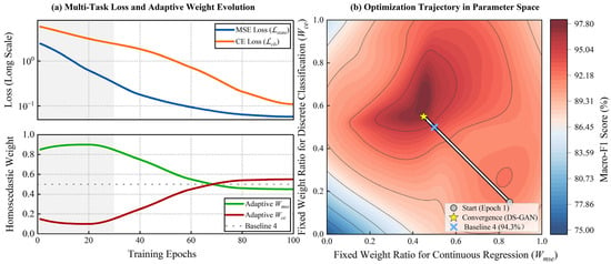
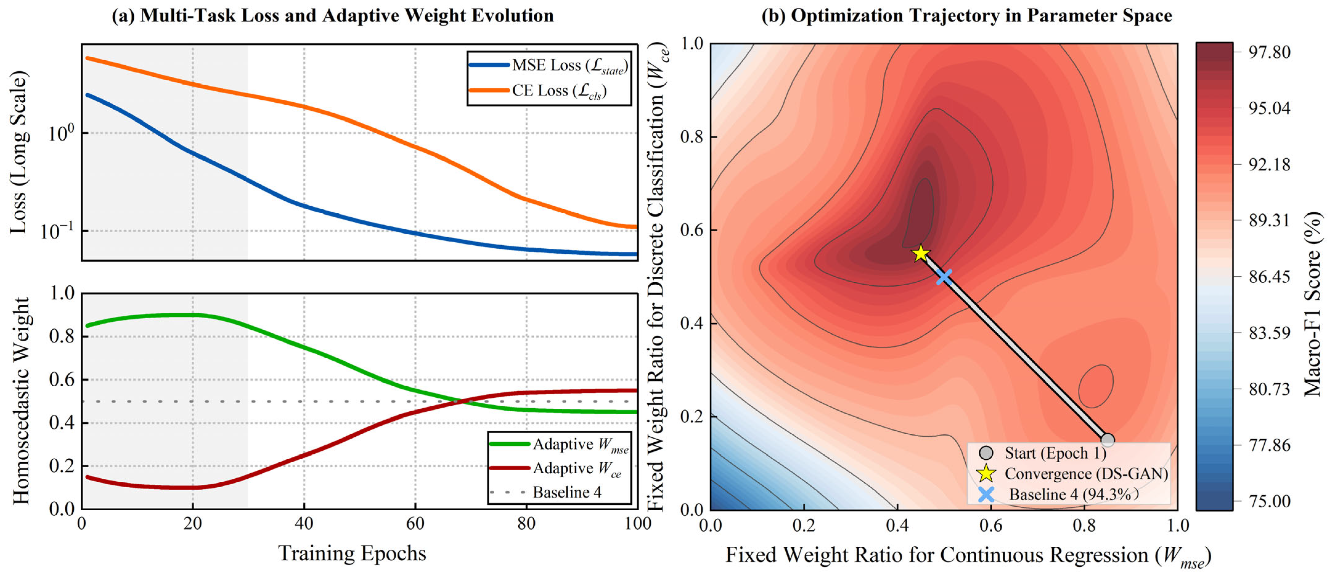
A significant dimensional difference exists between continuous numerical regression and discrete anomaly classification. To verify the effectiveness of the homoscedastic uncertainty loss mechanism, the adaptive weight game process and its optimization trajectory within the parameter space are deconstructed in Figure 5.

Figure 5. Evolutionary plot of homoscedastic multi-task loss and weight dynamics.

In the multi-task learning paradigm, ablation models employing fixed weights easily trigger severe gradient distortion due to the absolute dimensional differences between MSE regression (typically 10⁻¹ to 10⁰) and CE classification (typically 10⁰ to 10¹). As illustrated by the spatial optimization landscape in Figure 5b, Baseline 4 blindly applies a static 1:1 weight ratio (W_mse = 0.5, W_ce = 0.5). This rigid configuration forces the network to become dominated by the classification gradient possessing a larger numerical magnitude, restricting the optimization trajectory to a sub-optimal local minimum with a Macro-F1 score capped at 94.3%. DS-GAN autonomously resolves this dimensional conflict, escaping the fixed-weight trap and achieving a 2.77% peak performance margin over Baseline 4. Conversely, artificially increasing the MSE weight (e.g., W_mse = 0.9, W_ce = 0.1) decreased network sensitivity to low-frequency anomaly features, causing the Macro-F1 to drop to 90.6%. Extreme prioritization of CE loss (e.g., W_mse = 0.1, W_ce = 0.9) similarly degraded the performance to 88.2% due to physical trajectory divergence.

The adaptive strategy introduced in this study defines two learnable log-variance parameters, whose derived dynamic confidence weights are denoted as W_mse and W_ce. Analyzing the evolutionary curves in Figure 5a reveals a curriculum learning mechanism autonomously formed by the network. In the initial defensive stage, due to incompletely aligned long-sequence causal masks, long-term classification tasks harbor extremely high uncertainty. The homoscedastic mechanism senses this difficulty, autonomously suppressing the classification weight and increasing the confidence of continuous trajectory predictions. This phenomenon compels the network to prioritize convergence toward the highly continuous physical sensor evolution baseline. In the later takeover stage, as the fitting of physical continuous states stabilizes, the optimization uncertainty for future discrete classifications decreases. At this point, W_ce smoothly rebounds, shifting the optimization focus toward anomaly boundary delineation.

Crucially, the white optimization trajectory in Figure 5b demonstrates that DS-GAN requires no manual prior weight tuning. Instead, it autonomously navigates the complex hyperparameter space, escaping the rigid constraints of static allocation and ultimately converging at a favourable operating point of (W_mse≈0.45, W_ce≈0.55) observed during training. This mechanism achieved a peak Macro-F1 of 97.07%, ensuring the joint balanced traceability of multiple subsystems across the entire machine.

5. Conclusions

Addressing the critical challenges of strong multi-system physical coupling, variable-length time series inference difficulties, and error cascading induced by multi-task optimization in SLM equipment under continuous printing conditions, this paper proposes a decoupled spatiotemporal graph autoregressive network (DS-GAN). This model successfully achieves continuous trajectory reconstructions and discrete anomaly traceability for future hardware evolution states. First, a joint inference architecture featuring macroscopic–microscopic decoupling and physical topology constraints is constructed. Handling variable-length temporal data spanning extreme ranges, the model decouples high-frequency sequences into independent hardware subsystem representations. Through a degradation gating injection mechanism, it achieves adaptive mapping of macroscopic health factors to microscopic nodes, while the restricted residual graph evolution mechanism anchors the physical reference topology, effectively preventing graph structure collapse under strong noise. Second, the architecture overcomes heterogeneous multi-task dimensional conflicts and long-sequence error cascading bottlenecks.

By introducing homoscedastic uncertainty to construct an adaptive joint loss function, the model forms a curriculum learning mechanism without manual intervention, effectively mitigating gradient conflicts. Quantitative validation shows a Macro-RMSE of only 0.062 at a maximum forward prediction step of 20 s, proving a significant suppressive effect on autoregressive error cascades. Furthermore, the visualized optimization trajectory verifies that the model can autonomously navigate the parameter space to locate a stable solution without relying on rigid static weights.

On complex test sets constrained by the intra-layer truncation protocol, DS-GAN achieved an overall anomaly accuracy of 97.48% and restricted the false alarm rate to 1.85% on the evaluated dataset. In addition, the experimental results on the tested dataset suggest a plausible engineering link between system prediction performance and hardware physical inertia. High-inertia systems (e.g., preheat and cooling) driven by thermodynamics exceed 98% in anomaly detection F1-score. Low-inertia systems (e.g., forming and optical) dominated by transient discrete responses face higher kinematic uncertainty, but their long-range feature capture shortcomings are protected by the homoscedastic game mechanism, securing a detection rate lower bound of over 93%.

References

- Blakey-Milner, B.; Gradl, P.; Snedden, G.; Brooks, M.; Pitot, J.; Lopez, E.; Leary, M.; Berto, F.; du Plessis, A. Metal additive manufacturing in aerospace: A review. Mater. Des. 2021, 209, 110008. [Google Scholar] [CrossRef] [Scilit]
- Taherkhani, K.; Ero, O.; Liravi, F.; Toorandaz, S.; Toyserkani, E. On the application of in-situ monitoring systems and machine learning algorithms for developing quality assurance platforms in laser powder bed fusion: A review. J. Manuf. Process. 2023, 99, 848–897. [Google Scholar] [CrossRef] [Scilit]
- Liu, Q.; Liu, W.; Bian, H.; Xing, F. Decoupled graph attention modeling and anomaly traceability method for multisystem coupling in SLM equipment. Sensors 2026, 26, 3889. [Google Scholar] [CrossRef] [Scilit] [PubMed]
- Ly, S.; Rubenchik, A.M.; Khairallah, S.A.; Guss, G.; Matthews, M.J. Metal vapor micro-jet controls material redistribution in laser powder bed fusion additive manufacturing. Sci. Rep. 2017, 7, 4085. [Google Scholar] [CrossRef] [Scilit] [PubMed]
- Zhang, H.; Vallabh, C.K.P.; Zhao, X. Influence of spattering on in-process layer surface roughness during laser powder bed fusion. J. Manuf. Process. 2023, 104, 289–306. [Google Scholar] [CrossRef] [Scilit]
- Liu, Q.; Liu, W.; Bian, H.; Xing, F. Deep spatiotemporal condition monitoring and subsystem fault classification for selective laser melting equipment. Coatings 2026, 16, 517. [Google Scholar] [CrossRef] [Scilit]
- Jiang, W.; Luo, J. Graph neural network for traffic forecasting: A survey. Expert Syst. Appl. 2022, 207, 117921. [Google Scholar] [CrossRef] [Scilit]
- Rusch, T.K.; Bronstein, M.M.; Mishra, S. A survey on oversmoothing in graph neural networks. arXiv 2023, arXiv:2303.10993. [Google Scholar] [CrossRef] [Scilit]
- Benidis, K.; Rangapuram, S.S.; Flunkert, V.; Wang, Y.; Maddix, D.; Turkmen, C.; Januschowski, T. Deep learning for time series forecasting: Tutorial and literature survey. ACM Comput. Surv. 2022, 55, 1–36. [Google Scholar] [CrossRef] [Scilit]
- Chandra, R.; Goyal, S.; Gupta, R. Evaluation of deep learning models for multi-step ahead time series prediction. IEEE Access 2021, 9, 83105–83123. [Google Scholar] [CrossRef] [Scilit]
- Navon, A.; Shamsian, A.; Fetaya, E.; Chechik, G. Multi-task learning as a bargaining game. In Proceedings of the 39th International Conference on Machine Learning (ICML), Baltimore, MD, USA, 17–23 July 2022; PMLR: Cambridge, MA, USA, 2022; Volume 162, pp. 16428–16446. [Google Scholar] [CrossRef] [Scilit]
- Kirchdorfer, L.; Elich, C.; Kutsche, S.; Stuckenschmidt, H.; Schott, L.; Köhler, J.M. Analytical uncertainty-based loss weighting in multi-task learning. arXiv 2024, arXiv:2408.07985. [Google Scholar] [CrossRef] [Scilit]
- Meng, L.; McWilliams, B.; Jarosinski, W.; Park, H.Y.; Jung, Y.G.; Lee, J.; Zhang, J. Machine learning in additive manufacturing: A review. JOM 2020, 72, 2363–2377. [Google Scholar] [CrossRef] [Scilit]
- Wang, J.; Zhang, X.; Lu, Y. Machine learning in image-based metal additive manufacturing process monitoring and control: A review. Eng. Sci. Addit. Manuf. 2025, 1, 8548. [Google Scholar] [CrossRef] [Scilit]
- Chen, L.; Bi, G.; Yao, X.; Su, J.; Tan, C.; Feng, W.; Benakis, M.; Chew, Y.; Moon, S.K. In-situ process monitoring and adaptive quality enhancement in laser additive manufacturing: A critical review. J. Manuf. Syst. 2024, 74, 527–574. [Google Scholar] [CrossRef] [Scilit]
- Kasilingam, S.; Yang, R.; Singh, S.K.; Wuest, T. Physics-based and data-driven hybrid modeling in manufacturing: A review. Prod. Manuf. Res. 2024, 12, 2305358. [Google Scholar] [CrossRef] [Scilit]
- Wu, Z.; Pan, S.; Long, G.; Jiang, J.; Chang, X.; Zhang, C. Connecting the dots: Multivariate time series forecasting with graph neural networks. In Proceedings of the 26th ACM SIGKDD International Conference on Knowledge Discovery & Data Mining, Virtual Event, 23–27 August 2020; pp. 753–763. [Google Scholar] [CrossRef] [Scilit]
- Bai, L.; Yao, L.; Li, C.; Wang, X.; Wang, C. Adaptive graph convolutional recurrent network for traffic forecasting. Adv. Neural Inf. Process. Syst. 2020, 33, 17804–17815. [Google Scholar] [CrossRef] [Scilit]
- Wu, Z.; Pan, S.; Long, G.; Jiang, J.; Zhang, C. Graph WaveNet for deep spatial-temporal graph modeling. In Proceedings of the 28th International Joint Conference on Artificial Intelligence (IJCAI), Macao, China, 10–16 August 2019; pp. 1907–1913. [Google Scholar] [CrossRef] [Scilit] [PubMed]
- Chen, D.; Lin, Y.; Li, W.; Li, P.; Zhou, J.; Sun, X. Measuring and relieving the over-smoothing problem for graph neural networks from the topological view. Proc. AAAI Conf. Artif. Intell. 2020, 34, 3438–3445. [Google Scholar] [CrossRef] [Scilit]
- Park, M.; Heo, J.; Kim, D. Mitigating oversmoothing through reverse process of GNNs for heterophilic graphs. In Proceedings of the 41st International Conference on Machine Learning (ICML), Vienna, Austria, 21–27 July 2024; PMLR: Vienna, Austria, 2024; Volume 235, pp. 39682–39702. [Google Scholar] [CrossRef] [Scilit]
- Zheng, X.; Wang, Y.; Liu, Y.; Li, M.; Zhang, M.; Jin, D.; Yu, P.S.; Pan, S. Graph neural networks for graphs with heterophily: A survey. IEEE Trans. Knowl. Data Eng. 2026, 38, 4385–4404. [Google Scholar] [CrossRef] [Scilit]
- Zhou, H.; Zhang, S.; Peng, J.; Zhang, S.; Li, J.; Xiong, H.; Zhang, W. Informer: Beyond efficient transformer for long sequence time-series forecasting. Proc. AAAI Conf. Artif. Intell. 2021, 35, 11106–11115. [Google Scholar] [CrossRef] [Scilit]
- Nie, Y.; Nguyen, N.H.; Sinthong, P.; Kalagnanam, J. A time series is worth 64 words: Long-term forecasting with transformers. In Proceedings of the International Conference on Learning Representations (ICLR), Kigali, Rwanda, 1–5 May 2023. [Google Scholar] [CrossRef] [Scilit]
- Mao, Y.; Zhong, S.; Yin, H. Model-based deep reinforcement learning for active control of flow around a circular cylinder using action-informed episode-based neural ordinary differential equations. Phys. Fluids 2024, 36, 087158. [Google Scholar] [CrossRef] [Scilit]
- Liu, B. From Diversity to Adaptivity: Effective Multitask Learning and Continual Learning Neural Architectures. Ph.D. Thesis, The University of Texas at Austin, Austin, TX, USA, 2025. [Google Scholar] [CrossRef]
- Senushkin, D.; Patakin, N.; Kuznetsov, A.; Konushin, A. Independent component alignment for multi-task learning. In Proceedings of the IEEE/CVF Conference on Computer Vision and Pattern Recognition (CVPR), Vancouver, BC, Canada, 18–22 June 2023; pp. 20083–20093. [Google Scholar] [CrossRef] [Scilit]
- Kendall, A.; Gal, Y.; Cipolla, R. Multi-task learning using uncertainty to weigh losses for scene geometry and semantics. In Proceedings of the IEEE Conference on Computer Vision and Pattern Recognition (CVPR), Salt Lake City, UT, USA, 18–23 June 2018; pp. 7482–7491. [Google Scholar] [CrossRef] [Scilit]
Disclaimer/Publisher’s Note: The statements, opinions and data contained in all publications are solely those of the individual author(s) and contributor(s) and not of MDPI and/or the editor(s). MDPI and/or the editor(s) disclaim responsibility for any injury to people or property resulting from any ideas, methods, instructions or products referred to in the content. |
© 2026 by the authors. Licensee MDPI, Basel, Switzerland. This article is an open access article distributed under the terms and conditions of the Creative Commons Attribution (CC BY) license.