Abundance-Weighted Carbon-Isotope Mixing in Natural Gas: Nonlinear Trajectories and Implications for Source Interpretation

Abstract

Carbon isotope trends of light hydrocarbons in mature to overmature natural gases are commonly evaluated against gas wetness ([C₂ + C₃]/[C₁ + C₂ + C₃]), yet the geometric effects of component-specific abundance contrasts are often conflated with reaction- or transport-driven fractionation. We develop an abundance-weighted framework for binary mixing that conserves ¹²C and ¹³C and relates the bulk mixing fraction x to a component-specific effective coordinate, ω_i(x) = x/[x + (1 − x)ρ_i], where ρ_i is the abundance ratio of component i in the endmembers. Thus, δ¹³C_i is linear in ω_i but generally nonlinear in x when ρ_i ≠ 1. Analytical expressions and C₁–C₃ benchmark simulations show that the “linear interpolation bias” is controlled jointly by isotopic contrast and abundance asymmetry, producing component-specific curvature of δ¹³C_i isotope vs. wetness trends. Binary mixing of fixed endmembers cannot produce a true rollover in an individual hydrocarbon isotope trajectory, although isotope-contrast metrics may develop local extrema because different components follow different effective mixing coordinates. Reparameterizing the trajectories by wetness can shift and nonlinearly compress or stretch pre-existing features along the horizontal axis, but it cannot create new extrema or change their amplitudes. The proposed framework therefore provides a mass-balance null model for evaluating mixing interpretations and identifying cases that require evolving endmembers, multistage charging, reaction, or transport fractionation.

1. Introduction

Stable carbon isotopes of light hydrocarbons, principally methane, ethane, and propane, are widely used to classify the origin, assess the thermal maturity, and evaluate migration and mixing of natural gases. Interpretations can be enhanced by integrating isotope data with molecular composition (e.g., C₂₊ abundance) and, where available, hydrogen isotopes and other geochemical tracers [1,2,3]. These frameworks are widely used interpretive tools for distinguishing microbial and thermogenic gases and for tracking progressive thermal evolution [2]. Nevertheless, datasets from low-permeability reservoirs and late-mature to overmature systems commonly depart from simple monotonic isotope (δ ¹³C …) maturity trends [4,5,6,7,8].

A recurring feature is the greater dispersion and stronger apparent nonlinearity of ethane and propane carbon isotope ratio trends relative to methane over comparable compositional ranges. In shale, tight, and deep-basin gases, δ¹³C₂ and δ¹³C₃ may depart from expected maturity trends, and components can become isotopically “lighter” toward very “dry” conditions, whereas δ¹³C₁ often remains comparatively systematic [4,7,8,9,10]. Similar behavior has also been reported in conventional reservoirs affected by high maturity and complex charging histories, showing that the problem is not restricted to a single reservoir type [7,8].

Proposed explanations include secondary cracking and mixing of primary and secondary products, redox-related Rayleigh fractionation, diffusive or advective transport, desorption, and water- or mineral-mediated reactions that preferentially affect C₂–C₃ hydrocarbons [5,7,11,12,13,14,15,16]. These mechanisms are physically plausible and are supported by field, experimental, and kinetic evidence [8,17,18]. These mechanisms are also not mutually exclusive. Wetness is a derived, rather than independent, variable in the mixing model because it is calculated from the same component abundances that vary with the underlying bulk-gas mixing fraction x. Thus, curvature in isotope-wetness space reflects the joint dependence of isotope composition and wetness on the underlying mixing state and is not uniquely diagnostic of mechanism. A defensible interpretation should therefore begin with the trajectories permitted by closed-system mass balance.

Previous studies have established the mass-balance basis of nonlinear and abundance-weighted isotope mixing. Langmuir et al. [19] derived the general nonlinear mixing relation for ratio variables, whereas Berner and Faber [20] applied concentration-weighted carbon-isotope mixing to methane, ethane, and propane. Xia et al. [21] further showed that mixing of natural gases from different sources can result in substantial changes in the relative order of isotope composition of hydrocarbon components, potentially altering conventional genetic interpretations. Thus, abundance-weighted isotope mixing itself is not new. What remains less explicit is how molecular-abundance asymmetry of the source gases controls component-specific trajectories and interpolation bias, how different hydrocarbon trends become divergent within a common mixing process, and whether and which apparent reversals can arise from fixed-endmember binary mixing.

Building on this foundation, we develop an analytical and diagnostic formulation of the fixed-endmember binary-mixing problem. We begin from an exact isotope-ratio mass balance and its practical delta approximation, and introduce a component-specific abundance ratio, a normalized asymmetry parameter, and an effective mixing coordinate. These parameters are used to quantify the bias introduced by bulk-fraction linear interpolation, i.e., by approximating δ¹³C_i(x) as xδ¹³C_i,A + (1-x)δ¹³C_i,B rather than accounting for component-specific abundances, including the maximum magnitude and location of this bias. We then formulate a coupled C₁–C₃ system in which all components share a common bulk-gas mixing fraction, distinguish non-monotonic isotope-contrast behavior from true rollover of an individual hydrocarbon-isotope trajectory, and examine how these relationships are reparametrized in wetness space.

The framework is deliberately formulated for a closed, binary, fixed-endmember model. It is not intended to replace kinetic, reaction, or transport models. Instead, it provides a testable mass-balance null model that defines the behavior permitted by mixing alone. Fixed-endmember binary mixing can generate component-specific curvature, cross-component nonlinearity, and extrema in isotope-contrast metrics, but it cannot generate a true rollover of an individual δ¹³C_i trajectory. Observations that violate these constraints, or that require geologically implausible endmember compositions, indicate where additional endmembers, evolving source compositions, multistage charging, reaction, or transport fractionation must be considered.

2. Theoretical Framework and Model Formulation

2.1. Binary Isotopic Mixing Under Mass-Balance Constraints

For a given hydrocarbon component i, physical mixing conserves the inventories of ¹²C and ¹³C carried by that component; the isotope ratio itself is not additive. We therefore begin with an exact isotope-ratio mass balance and then derive the practical delta-form used in the simulations.

Let R_i,A = N_13,iA/N_12,i,A and R_iB = N_13,iB/N_12,i,B be the carbon-isotope ratios of component i in endmembers A and B. Let x be the bulk-gas mixing fraction of endmember A, with (1 − x) contributed by endmember B. Let n_i,A and n_i,B denote the abundance of component i per unit amount of the corresponding endmember, normally its mole fraction; any proportional abundance measure is equivalent. The products xn_i,A and (1 − x)n_i,B are therefore the amounts of component i delivered to the mixture. Because R = N₁₃/N₁₂, partitioning component carbon between the two isotopes gives

$$N_{12,i,A}\propto {\displaystyle \frac{n_{i,A}}{1+R_{i,A}}}, N_{13,\mathit{iA}}\propto {\displaystyle \frac{n_{\mathit{iA}}{R}_{i,A}}{1+R_{i,A}}}$$

(1)

$$N_{12,i,B}\propto {\displaystyle \frac{n_{i,B}}{1+R_{i,B}}}, N_{13,\mathit{iB}}\propto {\displaystyle \frac{n_{i,B}{R}_{i,B}}{1+R_{i,B}}}$$

(2)

The isotope inventories of mixtures are additive. Thus, for a binary mixture:

N_12,i,mix = xN_12,i,A + (1 − x)N_12,i,B,N_13,i,mix = xN_13,i,A + (1 − x)N_13,i,B

(3)

Substitution into Equation (3) gives the exact isotope ratio of the mixture:

$$R_{i,\mathit{mix}}\left(x\right)={\displaystyle \frac{N_{13,i,\mathit{mix}}}{N_{12,i,\mathit{mix}}}}={\displaystyle \frac{x{n}_{i,A}\frac{R_{i,A}}{1+R_{i,A}}+\left(1-x\right)n_{i,B}\frac{R_{i,B}}{1+R_{i,B}}}{x{n}_{i,A}\frac{1}{1+R_{i,A}}+\left(1-x\right)n_{i,B}\frac{1}{1+R_{i,B}}}}$$

(4)

Carbon-isotope compositions are conventionally reported in delta notation relative to VPDB:

$${\mathit{\delta }}^{13}{C}_i=1000\times \left({\displaystyle \frac{R_i}{R_{\mathit{VPDB}}}}-1\right)$$

(5)

where R_i denotes the isotope ratio of component i. For the carbon-isotope ratios relevant to natural gas, the approximation 1 + R_i ≈ 1 introduces only a very small error. Direct comparison of the exact isotope-ratio mass balance with the practical delta approximation gives

$$0\ll {\mathit{\delta }}^{13}{C}_{i,\mathit{approx}}-{\mathit{\delta }}^{13}{C}_{i,\mathit{exact}}\le {\displaystyle \frac{R_{\mathit{VPDB}}}{4000}}{\left({\mathit{\delta }}^{13}{C}_{i,A}-{\mathit{\delta }}^{13}{C}_{i,B}\right)}^2$$

where delta values are expressed in %. For the largest component-specific endmember isotope contrast used in Table 1, 25%, and R_VPDB ≈ 0.0112, the resulting error is less than 0.0018%. This is several orders of magnitude smaller than the abundance-controlled effects considered below. Equation (4) then reduces to the following practical delta-form:

$${\mathit{\delta }}^{13}{C}_i\left(x\right)\approx {\displaystyle \frac{x{n}_{i,A}{\mathit{\delta }}^{13}{C}_{i,A}+\left(1-x\right)n_{i,B}{\mathit{\delta }}^{13}{C}_{i,B}}{x{n}_{i,A}+\left(1-x\right)n_{i,B}}}$$

(6)

Table 1. Representative endmember configurations for coupled C₁–C₃ mixing simulations. Except for U1, C₁–C₃ mole fractions are normalized to unity within each endmember; U1 is defined on a common bulk-gas molar basis to illustrate unequal hydrocarbon totals. In U1, endmember A contains 40% non-hydrocarbon gas and therefore has a total C₁–C₃ abundance of 0.60, whereas endmember B has a C₁–C₃ total of 1.00. δ¹³C values are in ‰ VPDB.

Case	Purpose	Endmember A (C1, C2, C3)	δ13CA (C1, C2, C3)	Endmember B (C1, C2, C3)	δ13CB (C1, C2, C3)	Approx. k1/k2/k3
T1	Typical symmetric	(0.90,0.07,0.03)	(−42, −30, −28)	(0.90, 0.07, 0.03)	(−32, −24, −22)	0.50/0.50/0.50
T2	Typical asymmetric	(0.95,0.04,0.01)	(−40, −29, −27)	(0.80, 0.12, 0.08)	(−34, −26, −24)	0.54/0.25/0.11
E1	Extreme dry–wet	(0.98,0.015,0.005)	(−38, −27, −25)	(0.70, 0.18, 0.12)	(−45, −32, −30)	0.58/0.08/0.04
G1	Geometric trap (small Δδ)	(0.97,0.02,0.01)	(−36, −28, −26)	(0.78, 0.14, 0.08)	(−34, −27, −25)	0.55/0.13/0.11
M1	Decoupled: k1 ≫ k2, k3	(0.995,0.004,0.001)	(−60, −35, −33)	(0.85, 0.10, 0.05)	(−40, −28, −26)	0.54/0.04/0.02
M2	Decoupled: k1 < k2, k3	(0.85,0.10,0.05)	(−44, −30, −28)	(0.995, 0.004, 0.001)	(−48, −33, −31)	0.46/0.96/0.98
S1	Screening failure (δ overlap)	(0.98,0.015,0.005)	(−41, −29, −27)	(0.78, 0.14, 0.08)	(−42, −30, −28)	0.56/0.10/0.06
S2	Linear-safe control	(0.90,0.07,0.03)	(−55, −40, −38)	(0.90, 0.07, 0.03)	(−30, −22, −20)	0.50/0.50/0.50
U1	Unequal hydrocarbon totals	(0.597,0.0024,0.0006)	(−60, −35, −33)	(0.85, 0.1, 0.05)	(−40, −28, −26)	0.41/0.02/0.01

This form has been applied to gaseous hydrocarbons and to gas-source discrimination indices [20,21]. In Equations (4) and (6), the weights xn_i,A and (1 − x)n_i,B make explicit that isotope mixing is component-specific: the bulk-gas mixing fraction x and (1 − x) are not generally the fractions of component i derived from endmembers A and B, respectively.

Equation (6) is often replaced by a linear interpolation of delta values:

δ¹³C_i,linear(x) = xδ¹³C_i,A + (1 − x)δ¹³C_i,B

(7)

Here the influence of the difference in abundances of isotope species (n_i,A and n_i,B) in the endmember components (A and B) is ignored. Equation (7) is only exact when n_i,A = n_i,B, or equivalently when the component-specific contribution follows the bulk mixing fraction.

2.2. Parameterization of Endmember Abundance Asymmetry

Equation (6) shows that the isotope composition of component i is controlled by the relative amount of that component supplied by the two endmembers, not by x alone. Its denominator, xn_i,A + (1 − x)n_i,B, is the total amount of component i in the mixture.

We therefore define the effective mixing coordinate for component i as

$${\omega }_i\left(x\right)\equiv {\displaystyle \frac{x{n}_{i,A}}{x{n}_{i,A}+\left(1-x\right)n_{i,B}}}$$

(8)

This quantity is the fraction of component i in the mixture supplied by endmember A. Equation (6) can then be written as

δ¹³C_i(x) = ω_i(x)δ¹³C_i,A + [1 − ω_i(x)]δ¹³C_i,B

(9)

Equation (9) is affine (linear) in ω_i but generally nonlinear in x. Whenever n_i,A ≠ n_i,B, ω_i(x) departs from x and produces abundance-controlled curvature in δ¹³C_i(x).

To isolate this control, we define the endmember abundance ratio

$${\rho }_i\equiv {\displaystyle \frac{n_{i,B}}{n_{i,A}}}$$

(10)

which compares the abundance of component i in endmember B with that in endmember A. Substitution into Equation (8) gives

$${\omega }_i\left(x\right)={\displaystyle \frac{x}{x+\left(1-x\right){\rho }_i}}$$

(11)

For fixed isotopic endmembers, the shape of the effective coordinate is governed by ρ_i. When ρ_i = 1, ω_i = x and Equation (9) reduces to linear interpolation. As ρ_i departs from unity, ω_i(x) increasingly differs from x, producing stronger curvature in the isotope trajectory. The absolute deviation in delta units, however, also scales with the isotope contrast between the endmembers. Importantly, such curvature does not imply non-monotonicity. Combining Equations (9) and (11) and differentiating with respect to x gives

$${\displaystyle \frac{d{\mathit{\delta }}^{13}{C}_i}{\mathit{dx}}}=({\mathit{\delta }}^{13}{C}_{i,A}-{\mathit{\delta }}^{13}{C}_{i,B}){\displaystyle \frac{{\rho }_i}{{\left[x+(1-x){\rho }_i\right]}^2}}$$

For positive component abundances, ρ_i > 0, and the denominator is positive throughout 0 ≤ x ≤ 1. Therefore, whenever the two isotopic endmembers differ, the derivative has a constant sign and δ¹³C_i(x) is strictly monotonic. Fixed-endmember binary mixing can thus produce curvature in an individual-component trajectory, but it cannot produce a true rollover.

For visualization, the unbounded ratio ρ_i ∈ (0,∞) is replaced by the parameter k_i:

$$k_i\equiv {\displaystyle \frac{1}{1+{\rho }_i}}={\displaystyle \frac{n_{i,A}}{n_{i,A}+n_{i,B}}}$$

(12)

This parameter ranges from 0 to 1 and represents the share of species i in the endmember A relative to the sum of this species in both endmembers (n_i,A + n_i,B). Note that it is not the contribution of A to a given mixture. We use ρ_i in the derivations and k_i in the figures.

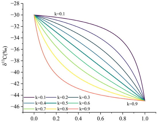
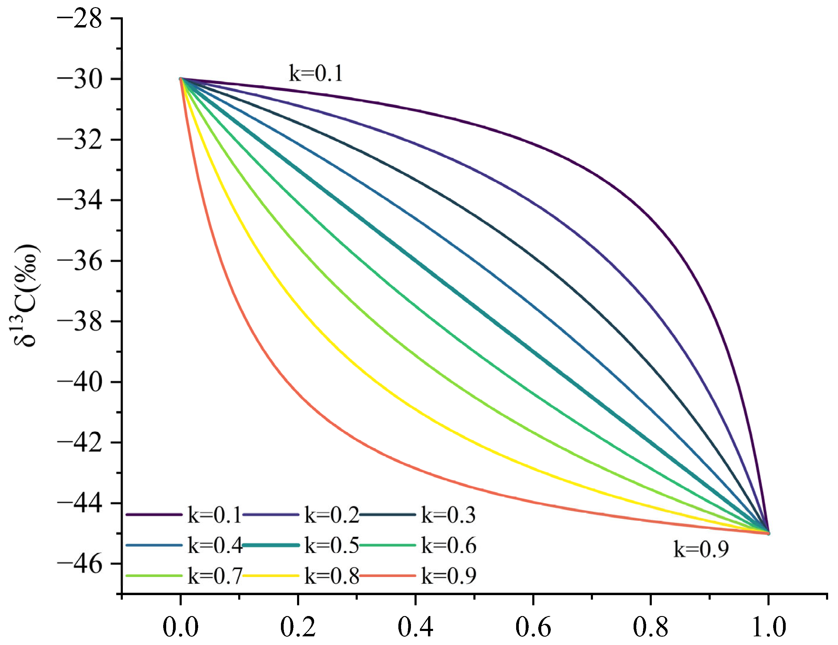
Figure 1 illustrates this effect for fixed-endmember isotope compositions of δ¹³C_A = −45‰ and δ¹³C_B = −30‰. For k_i = 0.5 (ρ_i = 1; equal amounts of species i in both endmembers), the trajectory is linear in x. As k_i approaches 0 or 1, the effective coordinate becomes increasingly asymmetric, and the trajectory becomes more curved. The normalized trajectory shape is controlled by k_i, whereas the magnitude of the deviation in ‰ scales with the endmember isotope contrast. Thus, k_i indicates the potential failure of linear interpolation, but abundance asymmetry and isotope contrast jointly determine whether the bias is observable.

Figure 1. Effect of the abundance asymmetry on the carbon-isotope mixing trajectory of a specific component (C₁, C₂, C₃, …). The calculated δ¹³C_i values for the mixture are plotted against the proportion of endmember A in the mixture. Isotopic compositions of the carbon species of the endmembers are −45‰ (δ¹³C_i,A) and −30‰ (δ¹³C_i,B), respectively. Trajectories were calculated for k_i values from 0.1 to 0.9. The trajectory is linear at k_i = 0.5 (ρ_i = 1) and becomes progressively more curved as k_i approaches 0 or 1.

2.3. Bias Introduced by Bulk-Fraction Linear Interpolation

The deviation between the abundance-weighted trajectory (Equation (6)) and linear interpolation (Equation (7)) is defined as

Δδ_i(x,ρ_i) = δ¹³C_i,abundance(x) − δ¹³C_i,linear(x)

(13)

By this definition, Δδ_i > 0 means that linear interpolation underestimates the abundance-weighted δ¹³C_i value, whereas Δδ_i < 0 means that it overestimates it. For the typically negative δ¹³C values of natural gas, underestimation corresponds to predicting a more negative numerical value.

Substitution of Equations (6) and (7) gives

$$\Delta {\mathit{\delta }}_i\left(x, {\rho }_i\right)=\left({\mathit{\delta }}^{13}{C}_{i,A}-{\mathit{\delta }}^{13}{C}_{i,B}\right)\left[{\displaystyle \frac{x}{x+\left(1-x\right){\rho }_i}}-x\right]$$

(14)

Equation (14) is a closed-form expression for the systematic bias. Substituting k_i = 1/(1 + ρ_i) gives

$$\Delta {\mathit{\delta }}_i\left(x, k_i\right)=\left({\mathit{\delta }}^{13}{C}_{i,A}-{\mathit{\delta }}^{13}{C}_{i,B}\right)\left[{\displaystyle \frac{x}{x+\left(1-x\right)\left(\frac{1}{k_i}-1\right)}}-x\right]$$

(15)

The sign of the bias depends jointly on the isotope ordering of the endmembers and the abundance asymmetry. For 0 < x < 1,

sgn(Δδ_i) = sgn[(δ¹³C_i,A − δ¹³C_i,B)(1 − ρ_i)]

Thus, abundance asymmetry alone does not determine the sign of the bias; the isotope ordering of the endmembers must also be considered.

The location and magnitude of the maximum interpolation bias can also be obtained analytically. For ρ_i > 0, ρ_i ≠ 1, and a nonzero endmember isotope contrast, differentiating Equation (14) with respect to x gives a single interior extremum at

$$x_{\mathit{max}}({\rho }_i)={\displaystyle \frac{\sqrt{{\rho }_i}}{1+\sqrt{{\rho }_i}}}$$

(16)

Substitution of x_max(ρ_i) into Equation (14) gives the signed extremum

$${\Delta \mathit{\delta }}_i(x_{\mathit{max}},{\rho }_i)=({\mathit{\delta }}^{13}{C}_{i,A}-{\mathit{\delta }}^{13}{C}_{i,B}){\displaystyle \frac{1-\sqrt{{\rho }_i}}{1+\sqrt{{\rho }_i}}}$$

(17)

and hence the maximum absolute bias over the binary-mixing interval is

$$\underset{0\le x\le 1}{\max }\left|\Delta {\mathit{\delta }}_i(x,{\rho }_i)\right|=\left|{\mathit{\delta }}^{13}{C}_{i,A}-{\mathit{\delta }}^{13}{C}_{i,B}\right|{\displaystyle \frac{\left|1-\sqrt{{\rho }_i}\right|}{1+\sqrt{{\rho }_i}}}$$

(18)

Thus, abundance asymmetry controls both the location and the normalized magnitude of the maximum interpolation bias, whereas the endmember isotope contrast scales its absolute magnitude. When ρ_i = 1 (k_i = 0.5), or when the two isotopic endmembers are identical, the bias is zero throughout the mixing interval.

Equation (18) therefore provides a practical criterion for evaluating whether linear interpolation is adequate for a given application. When the predicted maximum absolute bias is smaller than the acceptable error tolerance, the linear approximation remains within that tolerance throughout the binary-mixing interval. Larger predicted biases indicate that deviations from linear interpolation may be resolvable, subject to sampling coverage and analytical and endmember uncertainties.

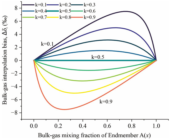
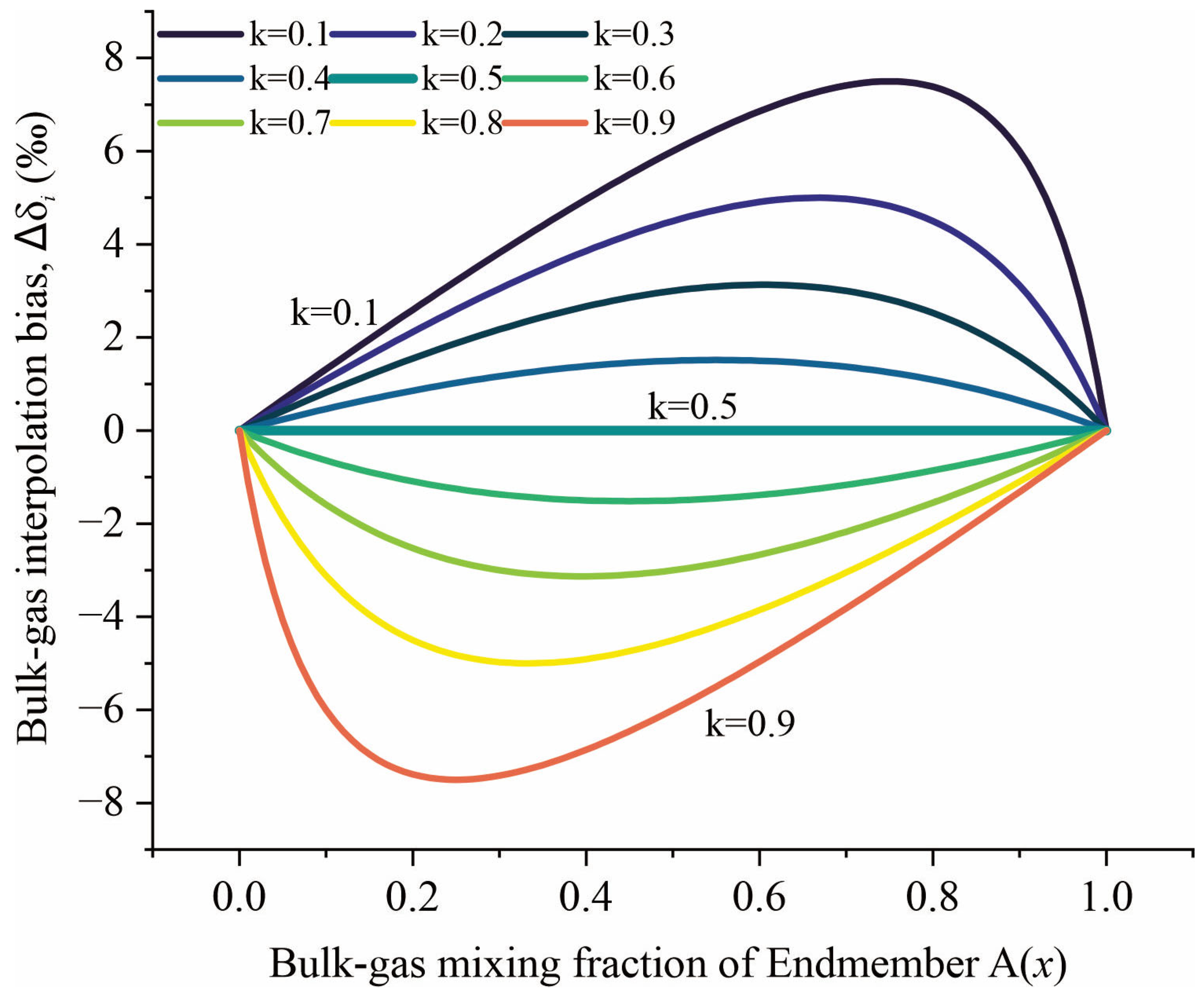
Figure 2 illustrates these analytical results for the fixed isotope contrast used in Figure 1. The bias is zero at x = 0 and x = 1, where the mixture is a pure endmember, and is identically zero for k_i = 0.5 (ρ_i = 1). For asymmetric endmembers, the absolute bias reaches its maximum at the mixing fraction given by Equation (16). For example, k_i = 0.1 and 0.9 correspond to ρ_i = 9 and 1/9, respectively, giving x_max = 0.75 and 0.25. For the 15‰ endmember isotope contrast used in Figure 2, Equation (18) predicts a maximum absolute bias of 7.5‰ in both cases, consistent with the plotted extrema.

Figure 2. Bulk-gas interpolation bias, Δδ_i, as a function of bulk-gas mixing fraction x for different values of the normalized abundance parameter k_i. The bias is defined as Δδ_i = δ¹³C_i,abundance − δ¹³C_i,linear. Curves correspond to k_i = 0.1–0.9 for fixed-endmember isotope compositions of δ¹³C_i,A = −45‰ and δ¹³C_i,B = −30‰. Positive Δδ_i indicates that linear interpolation underestimates the abundance-weighted isotope value, whereas negative Δδ_i indicates that it overestimates it. The bias is zero at the pure endmembers and for k_i = 0.5, and its maximum absolute magnitude and location are given by Equations (16)–(18).

For the isotope ordering used in Figure 2, δ¹³C_A < δ¹³C_B. Therefore, k_i < 0.5 (ρ_i > 1) gives Δδ_i > 0, meaning that linear interpolation underestimates the abundance-weighted isotope value, whereas k_i > 0.5 (ρ_i < 1) gives Δδ_i < 0, meaning that it overestimates it. The sign would reverse if the isotope ordering of the two endmembers were reversed. Linear interpolation therefore introduces a predictable, component-specific bias rather than random uncertainty. Equations (16)–(18) provide a direct basis for evaluating the location, magnitude, and practical significance of the interpolation bias for any specified endmember pair.

3. Coupled C₁–C₃ Mixing and Joint Constraints

The single-component derivation applies separately to methane, ethane, and propane. Because these components are commonly measured together, they can provide complementary constraints on gas origin and mixing [21,22,23,24,25,26].

For each component in a binary mixture,

$${\mathit{\delta }}^{13}{C}_i\left(x\right)={\mathit{\delta }}^{13}{C}_{i,B}+{\displaystyle \frac{x\left({\mathit{\delta }}^{13}{C}_{i,A}-{\mathit{\delta }}^{13}{C}_{i,B}\right)}{x+\left(1-x\right){\rho }_i}}, i\in \left\{1,2,3\right\}$$

(19)

where ρ_i = n_i,B/n_i,A is component-specific. Equation (19) applies to i = 1,2,3 with all three components sharing the same bulk-gas mixing fraction x but having component-specific ρ_i values and isotope endpoints.

If the endmember isotope compositions and molecular abundances are known, each observed hydrocarbon isotope composition provides a component-specific isotope-derived estimate, ${\widehat{x}}_{i,\mathit{iso}}$ of the same physical bulk-gas mixing fraction x. For a noise-free observation that is exactly consistent with the specific fixed-endmember model, ${\widehat{x}}_{1,\mathit{iso}}={\widehat{x}}_{2,\mathit{iso}}={\widehat{x}}_{3,\mathit{iso}}=x$. For real observations, analytical uncertainty and model inconsistency may cause the three component-specific estimates to differ. Their agreement therefore provides a diagnostic test of whether the specified endmembers and abundance ratios are compatible with a common physical mixing fraction. For observed isotope compositions, a joint isotope-derived estimate of the bulk-gas mixing fraction is obtained by minimizing an uncertainty-weighted cross-component objective function

$$\mathsf{\Phi }\left(x\right)={\displaystyle {\sum }_{i=1}^3}{\left[{\displaystyle \frac{{\mathit{\delta }}^{13}{C}_{i,\mathit{obs}}-{\mathit{\delta }}^{13}{C}_i(x)}{{\sigma }_{i,\mathit{eff}}(x)}}\right]}^2$$

(20)

where δ¹³C_i,obs is the observed isotope composition of component i, δ¹³C_i(x) is the abundance-weighted prediction from Equation (9), and σ_i,eff(x) is the effective uncertainty associated with the corresponding isotope residual. Assuming independent uncertainties in the observed isotope composition and the two endmember isotope compositions, the effective variance was approximated as

$${\sigma }_{i,\mathit{eff}}^2\left(x\right)={\sigma }_{i,\mathit{obs}}^2+{\omega }_i{\left(x\right)}^2{\sigma }_{i,A}^2+{\left[1-{\omega }_i\left(x\right)\right]}^2{\sigma }_{i,B}^2$$

(21)

where σ_i,obs, σ_i,A, and σ_i,B denote the isotope uncertainties of the observation, endmember A, and endmember B, respectively. Because ω_i(x) is component-specific, the effective uncertainty can also vary among C₁, C₂, and C₃ and with the trial mixing fraction x.

The joint isotope-derived estimate of the bulk-gas mixing fraction is then

$${\widehat{x}}_{\mathit{iso}}=\underset{0\le x\le 1}{\mathrm{a}\mathit{rg}\min }\mathsf{\Phi }\left(x\right)$$

(22)

Thus, $\mathsf{\Phi }\left({\widehat{x}}_{\mathit{iso}}\right)$ represents the minimum uncertainty-weighted misfit among the C₁–C₃ isotope observations for a specified pair of fixed endmembers.

For known endmember parameters and noise-free observations that are exactly consistent with the model, the bulk-gas mixing fraction x is uniquely determined provided that at least one component has distinct endmember isotope compositions. This follows from the strict monotonicity of that component-specific mapping. For noisy observations, or when the different components are not mutually consistent with a single value of x, however, monotonicity of the individual mappings does not by itself guarantee a unique minimum of the joint least-squares objective. The objective function should therefore be evaluated over the admissible interval 0 ≤ x ≤ 1, and the resulting estimate, ${\widehat{x}}_{\mathit{iso}}$, its uncertainty, and any competing minima should be reported. In applications, analytical uncertainties should be used as weights and uncertainty in endmember parameters should be propagated. Accordingly, the coupled formulation is best viewed as an internal-consistency test rather than as a guarantee of a uniquely identifiable least-squares solution. Agreement among components supports the specified endmembers and abundance ratios; disagreement may reflect incorrect endmembers, unmodeled processes, or weak identifiability rather than mixing alone.

4. Benchmark Simulations and Results

We use synthetic binary endmember configurations to isolate the geometric consequences of molecular-abundance asymmetry and cross-component coupling. The simulations are diagnostic rather than basin-calibrated: they define expected behavior under controlled assumptions and provide a reference for evaluating field data.

4.1. Design of Representative Endmember Configurations

Endmember pairs were designed along three axes: (1) isotope contrast, ranging from nearly overlapping values (1–3‰) to differences greater than 20‰; (2) component-specific abundance asymmetry, represented by k₁, k₂, and k₃; and (3) cross-component coupling, represented by the similarity or divergence among those parameters.

For the normalized benchmark configurations T1–S2, the C₁–C₃ sum to unity within each endmember, ∑_i n_i,A = ∑_i n_i,B = 1. This normalization facilitates comparison but also imposes a compositional-closure constraint on the abundance ratios. Since ρ_i = n_i,B/n_i,A (Equation (10)), $\mathbf{\sum }_i{n}_{i,A}{\rho }_i=\mathbf{\sum }_i{n}_{i,B}=1$.

Thus, the n_i,A–weighted mean of ρ_i is unity, and ρ₁, ρ₂ and ρ₃ are not independent. For positive component abundances, they cannot all exceed unity or all be below unity unless ρ₁ = ρ₂ = ρ₃ = 1. Equivalently, except for the fully symmetric case, the corresponding k_i values cannot all lie on the same side of 0.5. This closure constraint limits the combinations of component asymmetry that can occur in the normalized benchmark set.

The normalized configurations also have H_A = H_B = 1, making wetness a linear function of the physical mixing fraction x. To examine the unequal-total case, configuration U1 is defined on a common bulk-gas molar basis with H_A = 0.60 and H_B = 1.00. U1 is used specifically to illustrate the nonlinear mapping between x and wetness discussed in Section 6.

Table 1 includes a symmetric reference (T1), moderately and extremely asymmetric cases (T2 and E1), a low-isotope-contrast asymmetric case (G1), two oppositely decoupled cases (M1 and M2), diagnostic controls (S1 and S2), and the unequal-total configuration U1. These configurations span representative mixing geometries without implying that they exhaust the range of natural-gas compositions.

4.2. Component-Specific Isotopic Mixing Trajectories

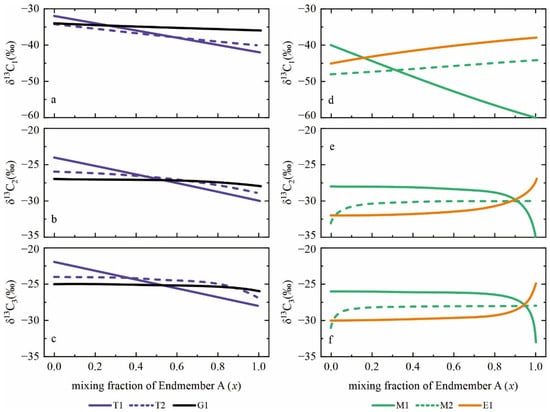
Figure 3 shows δ¹³C₁, δ¹³C₂, and δ¹³C₃ as functions of the true mixing fraction x. In the symmetric reference T1 (ρ₁ = ρ₂ = ρ₃ = 1; k₁ = k₂ = k₃ = 0.5), ω_i(x) = x for every component and all trajectories coincide with linear interpolation. Moderate asymmetry in T2 produces weak curvature, whereas the dry–wet contrast in E1 produces stronger departures. For a specified isotope contrast, curvature increases with the magnitude of log(ρ_i), or equivalently as k_i departs from 0.5. In these selected cases, methane is less curved because ρ_i lies closer to 1; high absolute methane abundance does not, by itself, suppress curvature.

Figure 3. Component-specific carbon-isotope mixing trajectories for methane, ethane, and propane in the benchmark configurations selected in Table 1. All trajectories are plotted against the bulk-gas mixing fraction of endmember A(x). (a–c) Trajectories for T1, T2, and G1: (a) δ¹³C₁, (b) δ¹³C₂, and (c) δ¹³C₃. These cases illustrate how differences in endmember isotope contrast and component-abundance asymmetry control the degree of curvature. (d–f) Trajectories for M1, M2, and E1: (d) δ¹³C₁, (e) δ¹³C₂, and (f) δ¹³C₃. M1 and M2 illustrate contrasting patterns of divergence among the component-specific effective mixing coordinates, whereas E1 provides the corresponding comparison case. In all panels, departures from bulk-fraction linear interpolation arise from component-specific abundance weighting.

Case G1 separates trajectory shape from absolute detectability. Its abundance asymmetry bends ω_i(x), but the small isotope separation limits the deviation in ‰. Whether such curvature is resolvable depends on analytical precision and sampling density; isotope contrast and abundance asymmetry must therefore be evaluated jointly. In M1 and M2, component abundance ratios diverge in opposite directions. The same x maps to different ω_i values for C₁, C₂, and C₃, so the isotope trajectories become nonlinear. This effect occurs under fixed endmembers and closed mixing, although its magnitude is specific to the selected abundance ratios and isotope contrasts. S1 and S2 serve as diagnostic controls. In S1, nearly overlapping isotopic endmembers produce negligible absolute deviations despite strong abundance asymmetry. In S2, ρ_i = 1 for all components, so the abundance-weighted model reduces exactly to linear interpolation. These cases define low-sensitivity and linear-reference limits of the framework.

4.3. Bias of Linear Approximation Under Compositional Asymmetry

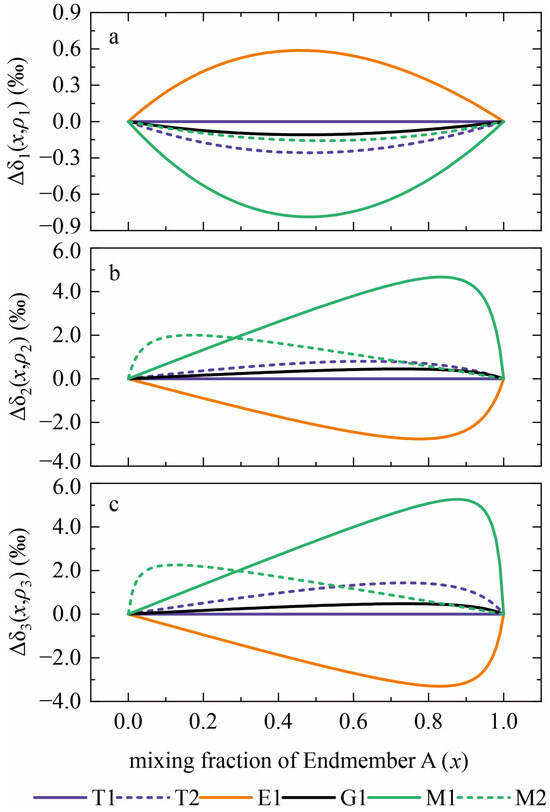
The geometric consequences are quantified with the linear-interpolation bias Δδ_i (x, ρ_i) defined in Section 2.3. Figure 4 shows the bias for methane, ethane, and propane. T1 yields Δδ_i = 0 throughout the mixing interval. T2 produces small systematic deviations, particularly for ethane and propane, whereas G1 remains modest because its isotope contrast is small. The comparison confirms that observable bias is jointly controlled by abundance asymmetry and isotope contrast.

Figure 4. Component-specific linear-interpolation bias for selected benchmark configurations from Table 1. The bias is defined as ∆δ_i(x,ρ_i) = δ¹³C_i,abundance(x) − δ¹³C_i,linear(x) for (a) methane, (b) ethane and (c) propane. T1 is exactly linear because ρ_i = 1 for all three components. T2 and G1 produce small but systematic deviations, whereas E1, M1, and M2 show larger component-specific biases. Among the configurations plotted, the largest absolute biases are approximately 0.79‰ for methane, 4.67‰ for ethane, and 5.27‰ for propane, all occurring in M1. The apparent increase in bias from methane to the higher alkanes is configuration-specific and reflects the assigned abundance ratios and isotope contrasts; it is not an intrinsic carbon-number dependence of the mixing equation.

The strongest deviations occur in E1, M1, and M2. Crucially, Equation (14) shows that absolute abundance does not enter independently: the trajectory is controlled by the abundance ratio ρ_i and the endmember isotope contrast. The trend across methane, ethane, and propane in Figure 4 arises because the benchmark library assigns progressively more asymmetric abundance ratios to the higher alkanes. In the decoupled cases, both the sign and functional form of Δδ_i differ among components because ρ₁, ρ₂, ρ₃ are unequal. A linear model can therefore yield internally inconsistent apparent mixing states even when the true system is closed and satisfies exact mass balance.

Linear interpolation can thus be substantially biased when ρ_i differs from 1. Inverse estimates based on linear mixing may be poorly conditioned or systematically shifted, particularly for components with extreme abundance ratios or limited isotope contrast. The abundance-weighted formulation removes this specific structural bias but does not, by itself, resolve uncertainty in endmember selection. Figure 3 and Figure 4 establish the mass-balance baseline for component-specific mixing and quantify when linear interpolation fails. Section 6 considers how these differences appear in wetness-indexed plots and in isotope-contrast metrics.

5. Application to a Published Field Dataset

To evaluate the framework beyond the synthetic benchmark configurations, we applied it to published molecular-composition and compound-specific carbon-isotope data from the second member of the Upper Triassic Xujiahe Formation (Xu 2 Member) in the Hexingchang Gas Field, western Sichuan Depression [27]. The purpose of this application is not to assume that binary mixing is the unique origin of the observed isotope patterns. Instead, the field data are used to test whether a geologically motivated pair of fixed endmembers can reproduce the measured C₁–C₃ isotope compositions and molecular abundances with a common bulk-gas mixing fraction. In this sense, the binary model is used as a null model: agreement supports the sufficiency of fixed-endmember mixing, whereas systematic inconsistency identifies where endmember variability, multistage charging, or other processes must be considered.

5.1. Field Dataset and Endmember Constraints

Zhao et al. [27] reported molecular and stable-isotope data for Xu 2 natural gases from the Hexingchang Gas Field. The gases are generally dry, with CH₄ contents of 91.99–99.05%, C₂H₆ contents of 0.50–3.62%, and C₃H₈ contents generally below 0.3%. Carbon-isotope compositions show a comparatively narrow range for methane, δ¹³C₁ = −33.3 to −30.7‰, but a substantially wider range for ethane, δ¹³C₂ = −27.1 to −21.9‰; propane values are mainly −27.0 to −22.3‰. Most samples exhibit an inter-component isotope reversal between ethane and propane, δ¹³C₂ > δ¹³C₃, whereas methane remains isotopically lighter than ethane. The reported analytical precision for carbon-isotope measurements is ±0.3‰.

On the basis of regional source-rock relationships and the contrasting behavior of methane and ethane isotopes, Zhao et al. [27] interpreted the Hexingchang gases as being dominated by high- to overmature coal-derived gas with a subordinate contribution from isotopically lighter marine oil-type cracked gas. In their representative comparison, the Xu 2 coal-derived gas from the Qiongxi area has a methane isotope composition close to that of the proposed oil-type endmember, whereas the two sources differ by approximately 13‰ in δ¹³C₂. This contrast was used to explain the relatively small variation in δ¹³C₁ but much larger variation in δ¹³C₂, and the oil-type contribution was estimated to reach approximately 35% locally.

We therefore use Xu 2 gases from the Qiongxi area as the coal-derived endmember population. Published Qiongxi samples provide both molecular compositions and C₁–C₃ carbon-isotope compositions; for example, Qiongxi 10 contains 93.57% CH₄, 3.85% C₂H₆, and 0.59% C₃H₈, with δ¹³C₁ = −33.2‰, δ¹³C₂ = −22.8‰, and δ¹³C₃ = −22.8‰ [28]. The reported precision of the carbon-isotope measurements is scenario-based, i.e., ±0.3‰ and ±0.5‰.

The geological identity of the isotopically light marine contributor to Hexingchang is less tightly constrained. Zhao et al. [27] documented an overmature oil-type gas in the Xu 2 Member of Well Tongshen 1, with δ¹³C₁ = −31.6‰, δ¹³C₂ = −35.6‰, and δ¹³C₃ = −32.9‰, but complete C₁–C₃ molecular-abundance data required by the present formulation are not available for this endmember in the compiled dataset. We therefore use gases from the Fuling (Jiaoshiba) shale-gas field only as compositional and isotopic analogues of an overmature marine oil-type endmember, rather than implying that Jiaoshiba gas was the actual geological source of the Hexingchang accumulation.

This choice is supported by the independent geochemical characterization of the Jiaoshiba gases. They were generated from overmature, type-I organic matter in the Wufeng–Longmaxi marine shale and were classified as oil-derived gases by Dai et al. [29]. They are extremely dry, with average CH₄, C₂H₆, and C₃H₈ contents of approximately 98.44%, 0.66%, and 0.02%, respectively. Complete C₁–C₃ isotope and abundance data are available for multiple individual samples, with a reported carbon-isotope precision of ±0.5‰.

Endmember selection was not based on minimizing the isotope residuals of the Hexingchang samples. Instead, candidate endmembers were first required to satisfy independent geological and geochemical criteria: the coal-derived endmember had to represent high- to overmature Xu 2 coal-derived gas, whereas the marine analogue had to represent an independently characterized overmature oil-derived gas and provide complete C₁–C₃ molecular and isotope data. Samples with complete measurements were then treated collectively as endmember populations in the sensitivity analysis described below.

5.2. Coupled C₁–C₃ Test of the Fixed-Endmember Model

For the field application, endmember A denotes the high- to overmature coal-derived gas represented by the Qiongxi population, whereas endmember B denotes the overmature marine oil-type analogue represented by the Jiaoshiba population. For each candidate endmember pair, the component-specific abundance ratio (ρ_i) and its normalized form (k_i) were calculated from Equations (10) and (12), respectively. These quantities describe the abundance asymmetry experienced by each hydrocarbon component independently of the bulk-gas mixing fraction.

The Qiongxi 10–JY42-2 pair is used as a representative example because both samples have complete C₁–C₃ molecular and carbon-isotope data. Qiongxi 10 contains 93.57% CH₄, 3.85% C₂H₆, and 0.59% C₃H₈, whereas JY42-2 contains 98.89% CH₄, 0.69% C₂H₆, and 0.02% C₃H₈. These abundances give ρ₁ = 1.057, ρ₂ = 0.179, ρ₃ = 0.034, and therefore k₁ = 0.486, k₂ = 0.848, k₃ = 0.967 (Table S1). The methane abundance is thus close to the symmetric condition k_i = 0.5, whereas ethane and especially propane are strongly asymmetric. Consequently, a common bulk-gas mixing fraction is expected to map onto substantially different effective coordinates for C₁, C₂, and C₃. This field-derived configuration therefore provides a natural example of the component-specific nonlinearity illustrated by the synthetic experiments in Section 4.

For an observed Hexingchang sample, the effective coordinate defined in Equation (8) is not measured directly, but can be inferred from the isotope composition. Rearranging Equation (9) gives the effective mixing coordinate implied by component i:

$${\omega }_{i,\mathit{obs}}={\displaystyle \frac{{\mathit{\delta }}^{13}{C}_{i,\mathit{obs}}-{\mathit{\delta }}^{13}{C}_{\mathit{iB}}}{{\mathit{\delta }}^{13}{C}_{\mathit{iA}}-{\mathit{\delta }}^{13}{C}_{\mathit{iB}}}}$$

Here, ω_i,obs has the same physical meaning as ω_i(x) in Section 2.2: it is the fraction of component i in the mixture that is supplied by endmember A, as implied by the measured isotope composition. The subscript “obs” distinguishes the value inferred from a field observation from the forward-model value calculated for a prescribed x.

For a physically admissible fixed-endmember mixture, 0 ≤ ω_i,obs ≤ 1, after analytical and endmember uncertainties are taken into account. A value outside this interval indicates that the observed isotope composition is not bracketed by the selected endmembers and therefore cannot be reproduced by that particular binary endmember pair. If δ¹³C_i,A = δ¹³C_i,B, the isotope composition of component i contains no information on mixing fraction and ω_i,obs cannot be independently resolved from that component.

For components with distinct endmember isotope compositions, substitution of ω_i,obs into the inverse of Equation (11) gives the component-specific isotope-derived estimate of the bulk-gas mixing fraction:

$${\widehat{x}}_{i,\mathit{iso}}={\displaystyle \frac{{\omega }_{i,\mathit{obs}}{\rho }_i}{1-{\omega }_{i,\mathit{obs}}+{\omega }_{i,\mathit{obs}}{\rho }_i}}$$

The distinction between the observed effective coordinate ω_i,obs and the component-specific isotope-derived mixing-fraction estimate ${\widehat{x}}_{i,\mathit{iso}}$ is important. The effective coordinates ω_1,obs, ω_2,obs, and ω_3,obs are generally not expected to be equal because each component has a different abundance ratio. In contrast, all components in a fixed-endmember binary mixture must correspond to the same physical bulk-gas mixing fraction. The principal isotope-consistency condition is therefore ${\widehat{x}}_{1,\mathit{iso}}\approx {\widehat{x}}_{2,\mathit{iso}}\approx {\widehat{x}}_{3,\mathit{iso}}$, within the uncertainties associated with the isotope measurements and endmember parameters. Large systematic differences among ${\widehat{x}}_{1,\mathit{iso}}$, ${\widehat{x}}_{2,\mathit{iso}}$, and ${\widehat{x}}_{3,\mathit{iso}}$ indicate that the selected fixed-endmember pair is insufficient to reproduce the observed C₁–C₃ isotope composition.

Because individual components differ in their isotope contrast and abundance asymmetry, their resolving power is also unequal. A component with a small endmember isotope contrast can yield a poorly constrained ${\widehat{x}}_{i,\mathit{iso}}$, even when its trajectory is mathematically monotonic. Conversely, a component with a large isotope contrast may constrain the mixing fraction more strongly. The component-specific estimates are therefore used as diagnostic quantities rather than simply averaged. A common estimate of the bulk-gas mixing fraction, ${\widehat{x}}_{\mathit{iso}}$, is subsequently obtained from the uncertainty-weighted joint objective function described in Section 3.

The joint isotope fit alone is not sufficient to establish consistency with the binary model. The same fitted mixing fraction must also satisfy molecular mass balance. For each component, the predicted abundance is

$$n_{i,\mathit{pred}}=n_i\left({\widehat{x}}_{\mathit{iso}}\right)={\widehat{x}}_{\mathit{iso}}{n}_{i,A}+(1-{\widehat{x}}_{\mathit{iso}})n_{i,B}$$

Predicted C₁–C₃ abundances were therefore compared with the measured molecular compositions of the Hexingchang samples. Wetness was calculated from the same predicted composition using the definition adopted in Section 3. This provides an independent compositional test because isotope values may occasionally be reproduced by a selected endmember pair even when the corresponding molecular abundances are inconsistent with the same bulk-gas mixing fraction.

For comparison, the molecular composition also provides an independent estimate of the bulk-gas mixing fraction. For each component,

$${\widehat{x}}_{i,\mathit{mol}}={\displaystyle \frac{n_{i,\mathit{obs}}-n_{i,B}}{n_{i,A}-n_{i,B}}}$$

A joint molecular-composition-derived estimate, ${\widehat{x}}_{\mathit{mol}}$, was obtained by minimizing the C₁–C₃ molecular-composition residual sum of squares,

$${\widehat{x}}_{\mathit{mol}}=\underset{0\le x\le 1}{\mathrm{a}\mathit{rg}\min }{\displaystyle \sum _{i=1}^3}{\left[n_{i,\mathit{obs}}-n_i\left(x\right)\right]}^2$$

The difference between ${\widehat{x}}_{\mathit{iso}}$ and ${\widehat{x}}_{\mathit{mol}}$ therefore provides an independent measure of consistency between the isotope and molecular-composition constraints.

We therefore evaluate each field sample using three nested criteria. First, the observed C₁–C₃ isotope values must be bracketed by the selected endmembers within uncertainty. Second, the component-specific isotope estimates ${\widehat{x}}_{i,\mathit{iso}}$ must be mutually consistent with the joint isotope-derived mixing fraction ${\widehat{x}}_{\mathit{iso}}$. Third, the joint isotope-derived mixing fraction ${\widehat{x}}_{\mathit{iso}}$ must predict molecular abundances and wetness compatible with the observed gas composition. Satisfaction of all three conditions indicates that the fixed-endmember binary model is sufficient to describe the sample within the stated uncertainties. Failure of one or more criteria rejects that particular endmember pair as a complete description of the sample, but does not by itself exclude mixing involving variable endmembers, additional sources, or multistage charging.

The representative Qiongxi 10–JY42-2 pair illustrates why the coupled test is necessary. Its nearly symmetric methane abundance produces k₁ ≈ 0.5, whereas the much lower C₂ and C₃ abundances of the marine analogue give k₂ = 0.848 and k₃ = 0.967. Consequently, the three isotope components respond very differently to the same physical x. A conventional isotope-only comparison can therefore obscure whether apparently compatible C₁–C₃ values actually correspond to a common bulk-gas mixture. The component-specific inversion developed here makes this consistency directly testable. The quantitative assessment was then repeated across the set of geologically admissible Qiongxi–Jiaoshiba endmember combinations rather than relying on the representative pair alone.

5.3. Sensitivity to Endmember Selection and Model Consistency

Natural-gas endmembers are populations rather than exact compositions, so the field-data evaluation was repeated across the full set of independently constrained candidate endmembers rather than being based on a single optimized pair. Seven Qiongxi Xu 2 samples with complete C₁–C₃ molecular and carbon-isotope data were retained as coal-derived endmember candidates [28], and six Jiaoshiba samples with complete C₁–C₃ data from the internally consistent dataset of Dai et al. [7] were retained as overmature marine oil-type analogues (Table S1). Nine Hexingchang samples measured by Zhao et al. [27] contained complete C₁–C₃ molecular and carbon-isotope data and were retained as field observations (Table S1). This yielded 42 candidate endmember pairs and 378 endmember-pair–sample evaluations (Tables S2 and S3).

The field-derived endmember ensemble shows a strongly component-dependent abundance asymmetry. Across the 42 endmember pairs, k₁ ranges only from 0.485 to 0.495, whereas k₂ ranges from 0.689 to 0.873 and k₃ from 0.857 to 0.973 (Table S2). Thus, methane is consistently close to the abundance-symmetric condition, whereas ethane and propane are strongly asymmetric. Using Equation (18), the corresponding maximum absolute bias of linear interpolation is only 0–0.056‰ for methane, but 2.26–6.04‰ for ethane and 5.92–12.04‰ for propane (Table S2). The field endmembers therefore reproduce the component-specific nonlinearity identified independently in the synthetic benchmarks.

Analytical uncertainty was propagated separately from endmember-population variability. The reported carbon-isotope precision is ±0.3‰ for the Hexingchang dataset and ±0.5‰ for the Jiaoshiba dataset. The Qiongxi values used here are compiled by Ni et al. [28] from an earlier published dataset, and a sample-specific analytical precision is not reported with those entries. We therefore treated the Qiongxi isotope uncertainty as a sensitivity parameter, using ±0.5‰ as a conservative baseline and ±0.3‰ as an alternative scenario. For a specified endmember pair, the effective isotope uncertainty was calculated by Equation (21). Molecular-abundance uncertainty could not be propagated in the same manner because comparable analytical errors were not reported for all three published datasets; molecular composition was therefore used as an independent deterministic consistency test.

For each field sample, nominal endmember bracketing was first recorded for C₁–C₃, after which the uncertainty-weighted joint isotope objective defined in Section 3 was minimized over 0 ≤ x ≤ 1. For screening purposes, $\mathsf{\Phi }\left({\widehat{x}}_{\mathit{iso}}\right)$≤ 5.991, corresponding to the 95% chi-square value for two nominal degrees of freedom, was used as a reference criterion. Because the Qiongxi uncertainty is scenario-based, this threshold is used only as a diagnostic screen and not as a formal hypothesis test.

Under the conservative ±0.5‰ Qiongxi uncertainty scenario, only two Hexingchang samples produced nominally bracketed interior solutions that satisfied the joint C₁–C₃ isotope screening criterion. A127-4645 was consistent with 11 of the 42 candidate endmember pairs, whereas B204H was consistent with six (Table S4). No other sample satisfied both conditions. B101 and B209 gave relatively low joint isotope misfits only at the ${\widehat{x}}_{\mathit{iso}}$ = 1 boundary and were not nominally bracketed by any candidate pair across all three isotope components; these solutions therefore represent Qiongxi-like endpoint behavior rather than evidence for an interior binary mixture. Reducing the assumed Qiongxi isotope uncertainty to ±0.3‰ reduced the number of acceptable pairs to three for A127-4645 and one for B204H, without changing the identity of the samples that support interior solutions (Table S4).

The best isotope fit for A127-4645 was obtained with Qiongxi 13 and JY12-4, giving ${\widehat{x}}_{\mathit{iso}}$= 0.415 and an isotope RMSE of 0.56‰. The component-specific estimates were ${\widehat{x}}_{1,\mathit{iso}}$ = 0.447, ${\widehat{x}}_{2,\mathit{iso}}$ = 0.448, and ${\widehat{x}}_{3,\mathit{iso}}$ = 0.214. In contrast, the molecular abundances of the same sample gave component-specific mixing estimates of 0.055, 0.111, and 0.246 and a joint composition estimate of ${\widehat{x}}_{\mathit{mol}}$ = 0.072. At the isotope-derived ${\widehat{x}}_{\mathit{iso}}$, the predicted wetness was 2.30%, compared with an observed value of 1.19% (Table S3). B204H showed a similar discrepancy. Its best isotope fit, using Qiongxi 14 and JY42-2, gave ${\widehat{x}}_{\mathit{iso}}$ of 0.892 and an isotope RMSE of 0.58‰, whereas the joint molecular-composition estimate was ${\widehat{x}}_{\mathit{mol}}$ = 0.579. The isotope-derived model predicted a wetness of 1.61%, compared with an observed value of 1.05% (Table S3). The large spread among the component-specific isotope estimates in this case also illustrates the unequal resolving power of individual hydrocarbons when their endmember isotope contrasts differ.

Thus, isotope agreement alone does not establish a complete fixed-endmember mixing solution. Some Hexingchang samples can be reproduced reasonably well in C₁–C₃ isotope space by independently constrained Qiongxi–Jiaoshiba endmember pairs, but the same mixing fractions do not reproduce their molecular compositions. These results do not reject the broader geological interpretation that the Hexingchang gases contain both coal-derived and marine oil-type contributions. Instead, they show that the field population cannot be represented by a single pair of fixed-endmember compositions. Endmember heterogeneity, multistage charging, additional source contributions, or other departures from the fixed binary null model are required to reconcile the isotope and molecular-composition constraints.

6. Discussion

6.1. Component-Specific Mixing Geometry and Isotope Contrasts

Mature to overmature natural-gas systems commonly show comparatively systematic methane isotope trends together with greater curvature or variability in ethane and propane. Such behavior is particularly conspicuous in dry gases, where the low abundances of C₂ and C₃ increase the potential influence of endmember heterogeneity, analytical uncertainty, and abundance contrasts [4,6,9,10]. Individual-component isotope rollover should, however, be distinguished from simple curvature, analytical scatter, and extrema in isotope-contrast metrics [9,10].

In the abundance-weighted binary model, the isotope composition of each hydrocarbon is controlled by its component-specific effective mixing coordinate, ω_i(x). When ρ₁, ρ₂, and ρ₃ differ, the same physical bulk-gas mixing fraction x corresponds to different effective mixing positions for methane, ethane, and propane. This divergence among effective mixing coordinates produces component-specific curvature and different apparent mixing responses even though all components belong to the same physical mixture.

The stronger curvature of C₂ and C₃ in the selected benchmark cases is therefore not an intrinsic carbon-number effect. It arises because their assigned endmember abundance ratios are more asymmetric than that of methane. The field-derived endmember combinations examined in Section 5 show the same tendency: ρ₁ remains relatively close to unity, whereas ρ₂ and particularly ρ₃ depart much more strongly from unity. This explains why higher hydrocarbons can respond much more strongly to abundance-weighted mixing than methane.

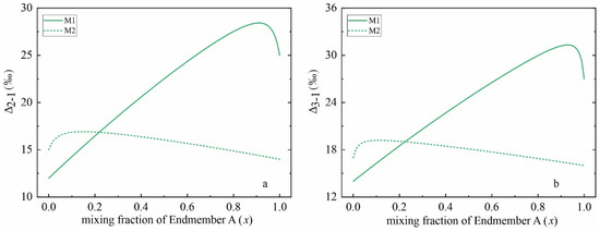
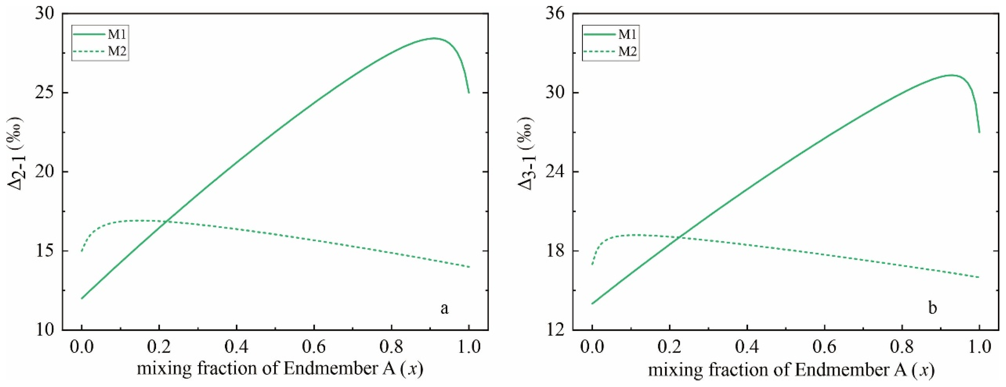
Differences among the effective mixing coordinates also explain why isotope-contrast metrics can become non-monotonic even when each individual isotope trajectory remains monotonic. A difference between two monotonic functions need not itself be monotonic. Consequently, quantities such as Δ₂₋₁ = δ¹³C₂ − δ¹³C₁, Δ₃₋₁ = δ¹³C₃ − δ¹³C₁ and Δ₃₋₂ = δ¹³C₃ − δ¹³C₂ may develop local extrema solely because the component-specific effective coordinates differ. These features are therefore more appropriately described as isotope-contrast extrema rather than isotope rollover. Figure 5 illustrates this geometric effect for the decoupled benchmark configurations.

Figure 5. Non-monotonic isotope-contrast metrics versus bulk-gas mixing fraction for two oppositely decoupled abundance scenarios (M1, solid; M2, dashed). Panel (a) shows Δ_2–1 = δ¹³C₂ − δ¹³C₁ and panel (b) shows Δ_3–1 = δ¹³C₃ − δ¹³C₁. The extrema arise from component-specific effective mixing coordinates and do not imply non-monotonicity of any individual δ¹³C_i value. Replotting against a monotonic wetness coordinate would preserve the y-values and extrema while shifting their positions along the horizontal axis.

6.2. Wetness as a Reparameterization of Mixing

Gas wetness, W = 100 × (C₂ + C₃)/(C₁ + C₂ + C₃), is commonly used as a compositional coordinate for isotope trends. For fixed binary endmembers, let H_A = n_1,A + n_2,A + n_3,A and H_B = n_1,B + n_2,B + n_3,B. The wetness of the mixture is

$$W\left(x\right)=100{\displaystyle \frac{x\left(n_{2,A}+n_{3,A}\right)+(1-x)(n_{2,B}+n_{3,B})}{x{H}_A+(1-x)H_B}}$$

(23)

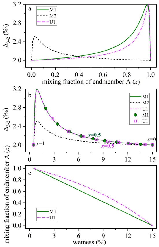
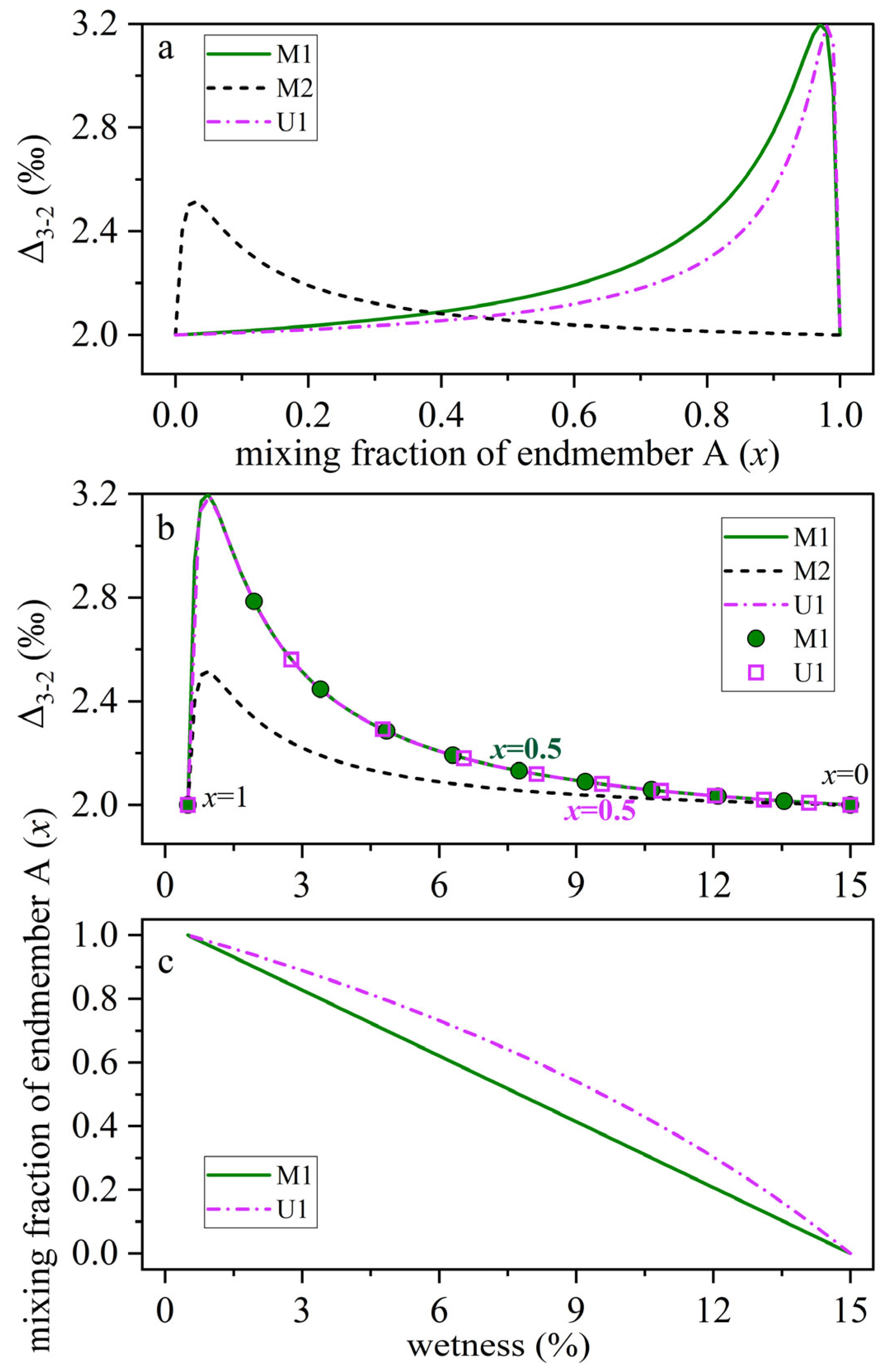
When the two endmembers have different wetness values, W(x) is a monotonic linear-fractional function of the physical mixing fraction. It is linear when H_A = H_B and generally nonlinear when H_A ≠ H_B. The normalized benchmark configurations therefore provide a linear wetness–x mapping, whereas configuration U1 demonstrates the nonlinear case associated with unequal-total C₁–C₃ abundances.

Configuration U1 provides an explicit unequal-total example. It retains the within-hydrocarbon composition and isotope compositions of M1 but has H_A = 0.60 and H_B = 1.00. Its endmember wetness values therefore remain W_A = 0.5% and W_B = 15%, whereas the mapping between x and wetness becomes

$$W_{U1}\left(x\right)={\displaystyle \frac{15-14.7x}{1-0.4x}}$$

(24)

For example, at x = 0.5, U1 gives W = 9.56%, whereas the corresponding linear mapping between the same endmember wetness values gives W = 7.75%. Equal increments in the physical mixing fraction therefore no longer correspond to equal increments along the wetness axis when the total hydrocarbon abundances of the two endmembers differ.

This distinction is important because wetness is a reparameterization of the mixing path rather than an independent isotope-generating variable. Replotting an isotope trajectory against wetness can relocate existing features along the horizontal axis and, when H_A ≠ H_B, nonlinearly compress or stretch portions of the trajectory. It can therefore change apparent slopes and the spacing of observations sampled at equal increments of x. However, provided that W(x) is one-to-one, the transformation cannot create a new extremum or alter the vertical range of an isotope value or isotope-contrast metric.

Figure 6 illustrates this behavior. M1 and U1 follow different trajectories when parameterized by the physical mixing fraction x, but they trace the same Δ₃₋₂–wetness locus because U1 differs from M1 only by proportional scaling of the C₁–C₃ abundances of endmember A. The nonlinear x–wetness relation for U1 changes how this locus is traversed, as shown by the non-uniform spacing of points representing equal increments of x, but it does not generate new isotope extrema. Wetness-indexed curvature or slope changes should therefore be interpreted as possible expressions of mixing-path reparameterization rather than, by themselves, as evidence for an additional isotope process.

Figure 6. Wetness reparameterization of the propane–ethane carbon-isotope contrast under equal and unequal hydrocarbon totals. (a) Δ₃₋₂ = δ¹³C₃ − δ¹³C₂ plotted against the bulk-gas mixing fraction of endmember A (x) for M1, M2, and U1. Configuration U1 retains the within-hydrocarbon composition and isotope compositions of M1 but has unequal-total C₁–C₃ abundances (H_A = 0.60, H_B = 1.00). (b) The same isotope contrast plotted against gas wetness. Symbols for M1 and U1 mark equal increments of x, illustrating the non-uniform mapping between x and wetness for U1. (c) Relation between x and wetness for M1 and U1. The mapping is linear for M1 and nonlinear for U1. Wetness therefore relocates and stretches or compresses pre-existing isotope features but does not create new extrema.

6.3. Field-Data Implications of the Fixed-Endmember Binary Test

The Hexingchang application demonstrates that isotope consistency alone does not establish a fully self-consistent fixed-endmember binary mixture. Only a limited subset of the tested endmember–observation combinations satisfies the isotope-consistency criteria defined in Section 5, and the sensitivity analysis does not alter this qualitative result.

Combinations that reproduce the C₁–C₃ isotope compositions do not necessarily reproduce the molecular composition with the same bulk-gas mixing fraction. This discrepancy is particularly clear for A127-4645, for which the isotope-derived estimate (${\widehat{x}}_{\mathit{iso}}$ = 0.415) differs substantially from the independently derived molecular-composition estimate (${\widehat{x}}_{\mathit{mol}}$ = 0.072). Similar inconsistency is observed for B204H. Thus, a low isotope misfit indicates only that the isotope observations can be approximated by a common mixing fraction for the specified endpoints; it does not demonstrate consistency of the complete molecular–isotopic system.

The field results therefore do not exclude a broader mixed origin for the Hexingchang gases. Rather, they indicate that a single invariant pair of Qiongxi-like and Jiaoshiba-like endmembers is generally insufficient to reproduce both isotope compositions and molecular abundances with one common bulk-gas mixing fraction. The fixed-endmember binary model is consequently most useful as a diagnostic null model for identifying where additional geological or geochemical complexity is required.

6.4. Geological Implications and Model Limits

Natural-gas accumulations commonly integrate multiple source intervals, maturity stages, charging episodes, and preservation histories. Endmembers in the present framework should therefore be interpreted as effective gas packages rather than necessarily as discrete and coeval generation products [5,10,25,30]. In the Hexingchang application, the Qiongxi and Jiaoshiba gases are accordingly used as independently constrained compositional and isotopic analogues rather than as uniquely defined literal source gases for every field sample.

Failure of a particular fixed-endmember pair does not imply the absence of mixing. Instead, it indicates that one or more assumptions of the simple model may be inadequate. Natural endmembers may vary spatially or temporally, and different charging episodes may involve different source contributions. Secondary cracking, selective retention or leakage, diffusion, desorption, and other post-generation processes may further modify molecular abundances, isotope compositions, or both [11,14,15,31,32,33,34]. Such processes may remain compatible with overall mass balance while violating the assumption of mixing between two invariant endmembers.

The formulation extends directly to ternary mixing by summing the component-specific isotope inventories over three endmembers. In the practical delta approximation, the isotope composition of component i becomes a component-abundance-weighted average of the three endmember values:

$${\mathit{\delta }}^{13}{C}_i\approx {\displaystyle \frac{{\mathbf{\sum }}_{j=1}^3{x}_j{n}_{\mathit{ij}}{\mathit{\delta }}^{13}{C}_{\mathit{ij}}}{{\mathbf{\sum }}_{j=1}^3{x}_j{n}_{\mathit{ij}}}}, x_j\ge 0,{\displaystyle \mathbf{\sum }_{j=1}^3}{x}_j=1$$

(25)

Unlike binary mixing, however, ternary mixing has two independent mixing fractions. Consequently, the one-dimensional monotonicity result derived above does not generally extend to arbitrary paths through the ternary mixing domain or to their projection onto wetness. Nevertheless, because the weights are positive, the isotope composition of each component remains bounded by the corresponding endmember values. Distinguishing ternary mixing from evolving endmembers or fractionating processes therefore requires additional independent compositional, isotopic, or geological constraints.

The model also has important identifiability limits. Three isotope observations alone cannot uniquely determine unknown endmember isotope compositions, component abundance ratios, and mixing fractions simultaneously. Independent molecular-composition data, geological constraints, multiple samples, and realistic uncertainty estimates are therefore essential. Analytical uncertainty is particularly important for the low-abundance C₂ and C₃ components of very dry gases, while endmember heterogeneity introduces an additional source of uncertainty that should be distinguished from measurement error. The present formulation can be extended to three or more endmembers, but additional independent mixing fractions remove the simple one-dimensional constraint of the binary model.

Routine analytical uncertainty also limits the practical resolution of component-specific mixing trajectories. From the derivative of the abundance-weighted mixing relation, first-order propagation of an isotope uncertainty σ_δ,i gives

$${\sigma }_{x,i}\approx {\displaystyle \frac{{\sigma }_{\mathit{\delta },i}}{\left|d{\mathit{\delta }}^{13}{C}_i/\mathit{dx}\right|}}={\sigma }_{\mathit{\delta },i}{\displaystyle \frac{{\left[x+\left(1-x\right){\rho }_i\right]}^2}{{\left|{\mathit{\delta }}^{13}{C}_{i,A}-{\mathit{\delta }}^{13}{C}_{i,B}\right|\rho }_i}}$$

Thus, the inferred mixing fraction is best resolved where the endmember isotope contrast is large, and the local trajectory is steep. It decreases where isotope contrasts are small, or the trajectory is flat or less steep. In very dry gases, the low abundances of C₂ and C₃ may further increase uncertainty in their isotope and molecular-composition measurements. Small apparent differences among component-specific trajectories should therefore be interpreted only when they exceed the relevant analytical uncertainty.

Finally, the monotonicity result provides an important diagnostic boundary. For positive ρi and distinct fixed isotope endpoints, each individual δ¹³C_i(x) trajectory is strictly monotonic with the physical binary-mixing fraction. Fixed-endmember binary mixing can therefore produce curvature, divergence among component-specific mixing responses, and non-monotonic isotope-contrast metrics, but it cannot produce a true rollover of an individual hydrocarbon-isotope trajectory. An observed individual-component rollover therefore requires at least one assumption of the fixed binary model to be relaxed, for example through evolving or multiple endmembers, reaction, transport-related isotope fractionation, or another open-system process. This distinction defines the principal diagnostic boundary of the abundance-weighted framework.

7. Conclusions

Four conclusions follow from the analysis. (1) Carbon-isotope mixing is component-weighted. The effective coordinate ω_i(x) = x/[x + (1 − x) ρ_i] maps the bulk-gas mixing fraction to the fraction of component i supplied by an endmember. Linear interpolation is exact only when ρ_i = 1. (2) The bias of linear interpolation is governed jointly by the endmember isotope contrast and the component abundance ratio. The larger biases of ethane and propane in the benchmark cases arise from their assigned abundance contrasts, not from an intrinsic carbon-number effect. (3) Different effective coordinates result in deviations of C₁−C₃ trajectories and can produce local extrema in isotope-contrast metrics even when each individual δ¹³C_i value remains monotonic. For fixed binary endmembers with different wetness values, wetness is a monotonic reparameterization of the mixing path that can shift and stretch or compress existing features along the horizontal axis, but cannot create new extrema or change their amplitudes. (4) A true rollover of an individual hydrocarbon-isotope trajectory lies outside the fixed-endmember binary model and requires evolving or multiple endmembers, reaction, transport fractionation, or another open-system process. The abundance-weighted framework should therefore be used as a mass-balance baseline before more complex mechanisms are invoked.

References

- Schoell, M. Genetic characterization of natural gases. Am. Assoc. Petrol. Geol. Bull. 1983, 67, 2225–2238. [Google Scholar] [CrossRef] [Scilit]
- Whiticar, M.J. Carbon and hydrogen isotope systematics of bacterial formation and oxidation of methane. Chem. Geol. 1999, 161, 291–314. [Google Scholar] [CrossRef] [Scilit]
- Dai, J. Identification and distinction of various alkane gases. Sci. China Ser. B Chem. Life Sci. Earth Sci. 1992, 35, 1246–1257. [Google Scholar]
- Cesar, J.; Nightingale, M.; Becker, V.; Mayer, B. Stable carbon isotope systematics of methane, ethane and propane from low-permeability hydrocarbon reservoirs. Chem. Geol. 2020, 558, 119907. [Google Scholar] [CrossRef] [Scilit]
- Tilley, B.; Muehlenbachs, K. Isotope reversals and universal stages and trends of gas maturation in sealed, self-contained petroleum systems. Chem. Geol. 2013, 339, 194–204. [Google Scholar] [CrossRef] [Scilit]
- Dai, J.; Zou, C.; Liao, S.; Dong, D.; Ni, Y.; Huang, J.; Wu, W.; Gong, D.; Huang, S.; Hu, G. Geochemistry of the extremely high thermal maturity Longmaxi shale gas, southern Sichuan Basin. Org. Geochem. 2014, 74, 3–12. [Google Scholar] [CrossRef] [Scilit]
- Dai, J.; Zou, C.; Dong, D.; Ni, Y.; Wu, W.; Gong, D.; Wang, Y.; Huang, S.; Huang, J.; Fang, C.; et al. Geochemical characteristics of marine and terrestrial shale gas in China. Mar. Petrol. Geol. 2016, 76, 444–463. [Google Scholar] [CrossRef] [Scilit]
- Ni, Y.; Gao, J.; Chen, J.; Liao, F.; Liu, J.; Zhang, D. Gas generation and its isotope composition during coal pyrolysis: Potential mechanism of isotope rollover. Fuel 2018, 231, 387–395. [Google Scholar] [CrossRef] [Scilit]
- Ni, Y.; Dong, D.; Yao, L.; Chen, J.; Liang, X.; Liu, F.; Li, J.; Guo, J.; Gao, J. Geochemical characteristics and origin of shale gases from Sichuan Basin, China. Front. Earth Sci. 2022, 10, 861040. [Google Scholar] [CrossRef] [Scilit]
- Zumberge, J.; Ferworn, K.; Brown, S. Isotopic reversal (‘rollover’) in shale gases produced from the Mississippian Barnett and Fayetteville formations. Mar. Petrol. Geol. 2012, 31, 43–52. [Google Scholar] [CrossRef] [Scilit]
- Hao, F.; Zou, H. Cause of shale gas geochemical anomalies and mechanisms for gas enrichment and depletion in high-maturity shales. Mar. Petrol. Geol. 2013, 44, 1–12. [Google Scholar] [CrossRef] [Scilit]
- Xia, X.; Chen, J.; Braun, R.; Tang, Y. Isotopic reversals with respect to maturity trends due to mixing of primary and secondary products in source rocks. Chem. Geol. 2013, 339, 205–212. [Google Scholar] [CrossRef] [Scilit]
- Xia, X.; Gao, Y. Depletion of 13C in residual ethane and propane during thermal decomposition in sedimentary basins. Org. Geochem. 2018, 125, 121–128. [Google Scholar] [CrossRef] [Scilit]
- Zhai, C.B.; Tao, C.; Zou, Y.; Yang, Z.H.; Ye, X.; Nie, H.K. End-member mixing model for methane carbon isotope fractionation during shale gas desorption and its application. ACS Omega 2024, 9, 36993–37001. [Google Scholar] [CrossRef] [Scilit]
- Burruss, R.C.; Laughrey, C.D. Carbon and hydrogen isotopic reversals in deep basin gas: Evidence for limits to the stability of hydrocarbons. Org. Geochem. 2010, 41, 1285–1296. [Google Scholar] [CrossRef] [Scilit]
- Laughrey, C.D. Produced Gas and Condensate Geochemistry of the Marcellus Formation in the Appalachian Basin: Insights into Petroleum Maturity, Migration, and Alteration in an Unconventional Shale Reservoir. Minerals 2022, 12, 1222. [Google Scholar] [CrossRef] [Scilit]
- Gao, L.; Schimmelmann, A.; Tang, Y.; Mastalerz, M. Isotope rollover in shale gas observed in laboratory pyrolysis experiments: Insight to the role of water in thermogenesis of mature gas. Org. Geochem. 2014, 68, 95–106. [Google Scholar] [CrossRef] [Scilit]
- Cheng, B.; Li, S.; Xu, J.; Liao, Z. Gaseous hydrocarbons cracking in shale: Mechanism, impact and resource significance. Earth-Sci. Rev. 2025, 270, 105211. [Google Scholar] [CrossRef] [Scilit]
- Langmuir, C.H.; Vocke, R.D.; Hanson, G.N.; Hart, S.R. A general mixing equation with applications to Icelandic basalts. Earth Planet. Sci. Lett. 1978, 37, 380–392. [Google Scholar] [CrossRef] [Scilit]
- Berner, U.; Faber, E. Maturity related mixing model for methane, ethane and propane, based on carbon isotopes. Org. Geochem. 1988, 13, 67–72. [Google Scholar] [CrossRef] [Scilit]
- Xia, X.Y.; Li, C.Y.; Zhao, L. Mixing effects of natural gases on genetic identification with isotopes. Pet. Explor. Dev. 1998, 25, 89–90+93. [Google Scholar]
- Chung, H.M.; Gormly, J.R.; Squires, R.M. Origin of gaseous hydrocarbons in subsurface environment: Theoretical considerations of carbon isotope distribution. Chem. Geol. 1988, 71, 97–103. [Google Scholar] [CrossRef] [Scilit]
- Prinzhofer, A.; Huc, A. Genetic and post-genetic molecular and isotopic fractinations in natural gases. Chem. Geol. 1995, 126, 281–290. [Google Scholar] [CrossRef] [Scilit]
- Liu, Q.Y.; Wu, X.Q.; Wang, X.F.; Jin, Z.J.; Zhu, D.Y.; Meng, Q.Q.; Huang, S.P.; Liu, J.Y.; Fu, Q. Carbon and hydrogen isotopes of methane, ethane, and propane: A review of genetic identification of natural gas. Earth-Sci. Rev. 2019, 190, 247–272. [Google Scholar] [CrossRef] [Scilit]
- Dai, J.X. Giant Gas Fields and Gas Sources in China; Petroleum Industry Press: Beijing, China, 2024. [Google Scholar]
- Ni, Y.; Zhang, J.; Yao, L.; Dong, G.; Wang, Y.; Wang, L.; Chen, J. Application of carbon and hydrogen isotopes in the natural gas origin study. Nat. Gas. Geosci. 2024, 35, 1897–1909. [Google Scholar]
- Zhao, S.; Liu, Y.H.; Wang, L.H.; Ni, Y.Y.; Chen, J.P.; Di, M.X.; Zheng, Q.; Zhang, J.C.; Feng, S.Y.; Bai, L.X. Origin and source analysis of natural gas in the second member of Xujiahe Formation in Hexingchang Gas Field, Sichuan Basin. Nat. Gas. Geosci. 2026, 37, 1–12. [Google Scholar]
- Ni, Y.Y.; Liao, F.R.; Yao, L.M.; Gao, J.L.; Zhang, D.J. Hydrogen isotope of natural gas from the Xujiahe Formation and its implications for water salinization in central Sichuan Basin, China. J. Nat. Gas. Geosci. 2019, 4, 215–230. [Google Scholar] [CrossRef] [Scilit]
- Dai, J.; Ni, Y.; Gong, D.; Feng, Z.; Liu, D.; Peng, W.; Han, W. Geochemical characteristics of gases from the largest tight sand gas field (Sulige) and shale gas field (Fuling) in China. Mar. Petrol. Geol. 2017, 79, 426–438. [Google Scholar] [CrossRef] [Scilit]
- Dai, J.; Li, J.; Luo, X.; Zhang, W.; Hu, G.; Ma, C.; Guo, J.; Ge, S. Stable carbon isotope compositions and source rock geochemistry of the giant gas accumulations in the Ordos Basin, China. Org. Geochem. 2005, 36, 1617–1635. [Google Scholar] [CrossRef] [Scilit]
- Zhang, T.; Krooss, B.M. Experimental investigation on the carbon isotope fractionation of methane during gas migration by diffusion through sedimentary rocks at elevated temperature and pressure. Geochim. Cosmochim. Acta 2001, 65, 2723–2742. [Google Scholar] [CrossRef] [Scilit]
- Xia, X.; Tang, Y. Isotope fractionation of methane during natural gas flow with coupled diffusion and adsorption/desorption. Geochim. Cosmochim. Acta 2012, 77, 489–503. [Google Scholar] [CrossRef] [Scilit]
- Nie, H.K.; Sun, C.X.; Li, P.; Jin, Z.J.; Liu, Q.Y.; Bao, H.Y.; Shen, B.J.; Dang, W. Carbon isotope evidence for shale gas preservation conditions and large methane release over million years: A case study of shale gas reservoirs of Wufeng and Longmaxi Formations in the Sichuan Basin. Geosci. Front. 2023, 14, 101642. [Google Scholar] [CrossRef] [Scilit]
- Behar, F.; Kressmann, S.; Rudkiewicz, J.L.; Vandenbroucke, M. Experimental simulation in a confined system and kinetic modelling of kerogen and oil cracking. Org. Geochem. 1992, 19, 173–189. [Google Scholar] [CrossRef] [Scilit]
Disclaimer/Publisher’s Note: The statements, opinions and data contained in all publications are solely those of the individual author(s) and contributor(s) and not of MDPI and/or the editor(s). MDPI and/or the editor(s) disclaim responsibility for any injury to people or property resulting from any ideas, methods, instructions or products referred to in the content. |
© 2026 by the authors. Licensee MDPI, Basel, Switzerland. This article is an open access article distributed under the terms and conditions of the Creative Commons Attribution (CC BY) license.