


Abstract
This paper presents the application of a novel methodology to build a comprehensive Measurement-Informed Inventory (MII) by integrating unreported emissions into government inventories. These emissions are often excluded from current regulatory requirements or associated with upset conditions, and are identified through aerial surveys and confirmed by oil and gas (O&G) operators. This methodology utilizes the Mechanistic Air Emissions Simulator (MAES) tool to generate spatially and temporally resolved emission estimates for O&G sites, using annual inventory data submitted to the Greenhouse Gas Reporting Program (GHGRP) and quarterly aerial surveys conducted in 2023 by Bridger Photonics at partner-operated sites in the Appalachian Basin. The analysis is part of the Appalachian Methane Initiative (AMI) coalition efforts to improve methane emissions characterization and mitigation efforts in the Appalachian Basin. On average, results show that emissions from the MII models are 58.9% higher than the emissions reported to the GHGRP for reporting year 2022 (submitted in 2023) for these facilities, which was the most recent inventory available at the time of the 2023 surveys, when the reported total is restricted
to normal operation. Measured against the total reported inventory, which includes 479.2 mt/year of operator-reported fugitive emissions, the increase is 40.0%. Site-level methane emission rates exceeding 15 kg/h are estimated to account for 94.9% of total emissions across all midstream sites, while rates above the 95th percentile of the site-level distribution (105 kg/h) contribute 33.4%, highlighting the disproportionate influence of large emitters. These results are based on 19 partner-operated facilities from two operators and are not a representative sample of the Appalachian midstream sector. The simulated average loss rate for the participating companies under analysis was 6.45 × 10⁻⁴, lower than
the loss rate values reported in the literature for this sector, which span different supply chain scopes. The principal contribution of this work is methodological: it shows how aerial observations, operator-provided information, and a stochastic facility model can be combined to account for the tail end of the emissions distribution that is often absent from conventional bottom-up (BU) estimates, and it indicates that aerial campaigns optimized to detect events from upset conditions can support more accurate MIIs.
Keywords:
methane emissions; Appalachian Basin; AMI; bottom-up; MAES; measurement-informed inventory 1. Introduction
Natural gas is considered an alternative energy resource between fossil fuels and renewables. However, findings show that supply chain losses as low as 3.2% could make it more environmentally harmful than coal [1]. Methane (CH4), the primary component of the natural gas mixture, has a 20-year global warming potential (GWP) 80.8–82.5 times greater than that of CO2, making it a critical target for climate change mitigation [2]. Given its approximate atmospheric lifetime of 12 years, reductions in CH4 emissions can produce measurable climate benefits within a decade [3,4]. This underscores the importance of targeting major anthropogenic sources, which account for approximately 60% of total CH4 emissions, with the O&G industry being the largest contributor [5,6,7].
Major natural gas importers, such as the European Union (EU), are implementing regulatory and market-driven pressures that incentivize producers to improve operational efficiency and reduce greenhouse gas (GHG) emissions [8,9,10,11]. For example, under EU Regulation 2024/1781, non-EU exporters must progressively align with EU standards by reporting methane management practices (by 2025), ensuring measurement, reporting, and verification (MRV) equivalence in new contracts (by 2027), and meeting methane intensity thresholds once established (by 2030) to maintain access to the EU market [12,13,14]. In addition to climate implications, these emissions represent a loss of saleable product; mitigating them not only reduces environmental footprint but also improves economic returns by recovering otherwise wasted gas.
In the United States (U.S.), at the federal level, O&G operators are required to report annual inventories for facilities that emit 25,000 metric tons or more of CO2 equivalent per year [15]. States also have their own, variable requirements [16,17]. Federal and state reported inventories report activity data, such as fuel and gas volumes, equipment count and specifications, that serve as key inputs for traditional emissions estimates as well as for modeling and validation tools such as MAES [2,18,19].
Emissions from the O&G sector are commonly classified into three categories: (i) vented: uncombusted intentional releases such as emissions from natural gas-driven pneumatic actuators; (ii) fugitive: unintentional releases due to equipment malfunctions or abnormal processes; and (iii) combusted: incomplete combustion products, such as CH4 slip from natural gas-fired compressor drivers. Accordingly, mitigation strategies are source-specific, such as equipment replacement for venting, LDAR for fugitives, and combustion optimization for engines and flares.
In general, CH4 emissions from O&G sites generally exhibit a heavy-tailed distribution, where a small number of high-emitting sources, though infrequent, contribute disproportionately to total emissions [20,21,22,23]. Such large emissions are often caused by episodic events that vary in time and duration and have a low probability of occurrence. The occurrence of these events is influenced by equipment type and operation, maintenance practices, and facility configuration [19]. Direct measurements are essential for detecting and characterizing such events; their absence contributes to the underrepresentation of these emissions in official inventories [2,24].
CH4 measurement estimates are typically derived from either BU or top-down (TD) approaches, each with distinct methodologies, strengths and limitations. BU methods estimate emissions by extrapolating from localized measurements or activity-based emission factors to broader spatial and temporal scales. Traditional BU inventories often rely on average emission factors obtained in field surveys per unit of activity (e.g., number of pneumatic controllers or components). However, they often fail to capture temporal variability and intra-source emission heterogeneity [25], and generally exclude rare but significant emissions from abnormal processes due to limited observational data. Consequently, bottom-up models may often underestimate total emissions and not accurately represent the heavy-tailed nature of the emission distribution [26,27,28,29,30,31,32].
Facility-scale aerial surveys fall under the BU approach. These methods provide only a snapshot in time and are limited to detecting emissions above their minimum detection thresholds [33,34]. While they can efficiently screen large areas and aid in identifying equipment failures, their utility in quantifying emissions is constrained by the accuracy of transport models used to estimate emission rates [35,36], and some struggle with precise source attribution [37,38]. Additionally, because these surveys are typically conducted during daylight hours, often overlapping with routine maintenance activities, there is potential for bias in the site- or basin-level emission estimates over extended time frames if such episodic events are not properly identified and processed [39].
In contrast, TD methods estimate total emissions by analyzing atmospheric CH4 concentrations using inverse modeling techniques. These methods integrate emissions over time periods of several hours or more, sufficient to encompass atmospheric transport across entire regions or basins [40,41,42]. Examples include satellite observations, tower-based inversions, and regional mass-balance aerial surveys. Although TD methods offer a broad, integrative view of emissions, they are inherently sensitive to atmospheric model assumptions, meteorological conditions, and spatial resolution, which can introduce uncertainties into their estimated emission rates [40,43,44].
In response to those challenges, this study introduces the application of a novel methodology that builds a MII that incorporates emissions from abnormal processes, identified through extensive facility-scale aerial surveys and feedback provided by O&G operators, into existing—and often incomplete—government annual BU inventories. The MII is built using MAES [19,45], a stochastic simulation tool that utilizes the Monte Carlo method to account for emission factor (EF) and activity factor (AF) uncertainties and the occurrence of failure events. The tool also takes into consideration equipment throughput and wellhead gas composition to estimate emissions. For a detailed description of the MII methodology, please refer to [2].
In this study, the MII methodology was applied at midstream facilities operating in the Appalachian basin as part of AMI, a coalition established in 2023 by leading upstream and midstream natural gas operators. The group includes EQT Corporation, Equitrans Midstream Corporation (acquired by EQT in 2024), Chesapeake Energy Corporation, and Antero Resources [46]. Quarterly measurements were conducted in 2023 by Bridger Photonics [47], and incorporated into the analysis. The primary objective of the AMI is to improve transparency in CH4 emissions reporting and to facilitate the exchange of best practices for CH4 mitigation across the sector. By supporting this effort, the study team aims to address limitations in traditional BU approaches and to develop more comprehensive measurement-informed emissions estimates. These efforts also aim to strengthen stakeholder confidence and inform regulatory and market decisions.
2. Methods
This study focuses on modeling CH4 emissions from partners’ midstream facilities located within the AMI pilot area, which consists of two regions: one in northeastern West Virginia extending into southwestern Pennsylvania, and another in northeastern Pennsylvania. Other segments, including the production sector, coal mines, landfills, and Concentrated Animal Feeding Operation (CAFO), are part of the broader AMI study but fall outside the scope of this paper. For additional details on the study area and findings from the 2023 AMI pilot campaign, see [48].
Aerial survey data, supplemented with operator-provided information, are used to develop a site-level MII using the MAES simulation tool. The methods for this work are detailed in the following subsections:
- i.
- MAES Tool
- ii.
- Aerial Measurement Surveys
- iii.
- Building a MII with MAES
- (a)
- Ergodic assumption for emissions from abnormal processes
- (b)
- Statistics for upset conditions
- (c)
- Accounting for Bridger’s measurement uncertainty
- (d)
- Simulation setup and convergence
- (e)
- Construction of an aggregate emission rate cumulative distribution function (CDF) and computation of total emitted mass by emission rate threshold
- iv.
- Estimated Methane Intensity
Symbols used throughout this paper are defined in Table 1.
Table 1.
Nomenclature.
2.1. MAES Tool
Traditional BU inventories do not account for temporal variability, equipment-specific differences, or throughput variation to estimate CH4 emissions. For example, emissions from combustion slip in compressor drivers or flares are throughput-dependent, an aspect typically overlooked in BU approaches. Instead, these methods rely on average emission factors applied per unit of activity (e.g., number of flares or operating compressors).
MAES is an evolution of the Methane Emissions Estimation Tool (MEET) [45] and is designed to improve emissions estimates for O&G sites. Key improvements over traditional BU methods include high-resolution (1-s) temporal and spatial modeling, integration of mechanistic models that simulate physico-chemical processes, inclusion of emission variability through the Monte Carlo method, site-specific gas composition, and the inclusion of emissions from abnormal processes.
MAES uses a state-machine architecture that defines operating states for major equipment, ensuring that equipment can only be in one state at a time. Each state is associated with a specific emission distribution (or, in some cases, no emissions), enabling the model to represent temporal variability in equipment-level emissions. Models built using this approach and dependent on distributions of activity and emission factors are referred to as traditional models. To account for variability across equipment types, MAES uses Monte Carlo simulation. In each iteration, it samples activity and emission values from probability distributions based on field measurements reported in the literature [49,50]. For instance, the number of components in a compressor can vary across units, and this variation can be input into the simulator as a distribution of AFs. Similarly, the component leak emission rate will be drawn from a distribution of EFs. Users may also input custom AFs and EFs into the MAES curated database to generate site-specific simulations.
Alternatively, MAES can estimate emissions using mechanistic models. In this approach, equipment states can be defined in coordination with upstream equipment or fluid flows, which is critical since emissions are state-driven. Mechanistic models can also estimate emissions based on the physical properties of the fluids being processed. For instance, pneumatic emissions associated with a cycling well are triggered by the well’s state transitions, such as shifts between producing and shut-in states, which define when the pneumatic device actuates. However, for this specific mechanistic model, the magnitude of these emissions is still estimated using traditional emission factor distributions rather than fluid-specific mechanistic calculations. In contrast, the mechanistic model for an open tank thief hatch estimates gas flashing based on fluid properties (e.g., oil, water) and any gas routed to the tank, collectively contributing to total tank emissions. For details on each mechanistic model implemented on MAES and how they work, please refer to [2]. As a result, mechanistic models require a detailed representation of fluid flows within O&G facilities.
Constructing MII estimates in other basins has required modeling thousands of production sites. To support this effort, Mollel et al. developed a set of prototypical site (PS) for production facilities in the Denver–Julesburg (DJ) basin, based on extensive collaboration with operators [19]. These PS represent typical equipment configurations and fluid flow patterns for gas, oil, and water, grouping similar facilities under common archetypes. This standardization enables simplification when building the models and more consistent and accurate emission estimates across diverse facility types.
In this study, 19 midstream facilities were modeled, representing all partner-operated sites in the pilot area for which operators provided operational data and feedback on measurement surveys. At the time, no PS had been developed for midstream facilities due to their complexity and site-specific characteristics. As a result, equipment interconnections and fluid flows were defined individually based on schematics provided by operators. However, as the number of modeled midstream facilities increases, the development and application of PS should be prioritized to simplify fluid flow structures and represent common operational characteristics.
In summary, MAES requires three main categories of input data to execute a simulation:
- Equipment Information: This includes detailed information about the number and attributes of major equipment on site, such as wells, separators, flares, compressors, heaters, and tanks. Specific attributes might include compressor driver type and power, heater power, and the number of water and oil tanks.
- Facility Configuration: This describes how fluids flow through equipment that are interconnected at the site, often provided by prototypical site layouts or specific site schematics.
- Gas Composition: The species content in the gas being processed by the facility.
Equipment information is currently provided to MAES via an Excel file containing multiple tabs, each corresponding to a specific equipment type. Each tab includes required attributes that must be populated. These data are typically sourced from annual emissions inventories submitted to regulatory agencies, such as the Oil and Natural Gas Annual Emission Inventory Reporting (ONGAEIR) in Colorado [51] or the federal GHGRP [15], or are directly supplied by operators.
In addition to the standard attributes, the equipment tab also requires information about failure events, including their frequency and average time to repair. Due to the sporadic and low-probability nature of these events, they are often absent from annual inventories, despite being required. Consequently, additional information is necessary for their characterization. Aerial/ground measurement surveys play a crucial role in characterizing these failure events and providing statistical data to the models. MAES is also able to incorporate measurements from other technologies to complete gaps in annual inventories. Continuous monitoring systems, for instance, could potentially provide reliable information about the duration of emissions from upset conditions and better inform the models. Once information gaps related to abnormal processes are characterized, the models are updated to include them. The following subsection outlines how aerial survey measurements are used to identify and characterize emissions from abnormal processes.
2.2. Aerial Measurement Surveys
The AMI pilot program employed facility-level aerial surveys conducted by Bridger Photonics™ [47] over a defined region in the Appalachian Basin, covering approximately 1100 square miles across two survey polygons. The area includes 593 upstream and midstream O&G facilities, operated by both member and non-member companies, as well as other methane sources, such as 14 coal mines, four CAFOs, and three landfills. Detailed survey results are reported by Ravikumar et al. [48].
Among the member companies, three operate midstream facilities in the scanned area. Two of these companies collaborated with the study’s authors, providing detailed information about their assets, operations, maintenance activities, and cause analysis data related to the emissions detected through the aerial surveys. To maintain confidentiality, these companies will hereafter be referred to as Company A and Company B. In total, this study analyzes a subset of 19 midstream facilities, specifically compressor and dehydration stations. The measurement surveys were conducted three times in 2023, starting in the second quarter and continuing through the fourth quarter. All 19 facilities, labeled A through S, contributed to inventory modeling, aerial measurement failure statistics, CDF construction, and methane intensity estimation, and no facility was excluded from any part of the analysis. Per-site equipment counts and scan counts are listed in Table S1.
Colorado State University (CSU), Colorado School of Mines and the University of Texas form the Energy Emissions Modeling and Data Lab (EEMDL) scientific group [52], which is responsible for developing and applying modeling tools and conducting scientific analysis of these measurements. CSU specifically is responsible for modeling midstream facilities, as detailed in this paper.
As previously stated, to construct a MII, MAES requires input on the frequency of failure events. In this project, this information is derived from Bridger’s equipment-level aerial measurements, which attribute detected emissions to major equipment categories: wells, separators, compressors, flares, tanks, facility piping, and an “other” category for unclassified sources. In collaboration with operators, whenever possible, the science team reviewed and reclassified emissions in the “other” category into their appropriate equipment types. Recent studies have shown that Bridger’s Gas Mapping LiDAR achieves a 90% probability of detection for emissions between 1 and 2.3 kg/h, depending on weather and altitude conditions [33,34,53,54].
2.3. Building a MII with MAES
Once the three categories of input data (equipment information, facility configuration, and gas composition) are collected for all midstream sites to be modeled, the first step is to build what we call the MAES Inventory Model for each facility. These models use inventory and operator-provided data, and do not include emissions that originate from abnormal processes. Simulated emissions are then compared with site-reported emissions to ensure the facility model is representative. This is a critical and time-intensive process, and often reveals key findings such as inaccurate operational data, misreported emissions, inconsistencies between reporting methodologies and actual emissions reported in the literature, and opportunities for model improvement. Both model parameters and reported data are adjusted as needed to achieve reasonable agreement. Once the discrepancy is reduced to within approximately ±15% of inventory emissions, the models are considered to have a reasonable representation of the actual sites. We distinguish this calibration step from validation. Calibration adjusts model inputs such as equipment counts, throughput allocation, gas routing, and emission factor assignment so that the Inventory model reproduces normal operation reporting. The later MII step then adds independently measured abnormal process emissions that are absent from the reported inventory. Official GHGRP-reported totals were not modified; where reporting errors were found, they are noted rather than overwritten. Because the reported difference reflects only measured abnormal process emissions layered onto a calibrated normal operation baseline, it should be read as the contribution of previously unreported sources and not as an independent discrepancy between two unrelated estimates. Subsequently, instantaneous facility-level methane emissions are then aggregated at one-second intervals and converted into a CDF, providing the expected emission range for normal operations at each site.
The next step is to identify maintenance activities coinciding with aerial measurements. Operators provide maintenance logs for the flyover period, and measurements that capture emissions from maintenance are excluded from the analysis. Emissions from maintenance activities are highly transient, and the snapshot nature of the measurements may introduce analytical limitations. Remaining detected emissions by the surveys are classified as reported or unreported emissions using the following method: the team aggregates instantaneous aircraft measurements for the site and compares them to the facility CDF, built in the previous step. Aggregated measurements at or above the 95th percentile of the CDF typically indicate potential anomalies, such as emissions from abnormal processes, sources excluded from regulatory inventories, model inaccuracies, or measurement errors. Working sessions with operators are required to identify which of the options are true case by case. The goal is to identify and gather statistics of emissions from abnormal processes to update the MAES models.
Once the frequency of abnormal processes is calculated, they are incorporated into the models, which are then referred to as MAES MII models. Emission durations are assigned under the assumption of ergodic behavior, where observing multiple identical systems at a single point in time is considered equivalent to observing a single system over an extended period. This methodology integrates inventory and survey data to provide a more comprehensive estimate of annual methane emissions by incorporating sources not previously reported. Additional details on this methodology are provided in [2], and the next subsection discusses the ergodic assumption for emissions from abnormal processes in MAES.
2.3.1. Ergodic Assumption for Emissions from Abnormal Processes
To model emissions from abnormal processes, either the mean time to repair (MTTR) or the mean time between failures (MTBF) must be specified. The choice between them is flexible because the long-term emission rate is ultimately governed by the failure frequency, not the specific duration of each failure. This relationship is derived under the assumption of ergodic behavior, where the long-term time-averaged behavior of a single unit is assumed to be equivalent to the aggregate behavior of many similar units observed over shorter time intervals. Under this assumption, by definition, the fraction of time a system spends in the failing state is equivalent to the probability that a randomly chosen unit is failed at any given time, denoted as , and is expressed as
Rearranging this expression yields
This relationship ensures that, for a given failure frequency, increasing the duration of a failure (MTTR) results in proportionally fewer failure events (i.e., a longer MTBF), such that the total emissions over time remain consistent. The following numerical example illustrates this behavior through two different scenarios. Assume a failure probability of and an emission rate during failure of 10 kg/h.
- Scenario 1: MTTR = 7 days
Each failure event lasts 7 days and emits
The total duration of one failure cycle is
Assuming a 20,000-day modeling horizon, which represents a sufficiently long observation period, the number of failure cycles is
The total emissions for this long observation period are then
- Scenario 2: MTTR = 60 days
Each failure event now emits
over the 20,000-day-long observation period, there will be one single failure cycle (60 + 19,940 = 20,000 days). During this period, the total emissions are
Thus, in both scenarios, the total emissions over the same time horizon are identical (14,400 kg), despite the differing MTTR and MTBF values. This demonstrates that, for a fixed failure probability , the long-term emission is preserved regardless of the assumed failure duration, since MTBF adjusts accordingly. This enables modeling of emissions based on the probability of failures even when individual failure durations are uncertain or variable. The identity holds for any fixed ; the values used in this study range from 0.033 for compressors to 0.219 for tanks (Table 2).
Table 2.
Calculated frequencies per failure type.
For the categories modeled traditionally, namely tanks, compressors, and facility piping, each failure event draws its duration from a range of 1 to 90 days, and this variability is resampled in every Monte Carlo realization. In the annual simulations, the malfunction state durations for flares and heaters are likewise sampled between 1 and 90 days, and state occupancy is governed by a Markov transition model [18] whose state probabilities are derived from the observed fractions of time in each state. This variability is propagated through the 100 Monte Carlo iterations, so the annual estimates reflect a range of failure durations rather than a single assumed value. The operating and seasonal state durations are not sampled: the flare operating duration is fixed at 442 days, and the heater operating and shut-in durations are fixed at 84 and 182 days, respectively. Emissions from every flare and heater operating state, normal and failure alike, together contribute 54.8 mt/year, 1.0% of the MII total, so these fixed state assumptions have a limited effect on the reported estimates. We note, however, that converting single quarter survey snapshots into annual estimates through the ergodic assumption has not yet been validated against independent continuous monitoring or longer time series at the same sites, and we identify this external validation as a priority for future work.
2.3.2. Statistics for Upset Conditions
Partner operators agreed to investigate detected emissions exceeding their predefined thresholds, providing cause analysis reports to clarify the reason behind them. Investigation thresholds varied by operator and equipment type and are not disclosed due to confidentiality. For emissions rates below the established thresholds or in cases where the scientific team found the operator’s justification insufficient, a binary decision process was applied to classify potential failure conditions and assign a classification confidence weight, which enters the failure count as a probability.
Failure events were classified under five categories in MAES, as follows:
- Tank Emissions: regardless of whether the measured emissions originating from tanks are due to failure conditions or not, the study team decided to develop a more representative EF for tanks within AMI, incorporating both failure and normal emissions. This decision was motivated by the frequent observation of tank emissions exceeding MAES Inventory model predictions, which operators often classified as normal. In this project, tanks were simulated traditionally, with emission factors derived directly from the measurements.
- Compressors: This category includes emissions from compressors that exceed modeled expectations. MAES already estimates emissions from normally operating seals, driver exhaust and component leaks. Therefore, this category encompasses emissions attributed to failing seal vents, crankcase vents, and other fugitive sources associated with other compressor components. They are also modeled traditionally, with EF derived from the measurements.
- Facility Piping Leaks: defined as emissions identified as “Facility Piping” by Bridger or as “Other” when classification was unclear, were used to derive a representative EF for this category.
- Flare Unlit/Malfunctioning: unlike the previous categories, emissions from flares and heaters are modeled mechanistically. For a comparison between traditional and mechanistic modeling approaches, see [2]. Instead of developing an EF for these failure modes, measurement data are used to estimate the fraction of time these sources operate in a failure state. This fraction informs a Markov transition model, which calculates state transition probabilities. Additional details on the Markov process are provided in Section 26 of the MAES Study Sheet Guide [18]. MAES then estimates emissions for each state based on fluid flow through the equipment.
- Heater Malfunctioning: similar to the flare category, measurement data are used to estimate the fraction of time heaters operate in a malfunctioning state. For this study, heaters were assumed to be active for half the year, corresponding to three months of winter and portions of spring and fall when ambient temperatures are lower. These operational fractions inform a Markov transition model, which calculates state transition probabilities. Subsequently, MAES estimates emissions for each state based on fluid flow through them.
The probability of occurrence for categories 1, 2, and 3 is calculated as the ratio of observed events to the total number of scanned units within each equipment group. Under the ergodic assumption of Section 2.3.1, this ratio is also the fraction of time a unit spends in the failed state, that is, the of Equation (1). Each site was treated as a single unit of facility piping. In some cases, Bridger required multiple swaths to cover an entire site, resulting in the same equipment being scanned more than once within a short interval, typically a few minutes. For such cases, emission rates from repeated scans of the same equipment on the same day were averaged, and the equipment was counted only once. In contrast, for revisits (i.e., surveys of the same site conducted on different days), the equipment was counted separately for each survey. Additionally, each failure event is assigned a classification confidence weight , based on operator feedback and/or assessment by the science team using plume characteristics such as shape, size, and source location. The weight levels, the basis for each, and the number of events at each level are reported in Table S2 of the Supplementary Material. The failure count calculation per equipment group is presented in Equation (7).
where represents the total failure count for equipment group j; is the failure occurrence for the i-th failure in equipment group j; and is the classification confidence weight associated with the i-th failure in equipment group j.
For failure categories 1, 2, and 3, the EF values are derived from Bridger measurements. However, these measurements are not directly incorporated into an EF distribution due to associated uncertainties. Instead, they undergo post-processing to account for this uncertainty. The methodology for addressing measurement uncertainty is detailed in the next subsection.
2.3.3. Accounting for Bridger’s Measurement Uncertainty
Bell et al. [33] conducted a controlled release test at the Methane Emissions Technology Evaluation Center (METEC) to evaluate the uncertainty in methane emission measurements, ranging from 0.15 to 1400 kg/h, made by Bridger sensors. The study found that 87% of the measurements fell within an uncertainty range of −50% to +100%. Emissions from the failure categories tank emissions, compressors, and facility piping leaks were used to create an EF file for each upset condition. Therefore, it is essential to incorporate their uncertainty into the simulations. This uncertainty was integrated into each failure type’s EF file by replacing each measurement with a thousand Monte Carlo-generated values, with equal probability of occurrence, based on the following procedure.
The measurements were divided into two subgroups: those ≤10 kg/h and those >10 kg/h. This 10 kg/h split is not a detection limit but a partition of the Bell et al. [33] controlled release data, chosen because the relative error of the Bridger sensor changes markedly around this rate, with a mean relative error of 0.50 below 10 kg/h against 0.29 above it. Figure 1 shows the variation in relative error by emission rate group, emphasizing the higher uncertainty in measurements below 10 kg/h. The Monte Carlo simulations model the uncertainty by resampling the relative error distribution for each emission group (≤10 kg/h and >10 kg/h). For each methane measurement, the algorithm checks which group the value lies within. Once that is defined, a range of potential relative errors for that group is applied to the measured values. This results in 1000 possible outcomes for each measurement, reflecting the measurement’s uncertainty. These Monte Carlo-generated estimates are all merged into a single EF per failure type, and each estimate is assigned an equal probability of occurrence.
Figure 1.
The figure shows the relationship between controlled release methane and Bridger measurements, as well as the relative errors associated with these measurements. In the top left, the scatter plot shows how closely Bridger’s measurements align with actual controlled release values, with the red line representing a perfect 1:1 ratio. The top right plot highlights the relative error distribution, where higher errors are observed for lower release rates (less than 10 kg/h). The bottom left boxplot compares relative errors for controlled releases equal to or below 10 kg/h and higher than 10 kg/h, showing that smaller release rates tend to have larger mean errors (0.50 vs. 0.29). Finally, the bottom right plot presents the mean relative error for different release bins, with error bars representing the standard deviation for each bin, revealing that relative errors generally decrease as emission rates increase. Data from Bell et al. [33].
2.3.4. Simulation Setup and Convergence
All simulations were run for 365 days with 100 Monte Carlo (MC) iterations. At each time step the model assigns every unit at every site to one of its operating states, using the rates in Table 2, so a single 365-day realization gives each failure mode many chances to occur. Compressor seal failure is the rarest mode in this study, at a rate of 0.033. Even so, the 40 modeled compressors accumulate roughly 480 compressor-days in the failed state in one realization, and about 48,000 across the 100 realizations. Every other failure mode occurs more often than this.
We also checked convergence directly, by repeating the full simulation at 200 and 300 iterations with independent random seeds. The three runs together comprise 600 realizations. Across them the all-sites annual total varies by 0.11%, the upward revision relative to GHGRP by 0.18 percentage points, the share of mass emitted at or above 15 kg/h by 0.20 percentage points, and the simulated methane intensity by 0.11%. The MC standard error on the all-sites annual total is 1.6% at 100 iterations, and falls with the square root of the iteration count to 0.9% at 300.
2.3.5. Construction of an Aggregate Emission Rate CDF and Computation of Total Emitted Mass by Emission Rate Threshold
The study team aims to construct a site-level CDF of instantaneous methane emission rates for each facility , where S is the total number of facilities in the study. For facility k, let denote the instantaneous methane emission rate in kg/h. The distribution of is represented by the set of pairs , where i indexes the unique emission states simulated for site k: (i) denotes the i-th unique emission rate value simulated for site k, (ii) is the probability associated with observing , and (iii) the probabilities are normalized such that . In this formulation, each corresponds directly to a simulated emission state of site k, and represents the fraction of operating time the site is expected to emit at that rate. The site-level CDF is then given by
that is, the cumulative probability of all simulated emission states with values less than or equal to the threshold x. To obtain an aggregate representation across all sites, we derive a per-site averaged distribution function:
Operationally, this is equivalent to stacking all across sites and renormalizing the probabilities to sum to one. The resulting distribution characterizes a representative site (i.e., the average across all facilities), rather than the instantaneous total emissions from all sites combined.
The expected instantaneous emission rate for site k is
where is the i-th simulated emission rate for site k and is the associated probability.
Within the per-site averaged distribution, the mean emission rate across sites is
and the all-sites expected rate is
Annualized methane mass for all sites is then
where h/year.
For a detection threshold T in kg/h, we define as the fraction of total methane emissions arising from states with instantaneous emission rates greater than or equal to T:
where are the emission–probability pairs of the per-site average distribution.
Note that percentiles derived from quantify how frequently emission events fall below thresholds (event-weighted view), whereas quantifies the share of total methane mass emitted above those thresholds (emission-weighted view). Generally, low-rate leaks tend to be frequent but contribute little to overall emissions, and high-rate events tend to be rare but mass-dominant, so the two perspectives generally yield markedly different percentages.
2.4. Estimated Methane Intensity
The study team calculated the methane intensity (MI) for each site as the ratio of estimated methane emissions to methane throughput over the same time period. Operators provided site-specific natural gas throughput and composition data, which were annualized and converted to methane flow based on gas composition. Two MIs were derived per site: (i) MI Simulated, using methane emission estimates from the MAES MII models; and (ii) MI Reported, using operator-reported emissions submitted to the GHGRP.
As natural gas throughput is provided in thousand standard cubic feet per day (MSCFD) per site, the Formula (13) shows the conversion process to estimate the annual methane throughput in metric tons per year. The latter is determined by multiplying the daily natural gas throughput in MSCFD by the methane mass fraction in the gas, then by 365 days, and finally by , which represents a conversion factor from thousand standard cubic feet (MSCF) of methane to metric tons ( mt/MSCF at 1 atm and 15 °C).
3. Results and Discussion
This section discusses simulation results for 19 midstream sites analyzed during the 2023 AMI pilot campaign. The first subsection compares methane emissions as reported, estimated by MAES inventory models, and estimated by MAES MII models. It also presents the contribution of predefined emission rates (e.g., 2, 10, 15, 25, 50, 100, and 200 kg/h) to total methane emissions and their frequency of occurrence. The following subsection compares methane intensity per site, based on emissions estimated from MII models, against emissions reported by operators to the GHGRP. Throughout this section, GHGRP values refer to reporting year 2022, the most recent inventory available at the time of the 2023 aerial surveys. Facility configuration and throughput are assumed stable across this one-year offset, and any residual effect of that assumption is noted among the study limitations.
3.1. MII Simulation Results
By integrating measurements, cause analyses, and scientific evaluation, we estimated the number of upset events per major equipment category. Table 2 presents the calculated failure frequencies.
Failure probabilities, derived from measurement observations and operator inputs, were incorporated into the MAES Inventory models, which were then rerun as the MAES MII models. Figure 2 presents site-level CH4 emissions in metric tons per year as: (i) reported to GHGRP, (ii) estimated by the MAES Inventory model, and (iii) estimated by the MAES MII model. Error bars on MAES estimates span the 2.5th to 97.5th percentiles of the simulated annual totals across MC realizations. They describe the year-to-year variability produced by the model, including the propagated Bridger measurement uncertainty, and are not confidence intervals on the mean. Section S2 of the Supplementary Material identifies which uncertainty terms are propagated into these intervals and which are not.
Figure 2.
The figure shows three bars per site: (1) annual CH4 emissions reported to GHGRP, (2) mean estimated emissions from MAES using only inventory data, and (3) mean estimated emissions from MAES incorporating aerial survey and inventory data. The GHGRP bar is subdivided by hatch pattern into normal operation (3442.3 mt/year), fugitives (light red, 479.2 mt/year), and miscellaneous blowdowns (116.1 mt/year); the normal operation baseline of 3558.4 mt/year used in the text combines the first and third of these. The MAES MII bar is subdivided by color into the equipment categories listed in the legend. For all sites, MII model estimates consistently exceed reported emissions.
With the exception of sites A and D, GHGRP-reported emissions were in good agreement with estimates from the MAES inventory models, indicating that the models adequately represent facility-level emissions. MAES enables disaggregation of emissions by major equipment category (as shown in Figure 2), as well as by unit or emission type if necessary. Abnormal process emissions are excluded from the MAES Inventory models, under the hypothesis that such sources are typically underrepresented in regulatory inventories due to challenges in detection and characterization during routine operations. Further analysis revealed that site D reported 455.3 metric tons of fugitive tank emissions (light red hatched bar in Figure 2), suggesting that an abnormal process emission for that site was incorporated into the inventory for that year. For site A, the discrepancy in methane emissions was primarily associated with flares: GHGRP reported 47.45 mt/year from flares connected to dehydrators and 61.10 mt/year from a tank flare, whereas the corresponding MAES estimates were 3.2 mt/year for each source. This large divergence suggests that important emission processes are not fully represented in the model. In particular, MAES simulations do not include emergency shutdowns and maintenance blowdowns, which can substantially increase emissions. Additional discrepancies may result from differing assumptions regarding flare destruction efficiency.
Overall, MAES inventory methane estimates (3296.1 mt/year) were 7.4% lower than emissions reported to GHGRP (3558.4 mt/year; fugitives excluded for comparability) across the studied sites. After incorporating abnormal process emissions, the MAES MII models estimated 5654.1 mt/year, representing a 58.9% increase relative to GHGRP (excluding fugitives) and a 71.5% increase relative to the MAES inventory models. Two baselines are relevant here and we report both. Operators separately reported 479.2 mt/year of fugitive emissions across these sites, of which 455.3 mt/year at a single site was subsequently identified as an abnormal process event captured in that year’s inventory (see the discussion of site D above). Measured against the total reported inventory of 4037.6 mt/year, fugitives included, the MII estimate is 40.0% higher. The 58.9% figure is the comparison against a normal operation baseline, which is the like-for-like comparator for the MAES Inventory models; the 40.0% figure is the comparison against everything the operators actually reported. The difference between the two is the portion of abnormal emissions that operator reporting already captured, and the methane intensities in Section 2.4 are computed on the latter basis.
Figure 3 presents the percentage contribution of major equipment categories to total emissions as reported by GHGRP, the MAES inventory models, and the MAES MII models. Emissions for blowdowns (excluding compressors), unloading, pneumatics, and fugitives appear as zero in the MAES subplots. Blowdowns that are not related to compressors and unloading are zero because these events, along with other maintenance activities, are not included in the simulations. Pneumatics and fugitive emissions are included, but in MAES they are allocated to major equipment categories (e.g., compressors, tanks, miscellaneous) rather than reported separately.
Figure 3.
Annual methane emissions by equipment category for midstream facilities, as reported to GHGRP for reporting year 2022, estimated by the MAES inventory, and estimated by the MAES MII model. Each subplot shows absolute emissions (mt/year) per category, with the corresponding percentage of total emissions indicated above each bar. While compressors dominate across all datasets, the MAES MII estimates highlight substantially higher contributions from tanks compared to both GHGRP and MAES inventory values.
A substantial increase can be seen in tank-related emissions, supported by field measurements, which does not appear to be reflected in the inventories. Emissions were detected from 50% of the 40 surveyed tank batteries, and 65% of those tank batteries were uncontrolled, contributing to this discrepancy. At the time of the study, Subpart W required operators to report methane emissions only from atmospheric storage tanks receiving hydrocarbon produced liquids (oil or condensate), but not from produced water tanks (40 CFR §98.233(j), 2010 Final Rule) [55]. Field measurements, however, demonstrated that produced water tanks, which accounted for 62.5% of the surveyed tank batteries and were controlled in only 8% of cases, constitute a significant source of methane emissions. These findings suggest that methane emissions from produced water tanks in the region may result from higher-than-expected hydrocarbon carryover and/or potentially from operational anomalies or upset conditions, indicating that such sources warrant closer examination for routine operations and future inventories. The recent revisions to Subpart W now explicitly require reporting of emissions from both hydrocarbon liquids and produced water storage tanks (40 CFR §98.233(j), 2024 Final Rule) [56].
Emissions from compressors exhibited a 29.3% increase when comparing estimates from MAES MII models to GHGRP. This increase can be attributed to the absence of crankcase emissions in 2022 reporting requirements, despite their detection in measurements, as well as the inclusion of emissions from failed seals identified during field surveys. Another notable category is flares, with reported emissions of 321.1 mt/year compared to 48.7 mt/year estimated by MAES MII. This discrepancy likely arises because some site flares are used to combust gas during facility shutdowns and maintenance activities, events that are not currently implemented in our modeling tool. This also helps explain why the MAES inventory methane emission estimates are 7.4% lower than those reported to GHGRP. Because these shutdown and blowdown events are not represented in the model, the flare gap also bounds their likely magnitude. Across the studied sites, reported flare emissions exceed the MII flare estimate by roughly 272 mt/year, on the order of 4.8% of the MII total of 5654.1 mt/year. The reported 58.9% upward revision should therefore be read as a lower bound, since the largest episodic maintenance sources remain excluded. These findings are consistent in shape with component-level measurements reported elsewhere. In a Romanian upstream case study that screened facility components using flame ionization detection, optical gas imaging, and quantitative optical gas imaging under an leak detection and repair (LDAR) program aligned with OGMP 2.0, a small minority of components accounted for most of the measured mass, with block valves, connectors, and compressor seals identified as the dominant sources [57]. That work resolves emissions at the level of individual components and frames the transition from inventory-based to measurement-based reporting under the EU methane regulation. The aerial surveys used here attribute emissions to equipment units, such as a compressor or a tank battery, rather than to the individual component within that unit. The two approaches nonetheless converge on a heavy-tailed distribution and on compressor seal vents as a persistent under-reported source. Our results additionally identify produced water storage tanks as a category systematically absent from the reported inventory for the year studied.
Figure 4 presents the per-site averaged CDF of all midstream simulated sites, showing the percentage of events that have emission rates below selected thresholds commonly associated with aerial survey technologies (e.g., 2, 10, 15, 25, 50, 100, and 200 kg/h). This CDF, constructed as described in Section 2.3.5, aggregates all site-level instantaneous emission rates simulated by MAES for the 19 facilities into a normalized, per-site average distribution.
Figure 4.
Aggregate cumulative distribution function (CDF) of instantaneous CH4 emission rates across 19 simulated midstream facilities using MAES. The black line represents the empirical CDF, while the red dashed line corresponds to a two-component lognormal mixture model (Mix2-lognorm) fit. Vertical dashed lines mark commonly used detection thresholds for aerial survey technologies (2, 10, 15, 25, 50, 100, and 200 kg/h), with annotations showing the fraction of emissions below each threshold.
The figure also shows the parameters of a two-component lognormal mixture model (red dashed line) fitted to the empirical data (black solid line). For reference, the probability density function (PDF) of a lognormal distribution is
where and are the log-mean and log-standard deviation, respectively. The two-component lognormal mixture model is then written as
where w denotes the mixing weight of the first component (i.e., the proportion of emissions explained by component 1), and are the parameters of the j-th lognormal component.
Averaged across the 19 simulated midstream sites, the expected methane emissions amount to 297.7 mt/year for a representative (average) site, corresponding to an average site-level expected emission rate of approximately 34.0 kg/h. Summed over all 19 sites, this equals the all-sites total of 5654.1 mt/year reported above, consistent with . These tail statistics are summarized in Table 3.
Table 3.
Summary of tail statistics and detection threshold analysis for simulated midstream sites.
Emission rates at midstream sites are generally higher than those at production sites, reflecting the larger equipment and higher throughput characteristic of these facilities. Results indicate that 22.2% of emission events are below 2 kg/h and 46.4% are below 15 kg/h. However, while Figure 4 provides the fraction of events with emission rates below a given threshold, it does not show how much methane mass is actually associated with those events. An emission-weighted analysis is therefore required to quantify the contribution of events above given thresholds to the total methane released. Table 4 reports the fraction of emissions that would be captured by technologies with different minimum detection thresholds. These results show that although low-rate leaks dominate the CDF, the majority of methane mass is emitted during relatively infrequent high-rate events.
Table 4.
Fraction of methane emissions captured for selected detection thresholds.
These results point to an important distinction between how often emission events occur and how much methane mass they actually contribute. At a site-level instantaneous emission rate threshold of 15 kg/h, 46.4% of simulated events fall below this level, so nearly half of all site-level emission events would go undetected during a given overflight. Yet these frequent, lower-magnitude events account for only 5.1% of total methane mass. The remaining 94.9% comes from events at or above 15 kg/h, which means the bulk of methane mass from the midstream facilities studied here is concentrated in a relatively small fraction of emission events. One caveat worth clarifying is that this analysis operates at the site level and does not map directly onto what any specific measurement technology would or would not detect. A site with a total instantaneous emission rate of 15 kg/h could consist of several individual sources each emitting well below a given instrument’s detection limit, in which case the site-level aggregate would still go unmeasured. Resolving this properly calls for analysis at the equipment unit or source group level, which we leave for future work. That said, the site-level emission rate distribution is still a useful starting point for thinking about where monitoring efforts are likely to have the greatest impact. Lower-rate events also deserve attention in their own right, since they can reflect equipment problems that, if ignored, tend to grow into the larger events that dominate methane mass.
3.2. Estimated MI
Gas composition data were unavailable for 10 facilities; for these sites we applied a methane fraction of 83%, the measured mean across the nine facilities with reported compositions, rather than an unsupported guess. Site-specific gas composition enters the methane intensity in two places, the methane throughput in the denominator and the simulated methane mass in the numerator, so both quantities move in the same direction when the fraction changes and the resulting ratio is comparatively insensitive to it. A forthcoming analysis of the same sites for the 2024 campaign will use measured gas composition at every facility and will further refine these methane intensity estimates. Using operator-reported throughput data in Equations (14) and (15), the combined annual methane throughput across all sites was estimated at 8.76 × 10⁶ metric tons. This corresponds to methane intensities of for MI Reported and for MI Simulated. MI Reported is computed from the total reported inventory of 4037.6 mt/year, fugitive emissions included, so the ratio of the two intensities corresponds to the 40.0% increase reported in Section 3 rather than to the 58.9% increase measured against a normal operation baseline.
The methane intensities estimated in this study fall toward the lower end of values reported in the literature. Alvarez et al. [58] reported a national supply-chain average intensity of , encompassing production, processing, transmission, and distribution; while informative as a benchmark, this estimate is broader in scope than the midstream-specific results presented here. A study in the production sector by Rutherford et al. [59] reports an intensity of , reflecting higher emission contributions than observed in midstream operations. Marchese et al. [60] directly measured methane emissions at 114 gathering facilities and 16 processing plants, estimating a loss rate of for the segment. This result is an order of magnitude higher than the intensities reported here, indicating comparatively lower loss rates in the midstream facilities analyzed in this study. Other industry analyses, such as GTI’s 2018 assessment, estimate that the transmission and storage segment has a methane intensity of [61].
Taken together, these comparisons indicate that the facilities analyzed in this study exhibit methane intensities lower than national and global supply chain averages. Although the simulated emissions estimates are higher than operator-reported values, the methane intensity for the sites under analysis is still lower than the intensities reported for gathering and processing facilities in the literature.
3.3. Limitations
Several limitations temper the interpretation of these results. First, the sample consists of 19 sites in a single basin operated by self-selected coalition partners, so the low methane intensities reported here may reflect comparatively well-managed operations rather than a general midstream characteristic, and the values should not be extrapolated to the full Appalachian midstream sector. Second, the GHGRP baseline has its own documented reporting limitations, so the difference between reported and MII estimates reflects both previously unreported abnormal sources and baseline uncertainty, and should not be attributed solely to operator under-reporting. Third, aerial surveys were daytime and quarterly and tend to overlap weekday maintenance windows, which biases short-term estimates upward; excluding maintenance detections and treating durations ergodically reduces but does not eliminate this effect, and its full magnitude cannot be quantified without nighttime or continuous data. Fourth, large episodic sources such as emergency shutdowns and maintenance blowdowns are not implemented in the tool, which makes the reported revision a lower bound. Fifth, each abnormal process event draws its duration from an assigned range, and that variability is propagated through the Monte Carlo iterations. The ranges follow the quarterly survey interval, with a 90-day upper bound matching the spacing between surveys, but they were not varied, so the sensitivity of the annual estimate to those bounds was not tested. For flares and heaters the operating and seasonal state durations are fixed rather than sampled, and the heater shut-in season is assumed rather than observed. Emissions from every flare and heater operating state, normal and failure alike, account for 54.8 mt/year, 1.0% of the MII total, so these assumptions can have only a small effect on the reported revision. The assumed ranges that carry the most weight are those for tank and compressor seal events. Sixth, the classification confidence weights that determine the failure counts were assigned by a single analyst, were not independently re-coded, and their uncertainty is not propagated into the reported intervals. Finally, the one-year offset between the 2022 inventory and the 2023 surveys assumes stable facility configuration and throughput over that interval.
4. Conclusions
This study indicates that methane emissions from abnormal processes are often underrepresented in regulatory O&G inventories. In the Appalachian Basin, inadequate accounting for such events results in MII estimates that exceed reported midstream site emissions by 58.9% relative to a normal operation baseline, and by 40.0% relative to the total reported inventory, as estimated by our MAES MII models. The sporadic nature of these abnormal processes makes them difficult to anticipate, detect, and quantify. While recent efforts have improved their consideration, robust methodologies for systematically incorporating abnormal process emissions into inventories remain a challenge. Ground-based surveys, aerial campaigns, and continuous monitoring can provide critical data to better characterize these events and support inventory refinement. Additionally, advancing the mechanistic understanding of upset conditions is essential to elucidate their causes, improve the accuracy of emission estimates, and inform the development of more effective monitoring and mitigation strategies.
Frequent measurements can yield robust statistical estimates of emissions at the facility, regional, or basin scale, but their implementation is limited by financial and scientific constraints. Surveys are often conducted during maintenance periods (weekdays, 08:00–15:00) [39], when emissions may be elevated, leading to upward-biased estimates. Additional measurements outside these windows are therefore necessary. This case study shows that combining measurements with modeling can successfully identify gaps in reporting requirements, elucidate emission drivers, reveal unaccounted emission sources, highlight limitations in current inventory methodologies, and support operational and modeling improvements. In addition, the modeling process fosters interaction between scientists, operators, and regulators, facilitating mutual learning, better understanding and characterization of failure events, identification of inconsistencies in reporting methods, and ultimately feedback for reducing emissions. At the same time, the findings show that operators participating in the AMI coalition, through commitments to data transparency, operational efficiency, and environmental performance, exhibit lower methane intensities than those reported in the literature. Because the sample is limited to partner-operated facilities in a single basin, this result should be read as characteristic of these participating operators rather than of the Appalachian midstream sector as a whole, and the literature benchmarks it is compared against span different supply chain scopes.
Additionally, the findings of this work demonstrate that integrating modeling with field measurements can help operators better select aerial survey providers by underscoring the need to align measurement technologies and detection limits with specific objectives, whether detecting individual emission events or quantifying dominant sources.
Supplementary Materials
The following supporting information can be downloaded at https://www.mdpi.com/article/10.3390/gases6030044/s1.
Author Contributions
Conceptualization, A.S. and D.Z.; methodology, A.S. and D.Z.; software, A.S. and J.M.; validation, A.S. and J.M.; formal analysis, A.S.; investigation, A.S. and J.M.; resources, D.Z., T.R., M.R.H. and A.R.; data curation, A.S. and J.M.; writing—original draft preparation, A.S.; writing—review and editing, A.S., J.M., A.H., D.Z., T.R., M.R.H. and A.R.; visualization, A.S.; supervision, D.Z.; project administration, D.Z. and A.R.; funding acquisition, D.Z. and A.R. All authors have read and agreed to the published version of the manuscript.
Funding
This research was supported by the U.S. Department of Energy under grant number DE-FE0032311 and by the Energy Emissions Modeling and Data Lab (EEMDL).
Data Availability Statement
Aerial measurement data and operator-provided cause analyses are proprietary and cannot be released. To support reproducibility, we provide anonymized site-level equipment and scan counts (Table S1 in the Supplementary Material), the classification confidence scale applied to detections retained as abnormal process events (Table S2), the probability-weighted failure counts and failure rates by equipment category (Table 2), and the fitted two-component lognormal mixture parameters for the aggregate CDF. The MAES tool and its study sheet documentation are described in Mollel et al. [18,19].
Acknowledgments
This study is part of the AMI project. The authors thank the participating operators of the Appalachian Methane Initiative for providing the operational data and cause analysis records that made this research possible, and the EEMDL and SLR teams for their valuable contributions. During the preparation of this manuscript, the authors used ChatGPT (GPT-4o, OpenAI) for the purposes of generating the graphical abstract illustration. The authors have reviewed and edited the output and take full responsibility for the content of this publication.
Conflicts of Interest
A.S. is employed by the company TetraSoft LLC. T.R. and M.R.H. are employed by SLR International, which provides consulting and research services to a range of private clients, including many in the oil and gas industry and the natural gas supply chain. D.Z. has current research support from the sponsors of the Energy Emissions Modeling and Data Lab (EEMDL), the U.S. Department of Energy, the U.S. Department of Transportation, the Industry Advisory Board of the METEC research group at Colorado State University, and Factor(e). A.R. has current research support from the sponsors of EEMDL, the U.S. Department of Energy, the Cynthia and George Mitchell Foundation, Rocky Mountain Institute, Saudi Aramco, Exxon Mobil, and members of the Center for Energy and Environmental Systems Analysis (CEESA) Industrial Affiliates Program. J.M. and A.H. declare no conflicts of interest. The funders had no role in the design of the study; in the collection, analyses, or interpretation of data; in the writing of the manuscript; or in the decision to publish the results.
References
- Alvarez, R.A.; Pacala, S.W.; Winebrake, J.J.; Chameides, W.L.; Hamburg, S.P. Greater focus needed on methane leakage from natural gas infrastructure. Proc. Natl. Acad. Sci. USA 2012, 109, 6435–6440. [Google Scholar] [CrossRef] [Scilit] [PubMed]
- Santos, A.; Mollel, W.; Duggan, G.; Hodshire, A.; Vora, P.; Zimmerle, D. Using Measurement-Informed Inventory to Assess Emissions in the Denver-Julesburg Basin. ACS EST Air 2025, 2, 1598–1611. [Google Scholar] [CrossRef] [Scilit]
- Lelieveld, J.; Crutzen, P.; Brühl, C. Climate effects of atmospheric methane. Chemosphere 1993, 26, 739–768. [Google Scholar] [CrossRef] [Scilit]
- Balcombe, P.; Speirs, J.F.; Brandon, N.P.; Hawkes, A.D. Methane emissions: Choosing the right climate metric and time horizon. Environ. Sci. Process. Impacts 2018, 20, 1323–1339. [Google Scholar] [CrossRef] [Scilit] [PubMed]
- Tibrewal, K.; Ciais, P.; Saunois, M.; Martinez, A.; Lin, X.; Thanwerdas, J.; Deng, Z.; Chevallier, F.; Giron, C.; Albergel, C.; et al. Assessment of methane emissions from oil, gas and coal sectors across inventories and atmospheric inversions. Commun. Earth Environ. 2024, 5, 26. [Google Scholar] [CrossRef] [Scilit]
- Skeie, R.B.; Hodnebrog, Ø.; Myhre, G. Trends in atmospheric methane concentrations since 1990 were driven and modified by anthropogenic emissions. Commun. Earth Environ. 2023, 4, 317. [Google Scholar] [CrossRef] [Scilit]
- Saunois, M.; Stavert, A.R.; Poulter, B.; Bousquet, P.; Canadell, J.G.; Jackson, R.B.; Raymond, P.A.; Dlugokencky, E.J.; Houweling, S.; Patra, P.K.; et al. The global methane budget 2000–2017. Earth Syst. Sci. Data Discuss. 2020, 12, 1561–1623. [Google Scholar] [CrossRef] [Scilit]
- Berning, L.; Sotirov, M. Hardening corporate accountability in commodity supply chains under the European Union Deforestation Regulation. Regul. Gov. 2023, 17, 870–890. [Google Scholar] [CrossRef] [Scilit]
- Bown, C.P.; Clausing, K.A. How trade cooperation by the United States, the European Union, and China can fight climate change. In The Green Frontier: Assessing the Economic Implications of Climate Action; Working Paper; Peterson Institute for International Economics: Washington, DC, USA, 2023. [Google Scholar]
- Handler, B.; Ayaburi, F. The cleaning of US natural gas; evolution of differentiated gas and related crediting mechanisms. Resour. Policy 2024, 90, 104750. [Google Scholar] [CrossRef] [Scilit]
- Ouki, M.A. Market and Regulatory Headwinds Build for MENA Gas Exporters to Europe; Number 194; OIES: Oxford, UK, 2024. [Google Scholar]
- Olczak, M. EU Methane Import Requirements: Can a Regulation Change How and From Where the EU Buys Gas? OIES Paper ET 44; The Oxford Institute for Energy Studies: Oxford, UK, 2025; Available online: https://www.oxfordenergy.org/wpcms/wp-content/uploads/2025/03/ET44-EU-Methane-Import-Requirements.pdf (accessed on 30 April 2026).
- Talus, K.; Steck, G.; Atkin, J. EU Methane Regulation and its impact on LNG imports. J. World Energy Law Bus. 2025, 18, jwae022. [Google Scholar] [CrossRef] [Scilit]
- Cahill, B.; Dawes, A. Transatlantic Efforts to Cut Methane Emissions; Center for Strategic and International Studies (CSIS): Washington, DC, USA, 2023. [Google Scholar]
- U.S. Environmental Protection Agency. Greenhouse Gas Reporting Program (GHGRP). 2024. Available online: https://www.epa.gov/ghgreporting (accessed on 17 July 2024).
- Korganbekova, A. Real, Disclosure and Spillover Effects of US State-Level Climate Change Regulations. Ph.D. Thesis, Boston University, Boston, MA, USA, 2024. [Google Scholar]
- Dai, F.; Wang, Y. Mitigating methane emissions: Domestic and joint efforts by the United States and China. Environ. Sci. Ecotechnol. 2024, 20, 100398. [Google Scholar] [CrossRef] [Scilit] [PubMed]
- Mollel, W.; Mdigo, J.; Santos, A.; Vora, P.; Duggan, G.; Zimmerle, D. MAES Study Sheet Guide; Colorado State University: Fort Collins, CO, USA, 2024. [Google Scholar]
- Mollel, W.; Zimmerle, D.; Santos, A.; Hodshire, A. Using Prototypical Oil and Gas Sites to Model Methane Emissions in Colorado’s Denver-Julesburg Basin Using a Mechanistic Emission Estimation Tool. ACS EST Air 2025, 2, 723–735. [Google Scholar] [CrossRef] [Scilit]
- Esparza, Á.E.; Rowan, G.; Newhook, A.; Deglint, H.J.; Garrison, B.; Orth-Lashley, B.; Girard, M.; Shaw, W. Analysis of a tiered top-down approach using satellite and aircraft platforms to monitor oil and gas facilities in the Permian basin. Renew. Sustain. Energy Rev. 2023, 178, 113265. [Google Scholar] [CrossRef] [Scilit]
- Frankenberg, C.; Thorpe, A.K.; Thompson, D.R.; Hulley, G.; Kort, E.A.; Vance, N.; Borchardt, J.; Krings, T.; Gerilowski, K.; Sweeney, C.; et al. Airborne methane remote measurements reveal heavy-tail flux distribution in Four Corners region. Proc. Natl. Acad. Sci. USA 2016, 113, 9734–9739. [Google Scholar] [CrossRef] [Scilit] [PubMed]
- Zaimes, G.G.; Littlefield, J.A.; Augustine, D.J.; Cooney, G.; Schwietzke, S.; George, F.C.; Lauderdale, T.; Skone, T.J. Characterizing regional methane emissions from natural gas liquid unloading. Environ. Sci. Technol. 2019, 53, 4619–4629. [Google Scholar] [CrossRef] [Scilit] [PubMed]
- Gvakharia, A.; Kort, E.A.; Brandt, A.; Peischl, J.; Ryerson, T.B.; Schwarz, J.P.; Smith, M.L.; Sweeney, C. Methane, black carbon, and ethane emissions from natural gas flares in the Bakken Shale, North Dakota. Environ. Sci. Technol. 2017, 51, 5317–5325. [Google Scholar] [CrossRef] [Scilit] [PubMed]
- Johnson, M.R.; Conrad, B.M.; Tyner, D.R. Creating measurement-based oil and gas sector methane inventories using source-resolved aerial surveys. Commun. Earth Environ. 2023, 4, 139. [Google Scholar] [CrossRef] [Scilit]
- Vaughn, T.L.; Bell, C.S.; Pickering, C.K.; Schwietzke, S.; Heath, G.A.; Pétron, G.; Zimmerle, D.J.; Schnell, R.C.; Nummedal, D. Temporal variability largely explains top-down/bottom-up difference in methane emission estimates from a natural gas production region. Proc. Natl. Acad. Sci. USA 2018, 115, 11712–11717. [Google Scholar] [CrossRef] [Scilit] [PubMed]
- Chen, Y.; Sherwin, E.D.; Berman, E.S.; Jones, B.B.; Gordon, M.P.; Wetherley, E.B.; Kort, E.A.; Brandt, A.R. Quantifying regional methane emissions in the New Mexico Permian Basin with a comprehensive aerial survey. Environ. Sci. Technol. 2022, 56, 4317–4323. [Google Scholar] [CrossRef] [Scilit] [PubMed]
- Allen, D.T. Methane emissions from natural gas production and use: Reconciling bottom-up and top-down measurements. Curr. Opin. Chem. Eng. 2014, 5, 78–83. [Google Scholar] [CrossRef] [Scilit]
- Brandt, A.R.; Heath, G.; Kort, E.; O’Sullivan, F.; Pétron, G.; Jordaan, S.M.; Tans, P.; Wilcox, J.; Gopstein, A.; Arent, D.; et al. Methane leaks from North American natural gas systems. Science 2014, 343, 733–735. [Google Scholar] [CrossRef] [Scilit] [PubMed]
- Miller, S.M.; Wofsy, S.C.; Michalak, A.M.; Kort, E.A.; Andrews, A.E.; Biraud, S.C.; Dlugokencky, E.J.; Eluszkiewicz, J.; Fischer, M.L.; Janssens-Maenhout, G.; et al. Anthropogenic emissions of methane in the United States. Proc. Natl. Acad. Sci. USA 2013, 110, 20018–20022. [Google Scholar] [CrossRef] [Scilit] [PubMed]
- Hmiel, B.; Petrenko, V.; Dyonisius, M.; Buizert, C.; Smith, A.; Place, P.; Harth, C.; Beaudette, R.; Hua, Q.; Yang, B.; et al. Preindustrial 14CH4 indicates greater anthropogenic fossil CH4 emissions. Nature 2020, 578, 409–412. [Google Scholar] [CrossRef] [Scilit] [PubMed]
- Zavala-Araiza, D.; Lyon, D.R.; Alvarez, R.A.; Davis, K.J.; Harriss, R.; Herndon, S.C.; Karion, A.; Kort, E.A.; Lamb, B.K.; Lan, X.; et al. Reconciling divergent estimates of oil and gas methane emissions. Proc. Natl. Acad. Sci. USA 2015, 112, 15597–15602. [Google Scholar] [CrossRef] [Scilit] [PubMed]
- Weller, Z.D.; Hamburg, S.P.; von Fischer, J.C. A national estimate of methane leakage from pipeline mains in natural gas local distribution systems. Environ. Sci. Technol. 2020, 54, 8958–8967. [Google Scholar] [CrossRef] [Scilit] [PubMed]
- Bell, C.; Rutherford, J.; Brandt, A.; Sherwin, E.; Vaughn, T.; Zimmerle, D. Single-blind determination of methane detection limits and quantification accuracy using aircraft-based LiDAR. Elem. Sci. Anthr. 2022, 10, 00080. [Google Scholar] [CrossRef] [Scilit]
- Conrad, B.M.; Tyner, D.R.; Johnson, M.R. Robust probabilities of detection and quantification uncertainty for aerial methane detection: Examples for three airborne technologies. Remote Sens. Environ. 2023, 288, 113499. [Google Scholar] [CrossRef] [Scilit]
- Saunois, M.; Bousquet, P.; Poulter, B.; Peregon, A.; Ciais, P.; Canadell, J.G.; Dlugokencky, E.J.; Etiope, G.; Bastviken, D.; Houweling, S.; et al. The global methane budget: 2000–2012. Earth Syst. Sci. Data Discuss. 2016, 8, 697–751. [Google Scholar] [CrossRef] [Scilit]
- Cui, Y.Y.; Brioude, J.; McKeen, S.A.; Angevine, W.M.; Kim, S.W.; Frost, G.J.; Ahmadov, R.; Peischl, J.; Bousserez, N.; Liu, Z.; et al. Top-down estimate of methane emissions in California using a mesoscale inverse modeling technique: The South Coast Air Basin. J. Geophys. Res. Atmos. 2015, 120, 6698–6711. [Google Scholar] [CrossRef] [Scilit]
- Allen, D. Attributing atmospheric methane to anthropogenic emission sources. Acc. Chem. Res. 2016, 49, 1344–1350. [Google Scholar] [CrossRef] [Scilit] [PubMed]
- Mielke-Maday, I.; Schwietzke, S.; Yacovitch, T.I.; Miller, B.; Conley, S.; Kofler, J.; Handley, P.; Thorley, E.; Herndon, S.C.; Hall, B.; et al. Methane source attribution in a US dry gas basin using spatial patterns of ground and airborne ethane and methane measurements. Elem. Sci. Anthr. 2019, 7, 13. [Google Scholar] [CrossRef] [Scilit]
- Zimmerle, D.; Dileep, S.; Quinn, C. Unaddressed Uncertainties When Scaling Regional Aircraft Emission Surveys to Basin Emission Estimates. Environ. Sci. Technol. 2024, 58, 6575–6585. [Google Scholar] [CrossRef] [Scilit] [PubMed]
- Chan, E.; Vogel, F.; Smyth, S.; Barrigar, O.; Ishizawa, M.; Kim, J.; Neish, M.; Chan, D.; Worthy, D.E. Hybrid bottom-up and top-down framework resolves discrepancies in Canada’s oil and gas methane inventories. Commun. Earth Environ. 2024, 5, 566. [Google Scholar] [CrossRef] [Scilit]
- Barkley, Z.; Davis, K.J.; Miles, N.; Richardson, S.J. Examining daily temporal characteristics of oil and gas methane emissions in the delaware basin using continuous tower observations. J. Geophys. Res. Atmos. 2025, 130, e2024JD042050. [Google Scholar] [CrossRef] [Scilit]
- Daley, H.M.; Dickerson, R.R.; Stratton, P.R.; He, H.; Ren, X.; Koss, A.; Brewer, A.; Baidar, S.; Hmiel, B.; Bon, D.; et al. Methane and Ethane Emission Rates, Intensities, and Trends: Aircraft Mass Balance Insights over the Denver-Julesburg Basin, Fall 2021. J. Geophys. Res. Atmos. 2026, 131, e2025JD044370. [Google Scholar] [CrossRef] [Scilit]
- Huang, L.; Stokes, S.; Chen, Q.; Allen, D.T. Uncertainties in the Estimated Methane Emissions in Oil and Gas Production Regions Based on Aircraft Mass Balance Flights. ACS Sustain. Chem. Eng. 2024, 12, 11024–11032. [Google Scholar] [CrossRef] [Scilit]
- Zheng, B.; Cohen, J.B.; Lu, L.; Hu, W.; Tiwari, P.; Lolli, S.; Garzelli, A.; Su, H.; Qin, K. How can we trust TROPOMI based Methane Emissions Estimation: Calculating Emissions over Unidentified Source Regions. Atmos. Chem. Phys. 2026, 26, 1931–1946. [Google Scholar] [CrossRef] [Scilit]
- Zimmerle, D.; Duggan, G.; Vaughn, T.; Bell, C.; Lute, C.; Bennett, K.; Kimura, Y.; Cardoso-Saldana, F.J.; Allen, D.T. Modeling air emissions from complex facilities at detailed temporal and spatial resolution: The Methane Emission Estimation Tool (MEET). Sci. Total Environ. 2022, 824, 153653. [Google Scholar] [CrossRef] [Scilit] [PubMed]
- Equitrans Midstream Corporation. Leading U.S. Natural Gas Companies Establish Appalachian Methane Initiative. 2023. Available online: https://ir.equitransmidstream.com/news/news-details/2023/Leading-U.S.-Natural-Gas-Companies-Establish-Appalachian-Methane-Initiative/default.aspx (accessed on 17 July 2024).
- Bridger Photonics. Bridger Photonics: Aerial LiDAR Methane Detection Technology. 2025. Available online: https://www.bridgerphotonics.com/ (accessed on 9 July 2025).
- Ravikumar, A.P.; Stokes, S.; Wang, L.; Sharafutdinov, E.; Yang, S. Appalachian Methane Initiative 2023—Multi-Scale Methane Measurements in the Appalachian Basin: A Pilot Study. 2023. Available online: https://www.eqt.com/wp-content/uploads/2024/03/AMI-2023-Final-Report-Anonymized.pdf (accessed on 17 July 2024).
- Zimmerle, D.; Vaughn, T.; Luck, B.; Lauderdale, T.; Keen, K.; Harrison, M.; Marchese, A.; Williams, L.; Allen, D. Methane emissions from gathering compressor stations in the US. Environ. Sci. Technol. 2020, 54, 7552–7561. [Google Scholar] [CrossRef] [Scilit] [PubMed]
- Plant, G.; Kort, E.A.; Brandt, A.R.; Chen, Y.; Fordice, G.; Gorchov Negron, A.M.; Schwietzke, S.; Smith, M.; Zavala-Araiza, D. Inefficient and unlit natural gas flares both emit large quantities of methane. Science 2022, 377, 1566–1571. [Google Scholar] [CrossRef] [Scilit] [PubMed]
- CDPHE. Oil and Natural Gas Annual Emission Inventory Reporting. 2023. Available online: https://cdphe.colorado.gov/apcd/ongaeir (accessed on 11 December 2024).
- Energy Emissions Modeling and Data Lab. Energy Emissions Modeling and Data Lab (EEMDL). 2025. Available online: https://www.eemdl.utexas.edu/ (accessed on 5 August 2025).
- Johnson, M.R.; Tyner, D.R.; Szekeres, A.J. Blinded evaluation of airborne methane source detection using Bridger Photonics LiDAR. Remote Sens. Environ. 2021, 259, 112418. [Google Scholar] [CrossRef] [Scilit]
- Thorpe, M.J.; Kreitinger, A.; Altamura, D.T.; Dudiak, C.D.; Conrad, B.M.; Tyner, D.R.; Johnson, M.R.; Brasseur, J.K.; Roos, P.A.; Kunkel, W.M.; et al. Deployment-invariant probability of detection characterization for aerial LiDAR methane detection. Remote Sens. Environ. 2024, 315, 114435. [Google Scholar] [CrossRef] [Scilit]
- U.S. Environmental Protection Agency. Mandatory Reporting of Greenhouse Gases: Petroleum and Natural Gas Systems, Final Rule; Federal Register, 40 CFR §98.233(j); Environmental Protection Agency (EPA): Washington, DC, USA, 2010; Volume 75, pp. 74458–74512. Available online: https://www.govinfo.gov/content/pkg/FR-2010-11-30/pdf/2010-28655.pdf (accessed on 30 April 2026).
- U.S. Environmental Protection Agency. Greenhouse Gas Reporting Rule Revisions and Confidentiality Determinations for Petroleum and Natural Gas Systems, Final Rule; Federal Register, 40 CFR §98.233(j); Environmental Protection Agency (EPA): Washington, DC, USA, 2024; Volume 89, pp. 39341–39444. Available online: https://www.govinfo.gov/content/pkg/FR-2024-05-14/pdf/FR-2024-05-14.pdf (accessed on 30 April 2026).
- Suditu, S.; Dumitrache, L.; Branoiu, G.; Dragut, S.; Eparu, C.N.; Stan, I.G.; Prundurel, A.P. A Case Study on Advanced Detection and Management of Fugitive Methane Emissions in the Romanian Oil and Gas Sector. Sustainability 2025, 17, 11359. [Google Scholar] [CrossRef] [Scilit]
- Alvarez, R.A.; Zavala-Araiza, D.; Lyon, D.R.; Allen, D.T.; Barkley, Z.R.; Brandt, A.R.; Davis, K.J.; Herndon, S.C.; Jacob, D.J.; Karion, A.; et al. Assessment of methane emissions from the U.S. oil and gas supply chain. Science 2018, 361, 186–188. [Google Scholar] [CrossRef] [Scilit] [PubMed]
- Rutherford, J.S.; Sherwin, E.D.; Ravikumar, A.P.; Heath, G.; Englander, J.; Cooley, D.; Lyon, D.; Omara, M.; Langfitt, Q.; Brandt, A.R. Closing the methane gap in US oil and natural gas production emissions inventories. Nat. Commun. 2021, 12, 4715. [Google Scholar] [CrossRef] [Scilit] [PubMed]
- Marchese, A.J.; Vaughn, T.L.; Zimmerle, D.J.; Martinez, D.M.; Williams, L.L.; Robinson, A.L.; Mitchell, A.L.; Subramanian, R.; Tkacik, D.S.; Roscioli, J.R.; et al. Methane Emissions from United States Natural Gas Gathering and Processing. Environ. Sci. Technol. 2015, 49, 10718–10727. [Google Scholar] [CrossRef] [Scilit] [PubMed]
- GTI Energy. National Natural Gas Methane Emission Intensity: 2018 Analysis. White Paper, GTI Energy. 2018. Report Shows Sector-Level Emission Intensities for 2018, Including T&S Intensity of 0.2% (i.e., 2.0 × 10⁻³). Available online: https://www.gti.energy/wp-content/uploads/2021/02/CMR-Methane-Emission-Intensity-white-paper_2020.pdf (accessed on 30 April 2026).
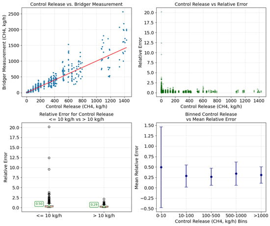
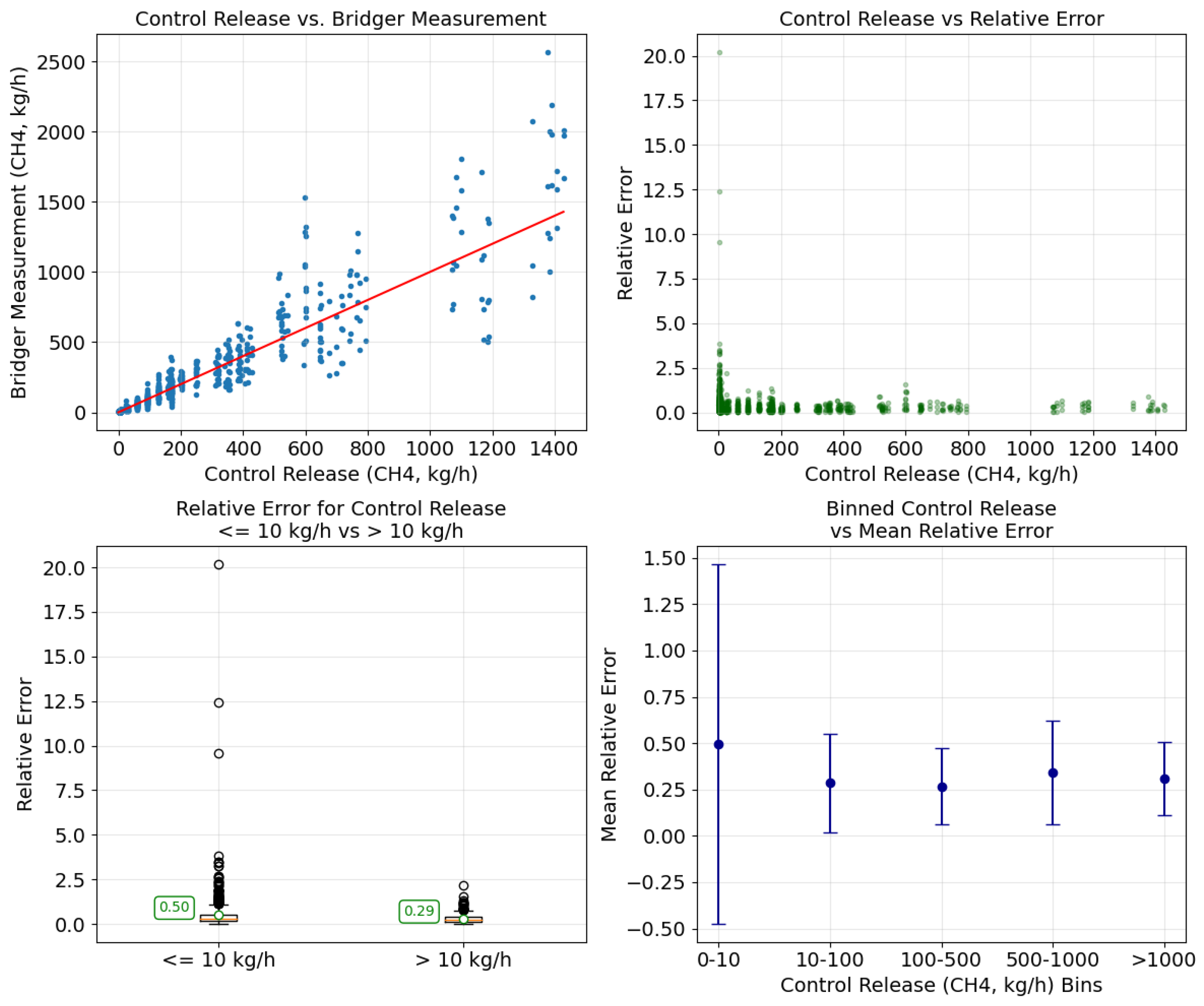
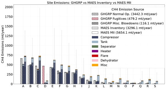
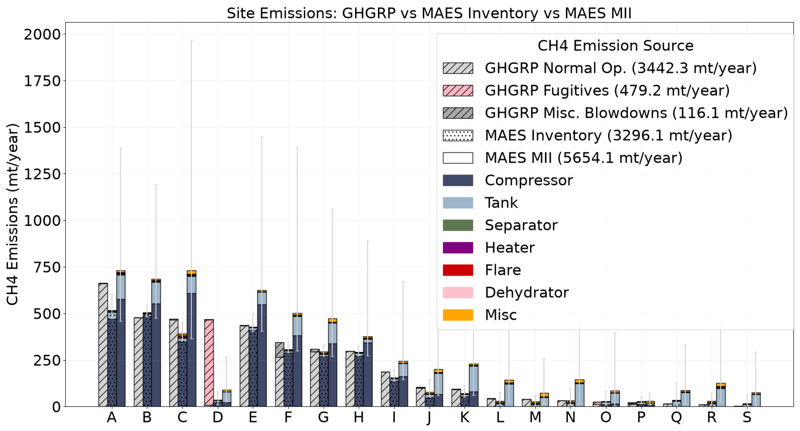
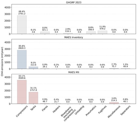
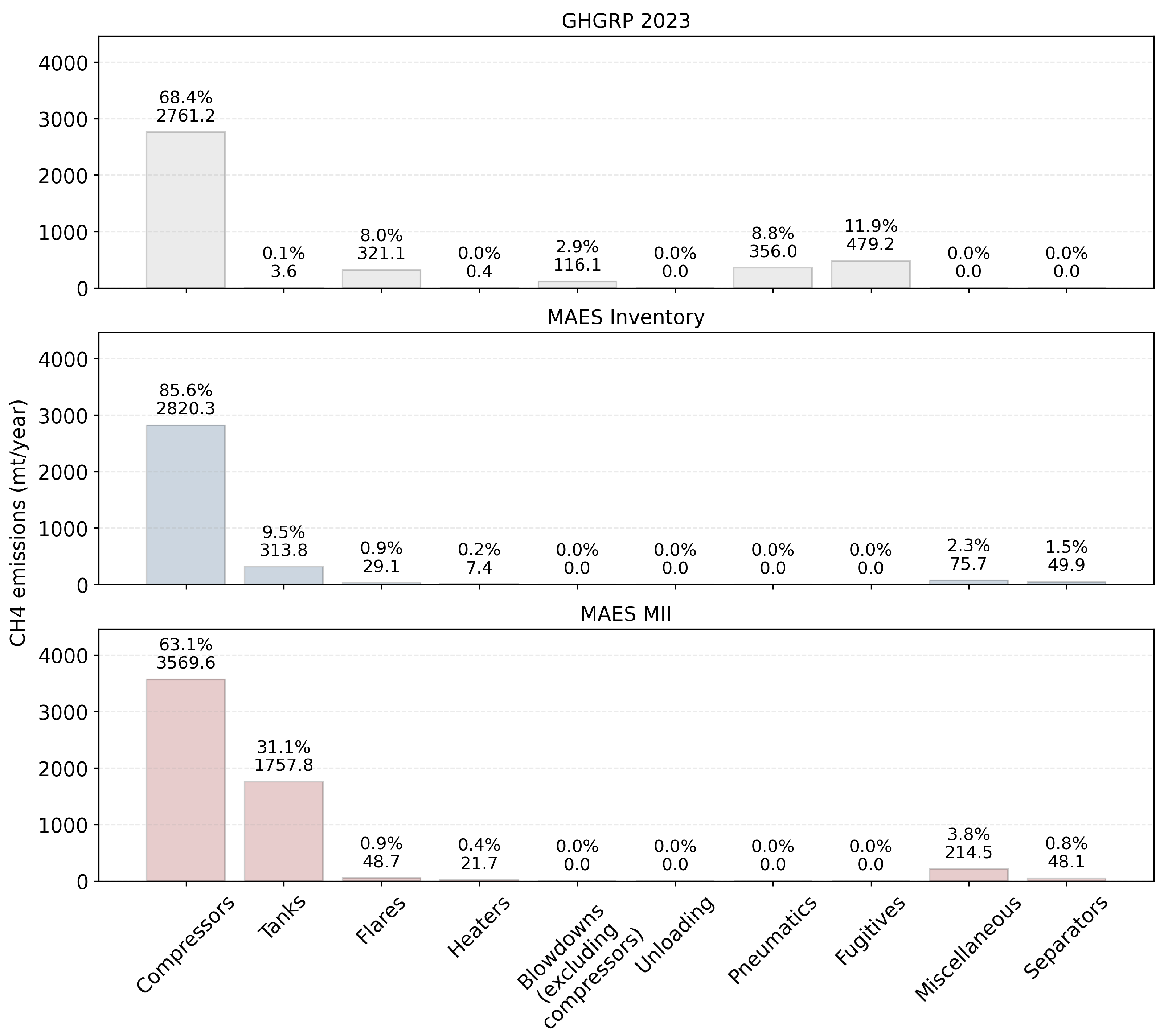
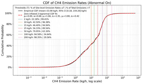
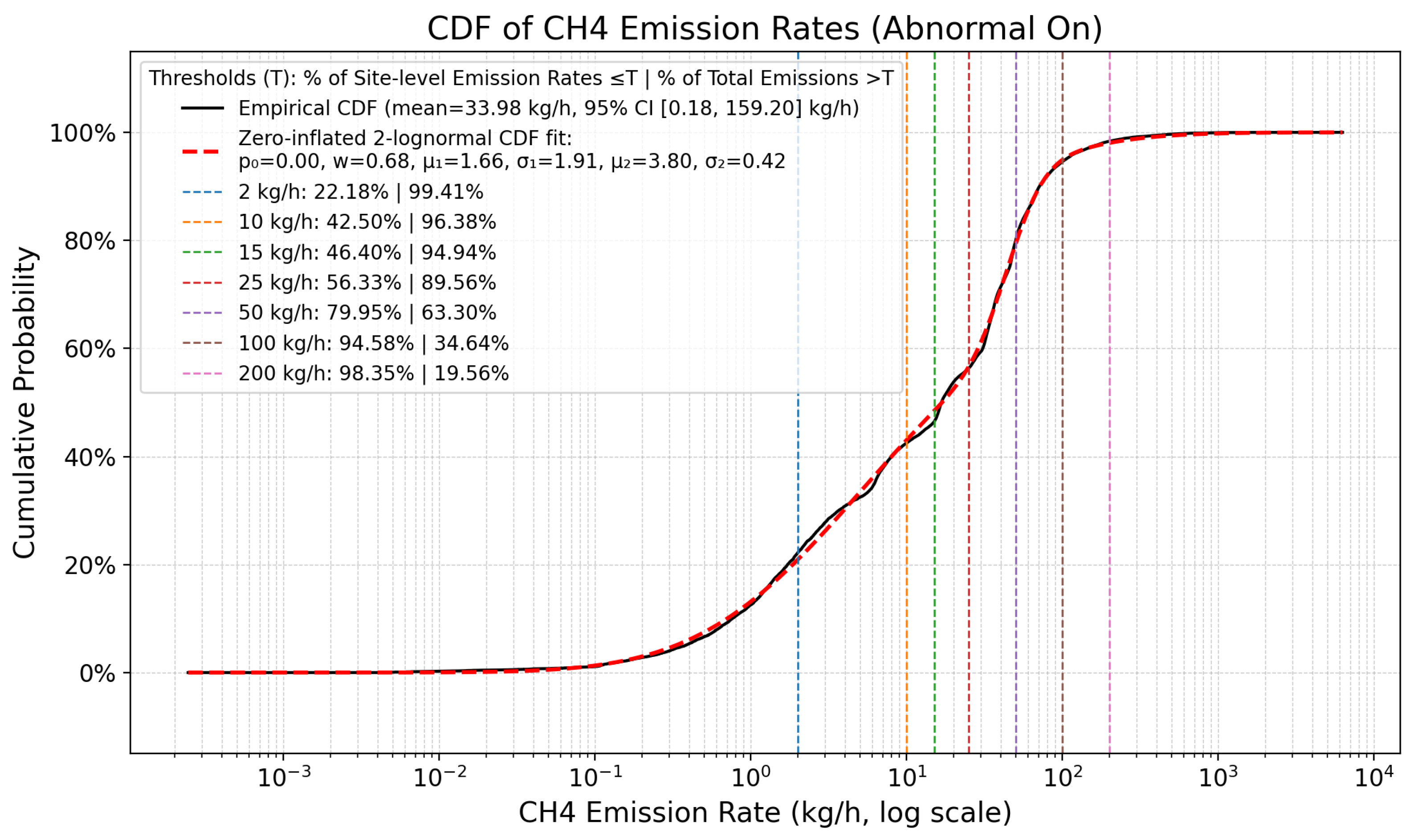

Disclaimer/Publisher’s Note: The statements, opinions and data contained in all publications are solely those of the individual author(s) and contributor(s) and not of MDPI and/or the editor(s). MDPI and/or the editor(s) disclaim responsibility for any injury to people or property resulting from any ideas, methods, instructions or products referred to in the content. |
© 2026 by the authors. Licensee MDPI, Basel, Switzerland. This article is an open access article distributed under the terms and conditions of the Creative Commons Attribution (CC BY) license.