


Abstract
Laterite mining stands out as a relevant, but understudied, form of disturbance in the coastal hinterland of Karnataka, taking place in iron- and aluminum-rich zones in fragile ecosystems as well as agricultural land. This paper discusses the implementation of XGBoost classification and GIS footprint analysis to assess changes in land cover and mining disturbances in Bantwal Taluk (2015–2025) using Landsat 8/9 images and NRSC Level-I classification. The accuracy of cross-validation was 94.4% in 2015 and 90.4% in 2025 (F1 = 0.944 and 0.904), with a decrease due to confusion between the “Barren Land” and “Built-up” classes, leading to a decrease in the F1-score for “Barren Land” from 0.825 to 0.750. The main land-cover changes were the conversion of barren land to agricultural and built-up land, as well as a fourfold increase in the area of water bodies as a result of dam construction. The analysis of footprints showed 71 new and 68 reclaimed sites covering a total area of 3.315 km2 across the two years, that is, 1.8 times the footprint of either year alone, indicating mobile rather than growing mining activity. This XGBoost-GIS approach offers mining authorities a validated, low-cost protocol for tracking similar disturbances and prioritizing monitoring in other coastal, laterite-rich regions.
1. Introduction
Land-cover changes are indicators of interactions between human and natural processes, as well as of how ecosystems provide a variety of services, affect hydrological cycles and carbon fluxes, and stabilize landscapes. Global terrestrial environments are undergoing rapid land transformations due to increased rates of urbanization, agricultural intensification and resource extraction. However, many of these transformations result in irreversible ecological damage if they are not planned or regulated. Consequently, it is essential to understand both the spatial and temporal components of land-cover transition so that effective environmental decision-making and sustainable land-use planning strategies may be developed [1].
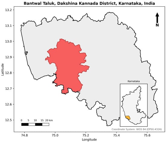
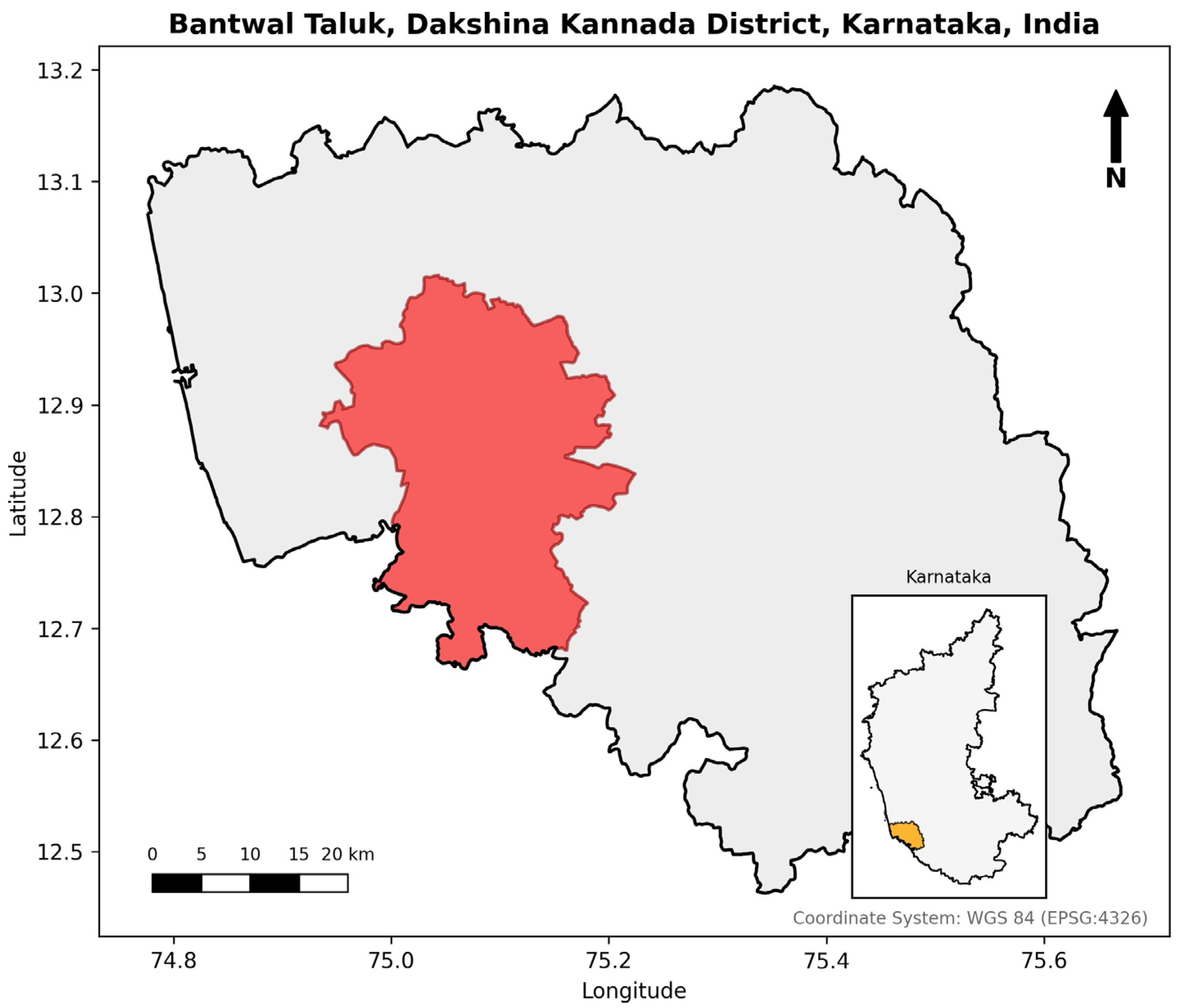
One of the most destructive human land disturbances is mining for minerals, which involves extensive clearing of vegetation and exposure of the soil and underlying substratum [2]. The abundance of laterite deposits in the tropics makes the development of laterite mining a real possibility in these areas. Therefore, the main source of construction materials for buildings and roads is iron- and aluminum-rich laterite deposits [3,4]. Even though laterite mines are mostly small and localized compared to other mineral mining operations (for example, large open pit mines), their cumulative influence on land degradation, hydrologic change and landscape fragmentation can still be significant. However, even though the environmental impacts of laterite mining are well documented, there is a lack of information on this subject in the scientific literature, especially regarding laterite mining and land-cover change at smaller geographical scales, where the effects are supposed to be felt the most pronounced. The lack of information about land-use/land-cover change in South and Southeast Asia is a part of a broader knowledge gap in the field [5]. Dakshina Kannada District, Udupi District and Uttara Kannada District in Karnataka (India) form a narrow band of laterite-capped terrain along the contact zone between the Western Ghats mountain range and the Arabian Sea, within which Figure 1 shows the location of Bantwal Taluk, the focal administrative unit of this study, situated in Dakshina Kannada District, Karnataka.
Figure 1.
Location of Bantwal Taluk within Dakshina Kannada District and Karnataka State, India. Administrative boundaries: © OpenStreetMap contributors.
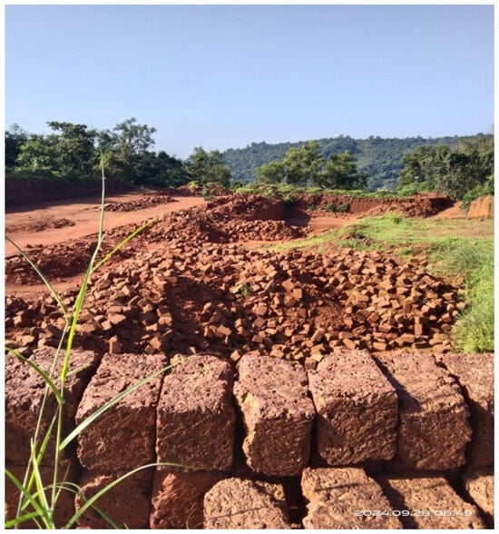
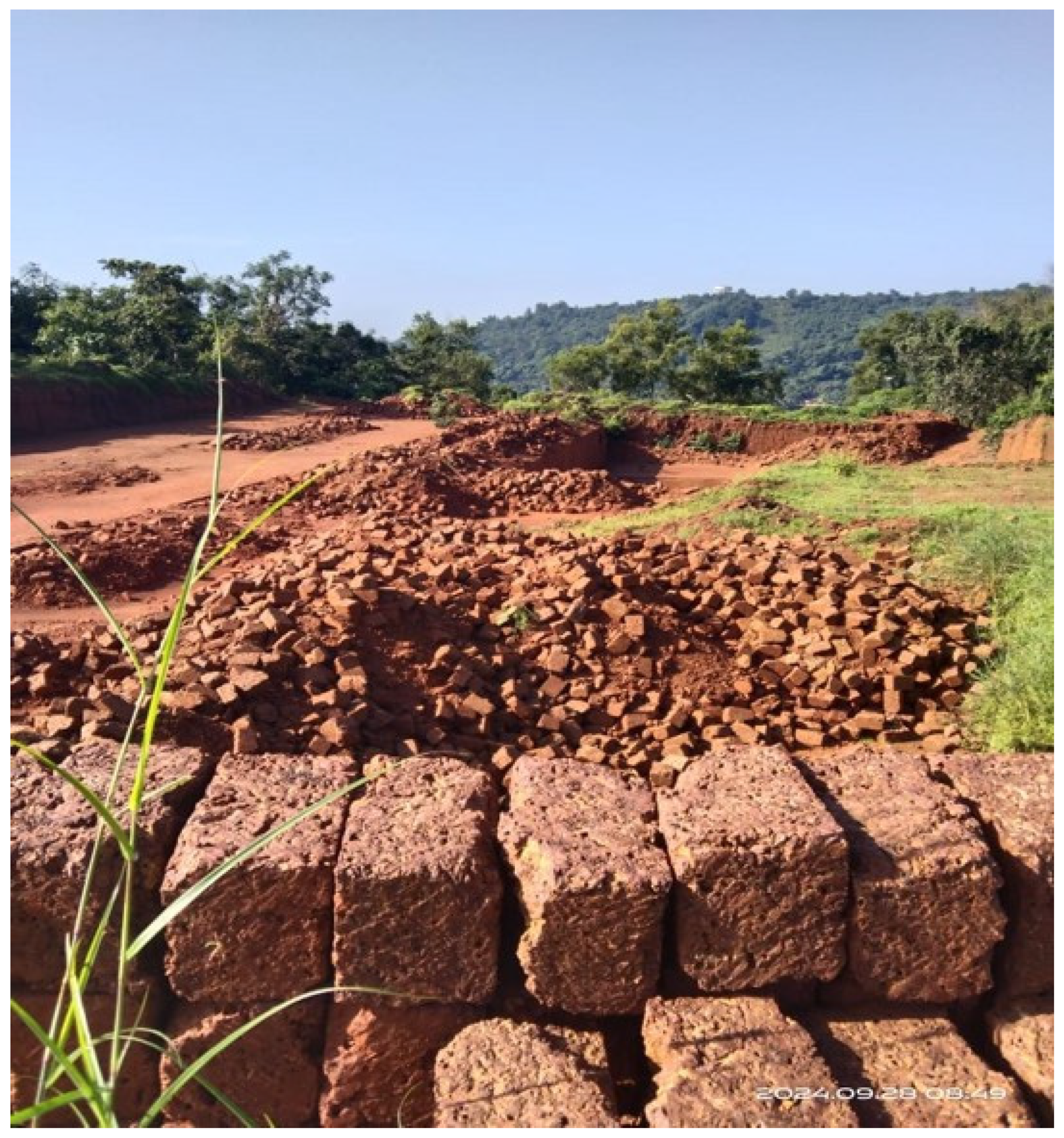
This region consists of a combination of narrow coastal plains, dissected hill systems with upper sections covered in lateritic crusts and lower sections characterized by lithomarge horizons formed during humid tropical climates [6]. Laterite is a type of highly ferruginous and aluminous weathered soil–rock material that is produced from the long-term chemical weathering of basaltic and silicate rock parent materials with subsequent leaching of silica and accumulation of iron and aluminum oxides. This iron and aluminum-rich material is extracted through small-scale, open surface mining, as shown in Figure 2.
Figure 2.
Mining for laterite stones in Bantwal Taluk (photograph captured by the author).
Lateritic profiles are major controls on the patterns of drainage within the region, the distribution of vegetation within the region, the retention of soil moisture within the region and the suitability of land for various uses. All three factors directly contribute to agricultural practices in addition to settlement patterns [7]. Within this geomorphologic setting, laterite mining has become increasingly common within taluk-level administrative divisions such as Bantwal Taluk. For example, the taluk is composed primarily of lateritic uplands that are extensively intermixed with agricultural lands, forest patches and rural residential areas. The extraction of lateritic crusts from this area results in changes to surface roughness, surface runoff generation, groundwater flow within shallow aquifers and increases in soil erosion. Ultimately, these changes will result in a series of long-term ecological and hydrologic consequences. Because many of the impacts caused by this type of mining are both spatially distributed and incrementally variable over time, the detection of these impacts would require either long periods of temporal data collection or remote sensing technology. In this study, this detection is achieved using two representative Landsat scenes, spaced approximately a decade apart (2015 and 2025), enabling decadal change detection rather than continuous multitemporal monitoring. Remote sensing technology offers several advantages related to detecting land-cover change, including efficiency, cost-effectiveness and objectivity. Furthermore, Landsat satellite imagery represents the longest continuously collected dataset of mid-resolution images available globally. Thus, Landsat satellite imagery is uniquely positioned to evaluate environmental phenomena using decadal time scales for assessment purposes. Both Landsat 8 and 9 provide improvements in radiometric sensitivity and signal-to-noise ratio compared to previous generations of satellites and employ identical spectral configurations providing continued consistency and reliability for evaluation purposes. The red, near-infrared (NIR) and short-wave infrared (SWIR) bands are useful in distinguishing between well-vegetated areas, water bodies, and man-made surfaces composed of concrete/asphalt/built-up surfaces/barren areas/mining exposed substrates characteristic of lateritic terrains [1,8]. Nevertheless, there are some limitations to using Landsat data in this case, as continuous cloudiness during the monsoon period might restrict the availability of usable images, while the dry-season period, which is favorable in terms of reducing cloudiness and phenological changes between years, might result in increased spectral similarity between exposed soils and built-up surfaces.
In addition to identifying the appropriate class for each pixel, several methodological challenges must be addressed. Traditional classification methods such as maximum likelihood or rule-based classification perform poorly when applied to landscapes with high spectral heterogeneity. For instance, bare laterite soil, built-up areas, and exposed mining-pit surfaces often exhibit similar spectral signatures, making them difficult to distinguish using conventional methods. Machine learning has therefore become the preferred method for this type of problem, thanks to its capability to model non-linear relationships, handle high-dimensional input and combined spectral characteristics [9]. Of the many options available within machine learning, Random Forest (RF) and Support Vector Machine (SVM) are the two most common. However, in more complex environments such as those created by the mixing of the land covers shown above, Extreme Gradient Boosting (XGBoost 3.4.1.) is being widely adopted [9,10]. XGBoost uses a combination of gradient boosting with regularization to increase accuracy while controlling overfitting and has proven itself to be capable of producing higher accuracies than other traditional or ensemble-based classifiers [10]. Additionally, its ability to include both vegetation indices (e.g., NDVI), built-up indices (e.g., NDBI) and water indices (e.g., NDWI) along with the raw spectral bands provides XGBoost with an advantage when detecting the small-scale variations that result from laterite mining.
Several other studies comparing different classifiers have provided methodological examples to be followed in both India and South Asia. The study by [11] used RF, SVM, Gradient Boosted Trees, and CART with 10 m Sentinel-2 images from Google Earth Engine for land-cover mapping of Jammu District. The study conducted in Cuddalore Taluk, Tamil Nadu, by [12] compared SVM and RF through the application of the NRSC Level-I methodology. Ref. [13] examined the results of SVM, RF, and Maximum Likelihood Classification for land-cover classification of Chennai District. On the African continent, ref. [14] assessed RF, SVM, and XGBoost using Landsat multi-sensor imagery for eThekwini Municipality, South Africa. GEE-based RF classification has also been applied to smaller island settings such as Nadi, Fiji [15].
Remote sensing has been employed to examine the effects of mining on land cover; however, there is a significant bias toward large open pit/coal mines where mined substrate is very apparent relative to the surrounding vegetation [2]. There has been much less interest in small-scale, scattered artisanal mining operations located in humid tropical environments—particularly laterite quarrying [16]. A larger review of mining-related remote sensing literature found that nearly all studies focused on either metalliferous or energy mineral mining and were conducted at high spatial resolutions. Prior evaluations of laterite and hard rock quarrying in the Netravati-Gurpur basin (Bantwal Taluk) relied upon field-based assessment techniques such as questionnaire surveys and slope-based erosion-risk mapping [17], or the Rapid Impact Assessment Matrix (RIAM) [3,18], rather than satellite-derived Land-Use/Land Cover (LULC) classification. While general LULC change assessments exist for the wider Dakshina Kannada District [7], remote sensing-based LULC classification has rarely been combined with laterite-specific mining footprint quantification. Ref. [12] provides the closest precedent to this study, using Landsat imagery (Landsat 4–5 Thematic Mapper and Landsat 8 Operational Land Imager, nominally 30 m spatial resolution) and classifying land cover using a six-class NRSC Level-I scheme that included Mining as an independent class, rather than as a Built-up subclass, as adopted in the present study.
They included a mining class in their NRSC Level-I taxonomy but did not extract mining footprints, perform spatial validations or monitor mining features over time. This appears to be true in general: spatial validations, consensus-based extractions and MMU filtering are rare when mining classes are included in LULC frameworks, limiting how accurately mining dynamics can be assessed at the feature level. In this study, mining is treated as a conceptual subclass of Built-up Land within the NRSC Level-I scheme—reflecting the spectral similarity between the mining substrate and built-up surfaces—and is distinguished from the “mining footprint,” which is the validated, MMU-filtered spatial extent obtained by intersecting the classifier’s Built-up output with manually digitized reference polygons of known mining sites. The objective of this study was to fill this gap for Bantwal Taluk and similar lateritic coastal units in India.
Spectral Indices also contribute here. By combining NDVI, NDBI and NDWI with the main Landsat bands, class separation improves, particularly at the challenging barren–built-up–vegetation boundary defining lateritic mining terrain [9]. Empirical work supports this with measurable increases in accuracy compared to using the Landsat bands independently [19]. This study expands on that by layering the nine-band raster inputs (bands B2–B7 plus NDVI, NDBI and NDWI) for use in an XGBoost model.
Collectively, these gaps indicate the need for four objectives for this study, which are addressed here through an analysis of Bantwal Taluk (approximately 753 km2), Karnataka. The first objective is to develop and test an XGBoost classification framework using multitemporal Landsat 8 (2015) and Landsat 9 (2025) data—obtained from archived satellite acquisitions sourced from the USGS EarthExplorer platform—which are enriched with NDVI, NDBI and NDWI to classify LULC across Bantwal Taluk using the National Remote Sensing Centre (NRSC) Level-I scheme. The second objective is to quantify decadal changes in land cover derived from this classification, focusing specifically on Barren Land, Built-up, Agriculture and Forest. The third objective is to develop a GIS-based methodology for extracting laterite mining footprints from the classified Built-up class, distinguishing persistent, new and reclaimed mining sites. The fourth objective is to quantify the resulting footprint dynamics over the study period, including the total area of mining disturbance across the ten-year period. Together, these four objectives provide an evidence-based and reproducible assessment of both land cover and laterite mining patterns within Bantwal Taluk for the ten-year duration of the study, and are intended to contribute toward the larger goals of tracking land degradation due to small-scale mining and developing more sustainable land-use practices.
2. Materials and Methods
2.1. Study Area
Bantwal Taluk, the study area, spans approximately 753 km2 and is located in Dakshina Kannada District, Karnataka, India, at the transitional geomorphic interface of the Western Ghats escarpment and the Arabian Sea coastal plain. The taluk is characterized by a heterogenous landscape made up of lateritic uplands, agricultural valleys, forest patches and peri-urban settlements and thus constitutes an ecologically sensitive and geologically significant administrative unit. The presence of lateritic geological formations, along with continued demand for construction materials, has made certain areas within this taluk focal points of incremental laterite mining activity, the cumulative disturbance footprint of which has not previously been systematically quantified. The study area boundary was delineated using district-level administrative shapefiles obtained from Survey of India cartographic databases and clipped to the extent of Bantwal Taluk for all analyses.
2.2. Data Acquisition and Selection
Two Landsat Level-1 TP (Terrain Corrected Precision) scenes from Landsat 8 OLI/TIRS and Landsat 9 OLI/TIRS were used to assess the changes in land use over ten years in Bantwal Taluk; a Landsat 8 OLI/TIRS image taken on 5 February 2015 and a Landsat 9 OLI/TIRS image taken on 8 February 2025 (see Table 1). The reason both images were chosen is because they had <1% cloud cover and were taken in the post-monsoon dry season, when vegetation phenology is comparatively stable, minimizing spectral differences between the two years that could otherwise be mistaken for land-cover change. Both images correspond to WRS-2 Path/Row 145/51. Landsat 8 and Landsat 9 were chosen because they provide radiometric continuity that facilitates long-term monitoring [20], and because their OLI instruments are in close radiometric agreement, can be reliably cross-comparable [21], and provide consistent spectral coverage for all three types of bands (visible, near-infrared and short-wave infrared) at 30 m spatial resolution.
Table 1.
Details of Landsat scenes used in the study.
2.3. Data Pre-Processing
2.3.1. Radiometric Calibration and Reflectance Conversion
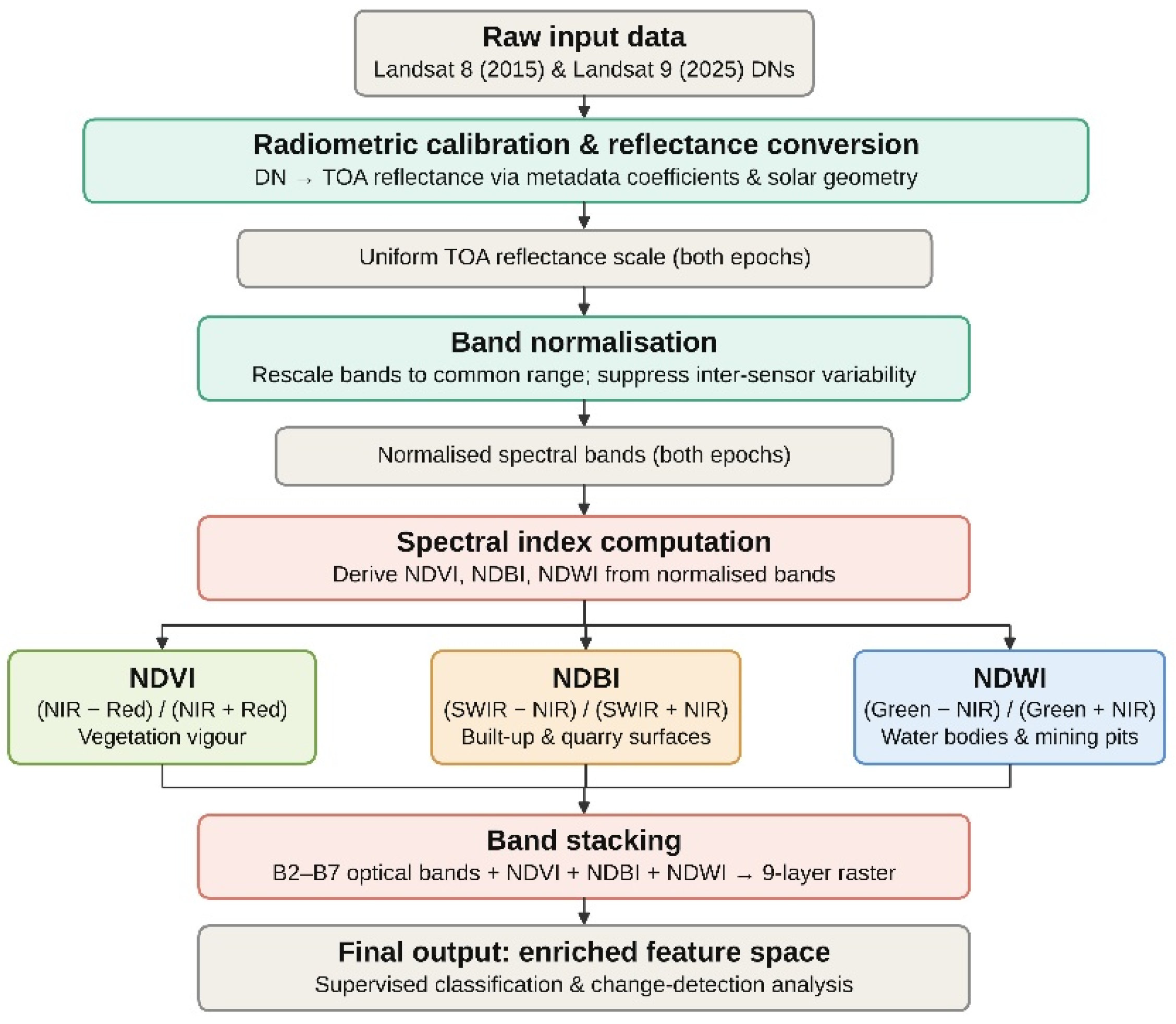
In order to perform a radiometrically consistent data comparison between sensors and epochs, raw DNs observed from reflective bands of Landsat 8 in 2015 and Landsat 9 in 2025 were rescaled into TOA reflectance using rescaling coefficients and solar angles provided within scene metadata. While the instruments have some design continuity, the comparison of raw DNs can cause systematic errors due to slight differences in sensor calibration and geometry of observations—e.g., solar elevation angles of 49.53° and 50.29°, and solar azimuth angles of 135.01° and 133.76°, respectively. The conversion of both datasets to TOA reflectance made it possible to use a common radiometric scale and to conduct a spectrally meaningful comparison over the decade. Surface reflectance data products that include atmospheric correction have not been used in this research. While surface reflectance is generally preferable for multitemporal change detection due to its higher atmospheric correction accuracy [22], TOA reflectance data were deemed sufficient for this study, as the scenes were taken under very similar atmospheric conditions during the dry season with low cloud cover (<1%); this trade-off is discussed further in Section 4.4.
2.3.2. Band Normalization
In order to remove the sensor variability, each band (B2–B7) was normalized to a standard reflectance range of 0 to 1 using linear min–max normalization (Equation (1)), applied separately per band and per year:
where Bandmin and Bandmax represent the minimum and maximum observed values of that band within the corresponding scene. This step was very beneficial for the mining analysis at a taluk scale since small changes in spectral characteristics of vegetation and bare ground compared to the mined materials could be mistaken for land-cover change.
2.3.3. Spectral Index Computation
To improve separability and provide more discriminative classification, three spectral indices were generated from normalized bands. The Normalized Difference Vegetation Index (NDVI) was generated to assess vegetative health and density, and to separate intact vegetation from degraded or cleared areas near mines (Equation (2)):
The Normalized Difference Built-up Index (NDBI) was developed to detect built-up and impervious surface cover associated with urban development and mine infrastructure (Equation (3)):
The Normalized Difference Water Index (NDWI) was employed to identify permanent and perennial waterbodies, including those found at dams, reservoirs, and seasonal water-filled mining-pit depressions (Equation (4)):
Since the imagery was collected during the dry season (February), NDWI was generally able to detect permanent hydrologic features and exclude temporary accumulation of water.
2.3.4. Band Stacking
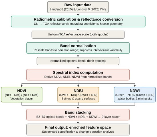
The normalized and spectrally indexed optical bands (B2–B7; Blue, Green, Red, Near-Infrared, Short-Wave Infrared-1, and Short-Wave Infrared-2) along with the derived spectral indices (NDVI, NDBI, NDWI), were then integrated into a singular nine-layer raster for each epoch to create an optical and spectrally enhanced feature space that is designed to provide maximum separation between classes for robust supervised classification and further support for change detection. The entire data pre-processing workflow is illustrated in Figure 3.
Figure 3.
Workflow of data pre-processing.
2.4. Training Data Preparation
The training sample was developed using Google Earth Pro (version 7.3) by manually digitizing very high-resolution images. The attributes from the digitized layers were then integrated into an attribute schema. Reference polygons were drawn to represent spectrally homogeneous land-cover parcels in Bantwal Taluk. The NRSC Level-I land-cover classification scheme was used to assign class codes and distinguishes seven broad categories, namely, Built-up Land, Agriculture, Forest, Grass/Grazing, Barren/Unculturable/Wasteland, Wetlands/Water Bodies, and Snow.
For the purpose of the analysis, five Level-I classes were retained: Built-up Land, Agriculture, Forest, Barren Land and Water Bodies. The Grass/Grazing class was excluded because of the lack of representative samples in the study area, and the Snow class was excluded due to its natural absence in the humid tropical setting. Invalid geometries were filtered out and the shapefiles were reprojected to the Landsat imagery UTM Zone 43N coordinate system. Spectral values were extracted for each polygon from the pre-processed nine-band raster stack. The 2015 and 2025 data sets were sampled independently using the same sampling procedures, to make the classification results temporally comparable.
The number of manually delineated training polygons for the five selected land-cover types in 2015 and 2025 amounted to 248 and 140 polygons, respectively (78/53/50/41/26 for Built-up, Agriculture, Forest, Barren Land, and Water Bodies in 2015, and 59/22/24/15/20 in 2025). Polygons had sizes ranging from 13.6 to 178,917.1 m2. No minimum threshold for polygon size was set during the digitization process; polygons were instead delineated using the visual boundaries of each homogeneous spectral patch in the reference images. It is necessary to mention that one-third of polygons (33%) in 2015 and almost one-quarter in 2025 (22%) are smaller than a Landsat pixel (900 m2). Training polygons were distributed across the spatial extent of the study area for both years (2015 and 2025), without deliberate geographic clustering. Polygons were selected through visual inspection of the reference imagery for spectrally homogeneous areas. In other words, no stratified sampling method was used to ensure representation of the spectral heterogeneity of the study area. Since both the land-cover training polygons and the mining reference polygons (Section 2.8) have been digitized using high-resolution imagery from Google Earth Pro, their analysis relative to the classified raster at 30 m is subject to positional accuracy issues due to the difference in resolution; this is discussed further in Section 3.4.
2.5. Land-Cover Classification Using XGBoost
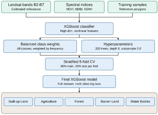
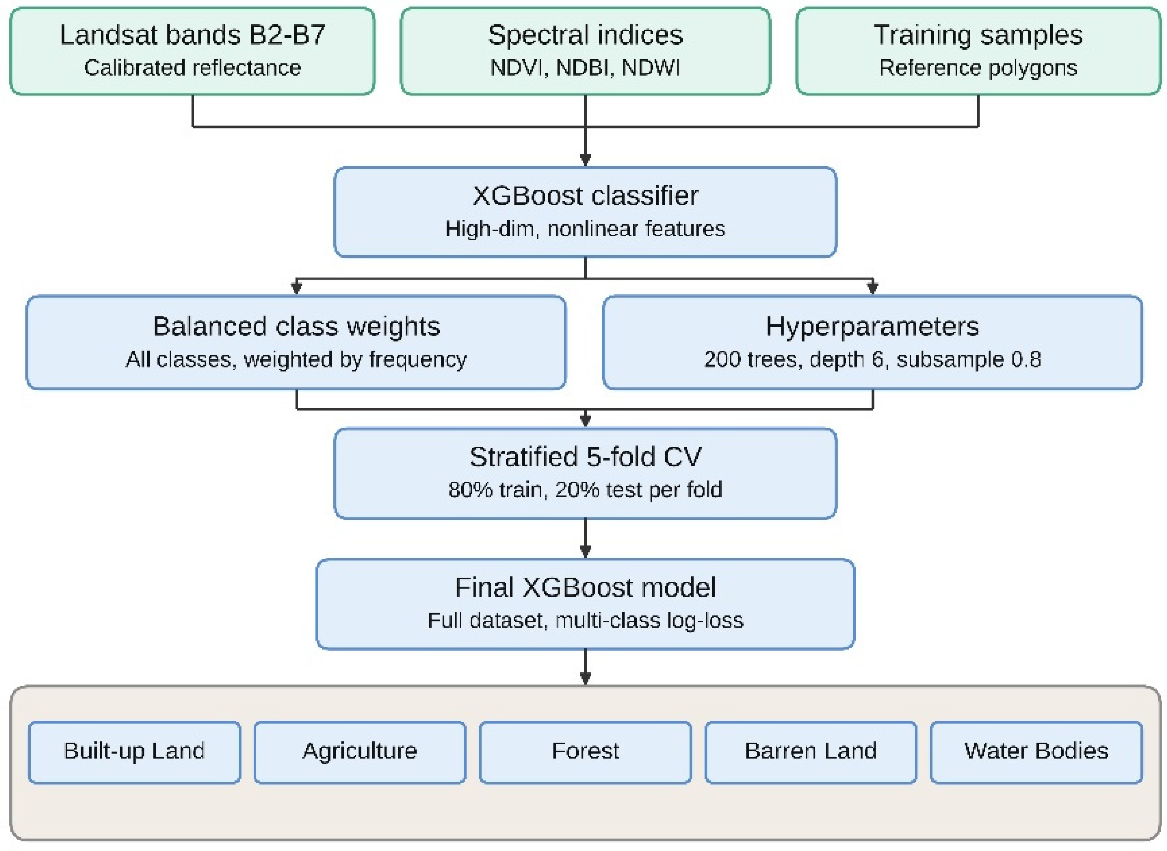
In order to perform the land-cover classification, an XGBoost machine learning model was developed using the calibrated Landsat bands (B2–B7) and three additional derived spectral indices (NDVI, NDBI, NDWI). Cross-validation folds were constructed at the pixel level using the stratified k-fold method; further detail on the cross-validation procedure is provided in Section 2.6. The final classification model was trained on the full dataset with n = 200 gradient boosted trees, a maximum tree depth of 6, a subsampling rate of 0.8, and a column sampling rate of 0.8. No formal hyperparameter optimization technique, such as grid or random search, was applied to this study’s dataset; therefore, the hyperparameters were selected from ranges found in previous XGBoost tuning studies (for example, Ref. [23] for n_estimators and max_depth), with default regularization levels (subsample and column sampling) to limit the risk of overfitting. Class weights for the training phase were balanced using weights inversely proportional to class frequency, to provide equal representation for the minority classes (water bodies and Barren Land), consistent with recommended practice [24] when applying tree-building methods to unbalanced classification problems. The optimization criterion was the multiclass log-loss function, which is widely recognized as the most suitable choice for multiclass probabilistic classification. Spatial predictions were produced in a memory-efficient, batch-by-batch manner, with each pixel classified into one of the five NRSC Level-I classes. Training of the land-cover classification model was carried out in Python 3.12 using the XGBoost and scikit-learn modules, running in Google Colab, while QGIS 4.2.3. was used for spatial data visualization and map generation. The entire land-cover classification procedure is illustrated in Figure 4.
Figure 4.
Methodological steps in land-cover classification with XGBoost.
2.6. Accuracy Assessment
Model evaluation was performed using stratified 5-fold cross-validation to keep the class ratio consistent in each fold. In each fold, 80% of the data samples were retained for training and the remaining 20% were left for testing, such that all samples were used in both training and testing across the five folds. Confusion matrices were created from each fold’s held-out data and averaged across the five folds to produce a single representative confusion matrix per epoch. Based on this average confusion matrix, Precision (Equation (5)), Recall (Equation (6)), Specificity (Equation (7)), F1-score (Equation (8)), and Intersection-over-Union (IoU) (Equation (9)) per class were calculated as:
where TP, FP, FN, and TN denote true positives, false positives, false negatives, and true negatives for each class, respectively, derived from the averaged confusion matrix. Class-wise metrics were combined into an overall weighted average, weighted by class sample size, to summarize classifier performance across majority and minority classes. The averaged confusion matrix for each epoch was also used to identify sources of misclassification between classes. These metrics jointly provide strong evidence for model generalization ability and the reliability of the final land-cover maps.
2.7. Post-Classification Change Detection
Change in land cover between 2015 and 2025 was assessed using a post-classification approach, in which two independently classified rasters (2015 and 2025) were compared pixel by pixel. Each pixel in both rasters had two class attributes—one for 2015 and one for 2025—forming a “from-to” class pair. The total area (km2) of each class pair was computed to populate a five-by-five transition matrix, where diagonal values represent unchanged classes and off-diagonal values represent changed classes.
2.8. Mining Footprint Extraction and Consensus Analysis
Consensus mining regions were derived by intersecting the classified Built-up class with mining site polygons, consistent with the NRSC Level-I/II classification scheme, in which mining is treated as a subclass of Built-up Land. Reference mining polygons were obtained by visually interpreting Google Earth Pro imagery and were aligned to the raster coordinate system to ensure geometric consistency with classification outputs; the topological validity of all the reference geometries was verified prior to analysis.
Two consensus mining layers were created for each epoch: (i) a raw consensus layer that contains all intersected features with no minimum mapping unit (MMU) constraints, and (ii) an MMU-filtered consensus layer that contains only features with an area of ≥3600 m2, or four Landsat pixels, to remove isolated, sub-pixel false detections. Consensus-layer construction and MMU filtering were performed in Python using the GeoPandas library. Because the Consensus Layer is constructed as a polygon that intersects each Reference Mining Polygon, it cannot, by definition, cover any area outside those polygons. The resulting recall measurement therefore represents the percentage of the Reference Mining Area correctly recovered by the classification within the Built-up class; it does not test the model’s ability to independently identify mining activity elsewhere across the landscape.
3. Results
3.1. Classification Results: 2015
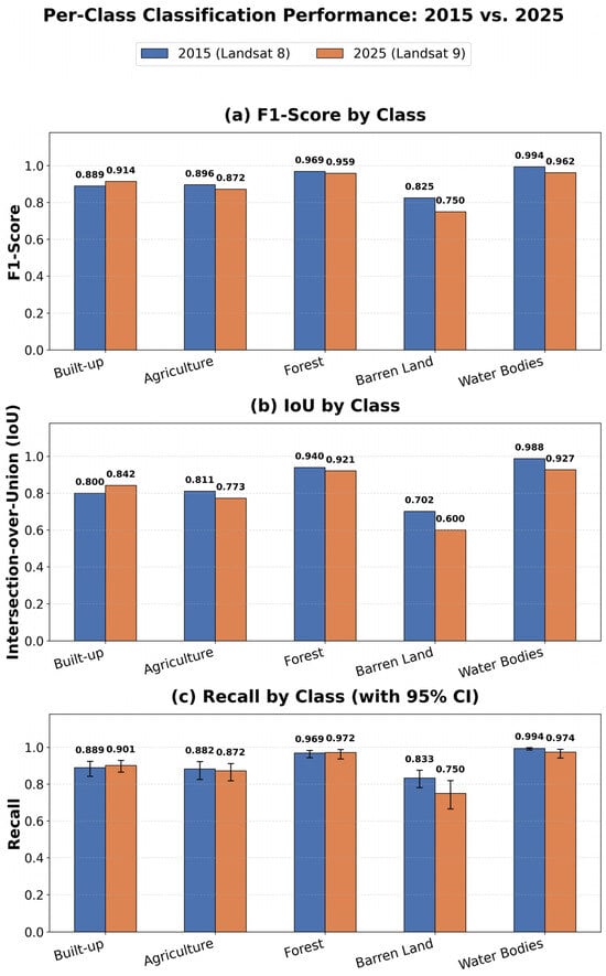
The XGBoost classifier successfully used the 2015 Landsat 8 imagery for all five folds of cross-validation, achieving an overall accuracy of 94.43% and a weighted F1-score of 0.944 (Table 2). A mean IoU value of 0.848 was also achieved across all classes, signifying that there is good spatial correlation between the predicted and actual boundaries of different land-cover types. With respect to individual classes, Water Bodies demonstrated both the highest class-wise F1 scores (F1 = 0.994) and IoU values (IoU = 0.988); similarly, Forests had high class-wise F1 scores (F1 = 0.969) and high class-wise IoU values (IoU = 0.940). Conversely, lower than average F1 and IoU values were observed for Built-up Land (F1 = 0.889; IoU = 0.800) and Agricultural Land (F1 = 0.896; IoU = 0.811), with the latter being the most confused with other classes as a result of similarities in their spectral characteristics.
Table 2.
Per-class accuracy metrics for 2015 (Landsat 8), averaged across five-fold cross-validation.
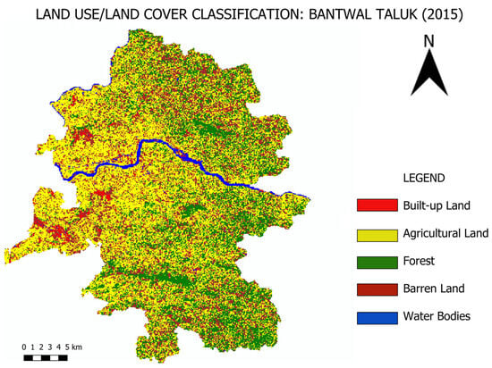
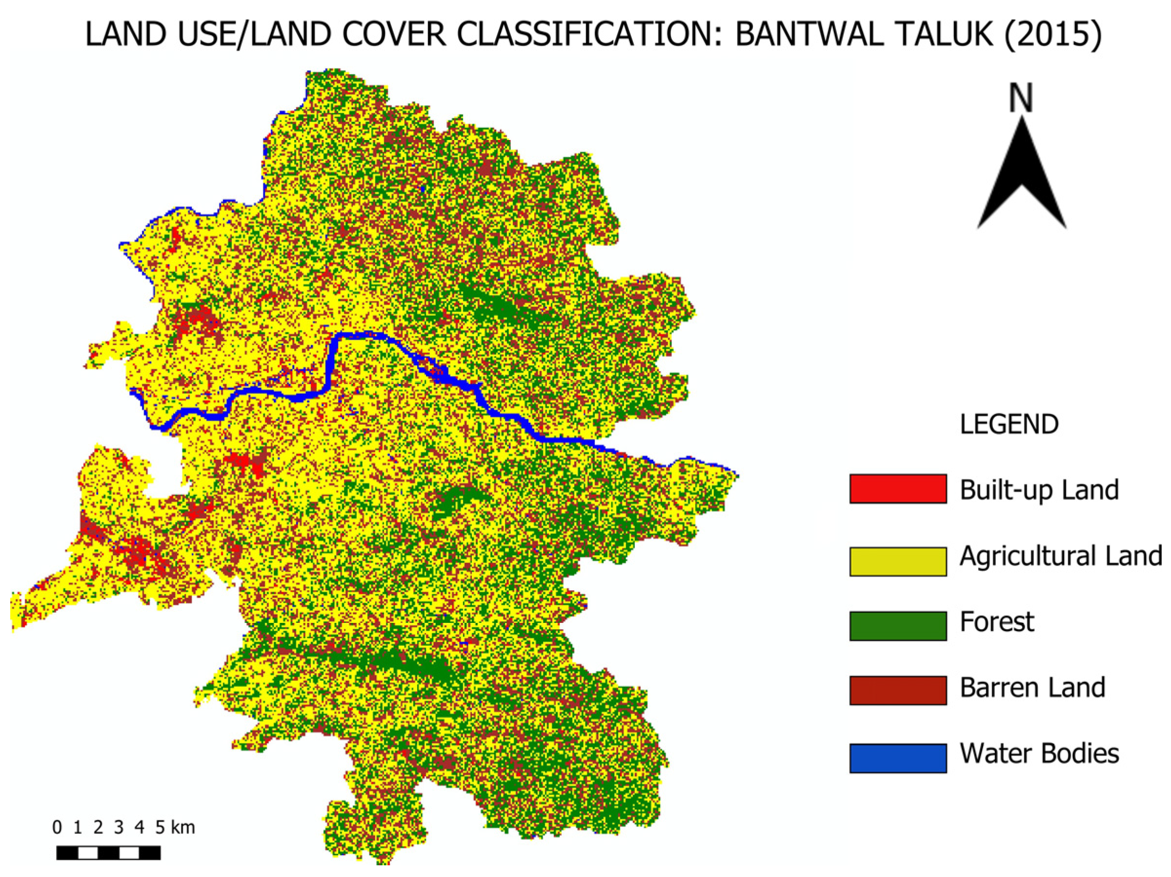
Confidence intervals of 95% were computed for overall accuracy and per-class recall using the Wilson score method, based on the total number of validation samples per class. The confidence interval for overall accuracy was [93.27%, 95.40%]; per-class recall intervals were narrower for classes with larger sample sizes (e.g., Water Bodies, n = 837) and wider for smaller classes (e.g., Agriculture, n = 173). It has been observed that the proportion of training samples for each class is not proportional to its share of the total mapped area (for example, Water Bodies formed less than 2% of the total mapped area in 2015, but accounted for 46% of the training samples). This is because of the nature of the sampling method, where the number of samples depends on the size and number of polygons rather than being area-proportional; Water Bodies comprise few but large, homogeneous polygons and therefore yield more pixels per polygon compared to classes such as Agriculture, which are represented by more numerous, smaller, and more fragmented parcels. Figure 5 shows the LULC map for the 2015 classification.
Figure 5.
Land-Use/Land Cover map of the 2015 classification.
3.2. Land-Cover Classification: 2025
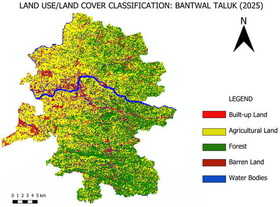
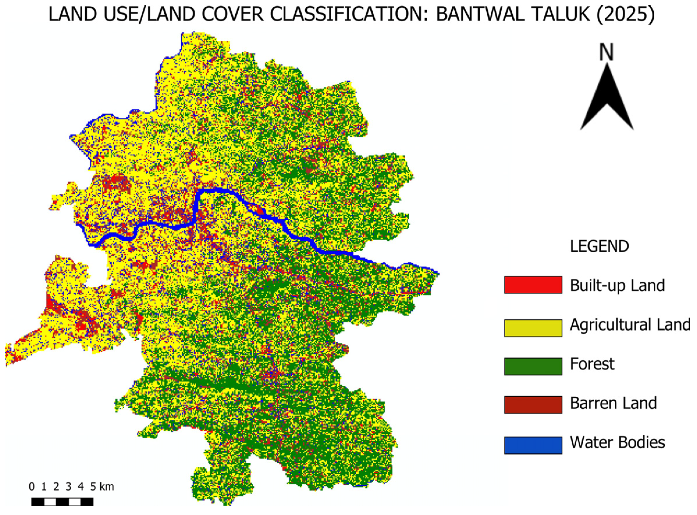
A 2025 classification using the Landsat 9 data resulted in an overall accuracy of 90.43% and a weighted F1 score of 0.904 (Table 3). In addition, there was an average IoU of 0.813 for all classes. When compared to 2015, there was a slight decrease in overall accuracy (4.00 percentage points). This is largely due to Barren Land, as it showed the largest decrease in the F1 score of any class because of the increased spectral overlap between Barren Land and Built-up land-use types. A secondary reason for this decrease in overall accuracy is related to Water Bodies, which had a smaller F1 score in 2025 than in 2015 (F1: 0.994 vs. 0.962). Moreover, although Built-up Land was trained on many more samples (n = 353 in 2025 vs. n = 230 in 2015), it performed better in classification (F1: 0.914 in 2025 vs. 0.889 in 2015). As with previous years, Forest remains one of the best classified classes (F1 = 0.959; IoU = 0.921), along with Water Bodies (F1 = 0.962; IoU = 0.927), even though the latter showed a reduction in classification performance compared to earlier years. The 95% confidence interval for overall accuracy in 2025 was [88.50%, 92.07%]. Consistent with 2015, per-class recall intervals were wider for classes with smaller sample sizes, notably, Barren Land (66.6–81.9%, n = 120). Figure 6 shows the Land Use Land Cover map of the 2025 classification. As in 2015 (Section 3.1), training sample proportions in 2025 do not match each class’s share of the total mapped area, reflecting the same polygon-based sampling characteristics.
Table 3.
Per-class accuracy metrics for 2025 (Landsat 9), averaged across five-fold cross-validation.
Figure 6.
Land-Use Land Cover map of the 2025 classification.
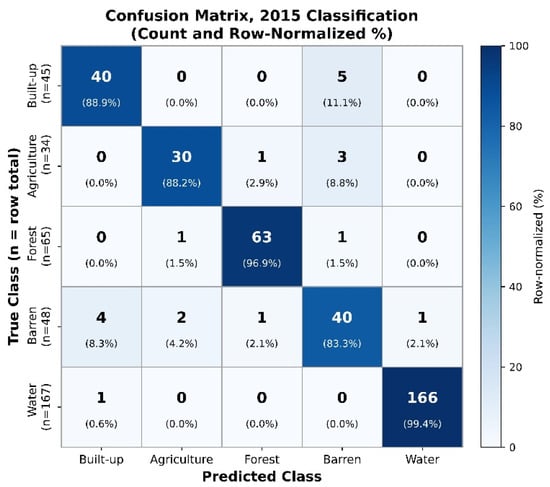
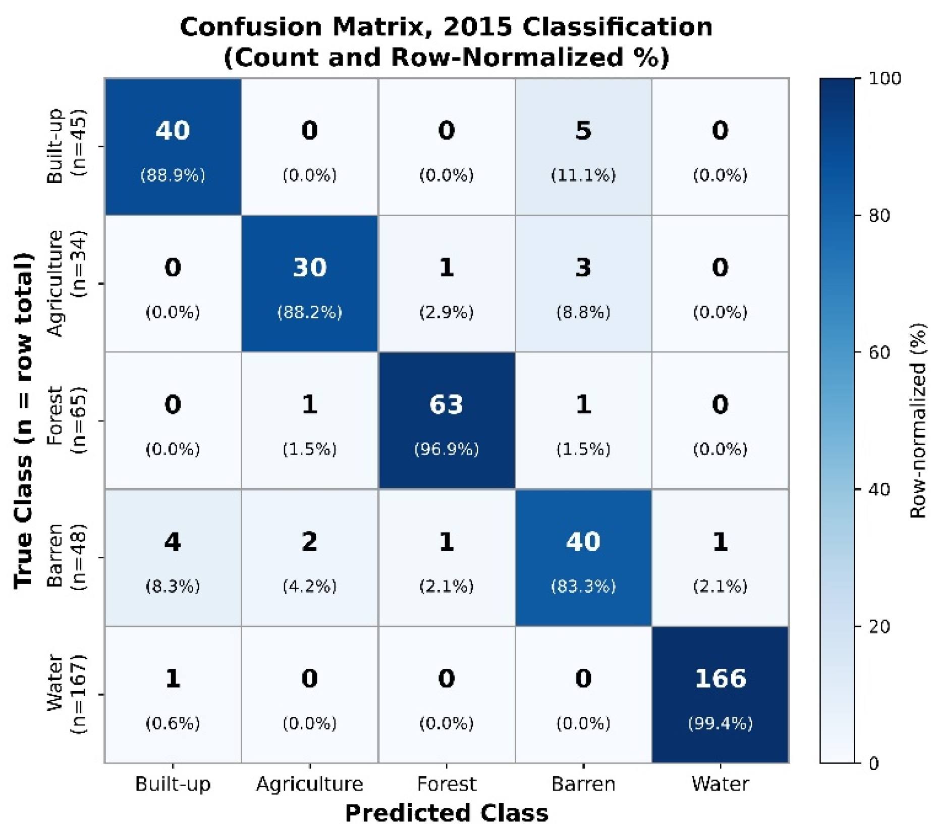
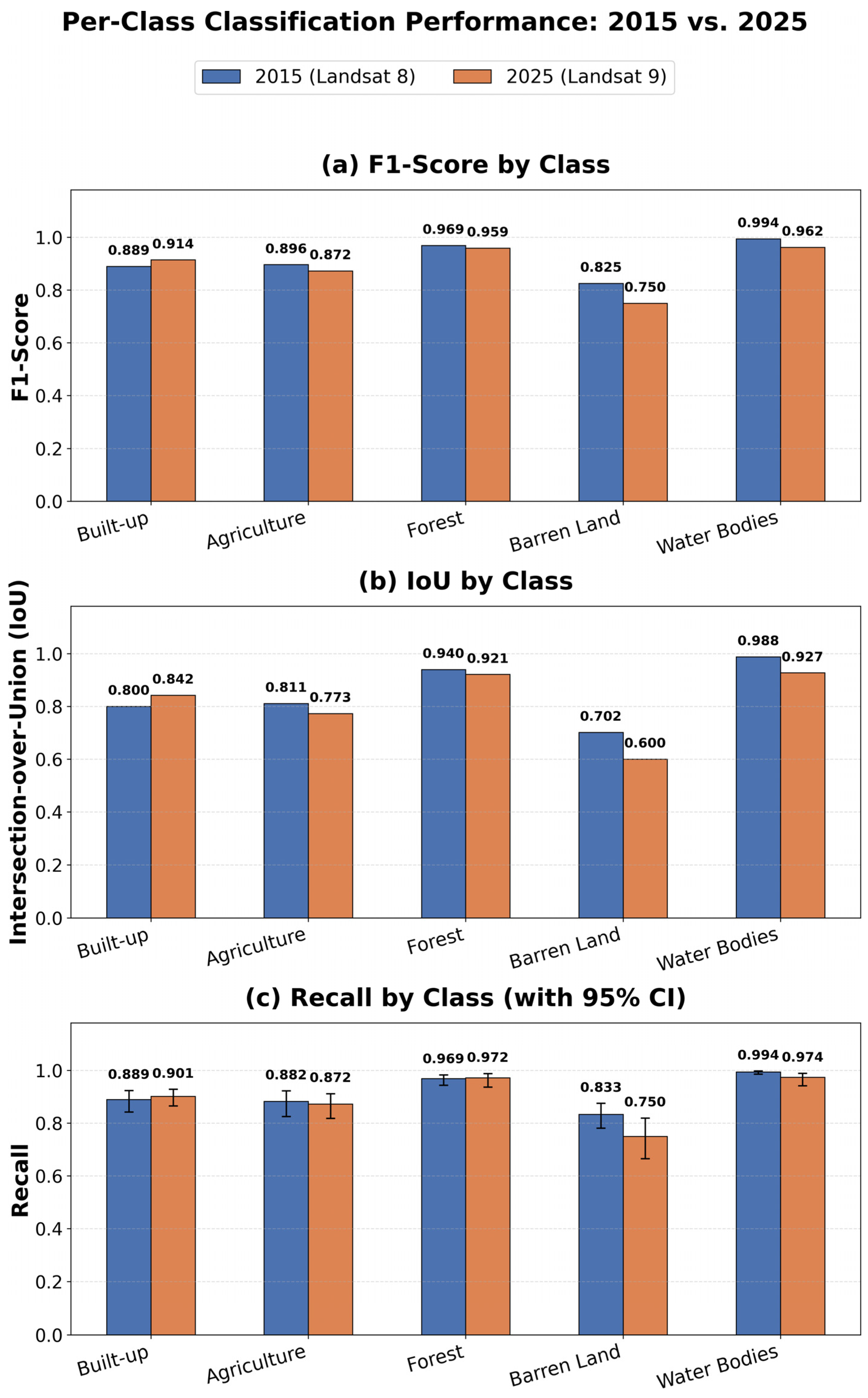
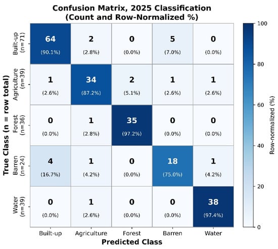
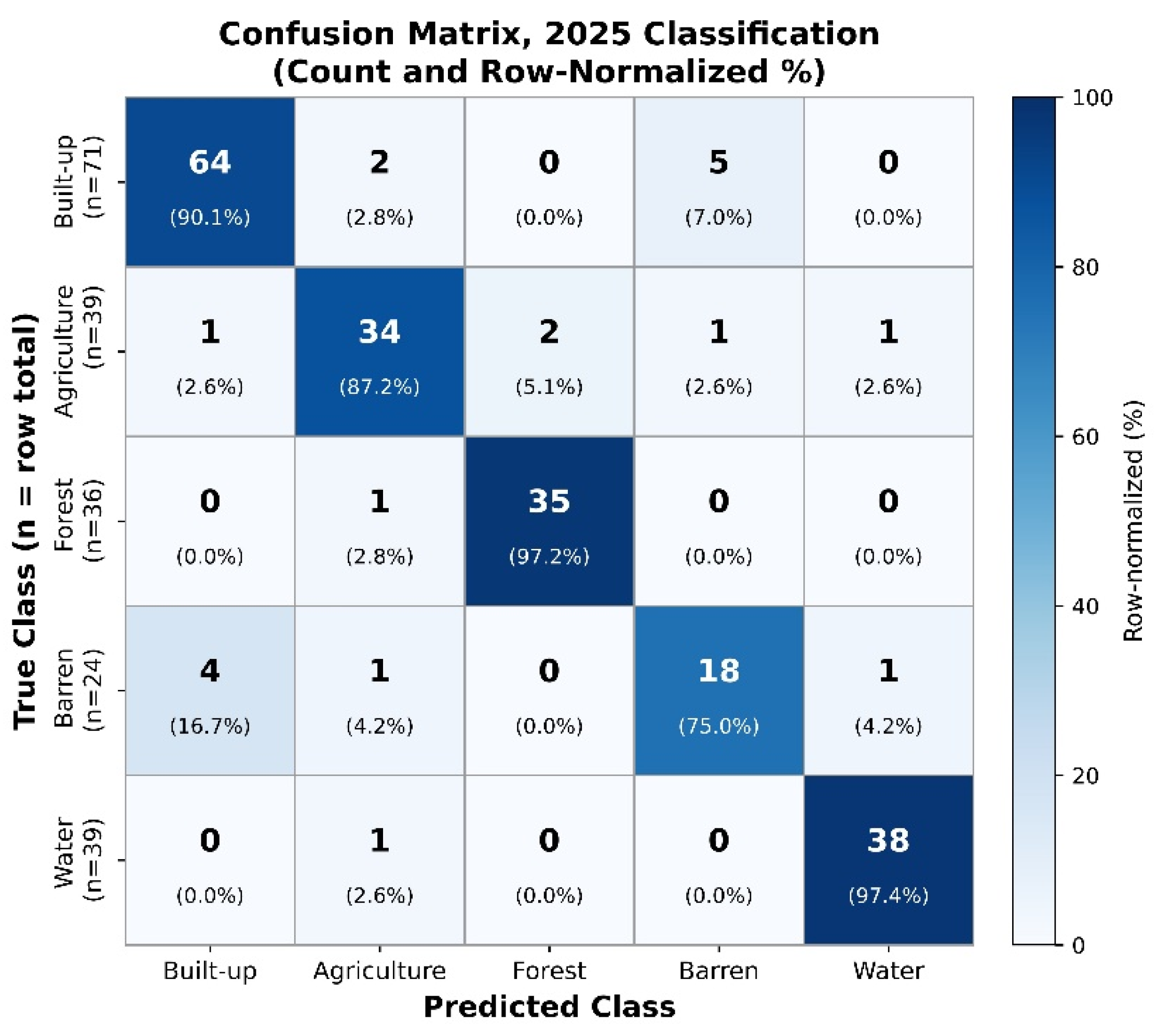
The row-normalized confusion matrices for both epochs (Figure 7 and Figure 8) show the percentage of each true class predicted as each class, averaged across the five cross-validation folds. Further Figure 9 visualizes the per class F1 score, IoU, and Recall values reported in Table 2 and Table 3, with 95% confidence intervals shown for Recall Values of the confusion matrix represent the test portion of the cross-validation folds and hence constitute a subset of the total number of samples used in Table 2 and Table 3.
Figure 7.
Confusion matrix for the 2015 land-cover classification, averaged across five-fold cross-validation. Each cell shows the raw sample count (top) and row-normalized percentage (bottom); row labels indicate the total samples (n) per true class.
Figure 8.
Per-class F1-score, IoU, and Recall (with 95% confidence intervals) comparison between 2015 and 2025.
Figure 9.
Confusion matrix for the 2025 land-cover classification, averaged across five-fold cross-validation. Each cell shows the raw sample count (top) and row-normalized percentage (bottom); row labels indicate total samples (n) per true class.
3.3. Post-Classification Change Detection (2015–2025)
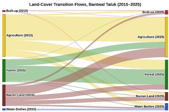
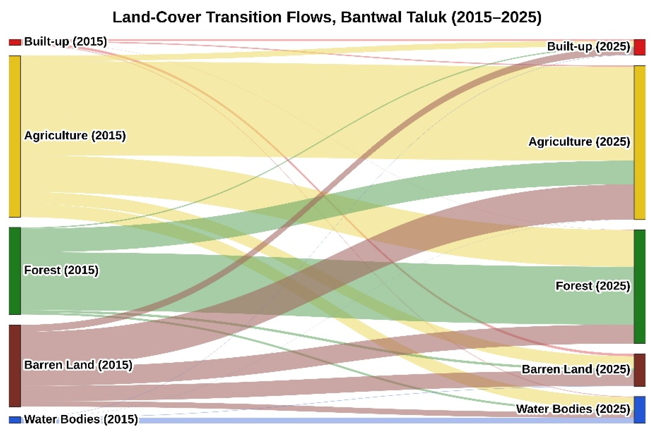
Post-classification change detection has revealed significant changes in land cover in Bantwal Taluk during the period 2015–2025 (see Table 4). Of all the land covers examined, barren land experienced the largest decline, with an area reduction of −108.53 km2 from 179.68 km2 to 71.15 km2; these reductions were largely due to conversion to agriculture (77.17 km2), forest (41.52 km2), and built-up areas (15.37 km2). Thus, much of this area was subjected to both land restoration and continuing expansion for urbanization. Built-up land expanded to almost three times its size prior to 2015, i.e., +21.70 km2 from 13.31 km2 to 35.01 km2. Forest expanded significantly, from 191.25 km2 to 249.65 km2 (+58.39 km2); this increase was mainly due to the conversion of agricultural land (80.62 km2) and barren land (41.52 km2), while there was also some loss of forest to agricultural land (51.98 km2). The area of water bodies increased substantially from 13.86 km2 to 58.69 km2 (+44.82 km2), which is attributable to the construction of dams and barrages in the region during the study period, as elaborated further in Section 4.2; 11.90 km2 of the total water body in 2015 remained unchanged. Finally, although agriculture declined slightly over time, i.e., −16.39 km2, it still retained 206.59 km2 of its original area and is thus experiencing some level of stability. This net decrease occurred because Agriculture’s substantial gains from Barren Land (77.17 km2) and Forest (51.98 km2) were outweighed by its combined losses to Forest (80.62 km2), Water Bodies (28.79 km2), Barren Land (26.47 km2), and Built-up (12.54 km2). The changes in land cover from 2015 to 2025 have been represented by a Sankey Diagram (see Figure 10) illustrating the relative size of each transition. As shown in this diagram, persistence (the area that remains in the same category) has been left out so that only transitions between different land-cover classes are highlighted. The full set of transitional data can be seen in Table 4.
Table 4.
Land-cover transition matrix (2015–2025), area in km2.
Figure 10.
Land-Cover Transition Flows, Bantwal Taluk (2015–2025). In this diagram, flow color represents the 2015 class and flow width is proportional to the transitional area (in km2). Persistence flows (that is, flows where an area remains in its original class) have been left out to improve readability. Please refer to Table 4 for the complete transitional matrix, with all persistence included.
3.4. Laterite Mining Footprint Analysis
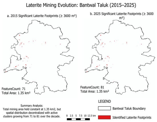
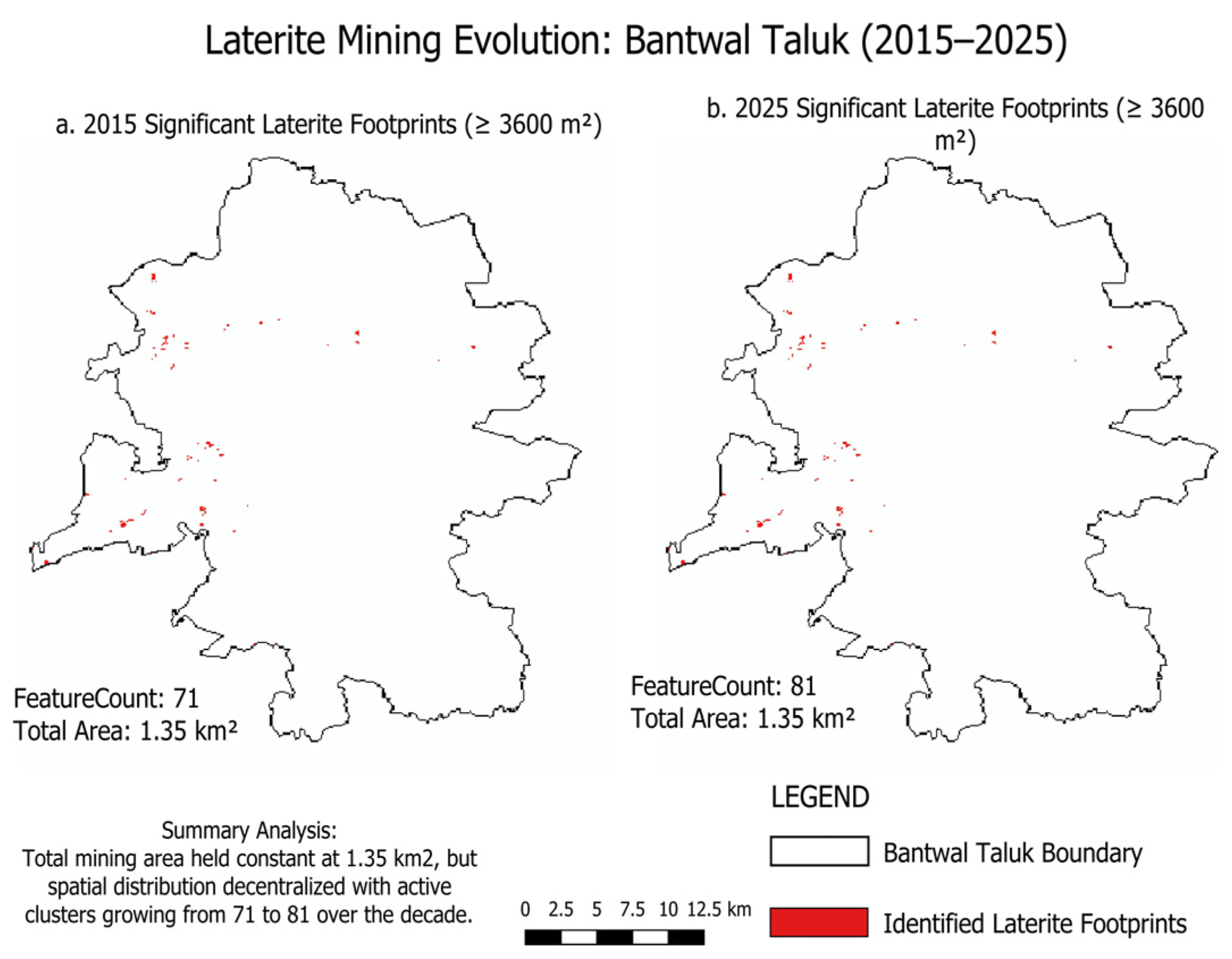
Figure 11 depicts the spatial distribution of validated mining footprints across the taluk in 2015 and 2025, respectively, and also illustrates the decentralization trend discussed in the following sections. Given that mining substrate is categorized under the Built-up class under the NRSC Level-I protocol, mining locations have been considered as one of the elements represented under the category of Built-up. The IoU obtained from the classification of the Built-up class (0.800 in 2015; 0.842 in 2025) is therefore partly influenced by the spatial agreement of the boundaries of mining sites in the reference layer to that of the classified raster. A consistent positional buffer (e.g., ±15 m) was not applied before intersecting with the mining reference layer, as doing so may incorporate other non-mining Built-up elements into the consensus layer, potentially reducing false negatives at the boundary while introducing new false positives.
Figure 11.
Laterite mining footprint evolution in Bantwal Taluk, 2015–2025 (MMU-filtered, ≥3600 m2).
3.4.1. 2015 Mining Footprint
In the reference dataset from Google Earth Pro, 146 mining features were recorded in 2015, covering approximately 1.99 km2. Upon intersecting the 2015 reference feature data with the classified built-up feature class, 185 features, totaling 1.47 km2, formed a No-MMU consensus layer. When the MMU filter was applied (i.e., ≥3600 m2), the clean consensus layer consisted of 71 features, representing approximately 1.35 km2 of mined land; the remaining 114 features (representing 0.12 km2) were likely false positives that did not meet the filtering criteria. Recall, the proportion of the reference mining area recovered within the classified Built-up class (Section 2.8), was 0.74 without the MMU filter and 0.68 with it.
3.4.2. 2025 Mining Footprint
The 2025 reference set comprised 148 mining features that spanned about 1.83 km2. The no-MMU consensus set was formed by intersecting the reference dataset and the pre-classified built-up area data layers. It included 174 features and covered an area of 1.46 km2. Nevertheless, applying the MMU filter to exclude clear false positives resulted in 81 features occupying an area of 1.35 km2, whereas the other 93 features (about 0.11 km2) were excluded since they did not meet the MMU criterion. The recall values, which indicate the fraction of the reference mining area retrieved by the classifier in the Built-up class (Section 2.8), were 0.80 and 0.74 for the unfiltered and filtered sets of data, respectively. These recall rates exceeded those found in 2015, thus reflecting better recovery of known reference mining sites during the decade. A summary of these findings, along with the corresponding changes in area, is presented in Table 5.
Table 5.
Mining footprint extraction across definitions, 2015 vs. 2025, with recall and area change.
3.4.3. Temporal Dynamics of Mining Footprint (2015–2025)
This study employed two different types of mining footprint datasets that allow for different analyses. The validated footprint, i.e., the MMU-filtered consensus layer derived by intersecting the Built-up classifier layer with the digitized reference polygons, was applied to evaluate the degree to which known mining areas were identified within the classification. To monitor the long-term development (persistent, new, and reclaimed) of each single mining site during the last ten years, the manually digitized polygon layers (Google Earth Pro), clipped to the common raster-area for 2015 and 2025 (95 features/1.883 km2 in 2015; 98 features/1.728 km2 in 2025), were used. Digitized polygon layers are superior for determining if an individual mining area has persisted or is new or abandoned because there will be edge-noise due to pixel-based classification when trying to determine equivalent boundaries for each mining area from independently classified years.
Between 2015 and 2025, the mining footprint declined from 1.883 km2 across 95 features to 1.728 km2 across 98 features, an overall decrease of 0.155 km2. Of the 95 features identified as part of the mining footprint in 2015, 27 continued to be part of it in 2025. Those 27 features covered 1.051 km2, measured at their 2015 extent. The other 68 features (covering 0.832 km2) were either reclaimed or discontinued. At the same time, mining also took on an additional 71 new features between 2015 and 2025, covering 1.054 km2. Thus, the changes represent the shifting location of where mining occurred, rather than the size of mining decreasing or increasing within the same locations. The geometric intersection of the 2015 and 2025 mining footprints, the area mined in both years, is 0.296 km2; the geometric union of the two, all areas impacted by mining at any point over the decade, is 3.315 km2. The union footprint was determined using the standard set-theoretic formula, Union = (footprint in 2015) + (footprint in 2025) − (Intersection) = 1.883 + 1.728 − 0.296 = 3.315 km2. This confirms that the union footprint correctly accounts for spatial overlap between the two years, rather than being a simple addition of new, persistent, and reclaimed footprints. Table 6 provides a summary of these figures. It should be noted that this reference dataset reflects the complete digitized polygons without any clipping, whereas the features reported in Table 6 are clipped to the spatial extent common to both 2015 and 2025.
Table 6.
Summary of laterite mining footprint change (2015–2025), reference footprint.
4. Discussion
4.1. Land-Cover Classification Performance
Our results demonstrate that supervised classification of multitemporal Landsat data using XGBoost along with spectral indices can be an effective and operationally replicable way to analyze changes in land cover and the dynamics of laterite mining activity at the taluk level. The classification accuracies obtained were 94.43% (2015) and 90.43% (2025), which fall into the range of values obtained in similar studies on multiclass classification of land cover in other Indian states at the taluk scale. These include the research on Tamil Nadu carried out using Random Forest and SVM classifiers and obtaining an accuracy value of 81–92% [12], and Maharashtra, where the Random Forest classifier was applied with an accuracy of 74–82% [25]. It should be noted that these comparisons cannot be considered direct due to differences in the characteristics of the sensors and classes used in the research.
The decrease in accuracy for the Barren Land class reflects a genuine spectral limitation, arising from its overlap with other classes, rather than a fault of the classification pipeline itself. The Barren Land class includes newly mined lateritic soil, built-up impervious surfaces, and degraded agricultural land, all of which have almost identical spectral signatures in the post-monsoon dry-season conditions. Indeed, confusion of bare/barren surfaces and built-up/impervious surfaces has been a well-known problem in dry and coastal tropics [26,27,28,29]. Furthermore, confusion of mining and built-up surfaces in semi-automatic mining mapping using Landsat was noted in [30]. Recall values ranged between 0.68 and 0.80 in the four consensus-layer/year pairs, demonstrating that two-thirds to four-fifths of the reference mining extent were correctly identified by the classification pipeline with performance increasing from 2015 to 2025. However, the 95% confidence intervals for overall accuracy in 2015 and 2025 do not overlap, which indicates that the observed reduction reflects a genuine difference rather than sampling variability alone. The confidence intervals for Barren Land recall show very limited overlap between the two years (2015: 78.1–87.5%, 2025: 66.6–81.9%).
Nevertheless, the large gap between the sample proportions of Water Bodies in 2015 (46%) and 2025 (19%) does not correspond to any decrease in the occurrence of this class, since it increased over time (Section 3.3). Therefore, it seems that the sample proportion change was not affected by the presence of area proportions in each of the epochs but was, rather, a result of separate digitization processes in both epochs. A comparison of the overall accuracy in the two epochs needs to be performed carefully since overall accuracy is affected by class proportions, and class-wise F1-scores (Table 2 and Table 3) need to be considered for such a comparison.
4.2. Land-Cover Transition Dynamics
The land-cover transition matrix (Table 4) illustrates that Bantwal Taluk has experienced contrasting trends in terms of impact on vegetation cover. The conversion of Barren Land to Agriculture (77.17 km2) reflects land improvements due to rising arecanut prices in Karnataka [31], whereas the simultaneous shifts from Barren Land to Forest (41.52 km2) illustrate the natural vegetation recovery documented throughout the Western Ghats region [6,7]. On the other hand, the increases in Built-up areas from both Barren Land (15.37 km2) and Agricultural Land (12.54 km2) demonstrate urbanization on a larger scale than can be accounted for through mining impacts alone (totaling 3.315 km2). These factors were greatly influenced by Bantwal’s geographic location adjacent to Mangaluru’s airport and port, as well as Dakshina Kannada District’s status as one of the most economically advanced districts in Karnataka [32].
Not all apparent land-use change, however, constitutes a new land use. For example, the reciprocal Forest–Agriculture transitions (51.98 km2 and 80.62 km2) may indicate that arecanut or rubber plantations have reached canopy maturity, resulting in spectral characteristics that can be confused with naturally occurring forest cover by traditional pixel-based classification techniques that lack a tree-crop category [10]. Lastly, there is evidence of an additional, infrastructure-driven mechanism behind the fourfold increase in Water Bodies (13.86 to 58.69 km2) over the study period, which is indicative of continued dam and barrage construction along the Netravati river system through Karnataka’s Paschima Vahini scheme [32,33]. The scheme’s Rs. 544 crore budget for FY 2022–23 completed 103 of 444 approved projects statewide. Bantwal Taluk was noted as a recipient of this funding, with dam and barrage construction observed during the study period.
4.3. Laterite Mining Footprint Dynamics
In terms of mining footprint temporal dynamics, active redistribution of quarrying activity across space has been identified, indicating non-uniform expansion and contraction of quarrying operations rather than uniform growth or decline. This is reflected, for instance, in an overall decrease of 0.155 km2 in the net area mined from 2015 to 2025. Examination of new and reclaimed mining features (71 new and 68 reclaimed) shows that this quarry economy is temporally dynamic: previous quarry sites were abandoned either due to physical resource depletion or mandated legal remediation requirements, while new sites were simultaneously opened. These findings regarding temporal changes in quarry mining activity in coastal Karnataka support the incremental development approach characteristic of laterite quarrying, driven in part by the granting of quarrying rights at relatively small scales, primarily for use as a source of construction materials [34,35]. Moreover, the spatial distribution of mining activity also supports prior research that identifies a lack of effective environmental regulation governing spatially dispersed minor-mineral quarrying, compared to more heavily regulated large-scale mining operations [3]. Indeed, the aggregate mining footprint of 3.315 km2 over the decade is significantly greater than any individual year’s snapshot of the mining footprint.
In contrast, a comparison of the three methods of calculating the mining footprint reveals an additional detail: whereas the raw reference dataset showed an approximate decline in surface area of roughly 8%, there was little to no change in surface area (1.35 km2) using the MMU-filtered consensus footprint, which was necessarily bounded by the extent of the reference polygons (Section 2.8), over the same period. This divergence suggests substantial site-level turnover, with simultaneous closures and initiations, that is masked at the aggregate level once small, likely spurious classification fragments are removed by the MMU filter but is captured more directly by the feature-level analysis of persistent, new, and reclaimed features presented above. Not including a fixed positional buffer before intersecting with the mining reference layer (Section 3.4) is a conscious methodological choice, which avoids the risk of incorporating unrelated non-mining features into the consensus layer without independent validation of an appropriate buffer distance.
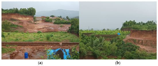
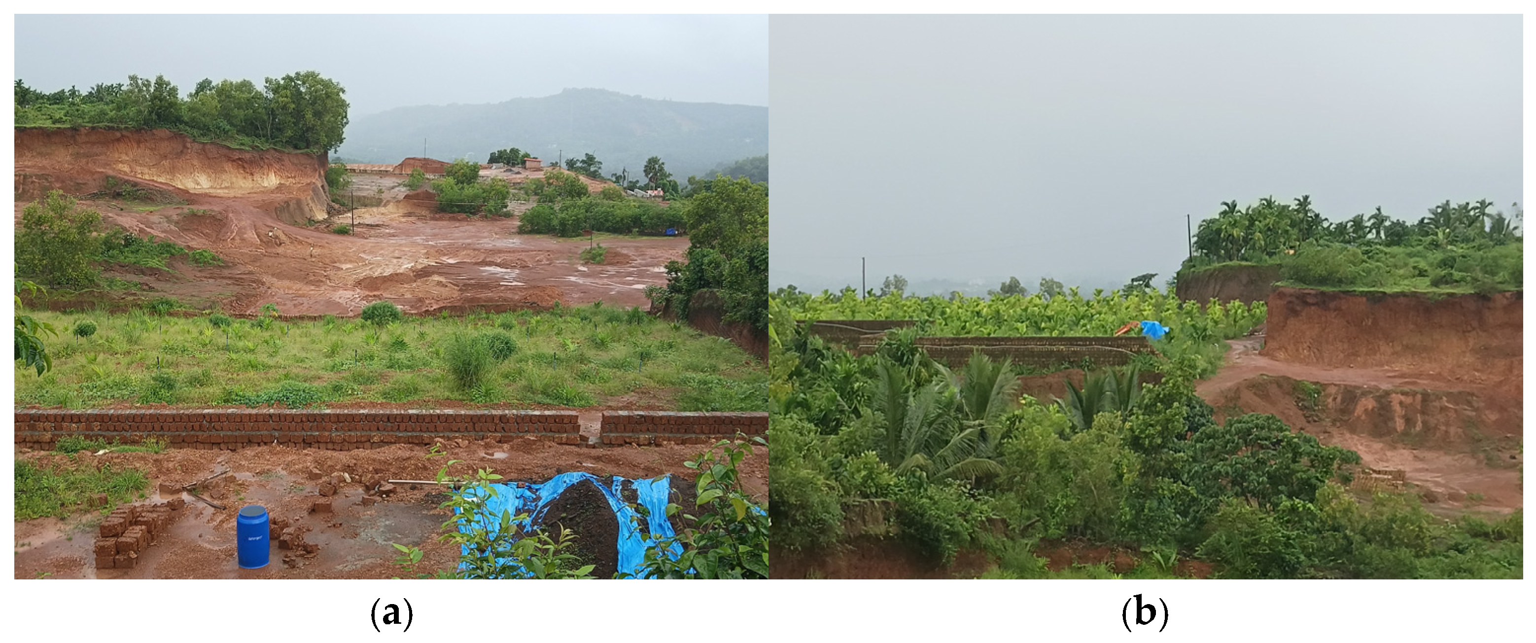
Field observations at two nearby former mining sites (Figure 12) illustrate how such areas are being reclaimed. The first location is adjacent to ongoing construction activity and recently planted arecanut saplings, with no laterite remaining available for extraction. The second location, where extraction had ended earlier, has since been fully reclaimed into an established, mature arecanut plantation.
Figure 12.
Field photographs of two nearby former laterite mining sites in Bantwal Taluk, illustrating variable reclamation outcomes: (a) recently exhausted site with construction activity and newly planted arecanut saplings; (b) nearby site, extraction ended earlier, established mature arecanut plantation. Locations confirmed through direct field observation by the author.
These photographs show what is occurring at just two locations among the several square kilometers of mined land across the taluk, and cannot be assumed to represent the full range of possible outcomes. They do, however, indicate that mining sites in this taluk are reclaimed toward variable end uses rather than a single consistent outcome.
4.4. Methodological Limitations and Future Research
A number of methodological constraints should be considered when interpreting these results. Single-date Landsat images reduce the amount of phenologic variability observed; however, they will not capture intra-annual mining activity or short-term reclamation. Seasonal composites (such as median or cloud-free composites covering multiple months) have not been utilized in this study, since compositing through the monsoon-to-dry-season transition may introduce the same Barren Land–Built-up spectral confusion mentioned earlier, along with the annual changes in vegetation phenology. Thus, careful selection of a single, low-cloud, dry-season scene per epoch is viewed as the most consistent basis for a two-point decadal comparison. Given the time-varying nature of the mining footprint, it is possible that some activity could begin and end entirely within the ten-year window between the two scenes, and such activity would not be captured by either image. Additionally, the 30-m spatial resolution of the Landsat data sets an absolute minimum size for a feature to be reliably detected using these images. Since this research utilized TOA reflectance instead of surface reflectance, it should be noted that Zhu et al. [35] found that surface reflectance typically outperforms TOA reflectance for change detection applications. While the use of TOA data in this case was partially mitigated by the dry-season image collection period and low amounts of cloud cover, there are still potential limitations associated with its application.
The classification uncertainty of this research is described by confusion matrices (Figure 7 and Figure 9), which show that uncertainty is concentrated primarily in the Barren Land and Built-up classes, as they have the lowest per-class F1-scores and the highest mutual spectral confusion (Section 4.1). Future research could include pixel-based classification probabilities to provide confidence maps.
The classification of features into three categories based upon their presence in the 2015 versus 2025 mining reference layers was achieved by comparing the two reference layers directly. Features appearing in both layers were classified as “persistent,” only in 2015 as “reclaimed,” and only in 2025 as “new.” In this way, this process avoided the possibility of epoch-to-epoch classifier noise, yet provided information about the accuracy of the reference data rather than the ability of the classifier to accurately identify changes over time.
While manual digitization provides completely noise-free data, it is extremely labor-intensive and therefore does not lend itself well to being scaled up to larger geographic areas. Automated alternatives do exist; for example, deep learning classifiers can be trained to automatically identify mining boundaries at finer resolution than 30 m using Sentinel-2 imagery. In fact, Mehta et al. [2] successfully used such a technique to automatically classify hundreds of mining sites throughout India using higher-resolution Sentinel-2 imagery. Similarly, Saputra et al. [36] demonstrated the effectiveness of multi-modal deep learning for segmenting individual mining footprints at the pixel level from multispectral imagery. Combining an automated detection capability with the manually validated approach employed in this research for ground-truthing would provide a viable means for expanding this methodology to larger geographic areas and provide a more complete view of the extent and distribution of mining activity within a particular region.
Field observation also suggests that laterite mining is comparatively more extensive in neighboring taluks within Dakshina Kannada District, making them natural candidates for extending this methodology to a more intensive mining context and a fuller district-wide picture.
4.5. Management Implications
With reference to the spatial turnover noted above, the almost equal number of newly created (71) and reclaimed (68) mining sites, along with the persistent footprint of just 0.296 km2 (less than 9% of the union footprint), highlights the spatial turnover rate of the active sites during the ten-year period. Such spatial turnover of the sites also has implications for the monitoring of mining activities within the taluk: any inventory of existing sites will soon become obsolete due to the tendency of mining activity to change locations frequently. The 68 reclaimed sites also have implications for reclamation monitoring: according to field observations (see Figure 12), the reclamation status of neighboring sites can vary, meaning that the reclamation process does not end with the closure of a site.
5. Conclusions
This research shows that a transferable framework, combining XGBoost-based land cover classification with GIS-based mining footprint extraction, utilizing free Landsat 8 and Landsat 9 images along with standardized pre-processing and classification techniques, is capable of reliable, decadal-scale monitoring of land cover change as well as laterite mining activities in a coastal region of India. Notably, the classifier demonstrated strong performance in both time frames, with weighted F1 scores of 0.944 (2015) and 0.904 (2025); the modest decline reflects increased spectral confusion between Barren Land and Built-up classes rather than a fundamental methodological weakness, though it underscores that classification outputs for these two classes should be interpreted with appropriate caution in operational decision-making contexts. Over the study decade, a substantial amount of land-cover change occurred throughout Bantwal Taluk, with Barren Land primarily converting to Agricultural and Built-Up uses, alongside a marked increase in surface water extent linked to regional dam construction; these changes are, in turn, likely attributable to a combination of natural recovery from previous disturbances, local economic conditions, and regional infrastructure development. Against this broader backdrop, the analysis of mining footprints identified 71 newly mined areas and 68 reclaimed mining areas during the same time frame, with a total union footprint of approximately 3.315 km2, roughly 1.8 times the mining extent detectable in any single epoch. This indicates, ultimately, that the mining landscape is not static or linear, but rather dynamic. These findings should be interpreted within the study’s methodological scope: reliance on two single-date images and Top-of-Atmosphere reflectance, rather than a continuous time series or surface reflectance, means that the results capture decadal snapshots rather than continuous monitoring, a trade-off that favored data accessibility and processing simplicity over finer temporal resolution.
Overall, this study provides a spatial-temporal view of laterite mining activity down to the individual feature level, by combining validated land-cover classification with a persistent, new, and reclaimed framework, and presents a low-cost, transferable strategy for environmental monitoring. For district mining authorities, this suggests prioritizing periodic, taluk-wide footprint reassessment over static site monitoring, given the high turnover between new and reclaimed sites, and extending reclamation verification beyond initial site closure. This approach could similarly support land degradation tracking and sustainable resource management in other coastal, laterite mining regions.
Author Contributions
J.B.K.: Conceptualization, Methodology, Software, Writing—Original Draft. O.P.K.: Data Curation, Validation, Supervision. S.V.: Supervision, Software, Writing—Review and Editing. A.S.A.: Investigation, Data Curation, Validation. R.R.: Investigation, Formal Analysis, Visualization. B.B.K.: Supervision, Formal Analysis, Visualization. B.G.: Software, Writing—Original Draft. Y.-J.C.: Methodology, Validation, Writing—Review and Editing. All authors have read and agreed to the published version of the manuscript.
Funding
This research received no external funding.
Institutional Review Board Statement
Not applicable.
Informed Consent Statement
Not applicable.
Data Availability Statement
The data presented in this study are contained within the article.
Conflicts of Interest
The authors declare no conflicts of interest.
Abbreviations
The following abbreviations are used in this manuscript:
| NDVI | Normalized Difference Vegetation Index |
| NDBI | Normalized Difference Built-up Index |
| NDWI | Normalized Difference Water Index |
| XGBoost | Extreme Gradient Boosting |
| NRSC | National Remote Sensing Centre |
| TOA | Top-of-Atmosphere |
| MMU | Minimum Mapping Unit |
| IoU | Intersection-over-Union |
| LULC | Land Use/Land Cover |
| RF | Random Forest |
| SVM | Support Vector Machine |
References
- Mutimba, K.; Watanabe, T.; Chand, M.B. Land Use Land Cover (LULC) Change Dynamics Associated with Mining Activities in Kitwe District and Adequacy of the Legal Framework on Mine Closure in Zambia. Earth 2024, 5, 110–132. [Google Scholar] [CrossRef] [Scilit]
- Mehta, S.A.; Ashish; Solanki, M.; Seth, A. A Characterization of Land-use Changes in the Proximity of Mining Sites in India. ACM J. Comput. Sustain. Soc. 2024, 2, 10. [Google Scholar] [CrossRef] [Scilit]
- Vandana, M.; John, S.; Sunny, S.; Maya, K.; Padmalal, D. Environmental impact assessment of laterite quarrying from Netravati- Gurpur river basin, South West Coast of India. Environ. Dev. Sustain. 2024, 26, 909–930. [Google Scholar]
- Kumar, G.S.; Saini, P.K.; Deoliya, R.; Mishra, A.K.; Negi, S.K. Characterization of laterite soil and its use in construction applications: A review. Resour. Conserv. Recycl. Adv. 2022, 16, 200120. [Google Scholar] [CrossRef] [Scilit]
- Vadrevu, K.P.; Ohara, T. Focus on land use cover changes and environmental impacts in South/Southeast Asia. Environ. Res. Lett. 2020, 15, 100201. [Google Scholar] [CrossRef] [Scilit]
- Bhagyashree; Udayashankar, H.N.; Sarvade, P.; Kavyashree. Correlation of Mineralogical and Geotechnical Properties of Laterite Soils of Coastal Karnataka, India. Civ. Eng. Archit. 2023, 11, 3334–3346. [Google Scholar] [CrossRef] [Scilit]
- Sowmya; Athishri, A.N.; Raghudas, J.D.; Abhishek, R.; Chalannavar, R.K. Urban dispersion-driven land use change detection using GIS-based buffer gradient and Shannon’s entropy analysis in Dakshina Kannada District, India. Environ. Monit. Assess. 2026, 198, 362. [Google Scholar] [CrossRef] [Scilit] [PubMed]
- Kamga, M.A.; Nguemhe Fils, S.C.; Ayodele, M.O.; Olatubara, C.O.; Nzali, S.; Adenikinju, A.; Khalifa, M. Evaluation of land use/land cover changes due to gold mining activities from 1987 to 2017 using Landsat imagery, East Cameroon. GeoJournal 2020, 85, 1097–1114. [Google Scholar] [CrossRef] [Scilit]
- Jafarzadeh, H.; Mahdianpari, M.; Gill, E.; Mohammadimanesh, F.; Homayouni, S. Bagging and Boosting Ensemble Classifiers for Classification of Multispectral, Hyperspectral and PolSAR Data: A Comparative Evaluation. Remote Sens. 2021, 13, 4405. [Google Scholar] [CrossRef] [Scilit]
- Uthappa, A.R.; Das, B.; Chavan, S.B.; Raizada, A.; Desai, S.; Paramesha, V.; Kumar, P.; Jha, P.K.; Vara Prasad, P.V. Comparison of machine learning models for mapping Arecanut based agroforestry system in Goa by enhancing precision and efficiency. Sci. Rep. 2025, 15, 44280. [Google Scholar] [CrossRef] [Scilit] [PubMed]
- Khan, S.; Bhardwaj, A.; Sakthivel, M. Accuracy Assessment of Land Use Land Cover Classification Using Machine Learning Classifiers in Google Earth Engine; A Case Study of Jammu District. Int. Arch. Photogramm. Remote Sens. Spat. Inf. Sci. 2024, XLVIII-4-2024, 263–268. [Google Scholar] [CrossRef] [Scilit]
- Shree, N.G.; Meiaraj, C. Land use and land cover change detection by machine learning classifiers (SVM and RF) using satellite remote sensing observations for Cuddalore Taluk, Tamil Nadu, India. J. Earth Syst. Sci. 2025, 134, 22. [Google Scholar] [CrossRef] [Scilit]
- Rawat, K.S.; Kumar, S.; Garg, N. Statistical Comparison of Simple and Machine Learning Based Land Use and Land Cover Classification Algorithms: A Case Study of Chennai District. J. Water Manag. Model. 2024, 32, H524. [Google Scholar] [CrossRef] [Scilit]
- Buthelezi, M.N.M.; Lottering, R.T.; Peerbhay, K.Y.; Mutanga, O. Predicting land use and land cover change dynamics in the eThekwini Municipality: A machine learning approach with Landsat imagery. J. Spat. Sci. 2024, 69, 1241–1263. [Google Scholar] [CrossRef] [Scilit]
- Gurjar, Y.; Wen, R.; Farahbakhsh, E.; Chandra, R. Landcover Classification and Change Detection Using Remote Sensing and Machine Learning: A Case Study of Western Fiji. Adv. Space Res. 2026, 77, 8521–8537. [Google Scholar] [CrossRef] [Scilit]
- Ren, H.; Zhao, Y.; He, T. Remote Sensing in Mining-Related Eco-Environmental Monitoring and Assessment. Remote Sens. 2026, 18, 103. [Google Scholar] [CrossRef] [Scilit]
- Vandana, M.; John, S.E.; Maya, K.; Padmalal, D. Environmental impact of quarrying of building stones and laterite blocks: A comparative study of two river basins in Southern Western Ghats, India. Environ. Earth Sci. 2020, 79, 366. [Google Scholar] [CrossRef] [Scilit]
- Vandana, M.; John, S.E.; Maya, K.; Sunny, S.; Padmalal, D. Environmental impact assessment (EIA) of hard rock quarrying in a tropical river basin: Study from the SW India. Environ. Monit. Assess. 2020, 192, 580. [Google Scholar] [CrossRef] [Scilit] [PubMed]
- Cuypers, S.; Nascetti, A.; Vergauwen, M. Land Use and Land Cover Mapping with VHR and Multi-Temporal Sentinel-2 Imagery. Remote Sens. 2023, 15, 2501. [Google Scholar] [CrossRef] [Scilit]
- Radeloff, V.C.; Roy, D.P.; Wulder, M.A.; Anderson, M.; Cooke, B.; Crawford, C.J.; Friedl, M.; Gao, F.; Gorelick, N.; Hansen, M.; et al. Need and vision for global medium-resolution Landsat and Sentinel-2 data products. Remote Sens. Environ. 2024, 300, 113918. [Google Scholar] [CrossRef] [Scilit]
- Voskanian, N.; Thome, K.J.; Wenny, B.N.; Tahersima, M.H.; Yarahmadi, M. Combining RadCalNet Sites for Radiometric Cross Calibration of Landsat 9 and Landsat 8 Operational Land Imagers (OLIs). Remote Sens. 2023, 15, 5752. [Google Scholar] [CrossRef] [Scilit]
- Dampuru, V.N.S.P.K.; Sharma, K.K.; Rajender, P. Strengthening safety and regulatory framework in stone quarries (Minor Mineral) for Sustainable Infrastructure in India. Int. J. Sci. Res. Arch. 2025, 15, 1200–1204. [Google Scholar] [CrossRef] [Scilit]
- Verma, V. Exploring Key XGBoost Hyperparameters: A Study on Optimal Search Spaces and Practical Recommendations for Regression and Classification. Int. J. All. Res. Educ. Sci. Methods 2024, 12, 3259–3266. [Google Scholar] [CrossRef] [Scilit]
- Velarde, G.; Weichert, M.; Deshmunkh, A.; Deshmane, S.; Sudhir, A.; Sharma, K.; Joshi, V. Tree boosting methods for balanced and imbalanced classification and their robustness over time in risk assessment. Intell. Syst. Appl. 2024, 22, 200354. [Google Scholar] [CrossRef] [Scilit]
- Pande, C.B.; Srivastava, A.; Moharir, K.N.; Radwan, N.; Sidek, L.M.; Alshehri, F.; Pal, S.C.; Tolche, A.D.; Zhran, M. Character- izing land use/land cover change dynamics by an enhanced random forest machine learning model: A Google Earth Engine implementation. Environ. Sci. Eur. 2024, 36, 84. [Google Scholar] [CrossRef] [Scilit]
- Almohamad, H.; Alshwesh, I.O. Evaluation of Index-Based Methods for Impervious Surface Mapping from Landsat-8 to Cities in Dry Climates; A Case Study of Buraydah City, KSA. Sustainability 2023, 15, 9704. [Google Scholar] [CrossRef] [Scilit]
- Kebede, T.A.; Hailu, B.T.; Suryabhagavan, K.V. Evaluation of spectral built-up indices for impervious surface extraction using Sentinel-2A MSI imageries: A case of Addis Ababa city, Ethiopia. Environ. Chall. 2022, 8, 100568. [Google Scholar] [CrossRef] [Scilit]
- Nandam, V.; Patel, P.L. A novel hybrid approach using SVM and spectral indices for enhanced land use land cover mapping of coastal urban plains. Geocarto Int. 2022, 37, 4714–4736. [Google Scholar] [CrossRef] [Scilit]
- Maloney, M.C.; Becker, S.J.; Griffin, A.W.H.; Lyon, S.L.; Lasko, K. Automated Built-Up Infrastructure Land Cover Extraction Using Index Ensembles with Machine Learning, Automated Training Data, and Red Band Texture Layers. Remote Sens. 2024, 16, 868. [Google Scholar] [CrossRef] [Scilit]
- Quash, Y.; Kross, A.; Jaeger, J.A.G. Assessing the impact of gold mining on forest cover in the Surinamese Amazon from 1997 to 2019: A semi-automated satellite-based approach. Ecol. Inform. 2024, 80, 102442. [Google Scholar] [CrossRef] [Scilit]
- Vivek, M.C.; Sahana, S.; Patil, K.K.R. Price Behaviour of Arecanut in the State of Karnataka (India) Under e-tendering Regime. Indian J. Ext. Educ. 2021, 57, 93–98. [Google Scholar]
- Government of Karnataka; Directorate of Economics and Statistics. Karnataka Economic Survey 2025–26; Government of Karnataka: Bengaluru, India, 2026.
- Government of Karnataka; Minor Irrigation and Ground Water Development Department. Annual Report 2022–23. Available online: https://minorirrigation.karnataka.gov.in/storage/pdf-files/ANNUAL%20REPORT/2022-23.pdf (accessed on 22 August 2026).
- Madhav, R. Environmental Governance of Artisanal and Small-Scale Mining in India. Asian Aff. 2020, 51, 895–912. [Google Scholar] [CrossRef] [Scilit]
- Zhu, Z.; Zhang, J.; Yang, Z.; Aljaddani, A.H.; Cohen, W.B.; Qiu, S.; Zhou, C. Continuous monitoring of land disturbance based on Landsat time series. Remote Sens. Environ. 2020, 238, 111116. [Google Scholar] [CrossRef] [Scilit]
- Saputra, M.R.U.; Bhaswara, I.D.; Nasution, B.I.; Ern, M.A.L.; Husna, N.L.R.; Witra, T.; Feliren, V.; Owen, J.R.; Kemp, D.; Lechner, A.M. Multi-modal deep learning approaches to semantic segmentation of mining footprints with multispectral satellite imagery. Remote Sens. Environ. 2025, 318, 114584. [Google Scholar] [CrossRef] [Scilit]

Disclaimer/Publisher’s Note: The statements, opinions and data contained in all publications are solely those of the individual author(s) and contributor(s) and not of MDPI and/or the editor(s). MDPI and/or the editor(s) disclaim responsibility for any injury to people or property resulting from any ideas, methods, instructions or products referred to in the content. |
© 2026 by the authors. Licensee MDPI, Basel, Switzerland. This article is an open access article distributed under the terms and conditions of the Creative Commons Attribution (CC BY) license.