Amazon Deforestation and Land Use Emissions: Annual Relationships with Hydroclimate and Agricultural Value Added

Abstract

Forest loss in the Amazon links land conversion to carbon emissions and may alter the climatic conditions that support agriculture. This study examines how these relationships unfold within and across years using regional observations for 1990–2023. Exploratory analyses and a Bayesian vector autoregression relate deforestation, temperature, precipitation, gross land use emissions, and agricultural value added, accounting for Pacific and Atlantic climate variability and a linear trend. Deforestation and emissions remain grouped after removing trends, whereas the broader climatic and agricultural groupings change. Changes in deforestation and emissions are positively associated within the same year: a one standard deviation unexpected increase in annual deforestation change corresponds to an estimated emissions change response of 115.87 million tCO₂e (95% credible interval: 56.33–192.20 million). Subsequent responses are too uncertain to establish how long this association persists. Temperature, precipitation, and agricultural responses also remain imprecisely estimated. The principal contribution is an integrated assessment distinguishing detectable annual forest loss–inventory co-movement from unresolved later hydroclimatic and agricultural responses. Related land change inputs in the emissions inventory limit the independence of the carbon finding. These results support joint monitoring of forest loss and gross emissions, complemented by spatial and seasonal indicators of climatic regulation and agricultural vulnerability.

1. Introduction

The Amazon forest is a central component of the South American climate system. Through evapotranspiration and atmospheric moisture recycling, it influences regional precipitation, surface energy balances, atmospheric circulation, and water availability within and beyond the basin [1,2,3]. Forest loss modifies evapotranspiration, surface roughness, albedo, and sensible and latent heat fluxes, potentially affecting both local climatic conditions and downwind regions. These interactions are spatially heterogeneous and vary according to season, land use configuration, forest loss intensity, and the geographical scale at which climatic responses are measured [4,5,6].

The consequences of deforestation are not restricted to hydroclimatic processes. Clear-cutting, degradation, fire, and associated land cover transitions contribute to greenhouse gas emissions from land use, land use change, and forestry (LULUCF) and can alter the regional carbon balance [7,8]. Agricultural outcomes are similarly mediated by several mechanisms, including rainfall, productivity, commodity prices, rural credit, technology, environmental enforcement, and the availability of previously cleared land. Consequently, agricultural expansion and aggregate output do not necessarily move proportionally with annual forest loss [9,10,11]. Understanding how these indicators vary together is relevant to assessing land conversion alongside the climatic conditions on which agricultural activity depends.

The identification of deforestation-related dynamics is further complicated by large-scale climate variability. The El Niño–Southern Oscillation (ENSO) is a major source of interannual rainfall and temperature anomalies in Amazonia and closely associated with drought intensity, fire occurrence, and carbon emissions [5,7,12]. Climatic variation associated with ENSO may therefore coincide with or obscure the hydroclimatic responses associated with land use change. Tropical Atlantic conditions also influence Amazonian drought and rainfall variability [12]. The annual comparison therefore includes both the Oceanic Niño Index (ONI) and a Tropical North Atlantic index (TNA) while recognizing that these controls cannot represent all climatic and socioeconomic influences.

Previous studies have documented hydroclimatic responses [4,5,6,12], carbon dynamics [7,8], and relationships between agriculture, land use, and deforestation [4,9,10,11]. More recent studies have connected some of these dimensions. Franco et al. examine the interaction of deforestation and climate change in the transformation of the Amazon rainforest [13], whereas Attílio examines Amazon deforestation and CO₂ emissions within a global vector autoregressive framework [14]. Other multivariate studies have focused on the economic drivers of deforestation [15] or transitions among land use categories [16]. Together, these studies address forest loss through different measurements, geographical scales, and environmental or economic outcomes.

The central question of this study is how annual changes in Amazon deforestation relate to emissions, hydroclimate, and agricultural activity and how these relationships unfold over time after accounting for oceanic climate variability. To address this question, the study examines regional temperature, precipitation, gross LULUCF emissions, and agricultural value added in relation to annual changes in deforestation in the Brazilian Legal Amazon. The objectives are to identify patterns of co-movement among these indicators; compare the timing, persistence, and uncertainty of responses associated with deforestation innovations; and quantify the share of each outcome’s forecast error variance associated with those innovations, conditional on ENSO and tropical Atlantic variability. The empirical contribution is an integrated assessment of the annual relationships linking forest loss, emissions, hydroclimatic conditions, and agricultural activity, distinguishing same-year associations from responses in subsequent years.

The empirical strategy combines exploratory multivariate analysis with Bayesian dynamic modeling using annual observations for 1990–2023. Hierarchical cluster analysis (HCA) and principal component analysis (PCA) describe similarities among the series and their main axes of co-movement, both in levels and after transformation. A Bayesian vector autoregression with external regressors (BVARX), estimated with a Litterman–Minnesota coefficient prior [17], models the dynamic relationships conditional on ONI, TNA, and a linear trend, with sensitivity evaluated across alternative prior and lag specifications [18,19]. Generalized impulse response functions (GIRFs) trace the responses to innovations in annual deforestation changes, while normalized generalized forecast error variance decompositions (GFEVDs) summarize their associated shares of forecast uncertainty within the model [20]. Conditional Granger tests provide complementary evidence on predictive directionality. The resulting comparisons describe annual associations; they do not identify an externally imposed forest clearing intervention.

2. Materials and Methods

2.1. Data Coverage and Annual Definitions

The dataset contains 34 complete annual observations for 1990–2023, the common period available for all indicators. The endogenous variables are deforestation (PRODES), 2 m air temperature (TEMP), precipitation (PREC), gross land use, land use change and forestry emissions (CO2E), and agricultural value added (AGRO); ONI and TNA are external regressors. No missing annual value was imputed. Table 1 defines their units, geographic coverage, and annual windows. Source extraction and verification details are provided in Supplementary Material S1.

Table 1. Definitions and temporal coverage of the analytical variables.

Variable and Unit	Geographic Scope and Source	Annual Definition
PRODES (km2)	Official Legal Amazon monitoring domain; INPE [21]	August(t − 1)–July(t); annual clear-cut deforestation rate
TEMP (°C)	IBGE 2024 Legal Amazon polygon; ERA5-Land 0.1° [22,23,24]	August–July; day-weighted mean of monthly means
PREC (mm)	IBGE 2024 Legal Amazon polygon; CHIRPS v2.0, 0.05° [25]	August–July; sum of monthly precipitation totals
CO2E (tCO2e)	SEEG 13; gross LULUCF, GWP100 AR6; listed Legal Amazon municipalities [26]	Calendar year; annual inventory total
AGRO (million 2010 BRL)	Ipeadata; sum of nine whole states, including all of Maranhão [27]	Calendar year; agricultural gross value added at basic prices
ONI (°C)	NOAA CPC, ERSSTv5 Niño-3.4 index [28]	August–July mean of 12 overlapping seasons assigned to their central month
TNA (°C)	NOAA PSL HadISST1.1, 1991–2020 anomaly baseline [29]	August–July mean of 12 monthly anomalies

All main-series observations cover 1990–2023. The nine states are Acre, Amapá, Amazonas, Maranhão, Mato Grosso, Pará, Rondônia, Roraima, and Tocantins. The spatial supports of the indicators are related but not identical. GWP100 AR6 denotes 100-year global warming potentials from the IPCC Sixth Assessment Report.

Climate aggregates use grid cells whose centers fall within the IBGE 2024 Legal Amazon polygon, with cosine latitude weights renormalized over valid cells. ERA5-Land temperatures were converted to degrees Celsius and combined into annual means weighted by the number of days per month. Annual CHIRPS precipitation sums 12 monthly regional totals. The August–July climate and ocean index windows align with the official PRODES year; CO2E and AGRO retain calendar-year totals. ONI three-month seasons were assigned to their central month before annual averaging. Alternative July–June and calendar-year windows were evaluated for TEMP, PREC, ONI, and TNA.

SEEG 13 emissions were filtered for gross LULUCF emissions under GWP100 AR6, excluding removals and other sectors, and aggregated using the IBGE 2024 Legal Amazon municipal list. The main series includes the full totals of the 181 listed Maranhão municipalities, including 21 partially within the region. A sensitivity analysis weights these partial municipalities by their territorial shares. The SEEG methodology combines the MapBiomas collection of 10 land cover transitions and deforestation/regeneration information with national inventory carbon stocks and IPCC accounting methods [26].

AGRO sums the nine whole-state Ipeadata series in million constant 2010 BRL and covers agriculture, livestock, forestry, fishing, and aquaculture. Its source metadata identify different Regional Accounts systems, including a comparability break in 2002. Sensitivity analyses exclude AGRO or Maranhão, use agricultural log changes, and include pulse and level-shift controls for 2002. The indicators thus differ in geographic coverage and annual windows, as specified in Table 1.

2.2. Exploratory Structure and Transformation of the Series

HCA groups standardized annual trajectories using Euclidean distances and Ward.D2 linkage [30], with the number of groups selected by average silhouette width. PCA summarizes the correlation matrix of the same seven variables [31]; component retention uses Gaussian and temporal circular-shift parallel analysis [32]. Alternative distance/linkage combinations and a common-window comparison assess sensitivity. Simulation settings and agreement measures are given in S1.

HCA and PCA were applied to levels for 1990–2023 and transformed series for 1991–2023. The latter use first differences of PRODES, CO2E, and AGRO and residuals from intercept and trend regressions for TEMP, PREC, ONI, and TNA. These comparisons assess how trends influence the multivariate grouping.

Stationarity was assessed using Augmented Dickey–Fuller (ADF), Phillips–Perron (PP), and Kwiatkowski–Phillips–Schmidt–Shin (KPSS) tests [33,34,35]. Level tests include an intercept and trend; first-difference tests include an intercept. Zivot–Andrews tests allow one endogenous intercept-and-trend break [36]. Lag selection, bandwidths, and critical values are documented in S1.

The modeling vector uses first differences of PRODES, CO2E, and AGRO and retains TEMP and PREC in levels with an explicit linear trend; ONI and TNA also remain in levels. Temperature differencing and alternative agricultural transformations were evaluated as sensitivities. Differencing yields 33 observations for 1991–2023. Model comparisons reserve 1991–1993 as initial lag history and use the same 30 response observations for 1994–2023.

2.3. Bayesian Model and Prior Grid

Let y_t = (ΔPRODES_t, TEMP_t, PREC_t, ΔCO2E_t, ΔAGRO_t)′ and let z_t contain a centered linear trend, ONI, and TNA. The reduced form model is [37]

$$y_t=c+{\sum }_{l=1}^p{A}_l{y}_{t-l}+\Gamma z_t+u_t,u_t\sim N_5(0,\Sigma )$$

(1)

Candidate lag orders are p = 0, 1, 2, and 3. Each equation has four non-lag regressors and 5p lag coefficients. Scaling and a pilot innovation covariance, estimated from own-AR(1) regressions with the same controls, were calculated within each training sample.

The coefficient vector β = vec(B) has a zero-mean normal prior with diagonal covariance V₀. In standardized units, own-lag prior standard deviations are λ₁ divided by l to the power λ₃ and cross-lag standard deviations additionally multiply by λ₂; intercept and control priors are diffuse. The grid uses λ₁ ∈ {0.1, 1, 5, 10}, λ₂ = 0.99, and λ₃ ∈ {1, 2}, giving 21 distinct specifications after removing duplicate one-lag priors. Conditional on Σ, the joint Gaussian posterior has precision and mean

$$Q={V_0}^{-1}+{\Sigma }^{-1}\otimes \left(X^{\prime }X\right),$$

$$E\left(\beta \right|Y,\Sigma )=Q^{-1}\mathrm{v}\mathrm{e}\mathrm{c}(X^{\prime }Y{\Sigma }^{-1})$$

(2)

The posterior covariance is Q⁻¹. The p = 0 model is a multivariate regression on the controls and provides a predictive benchmark; positive-lag models allow responses to propagate across years.

2.4. Forecast Comparison and Residual Screening

Conditional one-step forecasts were evaluated over 2011–2023 using expanding windows and rolling windows of 20 observations. Each forecast conditions on realized contemporaneous ONI and TNA. The comparison score averages variable-specific RMSEs, normalized by evaluation period standard deviations, across both window schemes. Because these years also inform prior selection, this is a conditional evaluation used for model comparison.

AIC and BIC provide auxiliary fit–complexity summaries using nominal counts and an effective coefficient count tr(Q⁻¹L), where L = Σ⁻¹ ⊗ (X′X), plus 15 covariance parameters. Dynamic stability requires the maximum companion root modulus of the coefficient posterior mean to be below one.

Residual serial dependence was evaluated using recursive Gaussian parametric bootstraps with complete model refitting. Six global diagnostics assess equation-level and multivariate dependence; the strict screen additionally requires nonrejection of each equation’s Ljung–Box statistic at horizons four and six. The primary dynamic model minimizes the combined forecast RMSE among stable positive-lag candidates passing this screen at 5%. The best candidate under the global screen and the p = 0 benchmark are reported separately. Monte Carlo intervals describe uncertainty around screening probabilities; these decision rules have no established joint familywise error rate. Full definitions and simulation settings appear in S1.

2.5. Posterior Uncertainty and Dynamic Summaries

Lag–prior sensitivity uses Gaussian coefficient draws conditional on the pilot covariance. Primary uncertainty estimates use independent priors β ∼ N(0, V₀) and Σ ∼ IW(m + 2, Σ_pilot), where m = 5 and the covariance prior mean equals Σ_pilot. Gibbs sampling alternates the joint normal coefficient conditional and the inverse-Wishart covariance conditional. Effective sample sizes and split-chain R-hat assess sampling performance; iteration counts and update equations are provided in S1.

Main summaries condition on dynamic stability, with unrestricted summaries supplied as sensitivity results. Intervals incorporate coefficient and innovation covariance uncertainty while remaining conditional on model selection, empirical scaling, and prior calibration.

A generalized impulse response to a positive one standard deviation innovation in ΔPRODES is calculated for each posterior draw as

$$g_j(h)={\displaystyle \frac{{\Phi }_h\Sigma e_j}{\sqrt{{\sigma }_{jj}}}},{\Phi }_0=I_m$$

(3)

Here, e_j selects the deforestation equation and Φ_h is the moving-average response matrix. Impact is h = 0; h = 1 is one year later. Covariance uncertainty is propagated into the impact response. Responses are expressed in native units, with cumulative summaries also supplied for first-differenced variables. For PRODES, these cumulative responses describe changes in the annual deforestation rate level.

Generalized forecast error variance shares are computed at H = 1, 5, 10, and 20. For response i and innovation j, the unnormalized draw-specific share is

$${\theta }_{ij}(H)={\displaystyle \frac{{{\sigma }_{jj}}^{-1}{\sum }_{h=0}^{H-1}{({e_i}^{\prime }{\Phi }_h\Sigma e_j)}^2}{{\sum }_{h=0}^{H-1}{e_i}^{\prime }{\Phi }_h\Sigma {{\Phi }_h}^{\prime }{e}_i}}$$

(4)

Shares are normalized across innovations within each draw before posterior medians and 95% pointwise credible intervals are calculated. H = 1 includes impact only; H = 20 provides a long-horizon sensitivity summary. Generalized responses accommodate contemporaneously correlated innovations without recursive ordering restrictions [20]. They describe conditional associations, and normalized variance shares allocate forecast uncertainty within the model.

2.6. Predictability, Stability, and Specification Sensitivity

Conditional Granger tests use OLS VARX equations with all endogenous variables and controls at lags one to three. Holm and Benjamini–Hochberg adjustments apply to the family of 60 directional tests [38,39]. Parameter stability is examined in own-ARX(1) equations using a 2002 break and a maximum-F search over 2005–2013 [40] calibrated by independent and block wild bootstraps with Holm adjustment. These tests concern conditional predictability and own-equation stability.

Nineteen specifications assess smaller systems, control removal, stronger shrinkage, alternative annual windows and geographic aggregation, agricultural transformations and break controls, temperature differencing, subsamples, and an extension through 2024 without AGRO. These comparisons use fixed-covariance coefficient draws. Statistical estimation and posterior summaries were produced in R (version 4.6.1); manuscript figures were rendered from the saved R outputs. Supplementary Material S2 supplies the data, custom BVARX implementation, analysis code, and complete numerical results.

3. Results

3.1. Annual Environmental and Agricultural Patterns

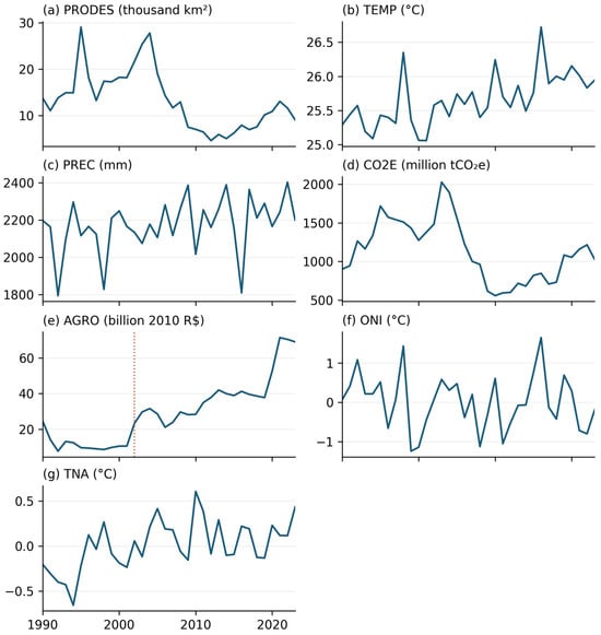
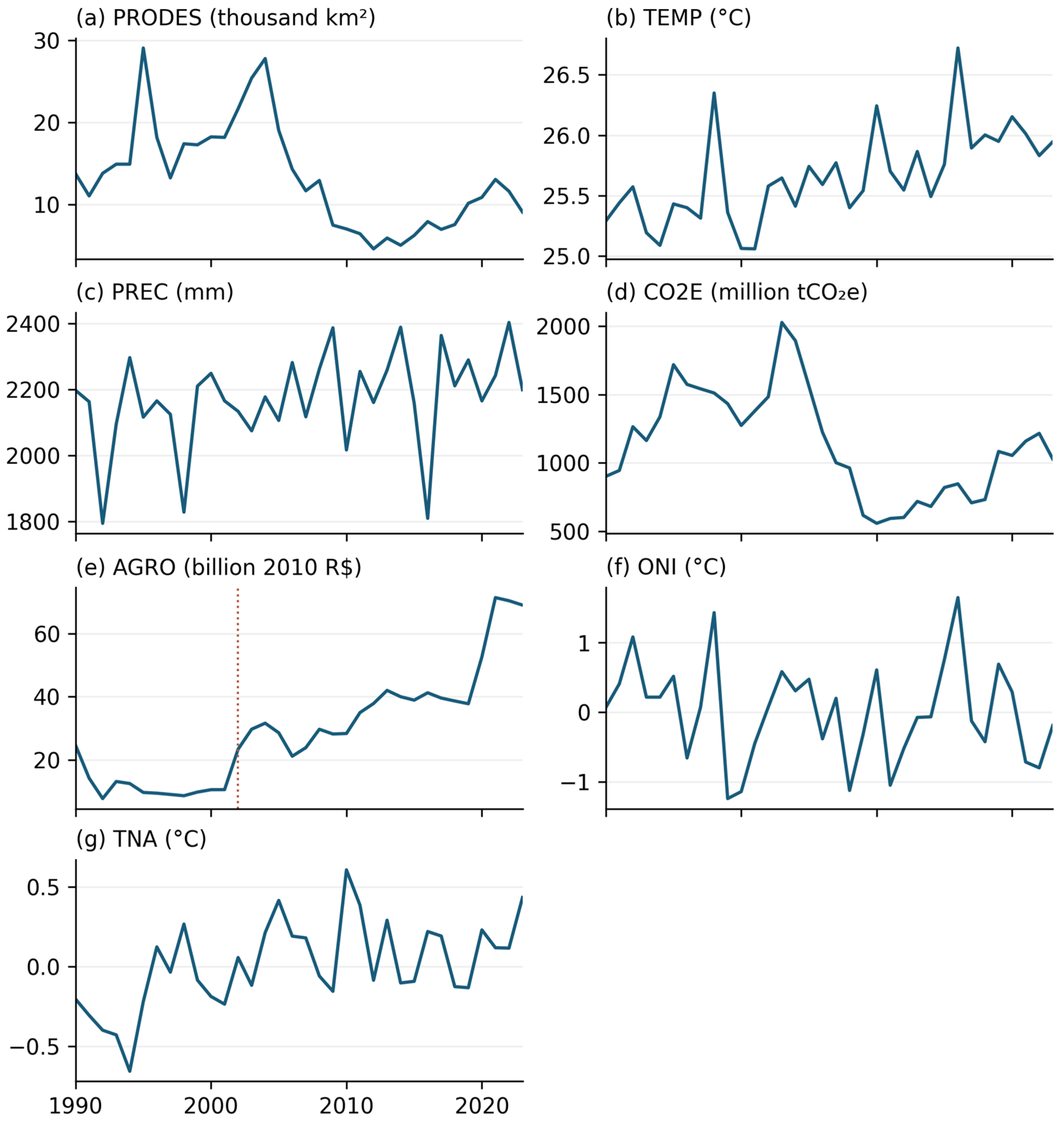
Annual deforestation varies substantially over 1990–2023, averaging 13,297 km² and ranging from 4571 to 29,059 km². Gross LULUCF emissions average approximately 1.136 billion tCO₂e per year, with a range of 557.53–2028.14 million tCO₂e. Regional mean temperature ranges from 25.06 to 26.72 °C and annual precipitation from 1794 to 2402 mm (Table 2). Figure 1 places these environmental trajectories alongside agricultural activity and oceanic climate variability.

Table 2. Descriptive statistics of the level series, 1990–2023 (n = 34).

Variable	Unit	Mean	SD	Minimum	Maximum
PRODES	km2	13,297.44	6362.51	4571.00	29,059.00
TEMP	°C	25.66	0.38	25.06	26.72
PREC	mm	2171.89	146.50	1793.76	2402.32
CO2E	million tCO2e	1135.83	389.70	557.53	2028.14
AGRO	BRL million 2010	29,410.91	17,851.27	7829.66	71,356.47
ONI	°C	0.01	0.71	−1.24	1.65
TNA	°C	0.01	0.27	−0.66	0.61

SD: sample standard deviation. Emissions are rescaled only for presentation. Coefficients of variation are not used to compare Celsius temperatures or anomaly indices.

Figure 1. Annual series for the environmental and economic indicators and oceanic controls, 1990–2023. Climate and index series use the August–July window, whereas CO2E and AGRO are calendar-year totals. The dotted line in panel (e) identifies the 2002 Regional Accounts transition. Units are shown for every panel.

3.2. Multivariate Structure

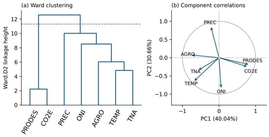
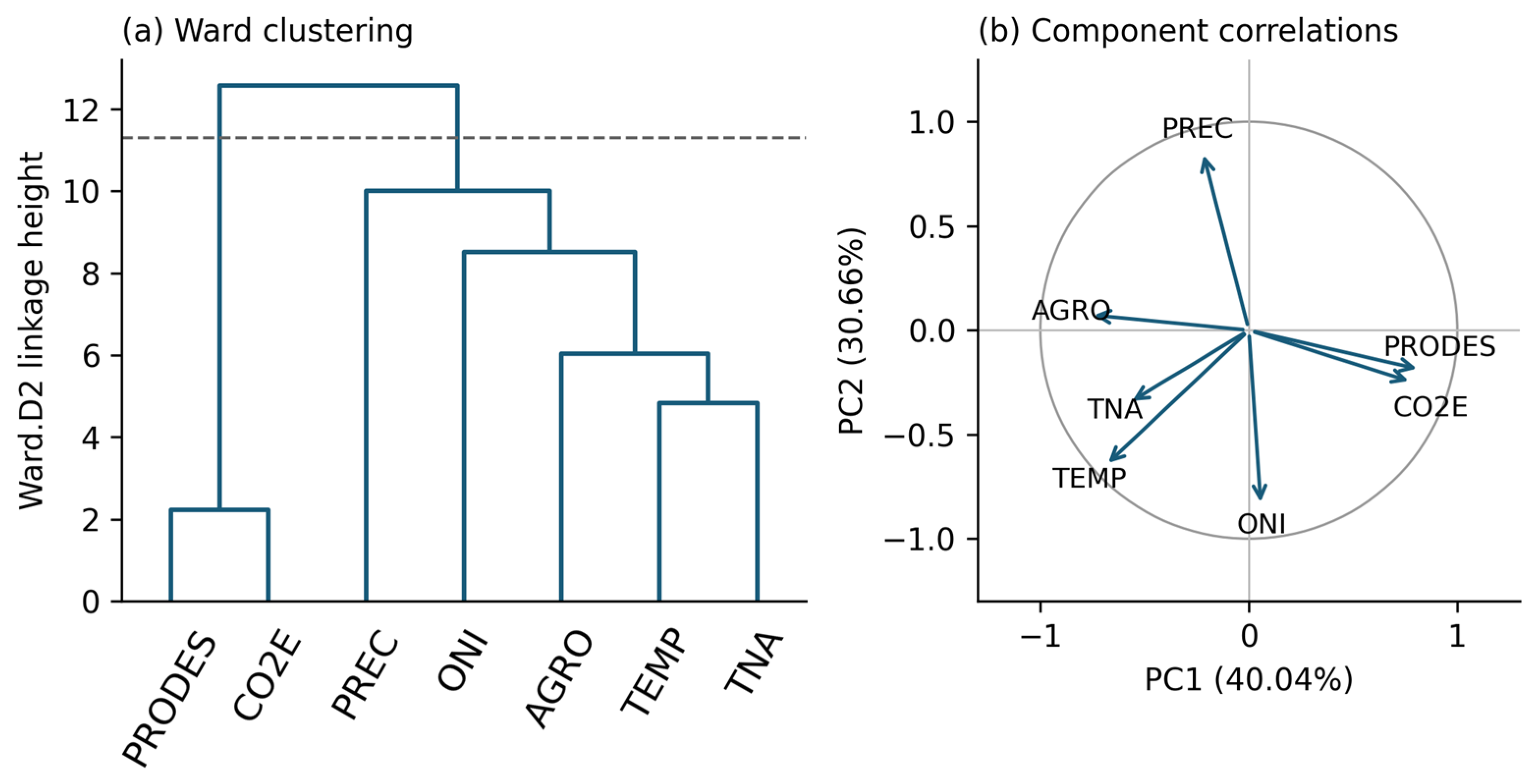
Deforestation and gross emissions form the closest level-series grouping, whereas the climatic and agricultural indicators have a different multivariate configuration. In the level data, the first two principal components explain 40.04% and 30.66% of total standardized variance, respectively, or 70.70% jointly. Both independent-Gaussian and circular-shift parallel analysis retain these two components. Although the third eigenvalue exceeds one (1.122), it does not exceed the corresponding 95th-percentile reference. Ward clustering with silhouette selection gives two groups: PRODES with CO2E and AGRO with TEMP, PREC, ONI, and TNA. Figure 2 summarizes the clustering and component correlations.

Figure 2. Exploratory structure of the seven standardized level series, 1990–2023. (a) Ward.D2 clustering of variables using Euclidean distances; the dashed line marks the silhouette-selected two-group partition. (b) Variable correlations with PC1 and PC2. Component signs are oriented reproducibly; arrows show variable–component correlations.

After differencing PRODES, CO2E, and AGRO and detrending the climate and index series, the first two components explain 67.96% of variance and remain the two retained components. The selected clusters become {ΔPRODES, ΔCO2E, ΔAGRO}, {TEMP, ONI, TNA}, and {PREC}. Agreement between the level and transformed partitions is limited: the adjusted Rand index is 0.16 and pairwise agreement is 0.57. The largest principal angle between the two-component spaces is 44.54°, with mean squared overlap of 0.745. The forest loss–emissions grouping is therefore retained across transformations, while AGRO changes positions and precipitation forms a separate group. These are comparisons of the multivariate structure; response timing is examined below with the BVARX model.

3.3. Stationarity and BVARX Model Selection

Level ADF and PP tests reject a unit root for TEMP, PREC, ONI, and TNA, while trend-KPSS does not reject stationarity for those series (Table 3). Both unit root and stationarity nulls remain unrejected for PRODES, CO2E, and AGRO, leaving their level evidence inconclusive. Break-allowing tests vary with lag choice and do not reject a unit root for these three series at any of the four tested lags. These diagnostics support using first differences for PRODES, CO2E, and AGRO and levels with a trend for the climatic variables; complete tests and transformation sensitivities appear in S2.

Table 3. Primary stationarity tests on level series, 1990–2023.

Variable	ADF	PP	KPSS	ADF Lag	Model Form
PRODES	−1.913	−2.469	0.110	1	First difference
TEMP	−5.207	−5.899	0.066	1	Level with trend
PREC	−5.939	−7.748	0.057	0	Level with trend
CO2E	−1.867	−2.283	0.109	1	First difference
AGRO	−3.363	−2.910	0.134	1	First difference
ONI	−3.660	−4.822	0.072	0	Level with trend
TNA	−3.931	−4.073	0.125	0	Level with trend

All level tests include an intercept and a trend. The 5% critical values are −3.600 for ADF, −3.551 for PP, and 0.146 for KPSS. ADF/PP reject a unit root for statistics below their critical values; KPSS rejects trend stationarity above 0.146. The common ADF candidate window contains 24 regression observations; PP and KPSS bandwidths are three. ONI and TNA enter as controls.

Of the 21 lag–prior specifications, all pass the six global residual checks, 15 also pass the equation-level checks, and 10 are stable positive-lag candidates. Among the latter, BVARX(1) with λ₁ = 5 has the lowest combined normalized RMSE (1.3449) and is retained for dynamic inference (Table 4). The no-lag model has the lowest overall RMSE (1.0429), while the tighter one-lag global screen alternative scores 1.1036. The no-lag model therefore remains the predictive benchmark, and the selected positive-lag model provides the basis for examining propagation across years. Its smallest equation-level screening probability is 0.0524, with a Monte Carlo interval of 0.0462–0.0587, placing its eligibility close to the 5% threshold.

Table 4. Predictive benchmark and leading dynamic specifications.

Role	p	λ1; λ3	RMSE	BICeff	Minimum p
Predictive benchmark	0	—	1.0429	2814.48	0.0520
Global screen dynamic	1	0.1	1.1036	2828.00	0.0300
Primary dynamic	1	5	1.3449	2872.45	0.0524
Best strict p = 2	2	1; 2	1.3925	2885.16	0.2653
Best strict p = 3	3	1; 2	1.3806	2894.49	0.1760

All models use 30 responses for 1994–2023. RMSE averages normalized errors across variables and expanding/rolling schemes for 2011–2023. Minimum p is the smallest bootstrap equation-level Ljung–Box probability. λ₁ controls overall prior tightness; larger values imply weaker shrinkage. λ₃ is inoperative at p = 1. The p = 0 model is not a dynamic candidate. BIC_eff uses the effective parameter count convention in Section 2.4.

The selected model has a largest posterior-mean companion root of 0.4699, and 11,779 out of 12,000 normal–inverse Wishart draws are stable. The minimum effective sample size is 6178, and the maximum split R-hat is 1.0015. S1 reports the complete lag–prior comparison, sampling diagnostics, and parameter counts. The following responses and variance shares use this BVARX(1) model and incorporate innovation covariance uncertainty.

3.4. Dynamic Responses and Forecast Variance Shares

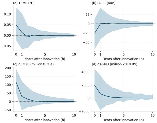
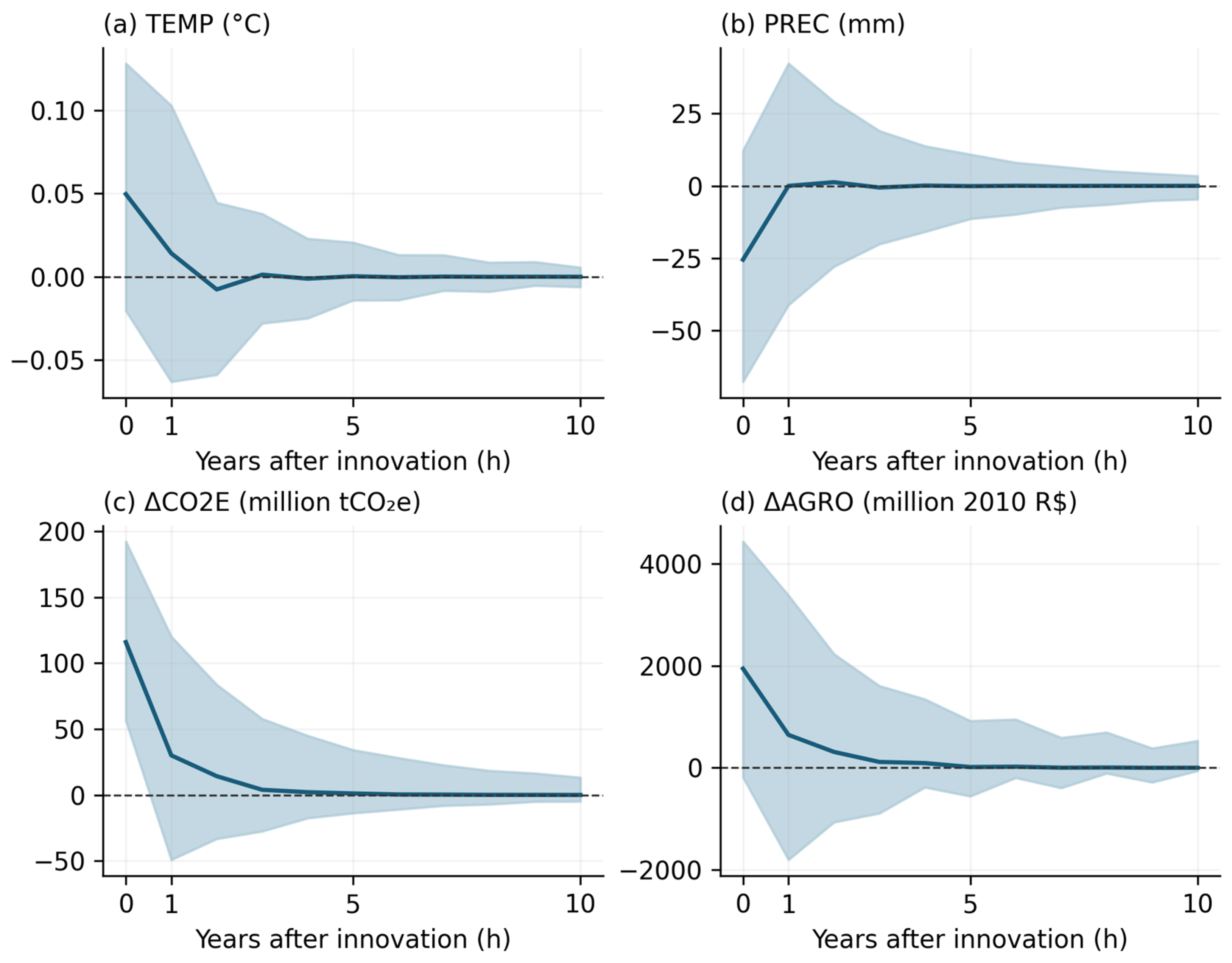
In the selected BVARX(1), the clearest cross-variable response is the positive association between changes in deforestation and gross LULUCF emissions within the same modeled year. The posterior median one standard deviation ΔPRODES innovation is 4186.91 km² (95% credible interval: 3218.31–5766.78 km²). It represents the unexpected component of the annual change in the deforestation rate, conditional on the model. At impact, h = 0, the corresponding ΔCO2E response is 115.87 million tCO₂e (56.33–192.20 million; Table 5).

Table 5. Responses to a positive one standard deviation ΔPRODES innovation.

Response	Unit	Impact, h = 0	One Year, h = 1
ΔPRODES	km2	4186.91 [3218.31, 5766.78]	−587.98 [−2654.72, 1332.99]
TEMP	°C	0.050 [−0.020, 0.128]	0.014 [−0.063, 0.103]
PREC	mm	−25.54 [−67.75, 12.27]	−0.02 [−41.19, 42.34]
ΔCO2E	million tCO2e	115.87 [56.33, 192.20]	30.04 [−49.06, 120.08]
ΔAGRO	BRL million 2010	1943.89 [−186.29, 4436.43]	645.60 [−1800.14, 3378.88]

Posterior medians with 95% pointwise credible intervals in brackets. Primary BVARX(1), λ₁ = 5, independent normal–inverse Wishart posterior conditional on stability, 11,779 draws. Impact shock size varies with the innovation covariance in each draw.

One year later, the median emissions change response is 30.04 million tCO₂e, with a 95% interval of −49.06 to 120.08 million. All subsequent emission response intervals through h = 20 also include zero. Figure 3 shows a detectable contemporaneous association alongside much less precise subsequent responses, leaving its duration unresolved.

Figure 3. Generalized responses to a positive one standard deviation innovation in ΔPRODES under the primary BVARX(1). Dark lines are posterior medians, and shaded areas are 95% pointwise credible intervals from the normal–inverse Wishart posterior conditional on stability. The dashed horizontal line is zero. Impact is h = 0. Emissions and agricultural responses concern annual changes; units are native, with emissions expressed in millions.

The impact temperature median is 0.050 °C (95% interval: −0.020 to 0.128 °C), and the precipitation median is −25.54 mm (−67.75 to 12.27 mm). One year later, the intervals remain broad: −0.063 to 0.103 °C for temperature and −41.19 to 42.34 mm for precipitation (Table 5). Both signs remain compatible with the estimates at each horizon.

The agricultural value-added change has a positive impact median of constant 2010 BRL 1943.89 million, with an interval of −186.29 to 4436.43 million. At h = 1, the median is BRL 645.60 million (−1800.14 to 3378.88 million). The magnitude and direction of the annual agricultural association therefore remain uncertain.

Deforestation innovations account for a normalized median share of 24.06% of emission forecast error variance at H = 1 and 22.22% at H = 5, with a five-year interval of 8.73–33.77% (Table 6). The H = 20 median is 22.26% (8.61–34.03%). The similar shares across horizons and sizeable impact-only share show that contemporaneous covariance contributes substantially to the variance allocation.

Table 6. Normalized variance shares associated with ΔPRODES innovations (%).

Variable	H = 1	H = 5	H = 10	H = 20
TEMP	4.87 [0.02, 16.98]	7.47 [0.65, 20.79]	7.54 [0.66, 21.11]	7.56 [0.66, 21.36]
PREC	4.40 [0.02, 15.68]	7.01 [0.62, 19.61]	7.11 [0.63, 20.21]	7.13 [0.63, 20.52]
ΔCO2E	24.06 [8.86, 34.82]	22.22 [8.73, 33.77]	22.25 [8.62, 33.91]	22.26 [8.61, 34.03]
ΔAGRO	7.53 [0.07, 19.64]	9.51 [0.94, 22.27]	9.60 [0.96, 22.74]	9.61 [0.96, 22.94]

Posterior medians and 95% pointwise credible intervals; primary normal–inverse Wishart posterior conditional on stability. H = 1 includes impact only. Shares are normalized within each draw. H = 20 is a model-dependent long-horizon sensitivity summary.

Across temperature, precipitation, emissions, and agricultural activity, all 80 cross-variable response intervals at h = 1–20 include zero. At H = 20, the median variance shares for TEMP, PREC, and ΔAGRO are 7.56%, 7.13%, and 9.61%, respectively, with broad overlapping intervals (Table 6). The results do not distinguish a most persistent response or a clear ordering of the climatic and agricultural variance shares.

3.5. Sensitivity and Complementary Diagnostics

Across 19 sensitivity specifications, all 71 available one-year cross-variable intervals contain zero. These comparisons include smaller systems, alternative annual windows, removal of TNA or the trend, agricultural accounting controls and transformations, a territorial share emissions adjustment, temperature differencing, and an extension through 2024 without AGRO. They use a fixed innovation covariance, so the covariance uncertainty analysis remains the reference for impact intervals. Magnitudes differ across lag and prior settings; complete comparisons appear in S1 and S2.

None of the 60 conditional Granger tests survives Holm or Benjamini–Hochberg adjustment, and none of the 20 own-ARX stability tests survives Holm adjustment. Thus the auxiliary tests provide no multiplicity-adjusted evidence of directional annual predictability or own-equation parameter changes. Together with the response intervals, these results leave delayed climatic and agricultural associations unresolved.

4. Discussion

4.1. Forest Loss and the Interpretation of Carbon Emissions

The exploratory analyses identify a close relationship between deforestation and gross LULUCF emissions that remains visible after transformation, while the broader climatic and agricultural configuration changes. The BVARX then locates the clearest forest loss–emissions association within the same modeled year. Together, these findings show that the regional indicators share a detectable annual land conversion signal, whereas their later hydroclimatic and agricultural relationships are less precisely resolved. The contribution lies in comparing these dimensions within a common temporal framework and quantifying the uncertainty surrounding their different response patterns.

The emissions measure helps explain the close contemporaneous relationship. Gross LULUCF inventories assign emissions to land transitions using mapped changes and carbon stock assumptions. SEEG 13 combines MapBiomas collection 10 transitions and deforestation/regeneration information [26], linking the inventory to the land change processes monitored by PRODES. The estimated 115.87 million tCO₂e response therefore quantifies co-movement between forest loss and inventory indicators. Their related land change information limits the independence of this evidence, and the model does not identify a causal effect of an externally imposed clearance.

Amazonian carbon studies examine several parts of this environmental process. Gatti et al. evaluate net land–atmosphere carbon exchange, while Aragão et al. examine drought-related fires that can offset reductions in deforestation emissions [7,8]. These findings place the present gross inventory association within a broader carbon balance involving combustion, degradation, uptake, and land cover transitions. Joint monitoring of forest loss and inventories can characterize land conversion pressure, while atmospheric and fire observations provide information about additional carbon processes.

The emissions association is most clearly resolved at impact, with subsequent intervals spanning zero. Its duration consequently remains uncertain at annual regional resolution. The normalized emissions variance share of 22.22% at five years summarizes forecast uncertainty accumulated from impact onward, including the strong initial covariance. This combination—a detectable same-year association and uncertain later responses—defines the temporal contribution of the study.

4.2. Climatic Regulation at Different Spatial and Temporal Scales

The temperature and precipitation intervals leave the magnitude and duration of regional annual responses unresolved. Forest–climate relationships documented at other scales offer context for this limited precision. Weng et al. show that land use change can influence water availability through downwind connections [3]; such connections extend beyond administrative boundaries. Leite-Filho et al. find rainfall responses that depend on the spatial extent of forest loss, with implications for agricultural revenues [4]. A single annual regional average combines these spatially varied interactions.

Spatially resolved observations of warming also measure a different dimension of forest–climate interaction [41]. Land surface temperature contrasts, dry season conditions, and annual regional 2 m air temperature capture different responses. Regional averaging can dilute localized warm or dry anomalies, while annual precipitation totals do not describe rainfall timing relative to agricultural demand. These scale differences offer plausible explanations for limited aggregate precision, although the mechanisms are not separately tested in this model.

For environmental monitoring, the results support combining annual regional indicators with spatially matched forest cover, rainfall, and temperature observations at agriculturally relevant seasons. This combination would connect land conversion pressure more closely to climatic regulation and local exposure, which remain unresolved in the present annual system.

4.3. Agricultural Activity and Ecosystem Service Trade-Offs

Agricultural value added introduces an economic dimension, but its uncertain responses leave the direction of the annual forest loss–activity relationship unresolved. The regional aggregate combines production and changes in activity composition on recently converted and previously cleared land. Macedo et al. document a period in which soy production increased while deforestation declined in southern Amazonia [11]; studies of environmental policy and rural credit likewise show that forest loss responds to economic and institutional conditions [9,10]. These findings help explain why agricultural output and annual clearing need not move proportionally. Establishing regional decoupling would require evidence beyond the imprecise response estimates obtained here.

Agriculture also depends on climatic regulation, which the value-added series does not directly measure. The rainfall–revenue relationships examined by Leite-Filho et al. illustrate a pathway through which land conversion can influence production [4]. Assessing that trade-off requires economic outcomes to be linked to the location, timing, and environmental consequences of conversion. The accounting transition and the broader geographic coverage of AGRO further limit this comparison in the current dataset.

Spatial scenario studies provide a complementary perspective on these trade-offs. In İzmir, Karadeniz et al. combine land cover mapping, MLP–Markov projections, and benefit transfer valuation to assess agricultural and urban transformation alongside ecosystem service changes [42]. In Fethiye, Karadeniz et al. combine spatial land change modeling with InVEST habitat quality under alternative development pathways [43]. These approaches examine how the location and configuration of conversion shape ecological outcomes. Combined with historical evidence on annual associations, spatially explicit analyses can connect regional change to particular landscapes and services. Their numerical findings remain specific to their study regions and scenario assumptions.

4.4. Scope and Limitations

This study assesses relationships among forest loss, emissions, hydroclimate, and agricultural activity at the regional annual scale. Aggregation may obscure local differences and seasonal processes. Comparability across indicators is affected by geographic coverage, observation windows, and the agricultural accounting transition. Related land change information underlying PRODES and the emissions inventory also informs the interpretation of their contemporaneous association.

The common sample of 30 annual observations limits the precision of delayed responses, and the no-lag benchmark provides better conditional forecasts than the selected dynamic model. Sensitivity analyses assess several data and specification choices, while posterior intervals remain conditional on the selected model and stability restriction. The estimates therefore characterize regional co-movement, with limited evidence about persistence. Investigating local mechanisms and causal effects requires finer-scale observations and identification strategies that address climatic and socioeconomic confounding.

5. Conclusions

The annual regional evidence for 1990–2023 identifies a positive contemporaneous association between changes in Amazon deforestation and gross LULUCF emissions. The relationship is retained across exploratory transformations and quantified in a dynamic model with oceanic climate controls. A one standard deviation deforestation change innovation is associated with an emissions change response of 115.87 million tCO₂e (95% credible interval: 56.33–192.20 million), reflecting the annual land conversion information shared by forest loss and inventory indicators.

The objectives of identifying co-movement and quantifying associated forecast variance shares were achieved. The timing and persistence objective was partly achieved: the emissions association is resolved within the same year, while subsequent emissions, temperature, precipitation, and agricultural responses remain too uncertain to establish their direction or duration. The normalized emissions variance share is 22.22% at five years, with a 95% interval of 8.73–33.77%; it includes the contemporaneous contribution.

The environmental contribution is a common assessment of the annual relationships linking forest loss, emissions, hydroclimate, and agricultural activity showing where regional monitoring provides a clear signal and where additional resolution is needed. The findings support joint tracking of deforestation and gross emissions, complemented by spatial and seasonal climate and agricultural observations to assess climatic regulation and vulnerability. Such integration can better connect regional land conversion indicators to the environmental conditions supporting agricultural production.

References

- IPCC. Climate Change 2021: The Physical Science Basis. Contribution of Working Group I to the Sixth Assessment Report of the Intergovernmental Panel on Climate Change; Masson-Delmotte, V., Zhai, P., Pirani, A., Connors, S.L., Péan, C., Berger, S., Caud, N., Chen, Y., Goldfarb, L., Gomis, M.I., et al., Eds.; Cambridge University Press: Cambridge, UK, 2021. [Google Scholar] [CrossRef] [Scilit]
- Spracklen, D.V.; Arnold, S.R.; Taylor, C.M. Observations of increased tropical rainfall preceded by air passage over forests. Nature 2012, 489, 282–285. [Google Scholar] [CrossRef] [Scilit] [PubMed]
- Weng, W.; Luedeke, M.K.B.; Zemp, D.C.; Lakes, T.; Kropp, J.P. Aerial and surface rivers: Downwind impacts on water availability from land use changes in Amazonia. Hydrol. Earth Syst. Sci. 2018, 22, 911–927. [Google Scholar] [CrossRef] [Scilit]
- Leite-Filho, A.T.; Soares-Filho, B.S.; Davis, J.L.; Abrahão, G.M.; Börner, J. Deforestation reduces rainfall and agricultural revenues in the Brazilian Amazon. Nat. Commun. 2021, 12, 2591. [Google Scholar] [CrossRef] [Scilit] [PubMed]
- Marengo, J.A.; Espinoza, J.-C.; Fu, R.; Jiménez-Muñoz, J.C.; Alves, L.M.; da Rocha, H.R.; Schöngart, J. Long-term variability, extremes and changes in temperature and hydrometeorology in the Amazon region: A review. Acta Amaz. 2024, 54, e54es22098. [Google Scholar] [CrossRef] [Scilit]
- Zemp, D.C.; Schleussner, C.-F.; Barbosa, H.M.J.; Rammig, A. Deforestation effects on Amazon forest resilience. Geophys. Res. Lett. 2017, 44, 6182–6190. [Google Scholar] [CrossRef] [Scilit]
- Aragão, L.E.O.C.; Anderson, L.O.; Fonseca, M.G.; Rosan, T.M.; Vedovato, L.B.; Wagner, F.H.; Silva, C.V.J.; Silva Junior, C.H.L.; Arai, E.; Aguiar, A.P.; et al. 21st century drought-related fires counteract the decline of Amazon deforestation carbon emissions. Nat. Commun. 2018, 9, 536. [Google Scholar] [CrossRef] [Scilit] [PubMed]
- Gatti, L.V.; Basso, L.S.; Miller, J.B.; Gloor, M.; Gatti Domingues, L.; Cassol, H.L.G.; Tejada, G.; Aragão, L.E.O.C.; Nobre, C.; Peters, W.; et al. Amazonia as a carbon source linked to deforestation and climate change. Nature 2021, 595, 388–393. [Google Scholar] [CrossRef] [Scilit] [PubMed]
- Assunção, J.; Gandour, C.; Rocha, R. Deforestation slowdown in the Brazilian Amazon: Prices or policies? Environ. Dev. Econ. 2015, 20, 697–722. [Google Scholar] [CrossRef] [Scilit]
- Assunção, J.; Gandour, C.; Rocha, R.; Rocha, R. The effect of rural credit on deforestation: Evidence from the Brazilian Amazon. Econ. J. 2020, 130, 290–330. [Google Scholar] [CrossRef] [Scilit]
- Macedo, M.N.; DeFries, R.S.; Morton, D.C.; Stickler, C.M.; Galford, G.L.; Shimabukuro, Y.E. Decoupling of deforestation and soy production in the southern Amazon during the late 2000s. Proc. Natl. Acad. Sci. USA 2012, 109, 1341–1346. [Google Scholar] [CrossRef] [Scilit] [PubMed]
- Marengo, J.A.; Espinoza, J.C. Extreme seasonal droughts and floods in Amazonia: Causes, trends and impacts. Int. J. Climatol. 2016, 36, 1033–1050. [Google Scholar] [CrossRef] [Scilit]
- Franco, M.A.; Rizzo, L.V.; Teixeira, M.J.; Artaxo, P.; Azevedo, T.; Lelieveld, J.; Nobre, C.A.; Pöhlker, C.; Pöschl, U.; Shimbo, J.; et al. How climate change and deforestation interact in the transformation of the Amazon rainforest. Nat. Commun. 2025, 16, 7944. [Google Scholar] [CrossRef] [Scilit] [PubMed]
- Attílio, L.A. Amazon deforestation and CO2 emissions: A macroeconomic approach using the GVAR. J. Reg. Sci. 2025, 65, 189–220. [Google Scholar] [CrossRef] [Scilit]
- Barreto, A.C.; Martins, T.; Souza, A.M. Modeling deforestation drivers in the Brazilian Amazon: A comparison of quantitative approaches. Big Earth Data 2025, 9, 1023–1057. [Google Scholar] [CrossRef] [Scilit]
- Mendonça, M.J.; Loureiro, P.R.A.; Sachsida, A. The dynamics of land-use in Brazilian Amazon. Ecol. Econ. 2012, 84, 23–36. [Google Scholar] [CrossRef] [Scilit]
- Litterman, R.B. Forecasting with Bayesian vector autoregressions—Five years of experience. J. Bus. Econ. Stat. 1986, 4, 25–38. [Google Scholar] [CrossRef] [Scilit]
- Giannone, D.; Lenza, M.; Primiceri, G.E. Prior selection for vector autoregressions. Rev. Econ. Stat. 2015, 97, 436–451. [Google Scholar] [CrossRef] [Scilit]
- Koop, G.; Korobilis, D. Bayesian multivariate time series methods for empirical macroeconomics. Found. Trends Econom. 2010, 3, 267–358. [Google Scholar] [CrossRef] [Scilit]
- Pesaran, H.H.; Shin, Y. Generalized impulse response analysis in linear multivariate models. Econ. Lett. 1998, 58, 17–29. [Google Scholar] [CrossRef] [Scilit]
- Instituto Nacional de Pesquisas Espaciais (INPE). TerraBrasilis: PRODES Deforestation Rates, Legal Amazon. Available online: https://terrabrasilis.dpi.inpe.br/app/dashboard/deforestation/biomes/legal_amazon/rates (accessed on 14 October 2026).
- Muñoz-Sabater, J.; Dutra, E.; Agustí-Panareda, A.; Albergel, C.; Arduini, G.; Balsamo, G.; Boussetta, S.; Choulga, M.; Harrigan, S.; Hersbach, H.; et al. ERA5-Land: A state-of-the-art global reanalysis dataset for land applications. Earth Syst. Sci. Data 2021, 13, 4349–4383. [Google Scholar] [CrossRef] [Scilit]
- Copernicus Climate Change Service (C3S). ERA5-Land Monthly Averaged Data from 1950 to Present; Climate Data Store: Reading, UK, 2019. [Google Scholar] [CrossRef]
- Instituto Brasileiro de Geografia e Estatística (IBGE). Amazônia Legal: Limites e Municípios, 2024. Available online: https://www.ibge.gov.br/geociencias/cartas-e-mapas/mapas-regionais/15819-amazonia-legal.html (accessed on 14 October 2026).
- Funk, C.; Peterson, P.; Landsfeld, M.; Pedreros, D.; Verdin, J.; Shukla, S.; Husak, G.; Rowland, J.; Harrison, L.; Hoell, A.; et al. The climate hazards infrared precipitation with stations—A new environmental record for monitoring extremes. Sci. Data 2015, 2, 150066. [Google Scholar] [CrossRef] [Scilit] [PubMed]
- Sistema de Estimativas de Emissões e Remoções de Gases de Efeito Estufa (SEEG). Nota Metodológica SEEG 13: Mudança de Uso da Terra e Floresta, Brasil. 2025. Available online: https://seeg.eco.br/wp-content/uploads/2026/01/SEEG13-NM-MUT-BR.pdf (accessed on 14 October 2026).
- Instituto de Pesquisa Econômica Aplicada (IPEA). Ipeadata: Agricultural Gross Value Added at Basic Prices by State, Million Constant 2010 Reais. Available online: https://www.ipeadata.gov.br/Default.aspx (accessed on 12 October 2026).
- NOAA Climate Prediction Center. Oceanic Niño Index, Version 5. Available online: https://www.cpc.ncep.noaa.gov/products/analysis_monitoring/enso/oni/v5/ (accessed on 29 October 2026).
- NOAA Physical Sciences Laboratory. Tropical North Atlantic Index, HadISST1.1, 1991–2020 Climatology. Available online: https://psl.noaa.gov/data/correlation/tna.data (accessed on 12 October 2026).
- Ward, J.H. Hierarchical grouping to optimize an objective function. J. Am. Stat. Assoc. 1963, 58, 236–244. [Google Scholar] [CrossRef]
- Jolliffe, I.T.; Cadima, J. Principal component analysis: A review and recent developments. Philos. Trans. R. Soc. A 2016, 374, 20150202. [Google Scholar] [CrossRef] [Scilit]
- Horn, J.L. A rationale and test for the number of factors in factor analysis. Psychometrika 1965, 30, 179–185. [Google Scholar] [CrossRef] [Scilit] [PubMed]
- Dickey, D.A.; Fuller, W.A. Distribution of the estimators for autoregressive time series with a unit root. J. Am. Stat. Assoc. 1979, 74, 427–431. [Google Scholar] [CrossRef] [Scilit]
- Phillips, P.C.B.; Perron, P. Testing for a unit root in time series regression. Biometrika 1988, 75, 335–346. [Google Scholar] [CrossRef]
- Kwiatkowski, D.; Phillips, P.C.B.; Schmidt, P.; Shin, Y. Testing the null hypothesis of stationarity against the alternative of a unit root. J. Econom. 1992, 54, 159–178. [Google Scholar] [CrossRef] [Scilit]
- Zivot, E.; Andrews, D.W.K. Further evidence on the great crash, the oil-price shock, and the unit-root hypothesis. J. Bus. Econ. Stat. 1992, 10, 251–270. [Google Scholar] [CrossRef] [Scilit]
- Lütkepohl, H. New Introduction to Multiple Time Series Analysis; Springer: Berlin/Heidelberg, Germany, 2005. [Google Scholar] [CrossRef]
- Holm, S. A simple sequentially rejective multiple test procedure. Scand. J. Stat. 1979, 6, 65–70. [Google Scholar]
- Benjamini, Y.; Hochberg, Y. Controlling the false discovery rate: A practical and powerful approach to multiple testing. J. R. Stat. Soc. B 1995, 57, 289–300. [Google Scholar] [CrossRef] [Scilit]
- Zeileis, A.; Leisch, F.; Hornik, K.; Kleiber, C. strucchange: An R package for testing for structural change in linear regression models. J. Stat. Softw. 2002, 7, 1–38. [Google Scholar] [CrossRef] [Scilit]
- Butt, E.W.; Baker, J.C.A.; Bezerra, F.G.S.; von Randow, C.; Aguiar, A.P.D.; Spracklen, D.V. Amazon deforestation causes strong regional warming. Proc. Natl. Acad. Sci. USA 2023, 120, e2309123120. [Google Scholar] [CrossRef] [Scilit] [PubMed]
- Karadeniz, E.; Sajjad, M.; Sunbul, F.; Yüksel Kaya, A.; Deniz Adıgüzel, A.; Ozel, H.B. Urban and agricultural land transformation and ecosystem service trade-offs in İzmir, Türkiye (1985–2075). Eur. J. Remote Sens. 2026, 59, 2723518. [Google Scholar] [CrossRef] [Scilit]
- Karadeniz, E.; Adıgüzel, F.; Zhang, M.; Wei, X.; Özel, H.U.; Özel, H.B. Modeling tourism-driven coastal land-use change and habitat quality under alternative development pathways: Implications for environmental management from explainable AI. Ocean Coast. Manag. 2026, 282, 108356. [Google Scholar] [CrossRef] [Scilit]
Disclaimer/Publisher’s Note: The statements, opinions and data contained in all publications are solely those of the individual author(s) and contributor(s) and not of MDPI and/or the editor(s). MDPI and/or the editor(s) disclaim responsibility for any injury to people or property resulting from any ideas, methods, instructions or products referred to in the content. |
© 2026 by the authors. Licensee MDPI, Basel, Switzerland. This article is an open access article distributed under the terms and conditions of the Creative Commons Attribution (CC BY) license.