Predicting BOD₅ Removal Efficiency in a Constructed Wetland from Satellite and Meteorological Data Using Interpretable Machine Learning

Abstract

Constructed wetlands (CWs) offer a low-cost and sustainable option for wastewater treatment, but their performance is commonly assessed through infrequent, periodic field sampling that yields temporally sparse records. This study evaluated whether five-day biochemical oxygen demand (BOD₅) removal efficiency at the Gložan horizontal subsurface-flow constructed wetland (Serbia) could be predicted from freely available satellite-derived and meteorological variables alone, using an interpretable machine learning workflow. Sixteen candidate predictors—the mean and spatial standard deviation of Landsat-derived indices (land surface temperature [LST], Normalized Difference Vegetation Index [NDVI], Normalized Difference Water Index [NDWI], Normalized Difference Suspended Sediment Index [NDSSI], Modified NDWI [MNDWI], and chlorophyll index) together with 7- and 14-day air temperature and precipitation—were screened against 38 BOD₅ removal-efficiency observations (n = 38; 2005–2026) using Pearson correlation and three Random Forest importance measures, refined through variance-inflation-factor analysis and regularization-guided elimination, and evaluated across twelve regression algorithms under nested leave-one-out cross-validation (LOOCV). A one-component Partial Least Squares (PLS) regression using four predictors—14-day mean air temperature, spatial variability of land surface temperature (LST), and the mean and spatial variability of the Normalized Difference Water Index (NDWI)—achieved the best performance in the external (outer-loop LOOCV) evaluation (RMSE = 5.73 percentage points, MAE = 4.37 percentage points, R² = 0.41). Linear-family models consistently outperformed tree-ensemble and kernel-based methods, and the explicit removal of multicollinearity during predictor selection was key to this advantage, allowing the linear models to surpass their nonlinear counterparts. These results indicate that a compact set of satellite-derived and meteorological variables can provide meaningful and interpretable information on CW treatment performance without in situ operational data, offering a complement to—rather than a replacement for—traditional physicochemical analyses in the monitoring of constructed wetlands.

1. Introduction

Constructed wetlands (CWs) are nature-based wastewater-treatment systems that use interacting physical, chemical, and biological processes to remove organic matter and other pollutants [1]. Because of their relatively low construction and operating costs, limited energy requirements, and ecological co-benefits, they are particularly suitable for small and medium-sized settlements, where conventional treatment infrastructure may be economically or operationally impractical and where the technical personnel and laboratory capacity required for routine effluent analysis are frequently limited [2,3]. In such settings, cost-effective and low-maintenance approaches for tracking treatment performance are of direct practical value to the utilities and local authorities responsible for regulatory compliance and long-term system management. CW treatment performance nevertheless varies over time in response to hydraulic conditions, meteorological variability, vegetation development, microbial community dynamics, and operational factors [3]. A meta-analysis comparing surface-flow, subsurface-flow, and hybrid CWs reported satisfactory BOD removal across all system types, with hybrid systems showing the highest overall efficiency [4]. Reliable monitoring of this variability is therefore important for evaluating treatment efficiency and supporting long-term system management.

Five-day biochemical oxygen demand (BOD₅) is widely used as an indicator of the biodegradable organic matter content of wastewater, while the reduction in BOD₅ between influent and effluent is commonly used to evaluate treatment efficiency [5]. This assessment is conventionally based on periodic collection and laboratory analysis of paired influent and effluent samples. Although such measurements provide direct and reliable information on treatment performance, periodic sampling produces temporally sparse records [6] and offers little insight into spatial variability within the wetland. This limitation is particularly pronounced for horizontal subsurface-flow constructed wetlands (HSSF CWs). In surface-flow systems, the free water surface is exposed, so that its extent, turbidity, algal growth, and vegetation cover can be observed directly and captured by optical remote sensing as comparatively unambiguous indicators of surface condition. In HSSF systems, by contrast, wastewater flows below the substrate surface and is never directly visible from above; the treatment-relevant processes and the hydraulic disturbances that affect them—such as clogging, preferential flow, and short-circuiting—develop within the porous medium and are expressed at the surface only indirectly, for example, through the moisture status and vigour of the overlying vegetation. Consequently, both direct visual inspection and remote observation of HSSF wetlands are inherently more indirect than for surface-flow systems, and internal hydraulic and treatment processes cannot be assessed without dedicated field campaigns. Existing methods for investigating system condition, including hydraulic tests, tracer studies, geophysical surveys, and direct substrate sampling, generally require specialized equipment or invasive measurements [7,8,9].

Satellite remote sensing offers a complementary, non-invasive approach for characterizing the surface conditions of CWs without continuous field deployment [10]. Optical and thermal imagery can provide repeated information on vegetation condition, surface and vegetation moisture, inundation patterns, and land surface temperature. Across both natural and artificial water systems, remotely sensed data have increasingly been combined with empirical, analytical, and machine learning retrieval methods to estimate optically active and, more recently, optically inactive water-quality parameters, including turbidity, chlorophyll-a, suspended matter, dissolved oxygen, and oxygen-demand indicators [11,12]. Such approaches have been applied not only to lakes, rivers, and reservoirs but also to engineered systems, including constructed wetlands, where satellite imagery has been used to assess vegetation status and treatment context [10,13]. In the present study, a compact set of well-established spectral indices was selected to represent the specific surface processes hypothesized to be linked to treatment performance, rather than to maximize the number of candidate predictors: the Normalized Difference Vegetation Index (NDVI) and a chlorophyll index for vegetation vigour and biomass; the Normalized Difference Water Index (NDWI) and the Modified NDWI (MNDWI) for canopy and surface water content and inundation extent; the Normalized Difference Suspended Sediment Index (NDSSI) for surface turbidity and suspended-sediment signals; and land surface temperature (LST) for the thermal state of the wetland surface. These indices were prioritized over more specialized or sensor-specific alternatives because they are physically interpretable and can be computed from the standard Landsat spectral bands available consistently across the full study period, which supports both temporal continuity and transferability to other sites and archives [14,15,16].

The use of Landsat imagery nevertheless imposes spatiotemporal constraints that are directly relevant to routine CW monitoring. A single Landsat sensor revisits a given location only every 16 days, and a substantial proportion of these acquisitions is rendered unusable by cloud cover, haze, and cirrus contamination, so that the number of cloud-free scenes coincident with field sampling is limited. In addition, the 30 m spatial resolution of the optical and shortwave-infrared bands—and the coarser native resolution of the thermal band, resampled to 30 m—is large relative to the dimensions of individual wetland cells, which restricts the spatial detail that can be resolved within the system. These limitations motivated the use of cell-aggregated index statistics, specifically the spatial mean and spatial standard deviation of each index, rather than fine-grained spatial mapping, and they define the temporal resolution at which satellite-based observation can realistically complement field sampling.

Machine learning approaches have previously been applied to predict pollutant removal in CWs using influent concentrations, hydraulic loading, retention time, substrate properties, and other operational measurements [17]. Tomenko et al. [18] compared multiple regression analysis against multilayer perceptron and radial basis function networks for predicting biochemical oxygen demand in subsurface-flow constructed wetlands, while Akratos et al. [17] developed neural network models and design equations for BOD and COD removal in HSSF systems specifically. Gou and Cui [19] compared nine machine learning algorithms for free-water-surface CWs, identifying random forest and extra trees as the preferred models. Kumar et al. [20] compared multiple linear regression, artificial neural networks, support vector machines, and random forest for predicting total phosphorus removal in hybrid CWs. Li et al. [21] developed a fully connected neural network that combined weather conditions with influent and effluent water-quality and flow data to simulate treatment performance in a Phragmites australis-planted HSSF CW.

These studies demonstrate the capacity of machine learning to represent the complex and frequently nonlinear relationships that arise from the coupled physical, chemical, and microbial processes governing CW treatment. They share, however, a common dependence on field-based operational and water-quality inputs—such as influent and effluent concentrations, hydraulic loading, or retention time—that can be obtained only through the same in situ sampling that such models are ultimately intended to support. This dependence constrains their usefulness as a complement to conventional monitoring, because the required predictors are unavailable in the absence of routine field measurement. The specific gap addressed in the present study is therefore whether BOD₅ removal efficiency can be estimated from freely available satellite-derived and meteorological variables alone—without any in situ operational or water-quality inputs—and whether this can be achieved through an interpretable modelling workflow rather than the black-box neural-network architectures that have predominated in earlier work.

Predicting treatment performance from satellite-derived and meteorological variables also entails distinct methodological challenges. Environmental monitoring datasets are frequently constrained by limited sample sizes, which increase the risk of overfitting when flexible models are applied [22]. Remotely sensed indices calculated from overlapping spectral bands may exhibit substantial multicollinearity [23], and the relationships between environmental predictors and CW treatment performance may themselves be complex and potentially nonlinear [24,25]. Under these conditions, highly flexible algorithms may overfit the available observations, whereas simpler or regularized models may yield more stable and interpretable predictions. Robust model development therefore requires careful predictor screening and multicollinearity assessment, appropriate model tuning and unbiased validation, comparison of models spanning a range of complexity, and interpretation of the final model [26,27,28,29].

This study develops and evaluates an interpretable machine learning workflow for predicting BOD₅ removal efficiency at the Gložan HSSF constructed wetland in Serbia using satellite-derived and meteorological predictors alone. The workflow combines linear and nonlinear predictor-ranking methods, variance-inflation-factor analysis, regularization-guided sequential predictor refinement, and nested leave-one-out cross-validation; twelve regression algorithms representing linear, regularized, kernel-based, instance-based, probabilistic, and tree-ensemble approaches were evaluated within a common validation framework. The specific objectives were to: (i) identify the most informative satellite-derived and meteorological predictors of BOD₅ removal efficiency; (ii) reduce predictor redundancy and multicollinearity within this candidate set; (iii) compare the predictive performance of the twelve algorithms under small-sample conditions; and (iv) interpret the direction and relative importance of the variables retained in the final model. Consistent with these objectives, we hypothesized that spatial heterogeneity in the surface thermal and moisture conditions of the wetland, together with recent meteorological conditions, carries information about its biological treatment efficiency, such that BOD₅ removal efficiency can be predicted from freely available satellite-derived and meteorological variables in the absence of in situ data, and, further, that increasing model complexity would not improve predictive performance once predictor redundancy had been systematically addressed. Establishing whether such a low-cost, satellite- and meteorology-based approach can provide meaningful information on treatment performance is of particular relevance to the small and medium-sized settlements in which CWs are most commonly deployed and in which monitoring resources are most limited.

2. Materials and Methods

2.1. Study Area

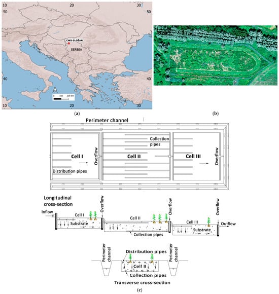
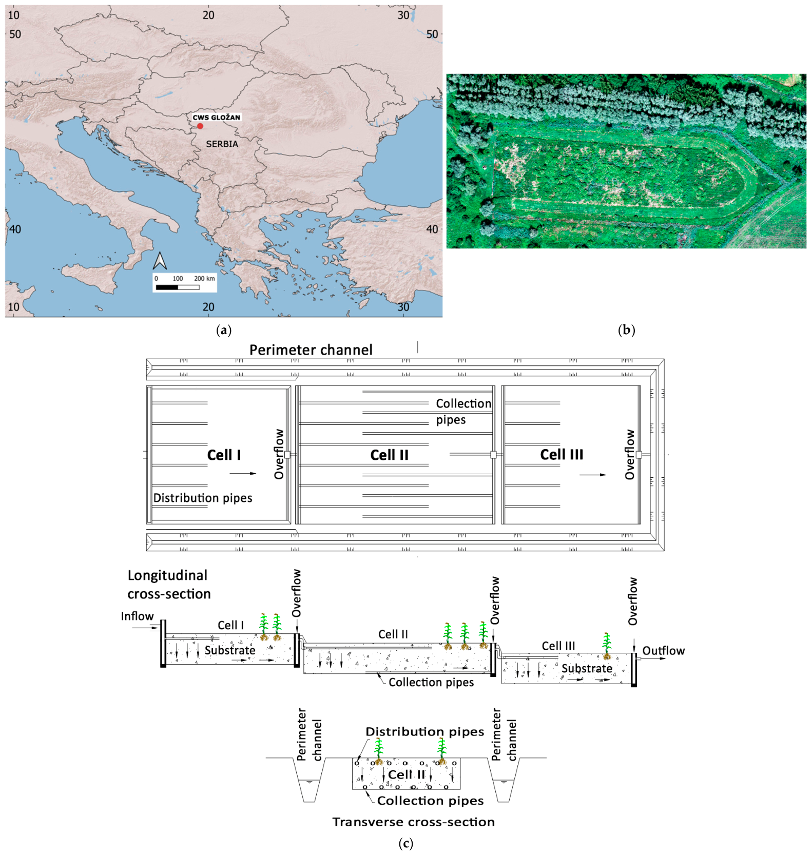
The study was conducted on a constructed wetland system (CWS) for wastewater treatment of the Gložan settlement. Gložan settlement (Figure 1) is located in the north-western part of Serbia (45.27° N, 19.57° E) and is an urbanized settlement in the Pannonian Basin, with around 2000 inhabitants [30,31]. Based on the geographical location, the climate conditions could be characterized as moderate continental climate with significant year-round precipitation, dry winters, and a secondary precipitation peak in autumn [32].

Figure 1. Location of the constructed wetland system (CWS) in Gložan (a), an aerial view of the site (b), and a schematic of the Gložan horizontal subsurface-flow constructed wetland (c).

The constructed wetland system (CWS) in Gložan is a horizontal subsurface-flow type and consists of three cells with a total area of 9400 m². Individual cell surface areas are 2000 m² (Cell I), 5000 m² (Cell II), and 2400 m² (Cell III). The system utilizes reed (Phragmites australis (Cav.) Trin. ex Steud.) as a biofilter, a species that naturally occurred at the site prior to the construction of the CWS. Wastewater treatment is achieved by sequential flow through the three cells, with hydraulic retention times of 24, 48, and 33 h in Cells I, II, and III, respectively. The treated effluent is discharged into a canal connected to the Danube River [30,31]. Further details on the design, operation, and treatment performance of the Gložan constructed wetland are available in previous studies [33,34,35,36,37].

2.2. Water-Quality Data

Data on five-day biochemical oxygen demand (BOD₅) were obtained from field measurements, relevant literature [30,31], and responsible stakeholders through technical and professional cooperation established within the framework of the Horizon Europe DALIA and SWIM projects. The dataset comprised 38 observations of BOD₅ measured at the inlet and outlet of the CWS over the period 2005–2026. Samples were collected regularly, generally four times per year during the study period; however, only 38 samples were used in this study. Because sampling was distributed across the year, the dataset spans all four seasons over the 2005–2026 period and therefore captures seasonal variability in influent characteristics and treatment performance. Sampling dates were selected based on the availability of satellite images of adequate quality, specifically cloud-free images covering the constructed wetland area. Sampling and sample handling prior to analysis were carried out in accordance with the relevant standards (SRPS ISO 5667-10, SRPS EN ISO 5667-1, and SRPS EN ISO 5667-3) [38,39,40]. The samples consisted of time-proportional composites. The analyses were performed in the accredited laboratory of the Department of Chemistry, Faculty of Sciences, University of Novi Sad. BOD₅ was determined by the manometric (respirometric) method according to the laboratory’s accredited internal method H1.002. BOD₅ removal efficiency was calculated as (C_in − C_out)/C_in × 100, where C_in and C_out represent inlet and outlet BOD₅ concentrations, respectively [41,42]. Removal efficiency was evaluated on an integrated, whole-system basis, from the single system inlet to the final outlet, and therefore reflects the combined performance of the three cells operating in series (combined hydraulic retention time ≈ 105 h) rather than per-cell removal. For the selected sampling events, the mean BOD₅ removal efficiency was 90.6%, with values ranging from 72% to 99%. Influent BOD₅ over this period ranged from 107 to 780 mg/L (mean 325 mg/L) and effluent BOD₅ from 3.5 to 143 mg/L (mean 31 mg/L).

2.3. Satellite-Derived Indices and Variables

Landsat Collection 2 Level-2 surface-reflectance and surface-temperature products were used. Optical bands were rescaled using the product-specific scale and offset factors, while surface temperature was converted from Kelvin to degrees Celsius. Clouds, cirrus, snow, and cloud shadows were masked using the QA_PIXEL quality-assessment band of the Landsat Collection 2 Level-2 products, removing pixels flagged for cirrus (bit 2), cloud (bit 3), cloud shadow (bit 4), or snow (bit 5) and retaining only pixels clear on all four flags. A scene-level cloud-cover filter (below 50%) was additionally applied, and all index statistics were computed only over the unmasked pixels within the wetland boundary. For each BOD₅ sampling date, the image closest to the sampling date within the ±15-day window and satisfying the cloud-cover criterion was selected. The ±15-day window represents a compromise between the Landsat revisit interval (16 days for a single sensor, further reduced by cloud loss) and the temporal scale of the surface predictors, which reflect vegetation, moisture, and thermal conditions that vary on seasonal rather than daily scales; given the combined hydraulic retention time of the system (approximately 105 h), this window captures conditions representative of each sampling event while retaining a sufficient number of cloud-free scenes. Of the 38 selected scenes, 21 were acquired before the corresponding sampling date, 16 after, and one on the same day, with a mean absolute temporal offset of approximately 6.9 days; all scenes were acquired within ±15 days of sampling. The complete list of sampling dates, image acquisition dates, and corresponding day differences is provided in Table S1 of the Supplementary Materials.

Satellite-derived indices and variables were calculated from Landsat 5, Landsat 7, Landsat 8, and Landsat 9 imagery in Google Earth Engine (GEE). Mean values and spatial standard deviations among pixels were calculated within the CW boundary to represent average conditions and within-wetland spatial variability, respectively. These statistics were obtained using region reducers at a 30 m analysis scale. In the Landsat image projection used for the regional reduction, the wetland polygon comprised approximately ten valid 30 m pixels, and this number was identical across all 38 cloud-free acquisitions used. The larger number of pixels apparently intersecting the wetland polygon in the GEE Code Editor map results from the on-the-fly reprojection and resampling of imagery to the Web Mercator projection (EPSG:3857) used for visualization and does not represent the pixel grid used for the regional statistics. Because only approximately ten pixels contributed to the calculations, the spatial-variability predictors should be interpreted as coarse indicators of within-wetland heterogeneity and remain subject to mixed-pixel, boundary, and geolocation effects. In particular, the thermal data used to derive land surface temperature have a coarser native spatial resolution than the 30 m analysis grid: approximately 120 m for Landsat 5 TM, 60 m for Landsat 7 ETM+, and 100 m for Landsat 8/9 TIRS, with the standard thermal products resampled to 30 m. Consequently, LSTstDev represents spatial variability in resampled thermal data and should not be interpreted as independent 30 m thermal information, whereas the reflective bands used to calculate optical indices, including NDWI, have a native spatial resolution of 30 m. The initial set of Satellite-derived indices and variables included:

• Land surface temperature (LST);
• Normalized Difference Vegetation Index (NDVI);
• Normalized Difference Water Index (NDWI) [11];
• Normalized Difference Suspended Sediment Index (NDSSI);
• Modified Normalized Difference Water Index (MNDWI);
• Green chlorophyll index (CI_green).

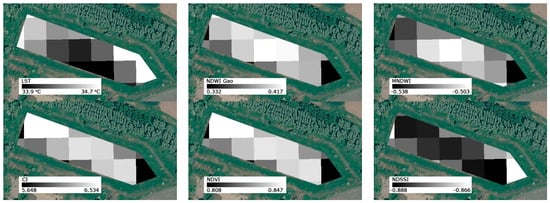
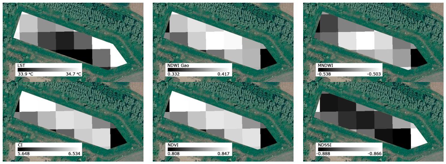
These indices capture thermal conditions, vegetation dynamics, and surface or vegetation moisture, which are critical drivers of wetland functioning [3,15,16]. Representative grayscale maps of LST and the selected spectral indices for the Gložan constructed wetland on 10 July 2025 are presented in Figure 2. In the equations below, Blue, Green, Red, NIR, and SWIR1 refer to surface reflectance measured in the blue, green, red, near-infrared, and first shortwave-infrared portions of the electromagnetic spectrum, respectively. These spectral regions respond differently to vegetation, water, moisture, and suspended material, allowing the corresponding surface characteristics to be emphasized through band combinations.

Figure 2. Grayscale visualizations of LST, Gao’s NDWI, MNDWI, CI, NDVI, and NDSSI for the Gložan constructed wetland on 10 July 2025. Each image was independently displayed using a 100% minimum–maximum stretch based on the range of pixel values within the study area. This stretch was applied only for visualization of the grayscale maps and does not affect the mean and standard-deviation index statistics used in the modelling.

LST [43], derived from thermal infrared satellite data, was considered as a proxy for thermal conditions in the CWS area, governing microbial activity, biochemical reaction rates, and oxygen dynamics relevant to BOD₅ removal.

NDVI, calculated as (NIR − Red)/(NIR + Red) [14], was considered to represent vegetation density and photosynthetic activity, reflecting primary productivity and organic matter dynamics that regulate microbial processes within the system.

NDWI, calculated as (NIR − SWIR)/(NIR + SWIR) [15], was considered as an indicator of vegetation water content and moisture conditions, linked to plant physiological status, evapotranspiration, and moisture-driven microbial activity.

NDSSI, calculated as (Blue − NIR)/(Blue + NIR) [44], was considered as a proxy for suspended sediment and turbidity conditions, influencing light penetration and related ecological processes.

MNDWI, calculated as (Green − SWIR1)/(Green + SWIR1) [45], was considered as a proxy for surface water distribution and hydrological conditions, controlling flow dynamics, hydraulic retention time, and microbial degradation processes.

CI_green, calculated as (NIR/Green) − 1 [46], was considered as an indicator of vegetation vigour and chlorophyll content, reflecting primary productivity, organic matter inputs, and associated microbial activity.

2.4. Meteorological Data

Daily meteorological parameters, specifically air temperature and precipitation, were retrieved from the European Climate Assessment & Dataset (ECA&D), a robust, quality-controlled repository for European climate research [47,48,49]. Meteorological data were obtained from a gridded dataset with a spatial resolution of 0.1° (approximately 10 km). Data from the grid cell covering the Gložan constructed wetland were used in the analysis. This grid cell corresponds to the site location (45.27° N, 19.57° E) and provides area-averaged air-temperature and precipitation values at the native 0.1° resolution of the ECA&D E-OBS gridded product. To evaluate the short-term influence of weather conditions on treatment efficiency, the following aggregated indicators were calculated:

• 7-day and 14-day mean air temperatures;
• 7-day and 14-day cumulative precipitation.

2.5. Machine Learning Modelling

To identify the most robust framework for predicting BOD₅ removal efficiency at the Gložan constructed wetland, twelve candidate machine learning models were evaluated. This comparative approach was adopted to assess both linear and nonlinear relationships between the satellite-derived indices, meteorological variables, and treatment performance.

Multiple Linear Regression (MLR): MLR models the relationship between a response variable and multiple predictors by fitting a linear equation to the observed data. The response is estimated as a linear combination of the predictor variables [50].

Partial Least Squares Regression (PLS): PLS transforms the original predictors into a smaller number of latent components that maximize covariance with the response variable, thereby enabling regression in the presence of correlated predictors [51].

Ridge Regression applies an L2 penalty, based on the sum of squared coefficients, which shrinks coefficient estimates toward zero and can improve model stability in the presence of multicollinearity [52]. Lasso Regression applies an L1 penalty, based on the sum of the absolute coefficient values, and can shrink some coefficients exactly to zero, thereby performing automatic predictor selection [53].

Elastic Net Regression: Elastic Net combines the L₁ penalty of Lasso with the L₂ penalty of Ridge Regression, allowing simultaneous coefficient shrinkage and predictor selection. The balance between these two penalties is governed by a tuning parameter α ∈ [0, 1], where α = 1 corresponds to pure Lasso regression and α = 0 reduces to pure Ridge Regression [54].

Random Forest (RF): RF constructs multiple decision trees using bootstrap samples and random subsets of predictors, and averages their predictions to produce the final estimate. It can model nonlinear relationships and interactions and can also provide measures of predictor importance [55].

Extra Trees Regression: Extra Trees is an ensemble method that constructs multiple highly randomized decision trees and averages their predictions. Compared with Random Forest, it introduces additional randomness into the selection of split thresholds, which can reduce model variance and improve robustness [56].

Gradient Boosting Regression: Gradient Boosting builds an ensemble of decision trees sequentially, with each new tree fitted to reduce the prediction errors made by the preceding ensemble [57].

Extreme Gradient Boosting (XGBoost): XGBoost is an optimized implementation of gradient-boosted decision trees that incorporates regularization, shrinkage, and subsampling to improve predictive performance and computational efficiency [58].

Support Vector Regression (SVR): SVR estimates a regression function while allowing prediction errors within a predefined tolerance. Through the use of kernel functions, it can represent both linear and nonlinear relationships while controlling model complexity [59,60].

K-Nearest Neighbours Regression (KNN): KNN is a nonparametric method that predicts the response of a new observation from the responses of the most similar observations in the predictor space. Its performance depends on the number of neighbours, the weighting scheme, and the distance metric, all of which were optimized during model tuning [61].

Gaussian Process Regression (GPR): GPR is a probabilistic, kernel-based approach that models the response as a distribution over possible functions and can represent smooth nonlinear relationships while quantifying predictive uncertainty [62].

2.5.1. Data Preprocessing, Model Tuning, and Validation

Predictors were standardized before fitting scale-sensitive models, including MLR, Ridge, Lasso, Elastic Net, PLS, SVR, KNN, and GPR. Standardization used the z-score transformation (zero mean and unit standard deviation) and was embedded in each model’s pipeline, so that the standardization parameters were estimated only from the training observations within each cross-validation fold, preventing information leakage. Tree-based models were fitted without predictor standardization. Model performance was assessed using a nested Leave-One-Out Cross-Validation (LOOCV) framework. Model hyperparameters were optimized using grid search within an inner leave-one-out cross-validation loop. Predictive performance was evaluated in an outer leave-one-out cross-validation loop, ensuring that the held-out observation was not used during hyperparameter selection. This framework is particularly suitable for small datasets because it maximizes the use of the available observations while reducing optimistic bias associated with hyperparameter selection [28]. In the outer loop, each of the 38 observations was held out once as the test case; for the corresponding training set of 37 observations, hyperparameters were tuned by grid search within an inner leave-one-out loop using RMSE as the selection criterion, imputation and standardization were refit within each fold, and the tuned model predicted the single held-out observation. The 38 outer-loop predictions were then pooled for performance evaluation.

Predictor relevance was initially assessed using four complementary measures selected to capture both linear and nonlinear/interaction-based associations: absolute Pearson correlation with BOD₅ removal efficiency, and three importance measures derived from a Random Forest model—mean decrease in impurity (MDI) [55], permutation importance [55], and mean absolute SHAP (SHapley Additive exPlanations) value [63,64]. Predictors were ranked separately using each measure, and the mean rank across the four methods was used to define an initial reduced predictor set. This initial set comprised the eight highest-ranked variables (the top half of the sixteen candidates), a deliberately inclusive cut-off intended only to pass a manageable, consistently high-ranking group to the subsequent, more stringent steps; the final predictors were determined by the variance-inflation-factor analysis and regularization-guided elimination that followed rather than by this cut-off, and the outcome was not sensitive to its exact value. To assess the robustness of predictor and model selection under the small sample size, a bootstrap stability analysis (1000 resamples) was additionally performed and is reported in the Supplementary Materials. Multicollinearity was assessed using variance inflation factors (VIFs) [65] calculated from the predictor correlation matrix. Sequential refinement was subsequently performed by examining coefficient shrinkage in Lasso and Elastic Net models. Predictors with coefficients equal to or close to zero were removed sequentially, and all twelve models were re-evaluated after each refinement step.

Model performance was assessed using the coefficient of determination (R²), root mean square error (RMSE), and mean absolute error (MAE), calculated from the pooled outer-loop LOOCV predictions. These were computed as:

$$\mathit{RMSE}=\sqrt{\left({\displaystyle \frac{1}{n}}\right){\sum }_i{\left(y_i-\widehat{y_i}\right)}^2}$$

(1)

$$\mathit{MAE}=\left({\displaystyle \frac{1}{n}}\right){\sum }_i\left|y_i-\widehat{y_i}\right|$$

(2)

where yᵢ and ŷᵢ are the observed and predicted BOD₅ removal efficiencies expressed in percentage points and n = 38; R² was obtained from the same pooled predictions. Higher R² values indicate better predictive performance, whereas lower RMSE and MAE values indicate smaller prediction errors. Because BOD₅ removal efficiency was expressed as a percentage, RMSE and MAE are reported in percentage points. Adjusted R² was additionally calculated as a descriptive measure during predictor refinement to account for differences in the number of predictors:

$$R_{\mathit{adj}}^2=1-(1-R^2){\displaystyle \frac{n-1}{n-p-1}}$$

(3)

where n is the number of observations and p is the number of predictors included in the model.

2.5.2. Modelling Workflow

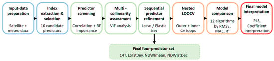
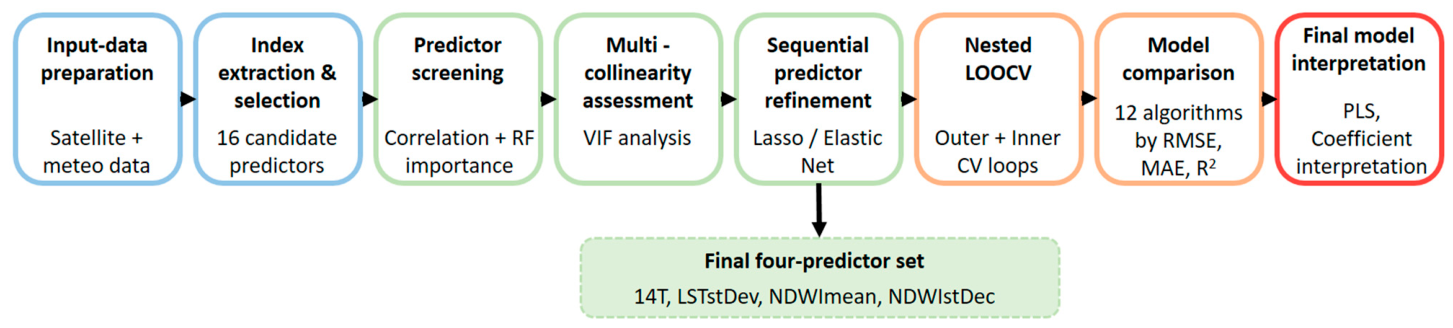
The complete modelling workflow, including input-data preparation, index extraction and selection, predictor screening, multicollinearity assessment, sequential predictor refinement, nested LOOCV, model comparison, and final model interpretation, is summarized in Figure 3.

Figure 3. General modelling workflow for predicting BOD₅ removal efficiency using satellite-derived and meteorological data.

3. Results and Discussion

3.1. Predictor Selection

The initial candidate predictor set comprised 16 remote-sensing and meteorology-derived variables: mean and standard deviation of Land Surface Temperature (LSTmean, LSTstDev), Normalized Difference Vegetation Index (NDVImean, NDVIstDev), Normalized Difference Water Index [11] (NDWImean, NDWIstDev), Normalized Difference Suspended Sediment Index (NDSSImean, NDSSIstDev), Modified Normalized Difference Water Index (MNDWImean, MNDWIstDev), and Green Chlorophyll Index (CImean, CIstDev), together with 7-day and 14-day mean air temperature (7T, 14T) and cumulative precipitation (7P, 14P). The ranking of all sixteen candidate predictors across the four diagnostics is summarized in Table 1.

Table 1. All 16 candidate predictors ranked by Pearson correlation and three Random Forest-based importance measures (rank in parentheses), sorted by mean rank across the four methods.

Predictor	Pearson r (Rank)	RF MDI (Rank)	Permutation (Rank)	SHAP (Rank)	Mean Rank
7T	−0.549 (5)	0.231 (1)	1.463 (1)	1.783 (1)	2.00
LSTmean	−0.599 (1)	0.157 (3)	0.682 (3)	1.079 (3)	2.50
NDWImean	−0.573 (3)	0.057 (5)	0.296 (5)	0.486 (5)	4.50
LSTstDev	−0.348 (12)	0.162 (2)	1.107 (2)	1.154 (2)	4.50
NDWIstDev	0.421 (9)	0.070 (4)	0.323 (4)	0.530 (4)	5.25
14T	−0.576 (2)	0.056 (6)	0.202 (8)	0.402 (6)	5.50
NDSSImean	0.570 (4)	0.039 (8)	0.144 (11)	0.277 (8)	7.75
7P	−0.303 (13)	0.044 (7)	0.259 (6)	0.335 (7)	8.25
NDSSIstDev	−0.365 (10)	0.028 (10)	0.180 (9)	0.236 (10)	9.75
NDVImean	−0.484 (7)	0.027 (11)	0.121 (12)	0.122 (12)	10.50
MNDWImean	0.113 (15)	0.031 (9)	0.174 (10)	0.215 (11)	11.25
MNDWIstDev	0.033 (16)	0.023 (13)	0.216 (7)	0.256 (9)	11.25
CImean	−0.545 (6)	0.017 (14)	0.087 (14)	0.079 (15)	12.25
NDVIstDev	0.349 (11)	0.026 (12)	0.115 (13)	0.106 (13)	12.25
CIstDev	−0.471 (8)	0.016 (15)	0.054 (16)	0.084 (14)	13.25
14P	−0.171 (14)	0.014 (16)	0.080 (15)	0.071 (16)	15.25

Consensus ranking across the four methods (Table 1) identified eight predictors with the lowest (best) mean ranks—7T, LSTmean, NDWImean, LSTstDev, NDWIstDev, 14T, NDSSImean, and 7P (mean rank 2.00–8.25)—which were carried forward as the initial candidate set for model development. The remaining eight predictors—NDSSIstDev, NDVImean, MNDWImean, MNDWIstDev, CImean, NDVIstDev, CIstDev, and 14P (mean rank 9.75–15.25)—ranked consistently lower across all four methods and were excluded from further consideration.

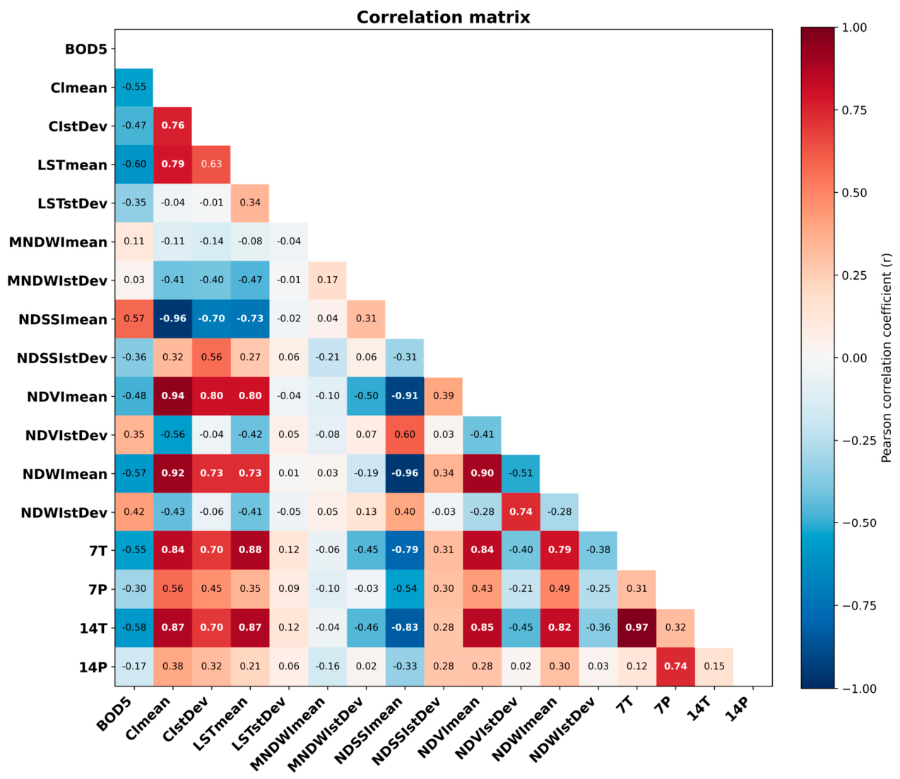
Two notable discrepancies emerged between the correlation-based and Random Forest-based rankings. First, 7T and LSTstDev ranked comparatively low based on Pearson correlation (ranks 5 and 12, respectively) but ranked first and second across all three Random Forest-based importance measures, suggesting the presence of nonlinear relationships or interaction effects not captured by linear correlation. Whereas the Pearson coefficient reflects only the strength of a linear association, the Random Forest-based measures also detect nonlinear and interaction effects; in addition, 7T is nearly collinear with 14T (r = 0.969), which further reduces its unique linear signal. Second, CImean, CIstDev, and NDSSImean showed the opposite pattern, exhibiting moderate-to-strong linear correlations with BOD₅ removal efficiency but comparatively low Random Forest-based importance. This pattern suggests that these variables may provide information largely redundant with that contained in the more strongly retained predictors, rather than representing a genuine lack of predictive value. In particular, although NDSSImean correlated appreciably with removal efficiency (r = 0.57), it was highly collinear with NDWImean (|r| = 0.90–0.96; VIF = 45) and showed low Random Forest importance, so its information was largely redundant; it was subsequently shrunk to near zero and removed during refinement without any loss of performance.

3.1.1. Multicollinearity Assessment

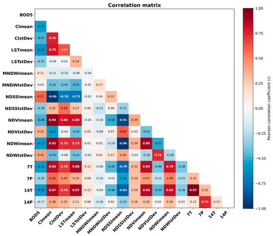
To evaluate this redundancy hypothesis, variance inflation factors (VIFs) were computed for all 16 candidate predictors (Table 2) from their pairwise correlation matrix (Figure 4). Severe multicollinearity (VIF > 10) was identified among CImean (VIF = 64.3), NDSSImean (45.4), NDVImean (31.2), NDWImean (30.1), 14T (27.3), and 7T (23.1), reflecting a single dominant thermal/optical cluster in which pairwise correlations reached |r| = 0.70–0.97. In particular, 7T and 14T were nearly collinear (r = 0.969), and CImean, NDSSImean, and NDVImean were each highly collinear with NDWImean (|r| = 0.90–0.96). By contrast, LSTstDev (VIF = 2.69), NDWIstDev (3.88), 7P (3.87), and NDSSIstDev (2.79) exhibited relatively low multicollinearity with the other candidate predictors. This finding is consistent with the earlier observation that the Random Forest-based importance of these variables was unlikely to result primarily from information shared with other predictors. The very high VIFs within the optical/chlorophyll group arise because these indices are computed from overlapping spectral bands and respond to the same underlying vegetation signal, making them nearly interchangeable; including several together inflates variance and destabilizes the coefficients without adding independent information, which motivated reducing the cluster to a single representative (NDWImean).

Table 2. Variance inflation factors (VIFs) for all 16 candidate predictors.

Predictor	VIF	Predictor	VIF
CImean	64.29	NDVIstDev	8.46
NDSSImean	45.44	14P	3.91
NDVImean	31.20	NDWIstDev	3.88
NDWImean	30.05	7P	3.87
14T	27.32	MNDWIstDev	3.82
7T	23.14	NDSSIstDev	2.79
LSTmean	12.01	LSTstDev	2.69
CIstDev	9.26	MNDWImean	1.35

Figure 4. Pearson correlation matrix of the 16 candidate predictors and their correlations with BOD₅ removal efficiency.

3.1.2. Sequential Refinement

Based on the combined evidence from importance ranking, VIFs, and domain plausibility, an initial reduced set of eight predictors was selected for model development: 7T, LSTmean, LSTstDev, NDWImean, NDWIstDev, NDSSImean, 7P, and 14T. Using this eight-predictor set, twelve regression approaches were evaluated: Multiple Linear Regression, Partial Least Squares Regression, Ridge Regression, Lasso Regression, Elastic Net, Random Forest, Extra Trees, XGBoost, Gradient Boosting, Support Vector Regression, K-Nearest Neighbours, and Gaussian Process Regression. All models were evaluated under the nested LOOCV framework described in Section 2.5.1, with performance estimated from the outer-loop predictions.

With the initial eight-predictor set, K-Nearest Neighbours provided the best performance, with an outer-loop LOOCV RMSE of 5.96, an MAE of 4.41, an R² of 0.36, and an adjusted R² of 0.19. Examination of the Lasso coefficients indicated that NDSSImean, 7T, and LSTmean contributed little independent predictive information, with all three exhibiting coefficients equal to or near zero (specifically, magnitudes below 0.004). These predictors were therefore removed sequentially, and all twelve models were re-evaluated after each step. The 0.004 value is an empirical near-zero cut-off applied to the standardized coefficients; the final predictor set was insensitive to its precise value within a reasonable range. The resulting five-predictor set—LSTstDev, NDWImean, NDWIstDev, 7P, and 14T—was best modelled using Ridge Regression and achieved an RMSE of 5.93, an MAE of 4.47, an R² of 0.37, and an adjusted R² of 0.27. Both Lasso and Elastic Net subsequently indicated that 7P contributed little additional predictive information. After its removal, the final four-predictor set—LSTstDev, NDWImean, NDWIstDev, and 14T—produced the best overall performance under the nested LOOCV framework. Partial Least Squares Regression achieved an RMSE of 5.73, an MAE of 4.37, an R² of 0.41, and an adjusted R² of 0.34 (Table 3).

Table 3. Summary of the sequential predictor-refinement process.

Stage	Predictor Set	Best Model	RMSE	MAE	R2	Adj. R2	Lasso/EN Shrinkage
1	7T, LSTmean, LSTstDev, NDWImean, NDWIstDev, NDSSImean, 7P, 14T	KNN	5.96	4.41	0.36	0.19	NDSSImean, 7T, LSTmean ≈ 0
2	LSTstDev, NDWImean, NDWIstDev, 7P, 14T	Ridge	5.93	4.47	0.37	0.27	7P ≈ 0
3 (final)	LSTstDev, NDWImean, NDWIstDev, 14T	PLS	5.73	4.37	0.41	0.34	—

Outer-loop LOOCV RMSE decreased progressively during predictor refinement, from 5.958 for the initial eight-predictor set to 5.926 for the five-predictor set and 5.731 for the final four-predictor set. Cross-validated R² likewise increased from 0.363 to 0.369 and finally to 0.410. MAE remained relatively stable across the first two stages, increasing slightly from 4.409 to 4.473, before decreasing to its lowest value of 4.366 for the final model. Adjusted R² also increased monotonically (0.188 → 0.270 → 0.338). Overall, the final four-predictor set provided the best balance between predictive performance and model simplicity.

The final retained predictor set—LSTstDev, NDWImean, NDWIstDev, and 14T—captures four largely distinct dimensions of information: mean air temperature (14T), spatial variability in land surface temperature (LSTstDev), and the mean level and spatial variability of vegetation water content (NDWImean and NDWIstDev, respectively). Variance inflation factors recalculated for the final predictor set confirmed substantially reduced multicollinearity (Table 4), supporting its suitability for comparative evaluation across all twelve regression models.

Table 4. Variance inflation factors within the final four-predictor set.

Predictor	VIF
14T	3.41
NDWImean	3.20
NDWIstDev	1.15
LSTstDev	1.04

3.2. Model Comparison and Predictive Performance

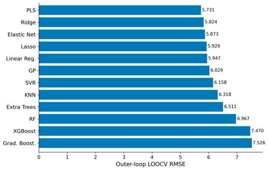
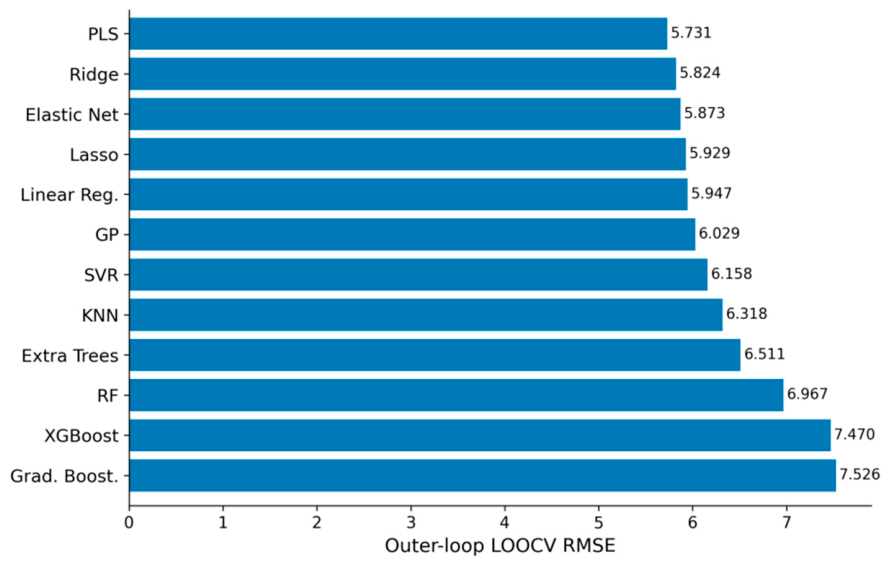
Twelve regression algorithms were evaluated using the final four-predictor set (LSTstDev, NDWImean, NDWIstDev, and 14T) within a nested Leave-One-Out Cross-Validation (LOOCV) framework. Hyperparameters were optimized through grid search in the inner LOOCV loop, thereby reducing information leakage associated with hyperparameter tuning. Model performance, ranked according to the RMSE obtained from the outer LOOCV loop, is summarized in Table 5 and Figure 5.

Table 5. Outer-loop LOOCV performance of twelve regression models for predicting BOD₅ removal efficiency at the Gložan constructed wetland (n = 38; 4 predictors).

Rank	Model	RMSE	MAE	R2
1	PLS Regression	5.731	4.366	0.410
2	Ridge	5.824	4.399	0.390
3	Elastic Net	5.873	4.420	0.380
4	Lasso	5.929	4.535	0.368
5	Linear Regression	5.947	4.559	0.364
6	Gaussian Process	6.029	4.610	0.347
7	SVR	6.158	4.652	0.318
8	KNN	6.318	4.833	0.282
9	Extra Trees	6.511	4.840	0.238
10	Random Forest	6.967	5.097	0.128
11	XGBoost	7.470	5.394	−0.003
12	Gradient Boosting	7.526	5.627	−0.018

Figure 5. Comparison of the predictive performance of the twelve regression models based on outer-loop leave-one-out cross-validation RMSE. Lower RMSE indicates better predictive performance.

A clear and consistent pattern emerged: the five linear-family models—PLS Regression, Ridge Regression, Elastic Net, Lasso Regression, and Multiple Linear Regression—occupied the top five positions, whereas all tree-based ensemble methods—Random Forest, Extra Trees, XGBoost, and Gradient Boosting—ranked in the lower half of the comparison. Notably, XGBoost and Gradient Boosting produced negative outer-loop LOOCV R² values, indicating poorer predictive performance than a baseline model that predicts the mean observed BOD₅ removal efficiency.

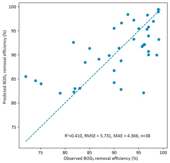
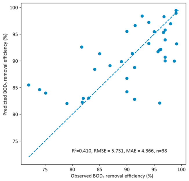
PLS Regression was the best-performing model, achieving an outer-loop LOOCV RMSE of 5.73, an MAE of 4.37, and an R² of 0.41. The inner-loop grid search selected one latent component for the PLS model. It was therefore selected as the final model for coefficient interpretation and further discussion. The agreement between observed and outer-loop LOOCV-predicted BOD₅ removal efficiency for the final PLS regression model is shown in Figure 6.

Figure 6. Observed versus outer-loop LOOCV-predicted BOD₅ removal efficiency for the final PLS regression model. The dashed line represents perfect agreement between observed and predicted values.

Most residuals are small, with the two largest deviations of approximately ±14 percentage points (≈±2.4 SD). The outliers follow a regression-toward-the-mean pattern typical of a single-component linear model: the lowest observed efficiencies (72–79%) are over-predicted and the highest (≈99%) slightly under-predicted. These deviations are not artefacts of temporal mismatch, as all scenes were acquired within the ±15-day window (mean gap ≈ 7 days) and the absolute residual is uncorrelated with the sampling-to-image gap (Pearson r ≈ 0.00); they instead reflect operational or loading factors not observable through surface and meteorological variables.

3.3. PLS Regression Coefficients

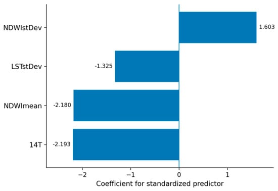
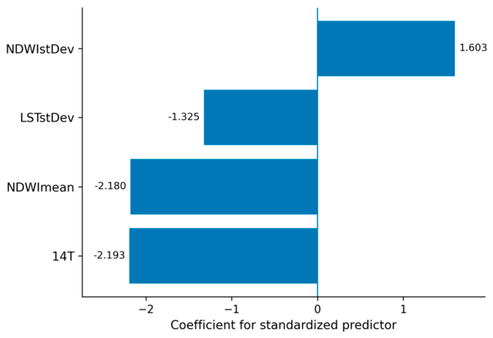
After model selection, the final one-component PLS regression model was refitted to the complete dataset, and the coefficients for the standardized predictors were extracted for interpretation. The single latent component represents one weighted combination of the four predictors that best tracks removal efficiency; physically, it corresponds to a combined thermal–moisture gradient of the wetland surface, indicating that the predictors relate to efficiency mainly along a single shared axis of variation. Their magnitude and direction are presented in Figure 7, with predictors ordered according to coefficient value. Negative coefficients indicate inverse associations with predicted BOD₅ removal efficiency, whereas positive coefficients indicate direct associations.

Figure 7. Coefficients for the standardized predictors in the final one-component PLS regression model refitted to the complete dataset. Positive and negative values indicate positive and inverse associations with predicted BOD₅ removal efficiency, respectively.

The absolute values of the coefficients for the standardized predictors fell within a relatively narrow range (1.3–2.2), suggesting that no single predictor had a markedly stronger association with predicted BOD₅ removal efficiency than the others. The final predictor set also exhibited low multicollinearity, as confirmed in Table 4. Three predictors—14T, NDWImean, and LSTstDev—were inversely associated with predicted BOD₅ removal efficiency, whereas NDWIstDev showed a positive association.

Linear-family models consistently outperformed the nonlinear and ensemble approaches in this dataset. This result may be related to the small sample size and the reduced, low-collinearity predictor set obtained through sequential refinement. With n = 38 and a LOOCV scheme in which each outer fold was trained on only 37 observations, tree-based ensemble methods—Random Forest, Gradient Boosting, XGBoost, and Extra Trees—had limited data from which to derive stable and generalizable partitions of the predictor space. Boosting compounds this limitation by sequentially fitting residuals, which under such small samples amounts to fitting noise, and tree-based models produce piecewise-constant predictions that cannot extrapolate, whereas removal efficiency varies smoothly with the predictors—structure better suited to linear models. The negative outer-loop LOOCV R² values obtained for XGBoost and Gradient Boosting indicate that these models generalized less effectively than a baseline model predicting the mean observed BOD₅ removal efficiency.

This outcome is also consistent with the predictor-selection process. The initial screening used Random Forest-based importance measures—MDI, permutation importance, and SHAP—to identify potential nonlinear and interaction-based associations that might not be captured by Pearson correlation alone, including the relevance of predictors such as LSTstDev. However, after the predictor set was reduced to four variables with low multicollinearity (Table 4), the relationship between the retained predictors and BOD₅ removal efficiency was adequately represented by a linear combination of latent components, which is the type of structure PLS Regression is designed to model. Thus, nonlinear diagnostics were useful during predictor screening, whereas the final predictive relationship did not appear to require the additional flexibility of nonlinear models.

3.4. Interpretation of Predictor Associations with Removal Efficiency

The 14-day mean air temperature (14T) had the largest absolute coefficient in the model, although its magnitude was very similar to that of NDWImean. Its negative coefficient indicated that higher air temperatures were associated with lower BOD₅ removal efficiency. Although higher temperatures may enhance microbial degradation kinetics, several counteracting mechanisms are plausible in constructed wetlands. Increased evapotranspiration under warmer conditions may alter water levels, hydraulic retention time, and flow patterns [3], and, as is well established, higher water temperatures reduce dissolved-oxygen solubility, which can limit aerobic degradation pathways involved in BOD₅ removal [66].

Mean vegetation and surface moisture content (NDWImean) was also negatively associated with BOD₅ removal efficiency. Higher NDWImean values, reflecting greater vegetation and surface moisture, may indicate wetter or more extensively inundated conditions within the wetland. Such conditions can promote oxygen-limited or anaerobic zones, thereby altering the balance between aerobic and anaerobic treatment processes and potentially reducing the contribution of aerobic organic matter degradation pathways to BOD₅ removal [2,3].

Spatial variability in vegetation and surface moisture (NDWIstDev), calculated as the pixel-to-pixel standard deviation within the wetland extent for each sampling date, was positively associated with BOD₅ removal efficiency. In contrast to NDWImean, which reflects the overall level of vegetation and surface moisture across the wetland, NDWIstDev describes the spatial heterogeneity of these conditions. Greater variability may reflect the coexistence of relatively wetter and drier areas and, consequently, a broader range of oxygen and redox conditions. Such spatial heterogeneity may support complementary treatment processes, including aerobic and anaerobic organic matter degradation and nitrogen transformations in constructed wetlands [67,68,69]. NDWIstDev may therefore provide information on spatial conditions associated with improved BOD₅ removal compared with more uniform moisture conditions. Furthermore, the weak correlations between NDWIstDev and the other retained predictors suggest that its association with BOD₅ removal efficiency reflects largely independent information rather than substantial overlap with the other predictors.

Spatial variability in land surface temperature (LSTstDev), in contrast, showed a negative association with BOD₅ removal efficiency, suggesting that greater thermal heterogeneity across the wetland may be associated with reduced treatment performance. Spatially uneven thermal conditions may reflect differences in vegetation cover, inundation, water depth, or hydraulic flow, potentially creating zones with different microbial activity and organic matter degradation rates. Such spatial variation may contribute to less uniform treatment conditions and lower overall system efficiency [3]. LSTstDev exhibited relatively low multicollinearity with the other candidate predictors throughout the diagnostic process (VIF = 2.69) and consistently ranked among the most important predictors across all three Random Forest-based importance measures, despite its comparatively weak linear correlation with BOD₅ removal efficiency. These findings suggest that LSTstDev captures a distinct aspect of the spatial thermal structure of the wetland.

Although NDWIstDev and LSTstDev both describe spatial variability within the wetland, their opposite associations with BOD₅ removal efficiency are not necessarily contradictory. In brief, moisture heterogeneity diversifies redox conditions in a way that favours removal, whereas thermal heterogeneity signals hydraulic non-uniformity that reduces treatment consistency. The two variables capture different spatial characteristics and were only weakly correlated with one another. NDWIstDev primarily reflects heterogeneity in vegetation and moisture conditions, which may indicate a mosaic of wetter and drier zones and a broader range of redox environments. By contrast, LSTstDev reflects thermal heterogeneity, which may be associated with uneven vegetation cover, patchy inundation, stagnant areas, or non-uniform hydraulic conditions, including possible hydraulic short-circuiting. Such conditions may reduce flow uniformity and treatment consistency compared with a more thermally homogeneous system characterized by relatively uniform vegetation cover and inundation. However, the mechanisms underlying these associations cannot be determined from remote-sensing data alone and should be investigated further by combining vegetation and thermal imagery with direct measurements of water depth, dissolved oxygen, vegetation density, and hydraulic flow patterns.

The final model showed moderate predictive performance, with an outer-loop LOOCV R² of 0.410, indicating that the four retained remote-sensing and meteorological predictors captured a meaningful, although incomplete, proportion of the observed variation in BOD₅ removal efficiency. This result should be interpreted in the context of the indirect nature of the prediction task. The biological processes reflected by BOD₅ removal efficiency are driven by hydraulic, chemical, and microbial factors that cannot be directly observed via remote sensing. The model should therefore be regarded as a useful but partial predictive representation rather than a comprehensive mechanistic description of treatment performance. Earlier machine learning studies of constructed wetlands generally report higher predictive accuracy, but they rely on in situ operational and water-quality inputs such as influent and effluent concentrations, hydraulic loading, and retention time [17,18,19,20,21]. Because the present model uses only freely available satellite and meteorological data—a more indirect task constrained by a small field record (n = 38)—an outer-loop R² of 0.41 is expected and still informative, its value lying in the accessibility and field-independence of the inputs.

This level of performance should also be read in the context of the target variable. BOD₅ is a non-optically active parameter with no direct spectral signature and can therefore only be inferred indirectly, which fundamentally constrains the accuracy achievable from remote sensing. Reported R² for such parameters spans a wide range: multispectral, independently validated retrievals are typically modest—for example, best-model R² of 0.36–0.52 for dissolved oxygen, permanganate index, total nitrogen, and total phosphorus [70]—whereas hyperspectral retrievals with in situ reflectance calibration can exceed 0.8 [71], and the limitations of retrieving these parameters are well documented [72]. The present value of 0.41 falls within the lower part of this range, consistent with a deliberately conservative design that uses only freely available satellite and meteorological data, without optically active proxies or concurrent reflectance calibration, predicts removal efficiency rather than concentration, relies on a small field record, and is evaluated under leakage-free nested cross-validation. Interpreted together with the low absolute errors (RMSE and MAE of 5.73 and 4.37 percentage points, approximately 6.3% and 4.8% of the mean removal efficiency), the model provides practically useful screening information rather than a definitive quantitative prediction.

Because the approach requires no in situ sampling, it could serve operators of small municipal systems as a low-cost screening tool between laboratory analyses—for example, flagging periods when reduced efficiency is more likely and prompting targeted sampling. It is best regarded as decision support rather than a replacement for accredited analysis, given its moderate accuracy, the 16-day revisit interval, and the need for site-specific calibration.

The relatively small sample size (n = 38) further limits the precision and stability of model estimates and may have disadvantaged the more flexible nonlinear models included in the comparison. Future research based on a longer monitoring record and additional hydrological and operational covariates, such as measured hydraulic retention time, inflow rate, water depth, dissolved oxygen, and pollutant loading, could improve predictive performance and help clarify the mechanisms underlying the identified associations. Potential interactions between temperature and water-index predictors could also be investigated once a larger dataset becomes available.

4. Conclusions

This study evaluated whether BOD₅ removal efficiency at the Gložan horizontal subsurface-flow constructed wetland could be predicted from freely available satellite-derived and meteorological variables alone, using an interpretable machine learning workflow applied to 38 observations collected during 2005–2026. Consensus-based predictor screening, variance-inflation-factor analysis, and regularization-guided refinement reduced the sixteen candidate variables to four predictors with low multicollinearity: 14-day mean air temperature, the spatial variability of land surface temperature, and the mean and spatial variability of Gao’s NDWI. A one-component partial least squares regression based on these predictors achieved the best cross-validated performance (R² = 0.41, RMSE = 5.73 percentage points, MAE = 4.37 percentage points), corresponding to approximately 6.3% and 4.8% of the mean observed removal efficiency.

The comparison of twelve algorithms showed that linear-family models consistently outperformed the more flexible kernel-based, instance-based, and tree-ensemble methods. Under the small-sample conditions of this study, simpler and interpretable models were therefore preferable to more complex “black-box” algorithms, which offered no predictive advantage and generalized less effectively. The four retained variables were environmentally plausible indicators of treatment conditions, and the two spatial-variability measures captured distinct and oppositely associated aspects of within-wetland moisture and thermal heterogeneity.

An important strength of the proposed approach is that it relies exclusively on freely available satellite and meteorological data and combines these inputs with a transparent and interpretable modelling workflow. Systematic predictor screening, explicit treatment of multicollinearity, comparison of twelve regression algorithms, and nested cross-validation reduce the risk of overfitting and provide a conservative estimate of predictive performance. The resulting framework is inexpensive, reproducible, non-invasive, and potentially scalable. In practical terms, it could complement conventional monitoring by providing low-cost screening of treatment performance between laboratory analyses, identifying periods that may warrant additional sampling, and helping operators prioritize limited monitoring resources. It should, however, be considered a decision-support tool rather than a replacement for accredited physicochemical analysis.

Several limitations should be considered when interpreting the results. First, the relatively small dataset (n = 38) limits the precision and stability of model estimates and may restrict the ability of more flexible nonlinear algorithms to identify complex relationships. Second, the analysis was conducted at a single constructed wetland, and external validation at additional sites is required before broader transferability can be established. Third, Landsat revisit frequency, cloud contamination, the temporal difference between some field observations and satellite acquisitions, and the relatively coarse spatial resolution of the imagery constrain the representation of short-term and within-wetland variability. This limitation is particularly relevant for land surface temperature, whose native thermal resolution is coarser than the 30 m analysis grid. Finally, BOD₅ has no direct spectral signature and is therefore inferred indirectly through environmental conditions associated with treatment performance, while potentially important hydrological and operational variables were intentionally excluded from the present field-independent framework.

Future research should therefore focus on expanding the number and frequency of field observations and testing the workflow across constructed wetlands with different designs and climatic conditions. Closer temporal matching of field and satellite observations and the use of higher-resolution or complementary multisensor observations could better characterize spatial and temporal variability within the wetland. In parallel, hybrid models incorporating selected hydrological and operational variables, such as flow rate, water depth, hydraulic retention time, dissolved oxygen, and pollutant loading, could quantify how much additional predictive information is gained relative to the field-independent satellite and meteorology-based approach. With a larger dataset, nonlinear relationships and interactions—particularly between temperature, moisture conditions, and operational variables—could also be investigated more robustly. These methodological developments may reduce prediction error and increase the proportion of explained variance beyond the R² = 0.41 achieved here, while allowing the trade-off between predictive accuracy, interpretability, and independence from in situ monitoring to be explicitly evaluated.

References

- Agaton, C.B.; Guila, P.M.C. Ecosystem services valuation of constructed wetland as a nature-based solution to wastewater treatment. Earth 2023, 4, 78–92. [Google Scholar] [CrossRef] [Scilit]
- Vymazal, J. Removal of nutrients in various types of constructed wetlands. Sci. Total Environ. 2007, 380, 48–65. [Google Scholar] [CrossRef] [Scilit] [PubMed]
- Kadlec, R.H.; Wallace, S. Treatment Wetlands, 2nd ed.; CRC Press: Boca Raton, FL, USA, 2008. [Google Scholar]
- Stanković, N. The comparison between different types of constructed wetlands for biochemical oxygen demand removal efficiency. Zb. Rad. Geogr. Inst. Jovan Cvijić SANU 2024, 74, 17–31. [Google Scholar] [CrossRef] [Scilit]
- Jouanneau, S.; Recoules, L.; Durand, M.J.; Boukabache, A.; Picot, V.; Primault, Y.; Lakel, A.; Sengelin, M.; Barillon, B.; Thouand, G. Methods for assessing biochemical oxygen demand (BOD): A review. Water Res. 2014, 49, 62–82. [Google Scholar] [CrossRef] [Scilit] [PubMed]
- Rizzo, A.; Bresciani, R.; Martinuzzi, N.; Masi, F. Online Monitoring of a Long-Term Full-Scale Constructed Wetland for the Treatment of Winery Wastewater in Italy. Appl. Sci. 2020, 10, 555. [Google Scholar] [CrossRef] [Scilit]
- Knowles, P.; Dotro, G.; Nivala, J.; García, J. Clogging in subsurface-flow treatment wetlands: Occurrence and contributing factors. Ecol. Eng. 2011, 37, 99–112. [Google Scholar] [CrossRef] [Scilit]
- Ergaieg, K.; Msaddek, M.H.; Kallel, A.; Trabelsi, I. Monitoring of horizontal subsurface flow constructed wetlands for tertiary treatment of municipal wastewater. Arab. J. Geosci. 2021, 14, 2045. [Google Scholar] [CrossRef] [Scilit]
- Urruela, A.; Sendrós, À.; Casas, A.; Himi, M.; Galone, L.; Rivero, L. Coupled use of drone imagery and geophysical methods for the characterization of horizontal subsurface flow constructed wetlands. Geomatics 2026, 6, 69. [Google Scholar] [CrossRef] [Scilit]
- Al-Jabri, K.; Al-Mulla, Y.; Melgani, F.; Stefanakis, A. Remote sensing analysis for vegetation assessment of a large-scale constructed wetland treating produced water polluted with oil hydrocarbons. Remote Sens. 2023, 15, 5632. [Google Scholar] [CrossRef] [Scilit]
- Yang, H.; Kong, J.; Hu, H.; Du, Y.; Gao, M.; Chen, F. A Review of Remote Sensing for Water Quality Retrieval: Progress and Challenges. Remote Sens. 2022, 14, 1770. [Google Scholar] [CrossRef] [Scilit]
- Tian, S.; Guo, H.; Xu, W.; Zhu, X.; Wang, B.; Zeng, Q.; Mai, Y.; Huang, J.J. Remote Sensing Retrieval of Inland Water Quality Parameters Using Sentinel-2 and Multiple Machine Learning Algorithms. Environ. Sci. Pollut. Res. 2023, 30, 18617–18630. [Google Scholar] [CrossRef] [Scilit] [PubMed]
- Chiavola, A.; Bagolan, C.; Moroni, M.; Bongirolami, S. Hyperspectral monitoring of a constructed wetland as a tertiary treatment in a wastewater treatment plant. Int. J. Environ. Sci. Technol. 2020, 17, 3751–3760. [Google Scholar] [CrossRef] [Scilit]
- Tucker, C.J. Red and photographic infrared linear combinations for monitoring vegetation. Remote Sens. Environ. 1979, 8, 127–150. [Google Scholar] [CrossRef] [Scilit]
- Gao, B.C. NDWI—A normalized difference water index for remote sensing of vegetation liquid water from space. Remote Sens. Environ. 1996, 58, 257–266. [Google Scholar] [CrossRef] [Scilit]
- Sobrino, J.A.; Jiménez-Muñoz, J.C.; Paolini, L. Land surface temperature retrieval from LANDSAT TM 5. Remote Sens. Environ. 2004, 90, 434–440. [Google Scholar] [CrossRef] [Scilit]
- Akratos, C.S.; Papaspyros, J.N.; Tsihrintzis, V.A. An artificial neural network model and design equations for BOD and COD removal prediction in horizontal subsurface flow constructed wetlands. Chem. Eng. J. 2008, 143, 96–110. [Google Scholar] [CrossRef] [Scilit]
- Tomenko, V.; Ahmed, S.; Popov, V. Modelling constructed wetland treatment system performance. Ecol. Model. 2007, 205, 355–364. [Google Scholar] [CrossRef] [Scilit]
- Guo, C.; Cui, Y. Machine learning exhibited excellent advantages in the performance simulation and prediction of free water surface constructed wetlands. J. Environ. Manag. 2022, 309, 114694. [Google Scholar] [CrossRef] [Scilit] [PubMed]
- Kumar, S.; Chand, N.; Sangwan, V.; Deswal, S. Prediction of total phosphorus removal in hybrid constructed wetlands: A machine learning approach for rice mill wastewater treatment. Water Environ. Res. 2025, 97, e70085. [Google Scholar] [CrossRef] [Scilit] [PubMed]
- Li, P.; Zheng, T.; Li, L.; Lv, X.; Wu, W.; Shi, Z.; Zhou, X.; Zhang, G.; Ma, Y.; Liu, J. Simulating and predicting the performance of a horizontal subsurface flow constructed wetland using a fully connected neural network. J. Clean. Prod. 2022, 380, 134959. [Google Scholar] [CrossRef] [Scilit]
- Benkendorf, D.J.; Hawkins, C.P. Effects of sample size and network depth on a deep learning approach to species distribution modeling. Ecol. Inform. 2020, 60, 101137. [Google Scholar] [CrossRef] [Scilit]
- Derraz, R.; Muharam, F.M.; Nurulhuda, K.; Jaafar, N.A.; Yap, N.K. Ensemble and single algorithm models to handle multicollinearity of UAV vegetation indices for predicting rice biomass. Comput. Electron. Agric. 2023, 205, 107621. [Google Scholar] [CrossRef] [Scilit]
- Yang, B.; Xiao, Z.; Meng, Q.; Yuan, Y.; Wang, W.; Wang, H.; Wang, Y.; Feng, X. Deep learning-based prediction of effluent quality of a constructed wetland. Environ. Sci. Ecotechnol. 2023, 13, 100207. [Google Scholar] [CrossRef] [Scilit] [PubMed]
- Bao, H.; Yin, W.; Wang, H.; Lu, Y.; Jiang, S.; Ajibade, F.O.; Ouyang, Q.; Wang, Y.; Nie, S.; Bai, Y.; et al. Automated machine learning-based models for predicting and evaluating antibiotic removal in constructed wetlands. Bioresour. Technol. 2023, 385, 129436. [Google Scholar] [CrossRef] [Scilit] [PubMed]
- Dormann, C.F.; Elith, J.; Bacher, S.; Buchmann, C.; Carl, G.; Carré, G.; Marquéz, J.R.G.; Gruber, B.; Lafourcade, B.; Leitão, P.J.; et al. Collinearity: A review of methods to deal with it and a simulation study evaluating their performance. Ecography 2013, 36, 27–46. [Google Scholar] [CrossRef] [Scilit]
- Hastie, T.; Tibshirani, R.; Friedman, J. The Elements of Statistical Learning: Data Mining, Inference, and Prediction, 2nd ed.; Springer: New York, NY, USA, 2009. [Google Scholar]
- Varma, S.; Simon, R. Bias in error estimation when using cross-validation for model selection. BMC Bioinform. 2006, 7, 91. [Google Scholar] [CrossRef] [Scilit] [PubMed]
- Molnar, C. Interpretable Machine Learning: A Guide for Making Black Box Models Explainable, 2nd ed.; Christoph Molnar: Munich, Germany, 2022; Available online: https://christophm.github.io/interpretable-ml-book/ (accessed on 9 April 2026).
- Josimov-Dundjerski, J.; Nikolić, L.; Belić, A.; Stojanović, S.; Bezdan, A. Nutrient levels in a constructed wetland system Gložan (Vojvodina Province). Bulg. J. Agric. Sci. 2011, 17, 31–39. [Google Scholar]
- Josimov-Dunđerski, J.; Belić, A.; Jarak, M.; Nikolić, L.; Rajić, M.; Bezdan, A. Constructed wetland—The Serbian experience. Carpath. J. Earth Environ. Sci. 2012, 7, 101–110. [Google Scholar]
- Mihailović, D.T.; Lalić, B.; Drešković, N.; Mimić, G.; Djurdjević, V.; Jančić, M. Climate change effects on crop yields in Serbia and related shifts of Köppen climate zones under the SRES-A1B and SRES-A2. Int. J. Climatol. 2015, 35, 3320–3334. [Google Scholar] [CrossRef] [Scilit]
- Josimov-Dunderski, J.; Belic, A.; Salvai, A.; Grabic, J. Age of constructed wetland and effects of wastewater treatment. Bulg. J. Agric. Sci. 2013, 19, 679–684. [Google Scholar]
- Josimov-Dundjerski, J.; Savić, R.; Belić, A.; Salvai, A.; Grabić, J. Sustainability of the constructed wetland based on the characteristics in effluent. Soil Water Res. 2015, 10, 114–120. [Google Scholar] [CrossRef] [Scilit]
- Bezdan, J.; Bezdan, A. Analysis of the impact of climate change on constructed wetlands in the Danube River Basin: A case study of the Gložan settlement. In Proceedings of the 3rd International and 16th National Congress on Agricultural Structures and Irrigation—ICASI 2025, Ankara, Türkiye, 24–27 June 2025; Ankara University Publishing: Ankara, Türkiye, 2025; p. 85. [Google Scholar]
- Bezdan, J. Long-term treatment efficiency of constructed wetlands as nature-based solutions for wastewater treatment. In Book of Abstracts of the V International Conference on Advances in Science and Technology—COAST 2026, Herceg Novi, Montenegro, 9–13 June 2026; Faculty of Management Herceg Novi: Herceg Novi, Montenegro, 2026; p. 107. [Google Scholar]
- Bezdan, J.; Bezdan, A. Nature-based solutions under climate change: An overview of key findings from the UNSFA pilot site within the DALIA and SWIM projects. In Proceedings of the 32nd International Conference Ecological Truth & Environmental Research—EcoTER’26, Sokobanja, Serbia, 24–26 June 2026; University of Belgrade—Technical Faculty in Bor: Bor, Serbia, 2026; pp. 29–38. [Google Scholar] [CrossRef] [Scilit]
- SRPS ISO 5667-10:2021; Water Quality—Sampling—Part 10: Guidance on Sampling of Waste Water. Institute for Standardization of Serbia: Belgrade, Serbia, 2021.
- SRPS EN ISO 5667-1:2023; Water Quality—Sampling—Part 1: Guidance on the Design of Sampling Programmes and Sampling Techniques. Institute for Standardization of Serbia: Belgrade, Serbia, 2023.
- SRPS EN ISO 5667-3:2024; Water Quality—Sampling—Part 3: Preservation and Handling of Water Samples. Institute for Standardization of Serbia: Belgrade, Serbia, 2024.
- Kadlec, R.H.; Knight, R.L.; Vymazal, J.; Brix, H.; Cooper, P.; Haberl, R. Constructed Wetlands for Pollution Control: Processes, Performance, Design and Operation, 1st ed.; IWA Publishing: London, UK, 2000; pp. 17–90. [Google Scholar]
- Farruggia, D.; Licata, M.; Leto, C.; Urso, G.; Salamone, F.; Sousa Coutinho Calheiros, C. Long-term investigation of pollutant removal efficiency in two constructed wetlands for wastewater treatment and reuse in urban areas. Front. Environ. Sci. 2025, 13, 1606056. [Google Scholar] [CrossRef] [Scilit]
- Cook, M.; Schott, J.R.; Mandel, J.; Raqueno, N. Development of an operational calibration methodology for the Landsat thermal data archive and initial testing of the atmospheric compensation component of a Land Surface Temperature (LST) product from the archive. Remote Sens. 2014, 6, 11244–11266. [Google Scholar] [CrossRef] [Scilit]
- Hossain, A.K.M.A.; Jia, Y.; Chao, X. Development of remote sensing based index for estimating/mapping suspended sediment concentration in river and lake environments. In Proceedings of the 8th International Symposium on Ecohydraulics (ISE 2010), Seoul, Republic of Korea, 12–16 September 2010; pp. 578–585. [Google Scholar]
- Xu, H. Modification of normalised difference water index (NDWI) to enhance open water features in remotely sensed imagery. Int. J. Remote Sens. 2006, 27, 3025–3033. [Google Scholar] [CrossRef] [Scilit]
- Gitelson, A.A.; Viña, A.; Ciganda, V.; Rundquist, D.C.; Arkebauer, T.J. Remote estimation of canopy chlorophyll content in crops. Geophys. Res. Lett. 2005, 32, L08403. [Google Scholar] [CrossRef] [Scilit]
- Klein Tank, A.M.G.; Wijngaard, J.B.; Können, G.P.; Böhm, R.; Demarée, G.; Gocheva, A.; Mileta, M.; Pashiardis, S.; Hejkrlik, L.; Kern-Hansen, C.; et al. Daily dataset of 20th-century surface air temperature and precipitation series for the European Climate Assessment. Int. J. Climatol. 2002, 22, 1441–1453. [Google Scholar] [CrossRef] [Scilit]
- Cornes, R.C.; van der Schrier, G.; van den Besselaar, E.J.M.; Jones, P.D. An ensemble version of the E-OBS temperature and precipitation datasets. J. Geophys. Res. Atmos. 2018, 123, 9391–9409. [Google Scholar] [CrossRef] [Scilit]
- European Climate Assessment & Dataset (ECA&D). Available online: https://www.ecad.eu/ (accessed on 9 April 2026).
- Montgomery, D.C.; Peck, E.A.; Vining, G.G. Introduction to Linear Regression Analysis, 6th ed.; John Wiley & Sons: Hoboken, NJ, USA, 2021. [Google Scholar]
- Wold, S.; Sjöström, M.; Eriksson, L. PLS-regression: A basic tool of chemometrics. Chemom. Intell. Lab. Syst. 2001, 58, 109–130. [Google Scholar] [CrossRef] [Scilit]
- Hoerl, A.E.; Kennard, R.W. Ridge regression: Biased estimation for nonorthogonal problems. Technometrics 1970, 12, 55–67. [Google Scholar] [CrossRef]
- Tibshirani, R. Regression shrinkage and selection via the lasso. J. R. Stat. Soc. Ser. B Stat. Methodol. 1996, 58, 267–288. [Google Scholar] [CrossRef] [Scilit]
- Zou, H.; Hastie, T. Regularization and variable selection via the elastic net. J. R. Stat. Soc. Ser. B Stat. Methodol. 2005, 67, 301–320. [Google Scholar] [CrossRef] [Scilit]
- Breiman, L. Random forests. Mach. Learn. 2001, 45, 5–32. [Google Scholar] [CrossRef] [Scilit]
- Geurts, P.; Ernst, D.; Wehenkel, L. Extremely randomized trees. Mach. Learn. 2006, 63, 3–42. [Google Scholar] [CrossRef] [Scilit]
- Friedman, J.H. Greedy function approximation: A gradient boosting machine. Ann. Stat. 2001, 29, 1189–1232. [Google Scholar] [CrossRef] [Scilit]
- Chen, T.; Guestrin, C. XGBoost: A scalable tree boosting system. In Proceedings of the 22nd ACM SIGKDD International Conference on Knowledge Discovery and Data Mining, San Francisco, CA, USA, 13–17 August 2016; pp. 785–794. [Google Scholar]
- Vapnik, V. The Nature of Statistical Learning Theory; Springer Science & Business Media: New York, NY, USA, 2013. [Google Scholar]
- Smola, A.J.; Schölkopf, B. A tutorial on support vector regression. Stat. Comput. 2004, 14, 199–222. [Google Scholar] [CrossRef] [Scilit]
- Altman, N.S. An introduction to kernel and nearest-neighbor nonparametric regression. Am. Stat. 1992, 46, 175–185. [Google Scholar] [CrossRef] [Scilit]
- Rasmussen, C.E.; Williams, C.K.I. Gaussian Processes for Machine Learning; MIT Press: Cambridge, MA, USA, 2006. [Google Scholar]
- Lundberg, S.M.; Lee, S.I. A unified approach to interpreting model predictions. In Advances in Neural Information Processing Systems; Curran Associates: Red Hook, NY, USA, 2017; Volume 30, pp. 4765–4774. [Google Scholar]
- Lundberg, S.M.; Erion, G.; Chen, H.; DeGrave, A.; Prutkin, J.M.; Nair, B.; Katz, R.; Himmelfarb, J.; Bansal, N.; Lee, S.I. From local explanations to global understanding with explainable AI for trees. Nat. Mach. Intell. 2020, 2, 56–67. [Google Scholar] [CrossRef] [Scilit] [PubMed]
- James, G.; Witten, D.; Hastie, T.; Tibshirani, R. An Introduction to Statistical Learning, 2nd ed.; Springer: New York, NY, USA, 2021. [Google Scholar]
- Yavuz, V.S. Impact of temperature and flow rate on oxygen dynamics and water quality in major Turkish rivers. Sci. Rep. 2025, 15, 22830. [Google Scholar] [CrossRef] [Scilit] [PubMed]
- Saeed, T.; Sun, G. A review on nitrogen and organics removal mechanisms in subsurface flow constructed wetlands: Dependency on environmental parameters, operating conditions and supporting media. J. Environ. Manag. 2012, 112, 429–448. [Google Scholar] [CrossRef] [Scilit] [PubMed]
- Stefanakis, A.; Akratos, C.S.; Tsihrintzis, V.A. Vertical Flow Constructed Wetlands: Eco-Engineering Systems for Wastewater and Sludge Treatment; Elsevier: Amsterdam, The Netherlands, 2014. [Google Scholar]
- Wu, H.; Zhang, J.; Ngo, H.H.; Guo, W.; Hu, Z.; Liang, S.; Fan, J.; Liu, H. A review on the sustainability of constructed wetlands for wastewater treatment: Design and operation. Bioresour. Technol. 2015, 175, 594–601. [Google Scholar] [CrossRef] [Scilit] [PubMed]
- Gao, L.; Shangguan, Y.; Sun, Z.; Shen, Q.; Shi, Z. Estimation of Non-Optically Active Water Quality Parameters in Zhejiang Province Based on Machine Learning. Remote Sens. 2024, 16, 514. [Google Scholar] [CrossRef] [Scilit]
- Li, L.; Gu, M.; Gong, C.; Hu, Y.; Wang, X.; Yang, Z.; He, Z. An Advanced Remote Sensing Retrieval Method for Urban Non-Optically Active Water Quality Parameters: An Example from Shanghai. Sci. Total Environ. 2023, 880, 163389. [Google Scholar] [CrossRef] [Scilit] [PubMed]
- Sagan, V.; Peterson, K.T.; Maimaitijiang, M.; Sidike, P.; Sloan, J.; Greeling, B.A.; Maalouf, S.; Adams, C. Monitoring Inland Water Quality Using Remote Sensing: Potential and Limitations of Spectral Indices, Bio-Optical Simulations, Machine Learning, and Cloud Computing. Earth-Sci. Rev. 2020, 205, 103187. [Google Scholar] [CrossRef] [Scilit]
Disclaimer/Publisher’s Note: The statements, opinions and data contained in all publications are solely those of the individual author(s) and contributor(s) and not of MDPI and/or the editor(s). MDPI and/or the editor(s) disclaim responsibility for any injury to people or property resulting from any ideas, methods, instructions or products referred to in the content. |
© 2026 by the authors. Licensee MDPI, Basel, Switzerland. This article is an open access article distributed under the terms and conditions of the Creative Commons Attribution (CC BY) license.