Urban Green Space Structure and Land Surface Temperature in Khung Bang Kachao, Thailand

Abstract

Rapid urbanization has intensified the urban heat island (UHI) effect in Southeast Asian megacities, necessitating effective nature-based solutions. This study evaluates the cooling capacity of diverse green spaces in Khung Bang Kachao (KBK), Thailand, by integrating Google Earth Engine (GEE), field vegetation inventories, and temperature monitoring across 20 plots representing three types: rehabilitation forest, agroforestry, and urban areas. Results demonstrate that mean LST varied significantly across green space types: rehabilitation forests achieved the lowest mean LST (33.86 °C), followed by agroforestry (35.19 °C) and urban areas (40.77 °C). Structural parameters (tree density, crown cover, height, species composition, and NDVI) correlated negatively with LST, with NDVI exhibiting the strongest correlation (r = −0.74). Multivariable modeling revealed NDVI as the sole significant predictor of LST reduction at 10 m and 30 m resolutions, highlighting NDVI as a stronger driver of LST reduction than other structural parameters. In temporal analysis (2020–2024), rehabilitation forest cover contracted sharply from 31.94% to 12.02% due to agricultural conversion, corresponding to lower NDVI and higher LST, potentially exacerbating the localized UHI effect. Furthermore, a weak correlation between LST and air temperature underscores the influence of built environment heat factors. The final model included only Month and Light Intensity. While NDVI indicates LST, satellite-derived LST alone cannot reflect air temperature, requiring both environmental and physical factors in urban heat management.

1. Introduction

Rapid urbanization has fundamentally altered the thermal environment of cities across Southeast Asia. The replacement of vegetated surfaces with impervious materials such as concrete, asphalt, and roofing reduces evapotranspiration, increases heat absorption, and intensifies the urban heat island (UHI) effect—a phenomenon in which urban areas register consistently higher temperatures than surrounding rural landscapes [1]. In tropical megacities such as Bangkok, the UHI effect poses significant risks to human health, energy consumption, and livability, particularly during the dry season when ambient temperatures can exceed 34 °C [2,3,4]. Recent assessments indicate that the synergy between global climate change and local urban expansion is accelerating heat-related morbidity in the region [2]. Bangkok and its metropolitan fringe in Samut Prakan Province have experienced among the fastest rates of urban expansion in Southeast Asia over the past three decades, leading to a progressive loss of green cover and associated ecosystem services [5,6].

As critical nature-based solutions to urban overheating, urban green spaces (UGS), such as parks, urban forests, and peri-urban agroforestry systems, play a vital role in microclimate regulation. Through the combined mechanisms of shading, evapotranspiration, and canopy interception, vegetated surfaces effectively suppress land surface temperature (LST) at the local scale [7,8]. Recent studies confirm that urban green infrastructure effectively mitigates heat by forming ‘urban cold islands’, where dense green cover can reduce land surface temperatures by 3–10 °C and lower local air temperatures [9,10]. The cooling magnitude of urban green space, however, is not uniform. It depends on a complex interaction of vegetation structure, species composition, canopy continuity, and surrounding land-use context factors that satellite-based greenness indices alone cannot fully capture [11,12,13]. Emerging research highlights that the three-dimensional configuration of vegetation is often more critical for heat mitigation than simple two-dimensional green cover [14].

Land surface temperature (LST) derived from thermal infrared satellite sensors has become the standard proxy for assessing urban heat dynamics at the landscape scale. Landsat 8 and 9 TIRS data, combined with spectral indices from Sentinel-2, enable high-resolution spatial analysis of thermal patterns across heterogeneous urban landscapes [15]. These remote sensing platforms, processed via cloud-based systems such as Google Earth Engine (GEE), have substantially expanded the spatial and temporal scope of urban heat island research [16,17]. Nevertheless, translating satellite-derived thermal data into actionable guidance for green space planning requires integration with ground-level measurements that satellite sensors cannot provide, particularly the structural attributes of individual trees and canopy assemblages that drive cooling at the plot scale [18,19].

A growing body of the literature has examined the relationship between urban vegetation and LST across Asian cities using remote sensing. Studies have consistently demonstrated a strong negative correlation between the Normalized Difference Vegetation Index (NDVI) and LST, confirming that higher vegetation greenness is associated with lower surface temperatures [20,21,22].

Although Landsat offers a 30 m spatial resolution in its visible and near-infrared (VNIR) bands, its thermal infrared (TIR) bands have a coarser native resolution of 60–100 m (resampled to 30 m by the USGS) [15,23]. Conversely, higher-resolution sensors like Sentinel-2 (10 m) provide finer land-cover detail but lack thermal capabilities [15]. Crucially, even high-resolution satellite thermal products suffer from spatial aggregation. Microscale thermal dynamics influenced by tree shade, building geometry, and surface albedo occur at scales of 0.5–10 m [23,24]. Consequently, the spatial averaging of satellite pixels fails to capture localized heat islands and microclimatic variations in complex urban environments [15,23,24].

However, the majority of these studies rely exclusively on satellite-derived indices as vegetation proxies, without integrating ground-level measurements of tree structural attributes such as diameter at breast height (DBH), canopy height, crown cover, basal area, and stem density. This methodological gap is consequential. NDVI reflects spectral greenness from above, but it cannot distinguish between a dense multi-layered forest canopy and a managed agricultural crop of equivalent reflectance [14]. Moreover, surface thermal dynamics are strongly influenced by material choices and shade provision; natural elements, such as water bodies (19 °C) and vegetation (20–22 °C), maintain significantly lower surface temperatures than dark concrete or asphalt (>45 °C) under direct sunlight [25]. The physical mechanisms that drive LST reduction shading, turbulent heat exchange, and transpiration cooling operate through structural properties that NDVI approximates but does not measure directly [26,27,28,29].

Few studies have integrated Real-Time Kinematic (RTK) precision field inventory data with downscaled satellite LST to examine which specific structural attributes most strongly predict spatial variation in surface temperature across ecologically distinct green space types. This is particularly true for peri-urban landscapes in tropical Asia, where rehabilitation forests, agroforestry systems, and urban greenery coexist within compact geographic areas and exhibit markedly different structural characteristics. Understanding how these structural differences translate into differential cooling capacity is essential for evidence-based green infrastructure planning, yet remains insufficiently addressed in the regional literature [30,31,32].

Khung Bang Kachao is of critical ecological importance to the Bangkok Metropolitan Region, serving as a vital buffer against urban expansion. However, rapid urbanization and population growth in surrounding Samut Prakan Province have intensified land-use conversion pressure within the river meander, accelerating the shift from forest and agricultural cover toward residential and built-up land [33,34]. Due to escalating issues with wastewater, air pollution, and solid waste, Samut Prakan Province has been classified as a pollution control zone [35].

The heterogeneous land-use composition of Khung Bang Kachao, spanning rehabilitation forest, agroforestry, and urban areas within a compact and geographically bounded area [33,36], provides a natural comparative framework for examining how vegetation structure across distinct green space types relates to spatial variation in LST. Satellite-based monitoring reveals significant LULC transformations in Khung Bang Kachao, characterized by a substantial decline in forest cover and orchards [37]. This vegetation loss, marked by reduced NDVI, has driven a distinct shift toward higher LST classes due to built-up expansion [37], thereby altering the local microclimate and amplifying the surface urban heat island effect [36]. This trajectory underscores the urgency of quantifying the cooling services provided by different green space types and identifying the structural attributes that most effectively regulate surface temperature in the face of ongoing regional climate intensification.

This study addresses the identified gap by integrating Google Earth Engine (GEE) based remote sensing with field-based vegetation inventory and continuous microclimate monitoring across 20 sample plots representing three green space types: rehabilitation forest, agroforestry, and urban area, in Khung Bang Kachao. The specific objectives of this study are (1) to characterize urban green space structure, air temperature, and LST across various urban green space types; (2) to examine temporal change in Land Use/Land Cover, NDVI, and LST from 2020 to 2024; and (3) to assess the relationship between LST and in situ microclimate of air temperature across green space types. The findings contribute empirical evidence on the cooling functions of structurally distinct green space types and provide a basis for evidence-informed urban green infrastructure planning in the Bangkok Metropolitan Region.

2. Materials and Methods

2.1. Study Area

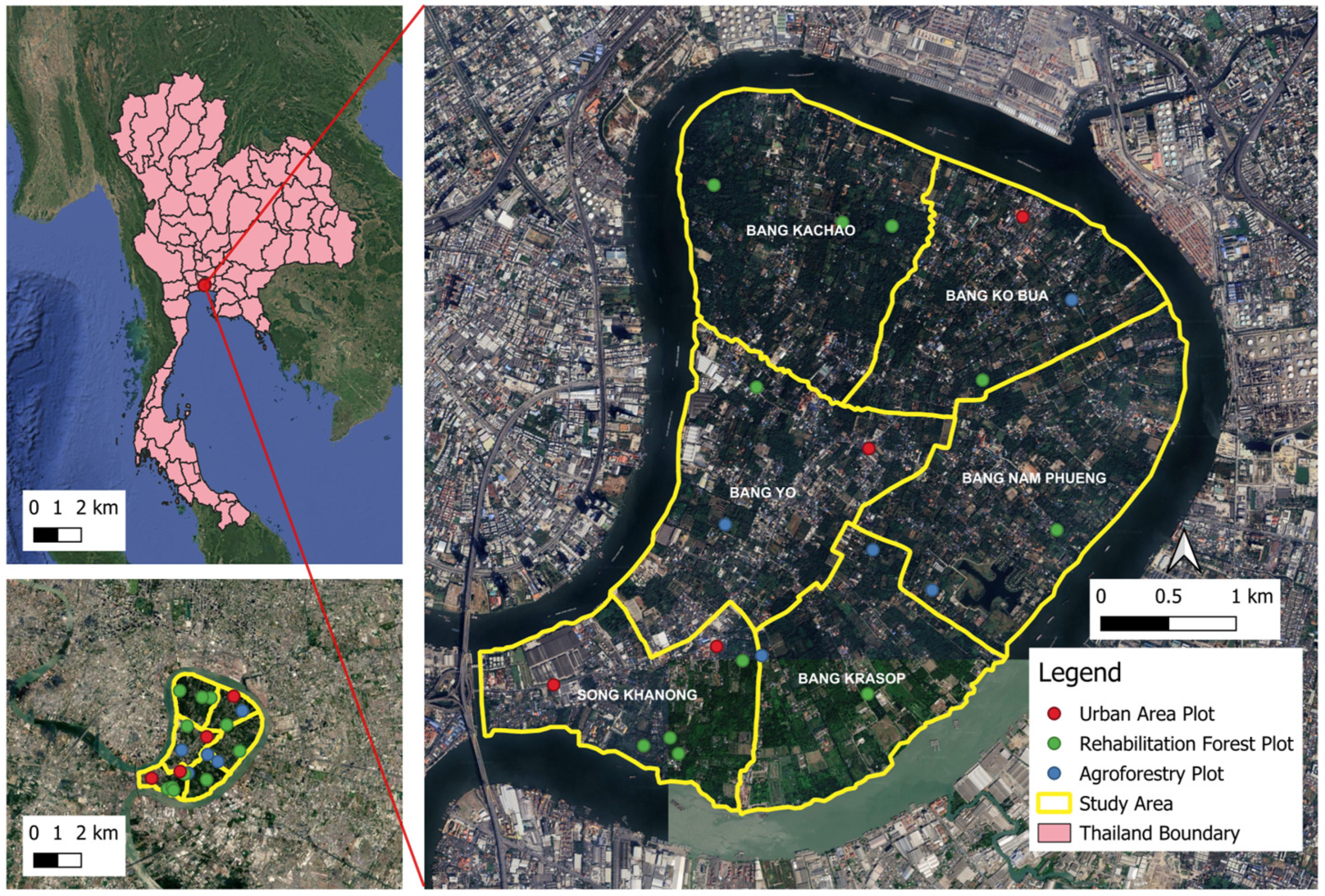
Khung Bang Kachao is an expansive riparian green space formed by a prominent oxbow meander of the Chao Phraya River, situated approximately 2 km southeast of Bangkok’s central business district within Phra Pradaeng District, Samut Prakan Province, Thailand. It represents a critically important case study for urban green space research in tropical Asia. The area covers approximately 1576.51 hectares and encompasses six subdistricts (tambons): Bang Kachao, Bang Ko Bua, Bang Nam Phueng, Bang Yo, Bang Krasop, and Song Khanong [36,38,39]. Geographically, the river meander is situated between latitudes 13°39′17″ and 13°42′12″ North and longitudes 100°32′17″ and 100°35′14″ East (Figure 1). Its distinctive curvilinear landform, locally referred to as “the pig’s stomach”, owing to its enclosed, rounded shape, has effectively insulated the peninsula from surrounding urban development pressure. Consequently, Khung Bang Kachao has been widely recognized as “Bangkok’s green lung” and was designated the “Best Urban Oasis of Asia” [36,40,41]. The area has been designated as an Environmental Protection Area by the Thai government. Its proximity to the Bangkok Metropolitan Region, combined with ongoing pressure from industrial expansion and urbanization, makes it a site of both high conservation value and urgent policy relevance.

As a natural wetland bordered on three sides by an approximately 18 km stretch of the Chao Phraya River, Khung Bang Kachao hosts a complex ecosystem comprising freshwater, saltwater, and brackish water environments and is designated as an environmental protection zone to safeguard its urban biodiversity [33,36,39].

2.2. Methods

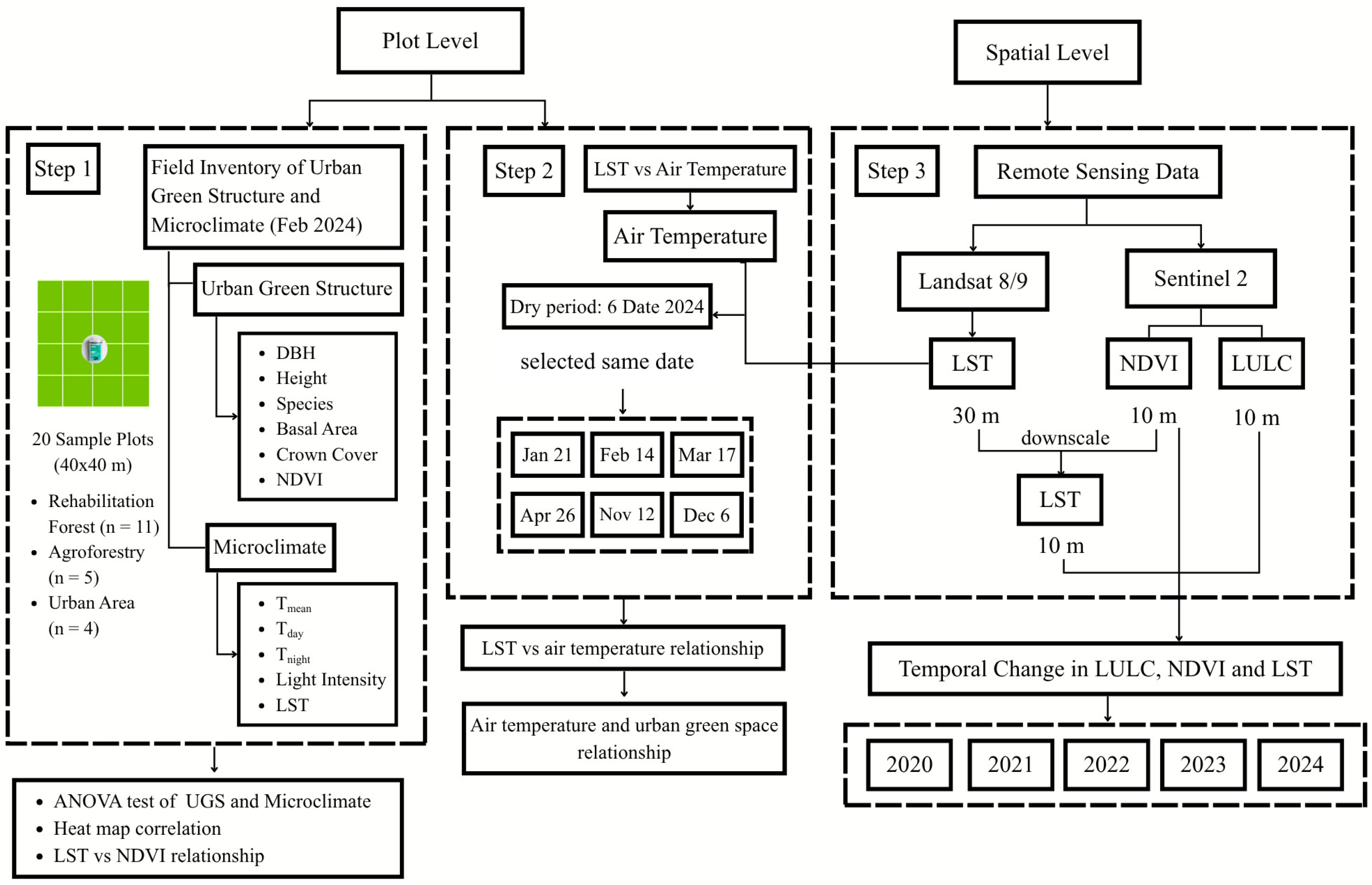
The research framework, steps, process, and methodology are shown in Figure 2. The detailed procedural steps are as follows:

2.2.1. Field Data Collection from Sample Plots of Various Urban Green Space Types

Urban Green Space Structure Survey

Field data were collected from 20 purposively selected plots (40 × 40 m; 0.16 ha per plot), distributed across three green space types: rehabilitation forest (RF: N = 11), agroforestry (AG: N = 5), and urban area (UA: N = 4). Each 40 × 40 m² plot was subdivided into sixteen 10 × 10 m² subplots for field inventory, resulting in a total of 320 subplots. Purposive sampling was applied to capture the full range of structural variation in vegetation across the study area, with plot locations selected to represent distinct land use and canopy conditions within each urban green space type. Tree species identification followed the Thai Plant Names [42]. Vegetation structure was characterized at two levels. For vertical structure, diameter at breast height (DBH) was measured for all trees with DBH ≥ 4.5 cm, total tree height was recorded, and stand basal area was calculated. For horizontal structure, Crown Cover (CC) was calculated per plot as the sum of individual tree crown projection areas, expressed as a percentage of subplot ground area. In multilayered rehabilitation forest stands, overlapping crowns at different canopy heights can therefore yield values exceeding 100%; this is an intended feature of the metric, capturing vertical canopy layering and density rather than a single bounded ground-projected cover fraction to quantify canopy density and assess its influence on solar radiation attenuation at the plot level.

Air Temperature and Light Intensity Monitoring

Air temperature and light intensity were recorded continuously using HOBO Pendant^® data loggers installed at the center of each plot at a height of 1.5 m above ground level, following standard meteorological conventions for near-surface air temperature measurement. Data were recorded at 10-min intervals throughout the year 2024, focusing on all months within the dry period (January, February, March, April, November, and December 2024), corresponding to the dry season period of maximum thermal contrast when the absence of rainfall minimizes precipitation-driven surface cooling and enhances spatial differentiation of LST signals. Recorded temperature data were aggregated into four daily metrics for each plot: daily mean air temperature, daytime mean (06:00–18:00), nighttime mean (18:01–05:59), and air temperature at the satellite overpass time (10:20–10.30 local time).

2.2.2. Satellite Data Preparation and Cloud Processing

This study analyzes multi-sensor data on the Google Earth Engine (GEE) platform using data from Sentinel-2A MSI Level-2A imagery (10-m spatial resolution), which was used to derive NDVI and Land Use/Land Cover (LULC) classifications, while Landsat 8/9 Collection 2 Level 2 thermal infrared data (TIRS/TIRS-2, 30-m resolution) were used to retrieve land surface temperature (LST) [16]. Satellite data from the dry seasons of 2020 to 2024 were selected based on a cloud cover threshold of less than 5% (Table 1). This criterion was applied to minimize atmospheric interference with thermal band retrieval and ensure the radiometric integrity of the LST estimates [15]. To systematically address the research objectives, the compiled datasets were integrated into three distinct analytical frameworks.

(1) Green Space Structure and LST Correlation (Field Plot Validation 2024).

In 2024, the extracted NDVI and LST data were temporally aligned with the field inventory period conducted within the designated sample plots. These concurrent datasets were utilized in statistical analyses to evaluate and compare the specific impacts of forest structural parameters on local LST mitigation.

(2) Long-Term Temporal Variation Analysis (2020–2024).

The broader multi-temporal composite of LULC, NDVI, and LST data spanning February from 2020 to 2024 was utilized to model, map, and analyze the 5-year temporal variations across the study area.

(3) Spatiotemporal Microclimate Coupling Analysis.

To evaluate the dynamics of the relationship between LST and in situ microclimate air temperature across green space types, an analysis was conducted on a strictly matched dataset pairing satellite-derived LST with in situ air temperature observations. This framework utilized data from six cloud-free Landsat overpass dates spanning the 2024 calendar year: 21 January, 14 February, 17 March, 26 April, 12 November, and 6 December.

2.2.3. Land Surface Temperature (LST) Calculation

Land surface temperature (LST) was retrieved from the Landsat 8/9 Collection 2 Level 2 Surface Temperature Product, which provides atmospherically corrected surface temperature values pre-processed by the United States Geological Survey [43]. Thermal radiance data were acquired via the thermal infrared sensor (TIRS) onboard Landsat 8 and the improved TIRS-2 onboard Landsat 9, the latter incorporating enhanced stray light correction to reduce thermal contamination from outside the target area and improve radiometric accuracy. LST values were extracted from Band ST_B10 by applying the Collection 2 Level 2 scale factors provided by USGS, converting raw digital numbers (DNs) to degrees Celsius using the following formula:

LST (°C) = (DN × 0.00341802 + 149.0) − 273.15

(1)

where 0.00341802 is the multiplicative scale factor, 149.0 is the additive offset, and −273.15 converts from Kelvin to degrees Celsius. This approach follows USGS-recommended preprocessing protocols for Collection 2 Level 2 products and eliminates the need for manual radiance-to-temperature conversion applied in earlier Landsat collection workflows.

Table 1. Acquisition dates and cloud cover percentages of Landsat and Sentinel satellite imagery scenes utilized for land surface temperature (LST) and Normalized Difference Vegetation Index (NDVI) analysis (2020–2024).

Landsat Imagery for LST			Sentinel Imagery for NDVI
Scene ID	Acquisition Date	Cloud Cover (%)	Scene ID	Acquisition Date	Cloud Cover (%)
LC08_129050_20200219	19 February 2020	5	20200221T033751_20200221T034107_T47PPR	21 February 2020	5
LC08_129050_20210221	21 February 2021	5	20210220T033759_20210220T035049_T47PPR	20 February 2021	5
LC08_129051_20220224	24 February 2022	5	20220101T034141_20220101T035002_T47PPR	01 February 2022	5
LC08_129050_20230227	27 February 2023	5	20230225T033721_20230225T034950_T47PPR	25 February 2023	5
LC08_129050_20240214	14 February 2024	5	20240121T034041_20240121T035215_T47PPR	21 February 2024	5

Table 1. Acquisition dates and cloud cover percentages of Landsat and Sentinel satellite imagery scenes utilized for land surface temperature (LST) and Normalized Difference Vegetation Index (NDVI) analysis (2020–2024).

Landsat Imagery for LST			Sentinel Imagery for NDVI
Scene ID	Acquisition Date	Cloud Cover (%)	Scene ID	Acquisition Date	Cloud Cover (%)
LC08_129050_20200219	19 February 2020	5	20200221T033751_20200221T034107_T47PPR	21 February 2020	5
LC08_129050_20210221	21 February 2021	5	20210220T033759_20210220T035049_T47PPR	20 February 2021	5
LC08_129051_20220224	24 February 2022	5	20220101T034141_20220101T035002_T47PPR	01 February 2022	5
LC08_129050_20230227	27 February 2023	5	20230225T033721_20230225T034950_T47PPR	25 February 2023	5
LC08_129050_20240214	14 February 2024	5	20240121T034041_20240121T035215_T47PPR	21 February 2024	5

2.2.4. Land Surface Temperature (LST) Downscale

To align LST spatial resolution with the 10-m Sentinel-2 imagery used for vegetation and land-use analysis, LST was downscaled from 30 m to 10 m within the Google Earth Engine platform using a multiple linear regression approach. The downscaling model was constructed by regressing 30 m LST values against three Sentinel-2-derived spectral indices: the Normalized Difference Vegetation Index (NDVI), the Normalized Difference Built-up Index (NDBI), and the Normalized Difference Water Index (NDWI) aggregated to the Landsat resolution. The resulting regression coefficients were then applied at 10 m resolution to produce a spatially enhanced LST surface [15]:

LST_downscaled = a + (b₁ × NDVI) + (b₂ × NDBI) + (b₃ × NDWI)

(2)

where a is the regression intercept and b₁, b₂, and b₃ are the spectral index coefficients derived from the regression within the study area. Downscaled LST values were subsequently classified into five temperature intervals (0–25, 25–30, 30–35, 35–40 and 40–100 °C) for spatial distribution analysis and temporal comparison across the 2020–2024 study period. Classification and cartographic visualization were performed in QGIS 3.38.

2.2.5. Calculation of the Normalized Difference Vegetation Index (NDVI)

The Normalized Difference Vegetation Index (NDVI) was calculated from Sentinel-2A MSI Level-2A surface reflectance data using the near-infrared (Band 8, 842 nm) and red (Band 4, 665 nm) spectral bands at 10-m spatial resolution:

NDVI = (NIR − RED)/(NIR + RED)

(3)

Sentinel-2 was selected for NDVI derivation due to its 10-m spatial resolution and 5-day revisit frequency, which provide sufficient detail for plot-level vegetation characterization in heterogeneous peri-urban landscapes [44,45]. NDVI values were classified into five vegetation density categories following established thresholds [20,46], as summarized in

Table 2. Criteria for classifying vegetation density based on the NDVI.

NDVI Value	Vegetation Density	Physical Characteristics and Structure
−1–0	Water bodies	water bodies (rivers/canals), or building shadows
0–0.2	Vegetation-free areas	buildings, roads, concrete surfaces, or vacant land
0.2–0.4	Low density	lawns, small vegetation, or widely spaced trees
0.4–0.6	Medium density	dense shrublands, parks, or mixed green spaces
>0.6	High density	areas with dense canopies (closed canopy), forested areas

. The full NDVI range from −1 to 1 was retained to preserve the spectral distinction between water bodies and shadowed surfaces (NDVI < 0), sparsely vegetated areas, and closed-canopy forest cover (NDVI > 0.6), enabling cleaner separation of surface types in the LST–vegetation relationship analysis. Values between −1 and 0 indicate surfaces with higher near-infrared absorption than red-wavelength absorption, characteristic of water bodies and shaded areas [46]. This classification allows for more accurate analysis of the NDVI–LST relationship by clearly separating the influence of water bodies from vegetation [20].

2.2.6. Land Use/Land Cover Classification (LULC)

Time-series multispectral imagery from the Sentinel-2 Level-2A dataset was processed via the Google Earth Engine (GEE) platform [16] to characterize Land Use/Land Cover (LULC) dynamics between 2020 and 2024 (Appendix A). To mitigate seasonal variations and cloud contamination, data acquisition was restricted to the January–May window of each year. A robust preprocessing protocol was applied, utilizing the Scene Classification (SCL) band to mask clouds and shadows, followed by a per-pixel median reducer to generate radiometrically consistent, cloud-free annual composites [44]. A Random Forest (RF) machine learning classifier [47] configured with 100 decision trees [48] was trained using reference data comprising ten distinct LULC typologies extracted from the 2022 baseline composite. Following a spatially stratified 80/20 train–test split for model calibration and validation, the RF algorithm was extrapolated to classify the remaining temporal composites, and the true surface area of each predicted category was subsequently quantified using the ee.Image.pixelArea() function to account for geodetic curvature [49].

A total of 149 Sentinel-2 scenes were utilized to generate the annual cloud-free median composites from 2020 to 2024. The data selection was constrained to the first five months of each year to capture distinct surface features while mitigating peak monsoon cloud cover [50].

Table 3. Summary of Sentinel-2 imagery utilized for annual LULC classification (2020–2024).

Year	Total Scenes Processed	Acquisition Period	Average Cloud Cover (%)
2020	30	02 January 2020–26 May 2020	24.50
2021	30	01 January 2021–26 May 2021	42.09
2022	30	01 January 2022–26 May 2022	48.33
2023	28	01 January 2023–26 May 2023	38.78
2024	31	01 January 2024–30 May 2024	31.62

summarizes the acquisition periods, the total number of scenes processed per year, and the average pre-masking cloud cover. By leveraging this dense stack of multispectral observations, specifically the blue, green, red, near-infrared, and shortwave infrared bands, the methodology successfully generated continuous, artifact-free spatial datasets, enabling a highly accurate and standardized longitudinal assessment of landscape transformations [51].

Classification followed the Level 1 land-cover typology of the Department of Land Development of Thailand [52], comprising five categories: (1) community and built-up areas, including settlements, commercial zones, and infrastructure; (2) agricultural areas, including cultivated and managed farmland; (3) forest areas, including natural and rehabilitated tree cover; (4) water bodies, including rivers, canals, and reservoirs; and (5) miscellaneous areas, encompassing all remaining land surface types.

2.2.7. Analysis of the Relationship Between LST and Air Temperature

To evaluate the relationship between LST and in situ microclimate air temperature across green space types while accounting for the repeated-measures structure (6 dates × 20 plots, N = 120) and resolving non-independence among within-plot observations, a linear mixed model (LMM) was fitted using restricted maximum likelihood (REML) with plot specified as a random intercept. The dataset was constructed by pairing plot-level satellite-derived LST (retrieved from six cloud-free Landsat overpasses in 2024: 21 January, 14 February, 17 March, 26 April, 12 November and 6 December (

Table 4. Acquisition dates and cloud cover percentages of paired Landsat imagery scenes utilized for LST–air temperature relationship analysis for the dry period in 2024.

Year 2024	Landsat Imagery for LST				Date of Air Temperature from HOBO Data Logger
Month of Dry Period	Scene ID	Acquisition Date	Acquisition Time	Cloud Cover (%)	Urban (4 Plots)	Rehabilitation Forest (11 Plots)	Agroforestry (5 Plots)	Observation Time
January	LC09_129051_20240121	21 January 2024	10:27	5	21 January 2024			10:20–10:30
February	LC08_129050_20240214	14 February 2024	10:27	5	14 February 2024			10:20–10:30
March	LC08_129051_20240317	17 March 2024	10:27	5	17 March 2024			10:20–10:30
April	LC09_129050_20240426	26 April 2024	10:27	5	26 April 2024			10:20–10:30
November	LC08_129051_20241112	12 November 2024	10:27	5	12 November 2024			10:20–10:30
December	LC09_129050_20241206	6 December 2024	10:27	5	6 December 2024			10:20–10:30
Total Sample (N)					120

)) with the corresponding in situ ambient air temperature recorded by HOBO data loggers at the exact satellite overpass time (10:20–10:30 local time).

Model optimization was performed using Backward Elimination, starting with a full model containing month and urban green space structure variables (Month, LST, Light Intensity, NDVI, DBH, Height, Basal Area, Species, Tree Density, and Canopy Cover). Non-significant terms (p > 0.05) were sequentially dropped until arriving at the final reduced LMM, retaining only truly significant fixed terms. Subsequently, post hoc linear regressions between actual air temperature and model-predicted values were conducted for the full dataset and stratified by green space type (rehabilitation forest, agroforestry, and urban area) to evaluate model performance across different landscape management green space types.

3. Results

3.1. Urban Green Space Structure and Air Temperature

Based on the comparative analysis of means (±SD) across 12 variables covering 7 green space structural factors (DBH, height, basal area, tree density, crown cover, number of species, and NDVI), and 5 microclimatic factors (LST, mean air temperature (T_mean), day air temperature (T_day), night air temperature (T_night), and light intensity) among three urban green space type as agroforestry (N = 5), rehabilitation forest (N = 11), and urban area (N = 4), totaling 20 sampling plots are shows in

Table 5. Comparative mean analysis with ANOVA test of urban green space structural factors (DBH, height, basal area, tree density, crown cover, number of species, and NDVI) and microclimate factors (LST, mean air temperature (T_mean), daytime air temperature (T_day), nighttime air temperature (T_night), and light intensity), among rehabilitation forest, agroforestry, and urban area in Khung Bang Kachao.

Parameter	Plot-Level ANOVA			ANOVA
	Rehabilitation Forest (N = 11)	Agroforestry (N = 5)	Urban Area (N = 4)
	Mean ± SD	Mean ± SD	Mean ± SD	F
1. Green Space Structure
DBH (cm)	12.69 ± 2.94	9.04 ± 6.23	17.33 ± 11.96	1.94ns
Height (m)	8.31 ± 1.74	4.41 ± 2.52	4.32 ± 3.19	7.59 **
Species	12.55 ± 5.05	7.40 ± 5.03	2.75 ± 1.89	7.08 **
Basal Area (m2/ha)	7.49 ± 4.85	1.56 ± 0.95	7.86 ± 13.18	1.48 ns
Tree Density (trees/ha)	535.80 ± 320.60	207.50 ± 230.12	26.56 ± 19.35	6.16 **
Crown Cover (%)	53.88 ± 50.90	14.05 ± 10.78	3.98 ± 4.48	3.20 ns
NDVI (February 2024)	0.48 ± 0.07	0.41 ± 0.05	0.18 ± 0.07	28.23 ***
2. Microclimate of February
Mean Air Temperature (°C)	29.65 ± 0.95	30.60 ± 0.39	30.90 ± 1.00	4.03 *
Daytime Air Temperature (°C)	31.69 ± 1.72	34.28 ± 0.67	33.60 ± 1.50	6.04 *
Nighttime Air Temperature (°C)	27.61 ± 0.49	26.92 ± 0.16	28.19 ± 0.56	9.08 **
Light Intensity (lux)	10,188.69 ± 12,524.73	23,473.05 ± 9903.99	15,216.50 ± 9954.06	2.29 ns
LST (°C) (February 2024)	33.86 ± 1.36	35.19 ± 1.26	40.77 ± 0.26	48.08 ***

Significance codes: ns = not significant, * = p < 0.05, ** = p < 0.01, *** = p < 0.001.

. The One-Way ANOVA test demonstrated significant statistical differences across green space types for structural traits, such as tree height (p < 0.01), number of tree species (p < 0.01), tree density (p < 0.01), and NDVI (p < 0.001), as well as all air temperature metrics and LST, reflecting that green space structures significantly influence both temperature and urban microclimate.

The results of urban green space structure showed that the NDVI reached its highest in the rehabilitation forest at 0.48 ± 0.07 (F = 28.23, p < 0.001), indicating high vegetation density and health, followed by agroforestry at 0.41 ± 0.05 and lowest in urban areas with a value of 0.18 ± 0.07. This showed a significant lack of green space in urban areas.

Tree height (Ht) peaked in the rehabilitation forest with a mean of 8.31 ± 1.74 m (F = 7.59, p < 0.01), signifying a mature forest stand. In contrast, agroforestry at 4.41 ± 2.52 m and the urban area at 4.32 ± 3.19 m displayed similar mean values. However, the standard deviation (SD) was higher in the urban area, showing a wider variation in urban tree heights.

Number of tree species (SP.) was highest in the rehabilitation forest, averaging 12.55 ± 5.05 species (F = 7.08, p < 0.01), followed by agroforestry with 7.40 ± 5.03 species, and lowest in the urban area with 2.75 ± 1.89 species. Tree density (F = 6.16, p < 0.01) was significantly higher in the rehabilitation forest (535.80 ± 320.60 trees/ha), followed by agroforestry (207.50 ± 230.12 trees/ha), and lowest in the urban area (26.56 ± 19.35 trees/ha).

Crown cover percentage (CC) was highest in the rehabilitation forest, averaging 53.88 ± 50.90% (F = 3.20, p > 0.05), resulting from multilayered canopy overlap. In contrast, crown cover of agroforestry was 14.05 ± 10.78%, and the urban area hit the lowest point at 3.98 ± 4.48%, highlighting a large lack of tree canopy cover in urban environments.

Diameter at breast height (DBH) reached its highest average in the urban area at 17.33 ± 11.96 cm (F = 1.94, p > 0.05), which can be attributed to the fact that urban trees are primarily planted individually, offering ample growth space, and are often mature in age. Rehabilitation forest presented an intermediate mean value of 12.69 ± 2.94 cm, while agroforestry exhibited the lowest value at 9.04 ± 6.23 cm due to high-density planting and active pruning management.

Basal area (BA) was largest in the urban area with a mean of 7.86 ± 13.18 m²/ha (F = 1.48, p > 0.05), followed closely by rehabilitation forest at 7.49 ± 4.85 m²/ha. Urban area demonstrated a high standard deviation of 13.18, indicating high structural variability among urban trees. Agroforestry yielded the minimum value at 1.56 ± 0.95 m²/ha due to smaller tree sizes and wider planting intervals.

For daytime air temperature (T_day) (F = 6.04, p < 0.05), agroforestry had the highest Tday of 34.28 ± 0.67 °C, exceeding the urban area at 33.60 ± 1.50 °C. The open canopy in agroforestry areas allows more direct sunlight, leading to higher daytime temperatures. On the other hand, the rehabilitation forest recorded the lowest daytime temperature of 31.69 ± 1.72 °C due to dense canopy shading.

Nighttime air temperature (T_night) (F = 9.08, p < 0.01) peaked in the urban area with a mean of 28.19 ± 0.56 °C, due to heat release from concrete and asphalt surfaces. Conversely, agroforestry had the lowest nighttime temperature of 26.92 ± 0.16 °C, while rehabilitation forest showed an intermediate value of 27.61 ± 0.49 °C.

Mean air temperature (T_mean) (F = 4.03, p < 0.05) showed that the urban area recorded the highest daily mean of 30.90 ± 1.00 °C, followed by agroforestry at 30.60 ± 0.39 °C, and rehabilitation forest at 29.65 ± 0.95 °C. Although the overall difference is small (~1.25 °C), it remains statistically significant due to the low variance within each green space type.

Light intensity (F = 2.29, p > 0.05) was highest in agroforestry, with an average of 23,473.05 ± 9903.99 lux due to its open canopy. The rehabilitation forest had the lowest light levels at 10,188.69 ± 12,524.73 lux because the dense tree cover blocks sunlight. The urban area recorded a middle value of 15,216.50 ± 9954.06 lux with a high SD, due to the fragmented distribution of city trees.

These structural differences among urban green space types directly influenced thermal dynamics and microclimates. The findings indicate that LST (F = 48.08, p < 0.001) serves as the most distinct differentiator among urban green space types, yielding the highest F-value across all parameters. The urban area registered the highest mean land surface temperature of 40.77 ± 0.26 °C, whereas rehabilitation forest achieved the lowest land surface temperature of 33.86 ± 1.36 °C, and agroforestry occupied an intermediate position at 35.19 ± 1.26 °C. The temperature gap of up to 6.91 °C between the urban area and the rehabilitation forest clearly demonstrates the urban heat island effect, highlighting the high efficiency of rehabilitation forests in mitigating land surface temperatures.

3.2. Correlation Between Green Space Structure and Temperature (LST and Air Temp.)

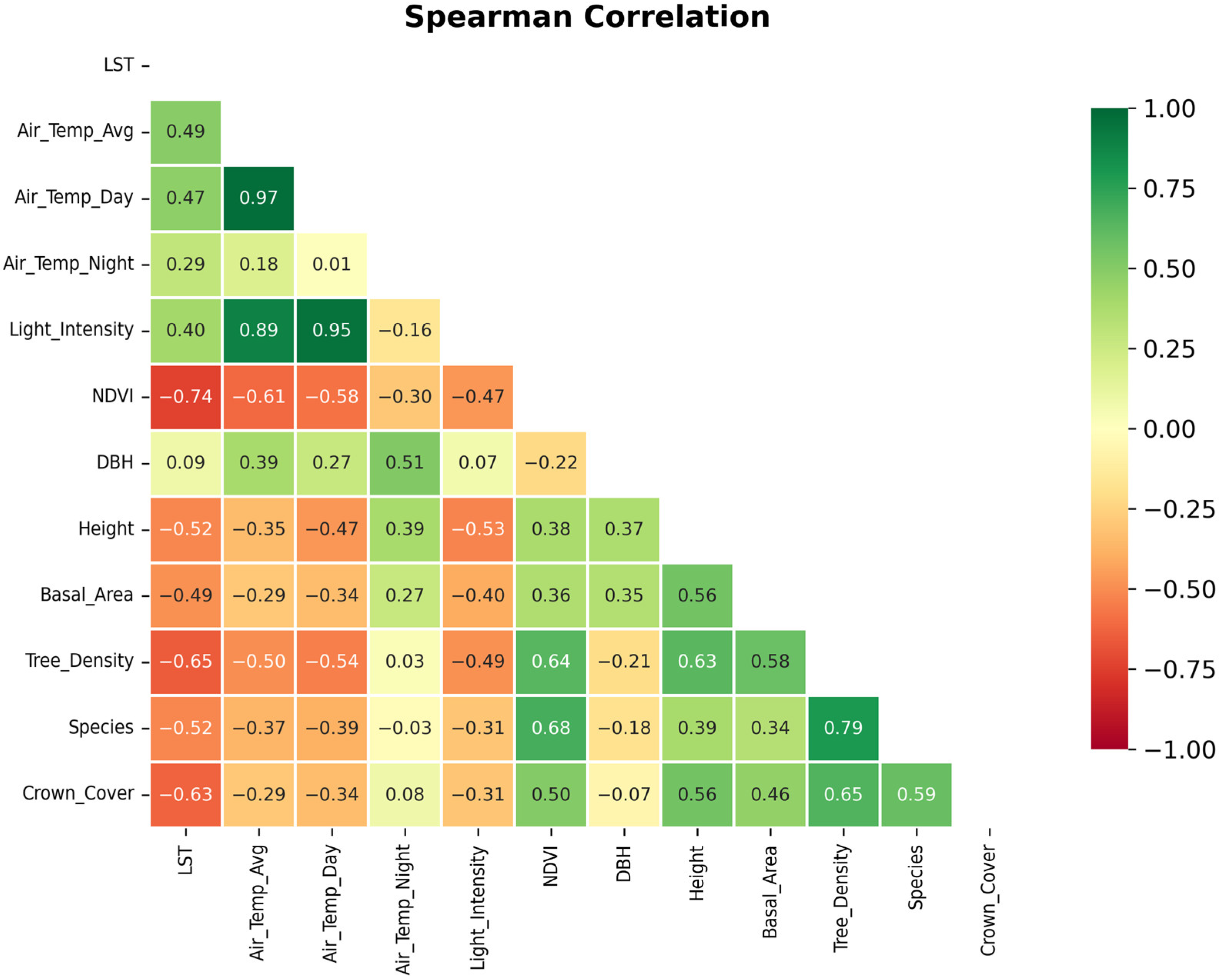
Spearman’s rank correlation analysis revealed significant negative associations between LST and all vegetation structural attributes. NDVI exhibited the strongest inverse relationship with LST (r = −0.74), followed by tree density (r = −0.65), crown cover (r = −0.63), species richness (r = −0.52), tree height (r = −0.52), and basal area (r = −0.49). These results indicate that plots with denser, taller, and more species-rich canopies consistently recorded lower surface temperatures, confirming that vegetation structural complexity contributes independently to LST mitigation beyond what greenness indices alone capture (Figure 3). Furthermore, urban green structural attributes demonstrated significant negative associations with air temperatures. NDVI exhibited the strongest inverse relationships with both average air temperature (r = −0.61) and daytime air temperature (r = −0.58), followed closely by tree density (r = −0.50 and r = −0.54, respectively). Conversely, a distinct microclimatic pattern emerged at night, where nighttime air temperature displayed unexpected positive correlations with DBH (r = 0.51) and tree height (r = 0.39), reflecting the heat-trapping dynamics associated with isolated large trees within the urban environment.

Strong positive intercorrelations were observed among structural attributes, particularly between species richness and tree density (r = 0.79), tree density and crown cover (r = 0.65), and NDVI and tree density (r = 0.64). These relationships reflect the co-occurrence of structural complexity in well-developed stands; plots with high stem density tend to also exhibit greater species diversity and more continuous canopy closure.

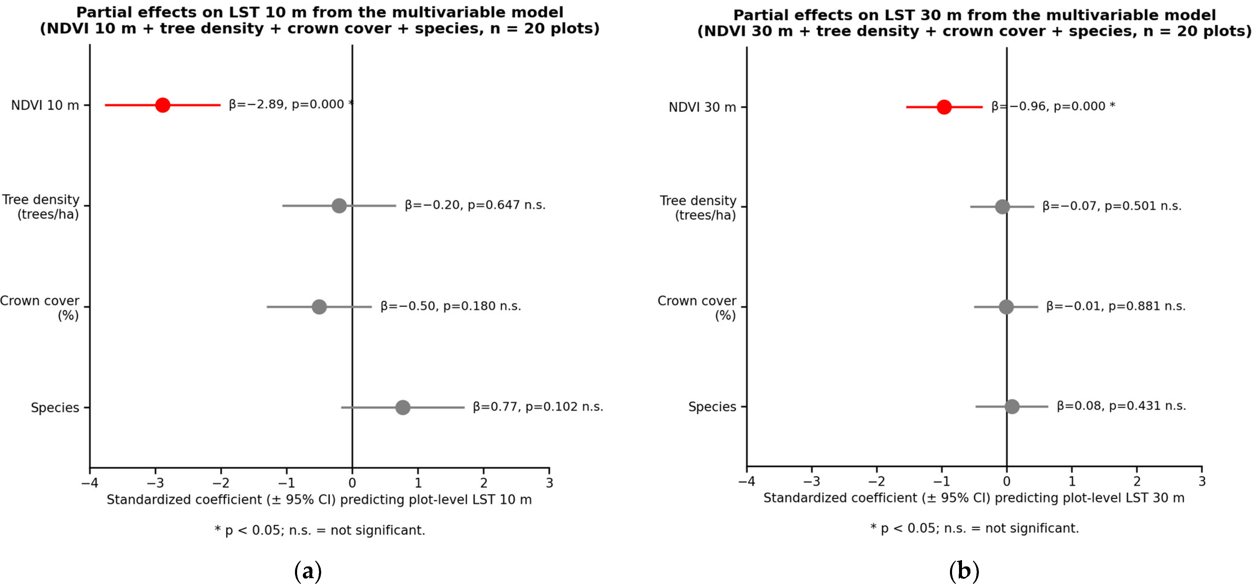
Figure 4 presents coefficient plots illustrating the partial effects of four predictor variables on plot-level LST derived from multivariable models (N = 20) across two spatial resolutions: downscaled LST 10 m and native LST 30 m. The analysis reveals that NDVI is the sole statistically significant driver of LST reduction at both plot level (β = −2.89, p < 0.001 for 10 m; β = −0.96, p < 0.001 for 30 m), with 95% confidence intervals strictly below the zero-effect threshold. In contrast, when controlling for NDVI, structural attributes and compositional diversity, namely tree density, crown cover, and species, do not exhibit statistically significant effects on LST at either resolution, as their respective confidence intervals intersect zero (p > 0.05). Consequently, within this multivariable model, overall vegetation vigor and greenness (captured by NDVI) serve as the primary explanatory factor mitigating plot-level thermal dynamics, whereas localized variations in structural density, canopy cover, and species provide no additional statistically significant explanatory power.

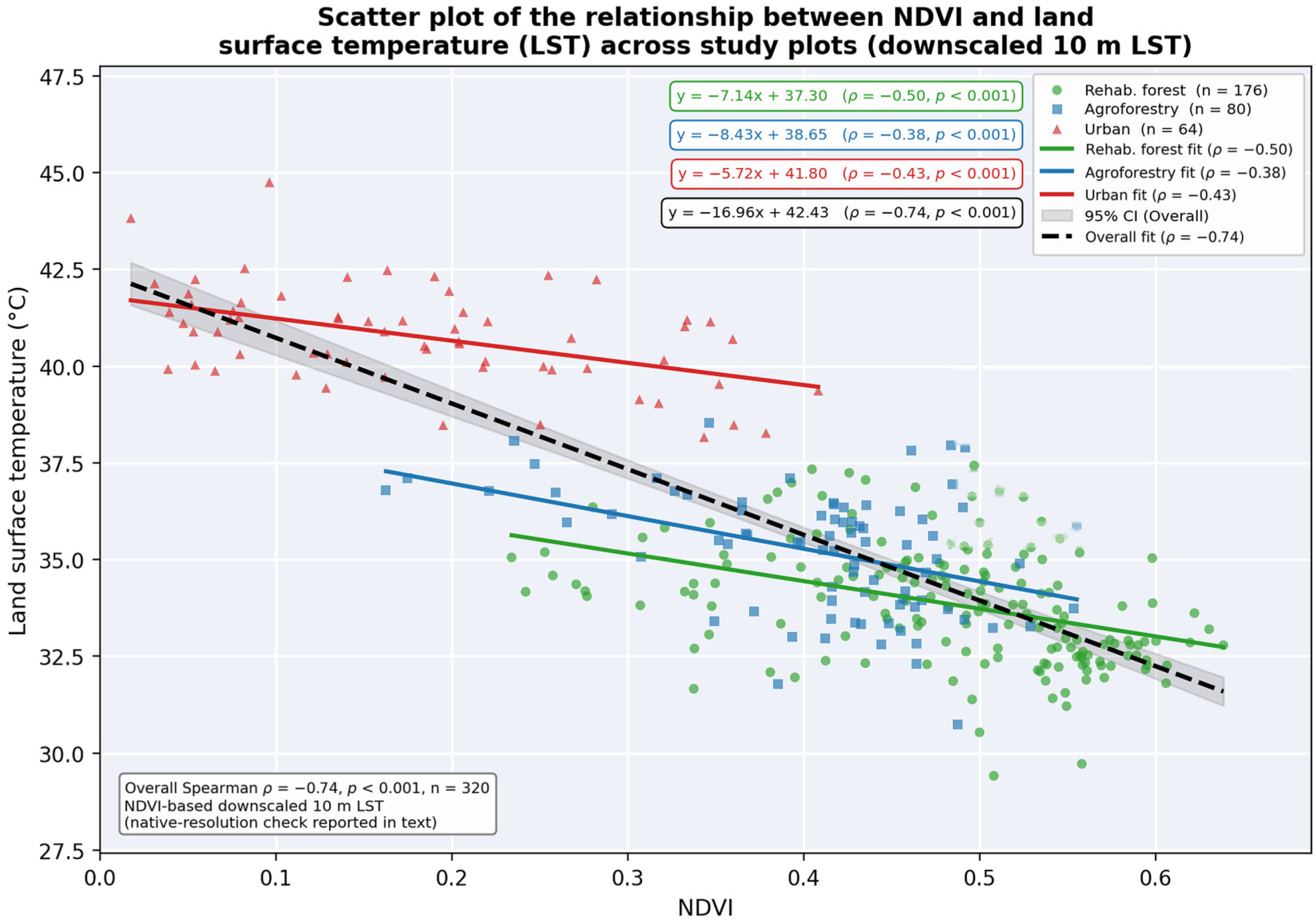
At the spatial level, bivariate analysis of the NDVI–LST relationship using the downscaled 10 m LST product revealed a strong negative correlation across all plots (Spearman’s ρ = −0.74, p < 0.001, N = 320; Figure 5). Because NDVI was one of three predictors (alongside NDBI and NDWI) used to statistically downscale the 30 m Landsat LST to 10 m resolution, this correlation is expected to be inflated relative to any intrinsic, native-resolution NDVI–LST relationship and should be interpreted as a property of the downscaling model rather than as independent evidence of NDVI’s thermal-regulating role.

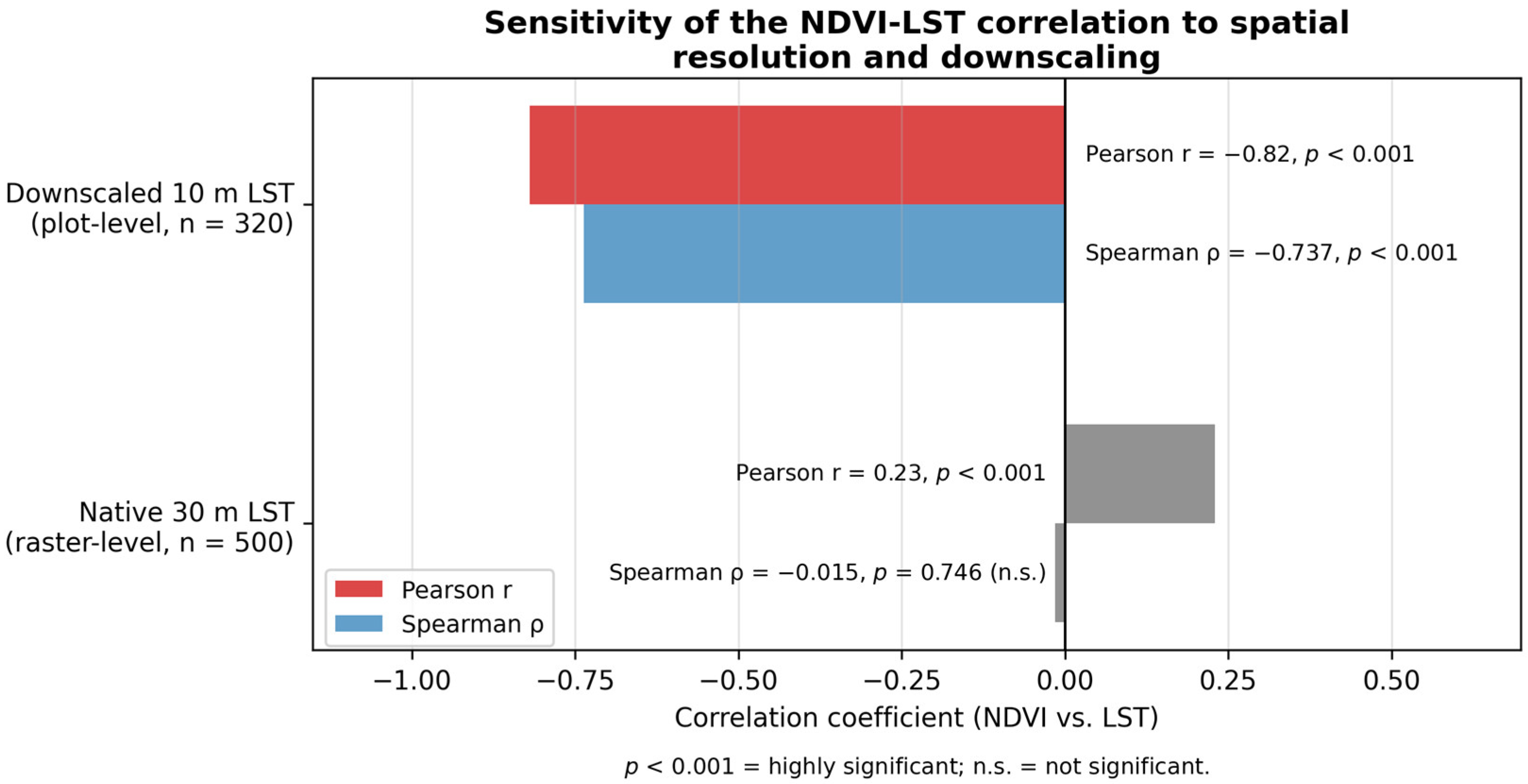
To evaluate this independently, we correlated NDVI against the native 30 m Landsat LST, before any downscaling, using 500 randomly sampled points across the study area. This native-resolution check showed a markedly weaker relationship: Pearson’s r = 0.235 (p < 0.001), notably positive rather than negative, and no significant monotonic relationship by Spearman’s ρ (ρ = −0.015, p = 0.746) (Figure 6). This indicates that NDVI alone is a weak and inconsistent predictor of LST at native resolution, and that the strong negative pattern observed after downscaling (Figure 5) substantially reflects the combined, multivariate structure of the downscaling regression (R² = 0.675, RMSE = 2.01 °C) in which NDBI and NDWI jointly contribute the built-up and moisture or water signal rather than a standalone NDVI cooling effect.

Urban green space type in the downscaled data remains informative for describing spatial thermal contrast, even under this caveat. Urban area plots recorded the lowest NDVI (predominantly < 0.4) and highest LST (38–44 °C), with the shallowest slope (−5.72 °C per unit NDVI), consistent with the persistent thermal effect of impervious surfaces largely decoupled from vegetation greenness. Agroforestry plots occupied an intermediate position (NDVI ≈ 0.3–0.5, LST 32–38 °C). Rehabilitation forest plots recorded the highest NDVI (up to 0.6+) and lowest LST, with several plots below 30 °C. In the NDVI overlap zone (0.3–0.5), rehabilitation forest plots recorded marginally lower LST than agroforestry plots at equivalent NDVI, suggesting that even at the same NDVI level, additional canopy features, such as crown continuity and vertical stratification, help explain why rehabilitation forest plots remain cooler than agroforestry plots. The maximum LST difference between low NDVI urban area plots and high NDVI rehabilitation forest plots reached 10–14 °C.

We emphasize that these urban green space type comparisons describe spatial LST patterns associated with land-cover class and should not be read as validating NDVI as an independent, native resolution driver of LST; the native resolution check (Figure 6) indicates that the relationship is weak to non-existent outside of the downscaling model’s multivariate structure.

3.3. Land Use/Land Cover and Temporal Dynamics Change in NDVI and LST (2020–2024)

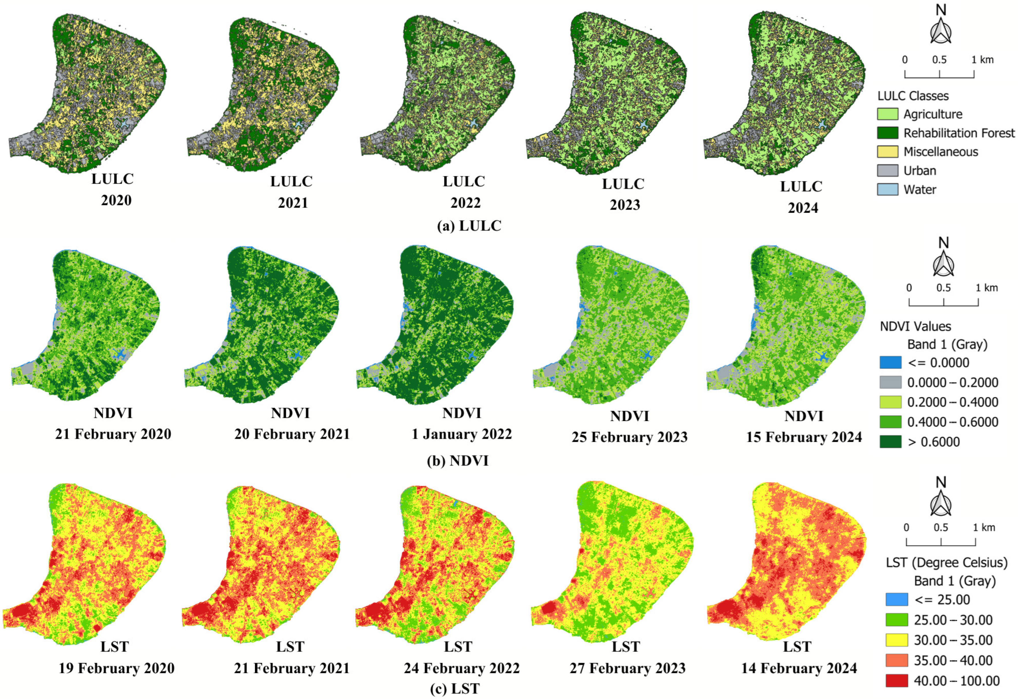
The convergence of LULC, NDVI, and LST trends across the five years points to a coherent land degradation trajectory in the Khung Bang Kachao enclave. Rehabilitation forest conversion to agricultural land between 2021 and 2024 reduced the extent of closed canopy cover, diminished evapotranspiration capacity, and increased the proportion of low-albedo, high heat absorption surfaces, collectively driving the thermal intensification recorded in 2024. The loss of tall tree canopy specifically removes the shading and latent heat exchange mechanisms identified in the plot-level analysis as the primary structural drivers of LST reduction. The 2024 thermal conditions, with nearly half the study area exceeding 35 °C, represent a significant departure from the cooler baseline recorded in 2023 and underscore the thermal consequences of continued forest loss within a designated environmental protection zone (Figure 7).

This is a result of the land-use changes that have occurred. Khung Bang Kachao rehabilitation forest, which was predominantly forested in 2021 (31.94%), has become agricultural land in 2024 (45.94%). The rehabilitation forest area has continuously decreased from 503.54 hectares to only 189.42 hectares. The Normalized Difference Vegetation Index (NDVI) response correlates with land-use change (LULC). 2022 saw the densest and most abundant vegetation (NDVI > 0.6 in 59.19%), but from 2023–2024, vegetation density decreased sharply, with most areas shifting to an NDVI range of 0.2–0.6. This impacted the change in surface temperature (LST Trend), most notably in 2024, the hottest year on record, with almost half the area (48.55%) experiencing temperatures of 35–40 °C, a significant increase from the cooler year of 2023. This increase in surface temperature coincides with the conversion of rehabilitation forests to agriculture and urban areas. The loss of shade and transpiration from large trees allows the area to accumulate more heat.

Dense vegetation cover (NDVI > 0.6) increased progressively from 19.64% in 2020 to a five-year peak of 59.19% in 2022, indicating active vegetation recovery during this period. This trend reversed sharply in 2023, when the high-density class collapsed to 1.55%, with the majority of the study area shifting to moderate NDVI classes (0.2–0.6). By 2024, only 2.98% of the study area retained high-density vegetation cover (NDVI > 0.6), while moderate density classes (0.2–0.4 at 35.60% and 0.4–0.6 at 42.28%) together accounted for 77.88% of the area. The abrupt decline between 2022 and 2023 corresponds closely to the large-scale agricultural expansion recorded in the LULC data during the same interval, suggesting that land conversion was the primary driver of vegetation density loss (

Table 6. Land Use/Land Cover Change Data, 2020–2024 (Hectares).

LULC/ Year	Rehabilitation Forest		Agricultural		Miscellaneous		Urban		Water		Total		Overall Accuracy (%)	Kappa Coefficient
	Area (ha)	%	Area (ha)	%	Area (ha)	%	Area (ha)	%	Area (ha)	%	Area (ha)	%
2020	338.40	21.47	231.23	14.67	599.75	38.04	402.68	25.54	4.45	0.28	1576.51	100	77.60	0.71
2021	503.54	31.94	142.14	9.02	616.61	39.11	309.76	19.65	4.46	0.28	1576.51	100	88.80	0.86
2022	284.85	18.07	672.80	42.68	354.08	22.46	257.73	16.35	7.05	0.45	1576.51	100	93.20	0.91
2023	257.10	16.31	728.99	46.24	327.55	20.78	256.68	16.28	6.19	0.39	1576.51	100	92.90	0.91
2024	189.42	12.02	724.30	45.94	353.84	22.44	302.38	19.18	6.57	0.42	1576.51	100	93.10	0.91

,

Table 7. Normalized Difference Vegetation Index (NDVI) Classification Data, 2020–2024 (Hectares).

NDVI Value	>−1		0–0.2		0.2–0.4		0.4–0.6		0.6–1.0		Total
	Area (ha)	%	Area (ha)	%	Area (ha)	%	Area (ha)	%	Area (ha)	%	Area (ha)	%
2020	22.60	1.43	162.68	10.32	395.56	25.09	686.04	43.52	309.64	19.64	1576.51	100
2021	29.07	1.84	126.40	8.02	273.45	17.35	412.70	26.18	734.90	46.62	1576.51	100
2022	27.44	1.74	107.44	6.82	205.68	13.05	302.87	19.21	933.08	59.19	1576.51	100
2023	30.17	1.91	250.44	15.89	503.43	31.93	768.01	48.72	24.46	1.55	1576.51	100
2024	25.36	1.61	276.35	17.53	561.20	35.60	666.55	42.28	47.05	2.98	1576.51	100

and

Table 8. Land Surface Temperature (LST) Classification Data, 2020–2024 (Hectares).

LST (°C)	<25		25–30		30–35		35–40		>40		Total
	Area (ha)	%	Area (ha)	%	Area (ha)	%	Area (ha)	%	Area (ha)	%	Area (ha)	%
2020	7.33	0.46	184.02	11.67	719.85	45.66	540.06	34.26	125.25	7.94	1576.51	100
2021	5.05	0.32	89.44	5.67	669.85	42.49	594.49	37.71	217.67	13.81	1576.51	100
2022	10.48	0.66	270.44	17.15	667.94	42.37	421.13	26.71	206.52	13.10	1576.51	100
2023	2.95	0.19	508.11	32.23	836.32	53.05	207.35	13.15	21.77	1.38	1576.51	100
2024	0.00	0.00	11.96	0.76	644.25	40.87	765.44	48.55	154.84	9.82	1576.51	100

cover annual LULC class areas, NDVI class areas, and LST class areas. In summary, 2024 was the hottest year in the five-year record, with nearly 50% of the study area falling in the 35–40 °C LST class and only 0.76% remaining below 30 °C. Over the same period, rehabilitated forest cover declined from 31.94% (2021) to 12.02% (2024), while agricultural area expanded from 9.02% to 45.94%, and dense vegetation cover (NDVI > 0.6) collapsed from 59.19% (2022) to 2.98% (2024).

Overall accuracy assessment across the 2020–2024 period demonstrated strong and consistently improving classification performance for the Khung Bang Kachao land-cover maps. Overall accuracy rose from 77.60% in 2020 to a peak of 93.20% in 2022, with corresponding Kappa coefficients spanning 0.71 to 0.91. Classification accuracy exhibited a rapid improvement from 2020 to 2022, followed by a stable plateau through 2023 (92.90%, Kappa = 0.91) and 2024 (93.10%, Kappa = 0.91). Agreement was classified as substantial only in 2020 (Kappa = 0.61–0.80), improving to almost perfect from 2021 onward (Kappa > 0.80). These results indicate that the Random Forest classifier implemented in Google Earth Engine performed reliably and with increasing consistency over time, with the comparatively lower accuracy in 2020 likely attributable to a smaller and less representative reference sample size in the earliest year of monitoring (see Appendix B).

For Land Use/Land Cover (LULC) changes between 2020 and 2024, in 2020–2021, agricultural land was only about 9–14%, but in 2022, it surged to 42.87% and remained stable at around 45–46% in 2024. In contrast, forest area peaked in 2021 at 31.94% but then continuously decreased to only 12.02% in 2024. This means that almost two-thirds of the rehabilitation forest area disappeared within three years and was changed to primarily agricultural land (Table 6).

In addition to this change in rehabilitation forest area, it was also found that miscellaneous land decreased by almost half in 2022 (from 38.04% to 22.46%), which corresponds to the increase in agricultural land. This is likely due to the conversion of miscellaneous land into agricultural land. Other areas, such as urban areas, showed a declining trend during 2020–2023 before increasing in 2024 to 19.18%, while water bodies accounted for a very small and relatively stable proportion (0.28–0.42%).

Analysis of data from three factors of LULC, NDVI, and LST during the period between 2020 and 2024 revealed that severe land transformation occurred in the Khung Bang Kachao area over the past five years. This was due to rapid agricultural expansion, which directly impacted NDVI and LST.

Showing the changes in the NDVI between 2020 and 2024 reveals an increasing trend in the NDVI in the Khung Bang Kachao area during 2020–2022, particularly in the NDVI range of 0.6–1.0 (which represents very dense green areas or rehabilitation forest). It was found that the percentage of rehabilitation forest area in this NDVI group increased from 19.64% in 2020 to a high of 59.19% in 2022. This suggests that Khung Bang Kachao experienced substantial forest restoration and a high density of green coverage between 2020 and 2022 (Table 7).

However, subsequently, a significant fluctuation in NDVI was observed in 2023. The proportion of dense vegetation (NDVI 0.6–1.0) experienced a sharp decline from 59.19% to 1.55%. Concurrently, nearly 80% of the vegetative area shifted into the moderate range (NDVI 0.2–0.6), indicating a substantial reduction in both canopy density and overall vegetative health across Khung Bang Kachao. In 2024, the majority of the area was in the NDVI group (0.4–0.6), which accounted for 42.28%, and NDVI (0.2–0.4). This accounts for 35.60%, which is medium- to low-density green space, leaving only about 3% with rehabilitation forest area (NDVI greater than 0.6).

Green space cover peaked in 2021 at 503.54 hectares (31.94%) before declining continuously to 189.42 hectares (12.02%) in 2024, a loss of approximately 314 hectares, representing 62.3% of the 2021 forest extent within three years. Agricultural land expanded correspondingly, from 142.14 hectares (9.02%) in 2021 to 724.30 hectares (45.94%) in 2024. Miscellaneous land comprising vacant and undeveloped areas declined from approximately 38–39% in 2020–2021 to 22.44% in 2024, suggesting conversion of previously undeveloped land to agricultural use. Urban areas showed a modest decline between 2020 and 2023 before recovering to 19.18% in 2024. Water bodies remained stable throughout the study period (0.28–0.42%) (Table 6).

Between 2020 and 2022, LST distribution remained relatively stable, with approximately 42–45% of the study area recording temperatures in the 30–35 °C range. The proportion of extreme heat (>40 °C) increased to approximately 13.10–13.81% in 2021 and 2022, indicating localized heat accumulation during this period. In 2023, a distinct cooling shift was observed: the low LST class (25–30 °C) expanded to 32.23% of the study area, up from 5–17% in preceding years, while extreme heat zones contracted to 1.38%. This cooling is consistent with the high dense vegetation cover recorded in 2022 (NDVI > 0.6 in 59.19% of the area), which likely enhanced evapotranspiration and canopy shading in the following year.

By contrast, 2024 was the warmest year in the five-year record. The 35–40 °C LST class expanded to 48.55% of the study area, extreme heat zones (>40 °C) rebounded to 9.82%, and areas below 30 °C nearly disappeared (0.76%). This thermal intensification coincides with accelerated forest loss and agricultural expansion documented in the LULC data (Table 6).

Table 8, showing the classification of land surface temperature (LST) within the Khung Bang Kachao area from 2020 to 2024, reveals significant thermal shifts. Between 2020 and 2022, temperatures remained relatively stable before beginning an upward trend, with the majority of the area (approximately 42–45%) clustering within the 30–35 °C range. During 2021 and 2022, the proportion of extreme heat zones (>40 °C) increased to approximately 13%, indicating intensified localized heat accumulation.

In contrast, 2023 marked a distinct cooling phase. Areas within the low LST range (25–30 °C) expanded significantly to 32.23%, up from the 5–17% observed in previous years. Furthermore, extreme heat zones (>40 °C) contracted to just 1.38%. This cooling trend correlates with 2022 data showing that high-density green space accounted for nearly 59.19% of the area; this dense vegetation likely facilitated temperature reduction in 2023 through enhanced evapotranspiration and canopy shading.

However, 2024 emerged as the warmest year of the five years, characterized by a sharp surge in temperatures. Nearly 50% of the study area shifted from the 30–35 °C bracket into the 35–40 °C range (48.55%). The proportion of extreme heat zones (>40 °C) rebounded to nearly 10% (9.82%), while low-temperature areas (<30 °C) nearly vanished, falling below 1% (0.76%).

3.4. Relationship Between Air Temperature and Green Space Structure

To analyze the factors influencing air temperature, a linear mixed model (LMM) was fitted with random intercepts for each sampling plot. Using nine initial predictor variables, the full model was statistically significant overall. Air temperature was significantly affected by season, specifically March (β = 2.26, p = 0.015) and April (β = 3.50, p = 0.001) compared to the baseline month of November, as well as Light Intensity (β = 1.80, p = 0.003) and Tree Height (β = 2.51, p = 0.039). In contrast, the other predictors (LST, NDVI, DBH, Basal Area, Species, Tree Density, and Crown Cover) were not statistically significant (p > 0.05) (

Table 9. Linear mixed model (LMM) analysis of the relationship between air temperature in the dry period and factors of microclimate and urban green space structure in Khung Bang Kachao.

Term	Coef.	SE	z	p-Value	95% CI Low	95% CI High	Sig.
Intercept	33.1531	1.0425	31.8014	<0.0001	31.1098	35.1963	***
C(Month) [T.December]	1.3888	1.9806	0.7012	0.4832	−2.4931	5.2708	ns
C(Month) [T.January]	0.9372	1.1614	0.8070	0.4197	−1.3391	3.2136	ns
C(Month) [T.February]	0.9317	1.0566	0.8817	0.3779	−1.1393	3.0026	ns
C(Month) [T.March]	2.2627	0.9270	2.4407	0.0147	0.4457	4.0796	*
C(Month) [T.April]	3.4952	1.0925	3.1993	0.0014	1.3540	5.6365	**
LST_z	0.9375	0.6466	1.4500	0.1471	−0.3298	2.2048	ns
Light_z	1.7997	0.6097	2.9519	0.0032	0.6048	2.9946	**
NDVI_z	−1.8742	1.1295	−1.6593	0.0971	−4.0880	0.3396	ns
DBH_z	−1.7698	1.2114	−1.4610	0.1440	−4.1441	0.6044	ns
Height_z	2.5150	1.2186	2.0638	0.0390	0.1265	4.9035	*
BasalArea_z	−0.5236	0.7531	−0.6952	0.4869	−1.9996	0.9525	ns
Species_z	0.4190	1.0020	0.4182	0.6758	−1.5449	2.3828	ns
TreeDensity_z	−1.1845	1.2779	−0.9269	0.3540	−3.6891	1.3201	ns
CrownCover_z	0.2742	0.7093	0.3865	0.6991	−1.1160	1.6643	ns
Group Var	0.6157	0.3532	1.7431	0.0813	−0.0766	1.3079	ns

Significance codes: ns = not significant, * = p < 0.05, ** = p < 0.01, *** = p < 0.001.

).

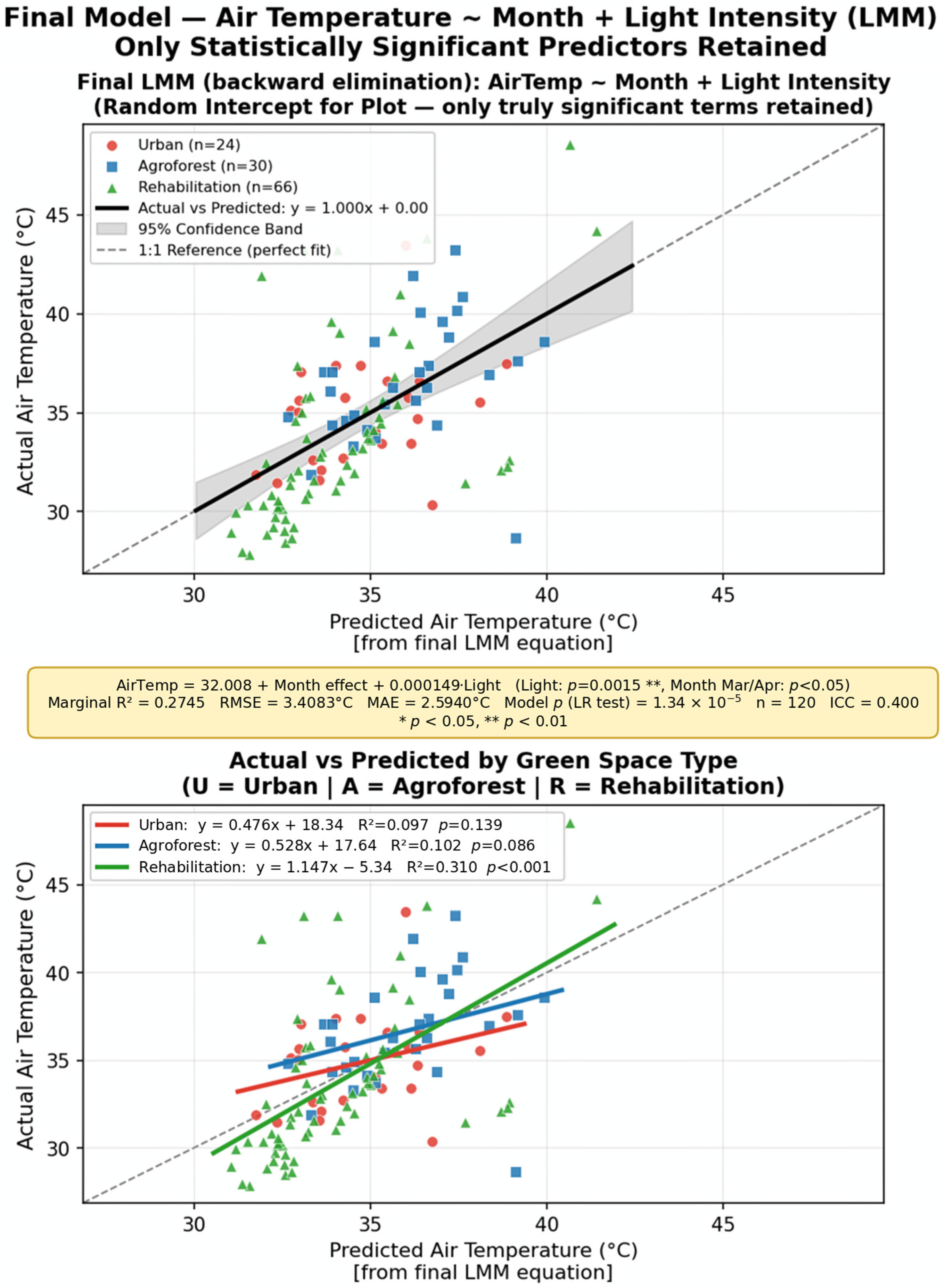
Variable selection using backward elimination was performed by removing non-significant variables step by step based on their p-values. Eight variables were removed in total: Crown Cover (p = 0.699), Species (p = 0.633), Tree Density (p = 0.437), DBH (p = 0.192), LST (p = 0.162), Tree Height (p = 0.106), NDVI (p = 0.123), and Basal Area (p = 0.153). Interestingly, LST and Tree Height lost their significance as other related vegetation variables were removed, suggesting that their initial significance was due to multicollinearity rather than a true independent effect. The final model included only Month and Light Intensity: Air Temperature = 32.008 + Month effect + 0.000149 × Light Intensity. In this final model, Light Intensity remained highly significant (p = 0.0015), along with March (p = 0.042) and April (p = 0.0037). The final model produced a Marginal R² of 0.275, Conditional R² of 0.564, RMSE of 3.4 °C, MAE of 2.5 °C, ICC of 0.40, and overall statistical significance (p = 1.34 × 10⁻⁵). Compared to the full model, this simpler model achieved better prediction accuracy with lower error values while using far fewer variables.

Finally, the relationship between air temperature in the dry period and the urban green space structure (Figure 8) showed clear differences across land types. Rehabilitation forest (N = 66) showed a significant positive relationship (slope = 1.147, R² = 0.310, p < 0.001). Agroforestry (N = 30) showed a positive trend (slope = 0.528, R² = 0.102, p = 0.086) but was not statistically significant. Urban area (N = 24) showed almost no relationship (slope = 0.476, R² = 0.097, p = 0.139). The results show that Light Intensity mainly affects air temperature in areas with dense vegetation but does not explain temperature variation in urban areas. This suggests that other unmeasured urban factors, such as surface materials, building density, or airflow, play a major role in urban areas and should be included in future models.

4. Discussion

Rapid urbanization has exacerbated the urban heat island (UHI) phenomenon in major Southeast Asian cities, necessitating effective nature-based solutions. This study evaluates the heat mitigation potential of the diverse green spaces in Thailand’s Bang Kachao curve by integrating Google Earth Engine-based remote sensing, field vegetation surveys, and microclimate monitoring across 20 experimental plots. Land surface temperature (LST) data derived from Landsat 8/9 satellites were downscaled to a 10 m resolution using Sentinel-2 spectral indices across three land-use types: rehabilitation forest, agroforestry, and urban areas.

The results indicate that green space structures significantly influence heat mitigation. Rehabilitation forest demonstrated the highest cooling capacity, maintaining an average land surface temperature 6.91 °C lower than urban areas. This finding reinforces the consensus that built-up density drives surging surface temperatures. For example, in Buriram Province, Thailand, subdistricts with 75.62% built-up density experienced temperatures 4.48 °C higher than rehabilitation forest and agricultural areas [53]. Similarly, in Southeast Asian capitals like Bangkok, Jakarta, and Manila, built-up areas average 3 °C warmer than green spaces [54], a thermal gap that widens to 4 °C in dense high-rise or industrial zones, as evidenced in Indonesia [55].

LST exhibited a statistically significant negative correlation with various forest structural parameters, most notably NDVI, tree density, canopy size, tree height, and tree species diversity (Figure 3). This inverse LST–NDVI relationship mirrors prior research in Thailand, where droughts or vegetation decline (low NDVI) trigger immediate LST increases across all seasons and regions [56,57]. Consistently, studies in tropical and temperate urban areas, such as those in Thailand, Indonesia, the Philippines, Bangladesh, India, and South Korea, confirm that high NDVI values and extensive forest patches enhance cooling capacities to mitigate urban heat islands [54,58,59]. Regarding tree density, the findings in Khung Bang Kachao corroborate regional evidence from Southeast Asia and South Korea, demonstrating that denser vegetation within small green spaces effectively keeps internal forest LST lower than surrounding built-up environments [54,58]. Furthermore, the literature from these regions highlights that canopy cover, when coupled with larger green space size, maximizes cooling efficiency and minimizes heat accumulation on impervious surfaces via shading mechanisms [58,59].

Moreover, vertical structural attributes such as tree height in Khung Bang Kachao mirror a global study of 596 cities across 88 countries, which revealed a negative correlation between canopy height and LST. Every 1 m increase in tree height mitigates surface temperature by approximately 0.16 °C, with cooling performance accelerating once mature trees exceed 12–14 m [60]. Regarding biodiversity, our findings concur with research in China and Southeast Asia, which underscores that species-rich green spaces with complex structures enhance plant evapotranspiration and microclimate regulation, thereby forming stable “cool islands” more effective than monocultures [54,61].

Additionally, NDVI was positively correlated with tree density, species diversity, and canopy size. This aligns with the Bang Kachao curve [36], which reported significant positive correlations between NDVI and forest structural parameters, including taxonomic family count, species richness, total basal area, and the Shannon–Wiener Index. These relationships demonstrate that a healthy urban forest structure at the satellite-pixel level reflects ecological quality rather than horizontal green quantity. When a forest exhibits high density, continuous canopy cover, and vertically stratified species diversity, vegetation optimizes light absorption and reflection, resulting in elevated NDVI values.

Analysis of the LST–NDVI relationship by land-use type (Figure 5) reveals that identical NDVI values can produce distinct surface temperatures. While the multivariable analysis (Figure 4) suggested that structural metrics such as tree density, crown cover, and species have no direct statistically significant effect when controlling for NDVI, comparing distinct land-use types highlights the critical, indirect role of canopy architecture. Green spaces with complex forest structures, like rehabilitation forests, exhibit lower LST than single-layer agroforestry at equivalent NDVI levels. This corroborates Basnet et al. [62], who established that structural complexity is significantly inversely related to LST. Vertically complex forests with multilayered Woody Area Indices increase surface roughness, optimizing convective heat dissipation and evapotranspiration. This architecture also intercepts and scatters solar radiation across canopy layers, preventing the direct soil-surface heat accumulation typical of single-layer canopies. Furthermore, as Jucker et al. noted [63], rehabilitation forests in tropical Asia develop vertically stratified canopies to compete for light. This multilayer, shaded architecture serves as a critical mechanism for microclimate regulation, maintaining a substantially lower LST than single-layer agroforestry.

Trending with changes in land tax policies, land use in Khung Bang Kachao shifted dramatically over five years (Figure 7). In 2020, agricultural land was very limited, accounting for only 9–14% of the total area. In contrast, miscellaneous land occupied up to 39%, while rehabilitation forest cover gradually increased to its highest point at 31.94% in 2021 (Table 6). This trend reflects the land tax relief policies of 2020–2021. Under these decrees, the government reduced property taxes by 90% across all land categories, including miscellaneous land, to help landowners during the economic downturn [64,65].

The biggest change occurred in 2022 when this 90% tax reduction ended [64]. Agricultural land increased sharply from 14.67% to 42.68%. Meanwhile, miscellaneous land dropped by nearly half to 22.46%, and rehabilitation forest areas also declined (Table 6). Under the Land and Building Tax Act B.E. 2562, how a property is classified depends on the owner’s intent and active management, not just the presence of trees. Therefore, land with wild trees or shrubs left unmanaged was classified as miscellaneous land. Because miscellaneous land is taxed at a much higher rate (starting at 0.3%) than agricultural land (starting at 0.01%) [66], landowners quickly turned their wild plots and rehabilitation forests into agricultural land. To obtain immediate approval for this lower tax category, they planted commercial crops, such as bananas or fruit trees, to meet the minimum tree density per rai required by law.

During 2023–2024, the land-use pattern became stable. Agricultural land stayed high at 45–46%, while rehabilitation forest cover dropped to just 12% (Table 6). This means that nearly two-thirds of Bang Kachao’s dense forests disappeared in only three years (2021–2024). Miscellaneous land remained steady at 22%, and urban areas grew back to 19.18% by 2024. Although the government offered a small 15% tax discount in 2023 under Royal Decree B.E. 2566, it was too minor to change how people used their land [67]. Instead, landowners were motivated by provisions of the tax act, which adds a 0.3% tax increase if land is left idle as miscellaneous land for three consecutive years [66]. To avoid this penalty, owners kept their land in agricultural use. This LULC conversion reduced dense tree canopy and coincided with a drop in overall NDVI. With the alteration of vegetation cover, the loss of shading and evapotranspiration cooling benefits may be consistent with elevated land surface temperature (LST) observed during that same period, potentially exacerbating the local microclimatic heating across Khung Bang Kachao (Figure 7).

This limited explanatory power matches the findings of Bečić and Gašparović [68] in Croatia, who reported a weak relationship (R² = 0.288), leaving 71.2% of the variance unexplained. This gap stems from the limitations highlighted by Wang et al. [69]. They pointed out that satellite thermal sensors record total thermal energy over large surface areas. This introduces spatial inaccuracies when using LST as a proxy for microscale or urban canopy layer temperatures. Consequently, this study confirms that relying solely on satellite LST cannot accurately reflect ambient air temperature or human thermal comfort.

Results from this study indicate that the rehabilitation forest maintains the lowest average air temperature during periods of low LST. This cooling effect is consistent with biophysical mechanisms; as noted by Wang et al. [69], the tree canopy shields the ground from solar radiation through shading and absorbs thermal energy for plant evapotranspiration. This process shifts energy exchange toward latent heat flux rather than sensible heat flux, allowing the forest to regulate the microclimate with high efficiency. In contrast, the urban area shows no statistically significant linear relationship between LST and air temperature. Instead, air temperature remains consistently high across all LST ranges. This temperature decoupling reflects the impact of urban morphology, which prevents air temperature from dropping even when certain surfaces cool down. This aligns with findings by Iamtrakul, Padon, and Chayphong [70] in the Bangkok Metropolitan Region, and Chongtaku et al. [71] in central Thailand, who stated that urban areas dissipate heat much more slowly than rural environments. This slow dissipation occurs because dense concrete infrastructure possesses a high thermal mass that stores heat during the day. Furthermore, urban environments consistently receive anthropogenic heat from air conditioning exhausts and vehicle engines. Combined with three-dimensional building structures that form urban street canyons, these features block wind and reduce ventilation. As a result, trapped hot air accumulates, maintaining elevated air temperatures despite the presence of surrounding lower LST pockets.

5. Conclusions

This study integrates Google Earth Engine (GEE) based remote sensing with high-precision field surveys and microclimate monitoring to evaluate the heat mitigation capacity of diverse urban green space typologies in the Khung Bang Kachao area. The empirical findings reveal that green space characteristics strongly influence surface temperature regulation, with the multi-layered rehabilitation forest exhibiting high cooling efficiency and sustaining average surface temperatures significantly lower than urban areas. Notably, when controlling for structural complexity and species composition within a multivariable modeling framework, NDVI emerges as the sole statistically significant predictor of LST reduction across both 10 m and 30 m spatial resolutions. This highlights the predominant role of overall vegetation greenness over individual structural metrics. Temporal analysis (2020–2024) further reveals that rehabilitation forest land cover contracted sharply, from 31.94% to 12.02% of the study area. This land-cover loss is accompanied by declining canopy density and rising LST, which is consistent with accelerated conversion of the rehabilitation forest into agricultural land. This structural shift and the associated reduction in vegetation cover are consistent with elevated land surface temperatures observed during that same period, potentially exacerbating the local urban heat island effect. Lastly, the weak linear correlation between satellite-derived land surface temperatures and ambient air temperatures, especially within urban fabrics, highlights the profound influence of anthropogenic heat emissions and structural thermal mass. The effect of air temperature is driven mostly by light intensity and the mean air temperature during extremely dry periods. Consequently, these insights highlight the need for caution when applying remote sensing metrics to evaluate human thermal comfort.

References

1. Oke, T.R. The Energetic Basis of the Urban Heat Island. Q. J. R. Meteorol. Soc. 1982, 108, 1–24. [Google Scholar] [CrossRef] [Scilit]
2. Tawatsupa, B.; Dear, K.; Kjellstrom, T.; Sleigh, A.; Samakkeekarom, R. Association between Temperature and Mortality among the Working Age Population in Thailand from 1999 to 2008. J. Popul. Soc. Stud. 2014, 22, 192–201. [Google Scholar]
3. Rubinyi, S.; Wibisana, P.S.; Park, J.; Jones, N.K.W.; Acero, J.A.; Moeller, P. Shaping a Cooler Bangkok: Tackling Urban Heat for a More Livable City; World Bank Group: Washington, DC, USA, 2025. (In English) [Google Scholar]
4. Arifwidodo, S.; Chandrasiri, O. Urban Heat Island and Household Energy Consumption in Bangkok, Thailand. Energy Procedia 2015, 79, 189–194. [Google Scholar] [CrossRef] [Scilit]
5. Moukomla, S.; Manajitprasert, S.; Petchkaew, N.; Meeprom, P. Nocturnal Surface Urban Heat Island Dynamics and Climatic Drivers in Bangkok Metropolitan Region: A Decadal Assessment. Earth 2026, 7, 60. [Google Scholar] [CrossRef] [Scilit]
6. Khamchiangta, D.; Dhakal, S. Future Urban Expansion and Local Climate Zone Changes in Relation to Land Surface Temperature: Case of Bangkok Metropolitan Administration, Thailand. Urban Clim. 2021, 37, 100835. [Google Scholar] [CrossRef] [Scilit]
7. Bowler, D.E.; Buyung-Ali, L.; Knight, T.M.; Pullin, A.S. Urban Greening to Cool Towns and Cities: A Systematic Review of the Empirical Evidence. Landsc. Urban. Plan. 2010, 97, 147–155. [Google Scholar] [CrossRef] [Scilit]
8. Gill, S.E.; Handley, J.F.; Ennos, A.R.; Pauleit, S. Adapting Cities for Climate Change: The Role of the Green Infrastructure. Built Environ. 2007, 33, 115–133. [Google Scholar] [CrossRef] [Scilit]
9. Cetin, M.; Adiguzel, F.; Zeren Cetin, I. Determination of the Effect of Urban Forests and Other Green Areas on Surface Temperature in Antalya. In Concepts and Applications of Remote Sensing in Forestry; Suratman, M.N., Ed.; Springer Nature Singapore: Singapore, 2022; pp. 319–336. ISBN 978-981-19-4199-3. [Google Scholar]
10. Adıgüzel, F. Effects of Green Spaces on Microclimate in Sustainable Urban Planning. Int. J. Environ. Geoinform. 2023, 10, 124–131. [Google Scholar] [CrossRef] [Scilit]
11. Kong, F.; Yin, H.; James, P.; Hutyra, L.R.; He, H.S. Effects of Spatial Pattern of Greenspace on Urban Cooling in a Large Metropolitan Area of Eastern China. Landsc. Urban Plan. 2014, 128, 35–47. [Google Scholar] [CrossRef] [Scilit]
12. Li, X.; Chen, Y.; Sun, G.; Young, D.; McNulty, S.; Williams, M.; Wang, C.; Sutton, W.B.; Chang, A.; Byl, T.D.; et al. A Systematic Review of the Cooling Effects of Urban Forests. Arboric. Urban For. 2026, 52, 125–141. [Google Scholar] [CrossRef] [Scilit]
13. Wang, N.; Shen, L.; Fei, W.; Liu, Y.; Zhao, H.; Liu, L.; Wang, A.; He, B.-J. Seasonal Effects of Urban Morphology on the Thermal Environment Based on Automated Machine Learning: A Case Study of Beijing. Remote Sens. 2025, 17, 3150. [Google Scholar] [CrossRef] [Scilit]
14. Wang, X.; Rahman, M.A.; Mokroš, M.; Rötzer, T.; Pattnaik, N.; Pang, Y.; Zhang, Y.; Da, L.; Song, K. The Influence of Vertical Canopy Structure on the Cooling and Humidifying Urban Microclimate during Hot Summer Days. Landsc. Urban Plan. 2023, 238, 104841. [Google Scholar] [CrossRef] [Scilit]
15. Onačillová, K.; Gallay, M.; Paluba, D.; Péliová, A.; Tokarčík, O.; Laubertová, D. Combining Landsat 8 and Sentinel-2 Data in Google Earth Engine to Derive Higher Resolution Land Surface Temperature Maps in Urban Environment. Remote Sens. 2022, 14, 4076. [Google Scholar] [CrossRef] [Scilit]
16. Gorelick, N.; Hancher, M.; Dixon, M.; Ilyushchenko, S.; Thau, D.; Moore, R. Google Earth Engine: Planetary-Scale Geospatial Analysis for Everyone. Remote Sens. Environ. 2017, 202, 18–27. [Google Scholar] [CrossRef] [Scilit]
17. Amani, M.; Ghorbanian, A.; Ahmadi, S.A.; Kakooei, M.; Moghimi, A.; Mirmazloumi, S.M.; Moghaddam, S.H.A.; Mahdavi, S.; Ghahremanloo, M.; Parsian, S.; et al. Google Earth Engine Cloud Computing Platform for Remote Sensing Big Data Applications: A Comprehensive Review. IEEE J. Sel. Top. Appl. Earth Obs. Remote Sens. 2020, 13, 5326–5350. [Google Scholar] [CrossRef] [Scilit]
18. Shandas, V.; Voelkel, J.; Williams, J.; Hoffman, J. Integrating Satellite and Ground Measurements for Predicting Locations of Extreme Urban Heat. Climate 2019, 7, 5. [Google Scholar] [CrossRef] [Scilit]
19. Rötzer, T.; Moser-Reischl, A.; Rahman, M.A.; Pauleit, S. Urban Forest and Urban Microclimate. Forests 2023, 14, 2391. [Google Scholar] [CrossRef] [Scilit]
20. Ullah, W.; Ahmad, K.; Ullah, S.; Tahir, A.A.; Javed, M.F.; Nazir, A.; Abbasi, A.M.; Aziz, M.; Mohamed, A. Analysis of the Relationship among Land Surface Temperature (LST), Land Use Land Cover (LULC), and Normalized Difference Vegetation Index (NDVI) with Topographic Elements in the Lower Himalayan Region. Heliyon 2023, 9, e13322. [Google Scholar] [CrossRef] [Scilit] [PubMed]
21. Asnawi, N.H.; Kuok Choy, L.; Che Rose, R.A.; Widiawaty, M.A.; Dede, M.; Muhammad, F.N. Impacts of Urban Land Use and Land Cover Changes on Land Surface Temperature in Kuala Lumpur, Malaysia. Malays. J. Soc. Space 2024, 20, 99–120. [Google Scholar] [CrossRef] [Scilit]
22. Hua, A.K.; Ping, O.W. The Influence of Land-Use/Land-Cover Changes on Land Surface Temperature: A Case Study of Kuala Lumpur Metropolitan City. Eur. J. Remote Sens. 2018, 51, 1049–1069. [Google Scholar] [CrossRef] [Scilit]
23. Fahad, M.G.R.; Karimi, M.; Nazari, R.; Nikoo, M.R. Modeling Urban Microclimates for High-Resolution Prediction of Land Surface Temperature Using Statistical Models and Surface Characteristics. Urban Sci. 2025, 9, 28. [Google Scholar] [CrossRef] [Scilit]
24. Chatterjee, S.; Khan, A.; Dinda, A.; Mithun, S.; Khatun, R.; Akbari, H.; Kusaka, H.; Mitra, C.; Bhatti, S.S.; Doan, Q.V.; et al. Simulating Micro-Scale Thermal Interactions in Different Building Environments for Mitigating Urban Heat Islands. Sci. Total Environ. 2019, 663, 610–631. [Google Scholar] [CrossRef] [Scilit] [PubMed]
25. Zeren Cetin, I.; Adiguzel, F.; Sandal, E.K.; Dinc, Y. Enhancing Bioclimatic Conditions in Urban Open Spaces through Surface Material Selection: The Case of Adana (Turkey). Environ. Dev. Sustain. 2025. [Google Scholar] [CrossRef] [Scilit]
26. Li, H.; Zhao, Y.; Wang, C.; Ürge-Vorsatz, D.; Carmeliet, J.; Bardhan, R. Cooling Efficacy of Trees across Cities Is Determined by Background Climate, Urban Morphology, and Tree Trait. Commun. Earth Environ. 2024, 5, 754. [Google Scholar] [CrossRef] [Scilit]
27. Marzban, F.; Sodoudi, S.; Preusker, R. The Influence of Land-Cover Type on the Relationship between NDVI–LST and LST- Tair. Int. J. Remote Sens. 2018, 39, 1377–1398. [Google Scholar] [CrossRef] [Scilit]
28. Manickathan, L.; Defraeye, T.; Allegrini, J.; Derome, D.; Carmeliet, J. Transpirative Cooling Potential of Vegetation in Urban Environment Using Coupled CFD and Leaf Energy Balance Model. In Proceedings of the Building Simulation 2017: 15th Conference of IBPSA, San Francisco, CA, USA, 7 August 2017; pp. 578–585. [Google Scholar]
29. Pace, R.; De Fino, F.; Rahman, M.A.; Pauleit, S.; Nowak, D.J.; Grote, R. A Single Tree Model to Consistently Simulate Cooling, Shading, and Pollution Uptake of Urban Trees. Int. J. Biometeorol. 2021, 65, 277–289. [Google Scholar] [CrossRef] [Scilit] [PubMed]
30. Richards, D.; Fung, T.; Belcher, R.; Edwards, P. Differential Air Temperature Cooling Performance of Urban Vegetation Types in the Tropics. Urban For. Urban Green. 2020, 50, 126651. [Google Scholar] [CrossRef] [Scilit]
31. Tang, K.; Zhu, H.; Ni, P. Spatial Downscaling of Land Surface Temperature over Heterogeneous Regions Using Random Forest Regression Considering Spatial Features. Remote Sens. 2021, 13, 3645. [Google Scholar] [CrossRef] [Scilit]
32. Schwaab, J.; Meier, R.; Mussetti, G.; Seneviratne, S.; Bürgi, C.; Davin, E.L. The Role of Urban Trees in Reducing Land Surface Temperatures in European Cities. Nat. Commun. 2021, 12, 6763. [Google Scholar] [CrossRef] [Scilit] [PubMed]
33. Maskulrath, P.; Bualert, S.; Szymanski, W.W.; Choomanee, P.; Chunkao, K.; Pattamapitoon, T.; Saiohai, J.; Phupijit, J.; Utavong, T.; Rattanapotanan, T.; et al. Assessment of Urban Green Areas towards Changing Surface Energy Balance Fluxes in Tropical Study Sites, Central Thailand. Environ. Chall. 2023, 11, 100715. [Google Scholar] [CrossRef] [Scilit]
34. Gullette, G.; Thebpanya, P.; Singto, S. Socioeconomic and Livelihood Impacts within Bangkok’s Expanding Metropolitan Region. Build. Cities 2022, 3, 808–823. [Google Scholar] [CrossRef] [Scilit]
35. National Environment Board. Notification of the National Environment Board on Designation of Samut Prakan Province as a Pollution Control Zone, B.E. 2537; Royal Thai Government Gazette: Bangkok, Thailand, 1994; Volume 111, Part 33 Ng, p. 241. (In Thai) [Google Scholar]
36. Sommeechai, M.; Wachrinrat, C.; Dell, B.; Thangtam, N.; Srichaichana, J. Ecological Structure of a Tropical Urban Forest in the Bang Kachao Peninsula, Bangkok. Forests 2018, 9, 36. [Google Scholar] [CrossRef] [Scilit]
37. Teeravarunyou, S.; Kamolwit, K.; Kitirojpan, P.; Pattanachan, P.; Phatworaruthai, J.; Yao, S.; Torabi, F. Modeling Land-Use Transitions under Conflicting Conservation and Land Tax Policies in Bang Kachao, Thailand. Environ. Nat. Resour. J. 2026, 24, 435–445. [Google Scholar] [CrossRef] [Scilit]
38. Royal Thai Government Gazette. Ministerial Regulation on Environmental Protection Area in Khung Bang Kachao, Phra Pradaeng District, Samut Prakan Province, B.E. 2562 (in Thai); The Secretariat of the Cabinet: Bangkok, Thailand, 2019; Volume 136, Part 24 A, pp. 3–9. [Google Scholar]
39. Marshall, A. Best Urban Oasis. Available online: https://time.com/archive/6677231/best-urban-oasis/ (accessed on 14 July 2026).
40. Yotapakdee, T.; Asanok, L.; Kamyo, T.; Norsangsri, M.; Karnasuta, N.; Navakam, S.; Kaewborisut, C. Benefits and Value of Big Trees in Urban Area: A Study in Bang Kachao Green Space, Thailand. Environ. Nat. Resour. J. 2019, 17, 33–43. [Google Scholar] [CrossRef] [Scilit]
41. Office of the Forest Herbarium. Tem Smitinand’s Thai Plant Names (Revised Edition 2014); Office of the Forest Herbarium, Department of National Parks, Wildlife and Plant Conservation: Bangkok, Thailand, 2014; ISBN 978-616-316-173-4. (In Thai) [Google Scholar]
42. Landsat Missions Landsat 8-9 Collection 2 Level 2 Science Product Guide|U.S. Geological Survey. Available online: https://www.usgs.gov/media/files/landsat-8-9-collection-2-level-2-science-product-guide (accessed on 14 July 2026).
43. Phiri, D.; Simwanda, M.; Salekin, S.; Nyirenda, V.; Murayama, Y.; Ranagalage, M. Sentinel-2 Data for Land Cover/Use Mapping: A Review. Remote Sens. 2020, 12, 2291. [Google Scholar] [CrossRef] [Scilit]
44. Miura, Y.; Shamsudduha, M.; Suppasri, A.; Sano, D. A Global Multi-Sensor Dataset of Surface Water Indices from Landsat-8 and Sentinel-2 Satellite Measurements. Sci. Data 2025, 12, 1253. [Google Scholar] [CrossRef] [Scilit] [PubMed]
45. Hashim, H.; Abd Latif, Z.; Adnan, N.A. Urban vegetation classification with ndvi threshold value method with Very High Resolution (VHR) pleiades imagery. Int. Arch. Photogramm. Remote Sens. Spat. Inf. Sci. 2019, XLII-4/W16, 237–240. [Google Scholar] [CrossRef] [Scilit]
46. Breiman, L. Random Forests. Mach. Learn. 2001, 45, 5–32. [Google Scholar] [CrossRef] [Scilit]
47. Rodriguez-Galiano, V.F.; Ghimire, B.; Rogan, J.; Chica-Olmo, M.; Rigol-Sanchez, J.P. An Assessment of the Effectiveness of a Random Forest Classifier for Land-Cover Classification. ISPRS J. Photogramm. Remote Sens. 2012, 67, 93–104. [Google Scholar] [CrossRef] [Scilit]
48. Google Earth Engine Geodesic vs. Planar Geometries|Google Earth Engine|Google for Developers. Available online: https://developers.google.com/earth-engine/guides/geometries_planar_geodesic (accessed on 14 July 2026).
49. Praticò, S.; Solano, F.; Di Fazio, S.; Modica, G. Machine Learning Classification of Mediterranean Forest Habitats in Google Earth Engine Based on Seasonal Sentinel-2 Time-Series and Input Image Composition Optimisation. Remote Sens. 2021, 13, 586. [Google Scholar] [CrossRef] [Scilit]
50. Du, Y.; Zhang, Y.; Ling, F.; Wang, Q.; Li, W.; Li, X. Water Bodies’ Mapping from Sentinel-2 Imagery with Modified Normalized Difference Water Index at 10-m Spatial Resolution Produced by Sharpening the SWIR Band. Remote Sens. 2016, 8, 354. [Google Scholar] [CrossRef] [Scilit]
51. Land Use Analysis Group, Land Use Policy and Planning Division, Land Development Department. Work Manual: Land Use Mapping; Land Development Department: Bangkok, Thailand, 2024; p. 118.
52. Rotjanakusol, T.; Laosuwan, T. Model of Relationships between Land SurfaceTemperature and Urban Built-Up Areasin Mueang Buriram District, Thailand. Pol. J. Environ. Stud. 2020, 29, 3783–3790. [Google Scholar] [CrossRef] [Scilit] [PubMed]
53. Estoque, R.C.; Murayama, Y.; Myint, S.W. Effects of Landscape Composition and Pattern on Land Surface Temperature: An Urban Heat Island Study in the Megacities of Southeast Asia. Sci. Total Environ. 2017, 577, 349–359. [Google Scholar] [CrossRef] [Scilit] [PubMed]
54. Rizki, A.R.; Tumuyu, S.S.; Rushayati, S.B. The Impact of Urban Green Space on The Urban Heat Island Phenomenon—A Study Case in East Jakarta, Indonesia. Geoplanning J. Geomat. Plan. 2024, 11, 31–42. [Google Scholar] [CrossRef] [Scilit]
55. Kliengchuay, W.; Phonphan, W.; Niampradit, S.; Kiangkoo, N.; Srimanus, W.; Niemmanee, T.; Arunplod, C.; Wen, B.; Guo, Y.; Herbreteau, V.; et al. Variation of Vegetation Cover and the Relationship with Land Surface Temperature across Thailand (2007 to 2022). Sci. Rep. 2025, 15, 27823. [Google Scholar] [CrossRef] [Scilit] [PubMed]
56. Mohanasundaram, S.; Baghel, T.; Thakur, V.; Udmale, P.; Shrestha, S. Reconstructing NDVI and Land Surface Temperature for Cloud Cover Pixels of Landsat-8 Images for Assessing Vegetation Health Index in the Northeast Region of Thailand. Environ. Monit. Assess. 2023, 195, 211. [Google Scholar] [CrossRef] [Scilit] [PubMed]
57. Lee, P.S.-H.; Park, J. An Effect of Urban Forest on Urban Thermal Environment in Seoul, South Korea, Based on Landsat Imagery Analysis. Forests 2020, 11, 630. [Google Scholar] [CrossRef] [Scilit]
58. Li, C.; Lu, L.; Fu, Z.; Sun, R.; Pan, L.; Han, L.; Guo, H.; Li, Q. Diverse Cooling Effects of Green Space on Urban Heat Island in Tropical Megacities. Front. Environ. Sci. 2022, 10, 1073914. [Google Scholar] [CrossRef] [Scilit]
59. He, T.; Hu, Y.; Guo, A.; Chen, Y.; Yang, J.; Li, M.; Zhang, M. Quantifying the Impact of Urban Trees on Land Surface Temperature in Global Cities. ISPRS J. Photogramm. Remote Sens. 2024, 210, 69–79. [Google Scholar] [CrossRef] [Scilit]
60. Ren, Y.; Deng, L.-Y.; Zuo, S.-D.; Song, X.-D.; Liao, Y.-L.; Xu, C.-D.; Chen, Q.; Hua, L.-Z.; Li, Z.-W. Quantifying the Influences of Various Ecological Factors on Land Surface Temperature of Urban Forests. Environ. Pollut. 2016, 216, 519–529. [Google Scholar] [CrossRef] [Scilit] [PubMed]
61. Basnet, P.; Grieger, S.; Putzenlechner, B.; Seidel, D. Forests with High Structural Complexity Contribute More to Land Surface Cooling: Empirical Support for Management for Complexity. J. For. Res. 2025, 36, 59. [Google Scholar] [CrossRef] [Scilit]
62. Jucker, T.; Bongalov, B.; Burslem, D.F.R.P.; Nilus, R.; Dalponte, M.; Lewis, S.L.; Phillips, O.L.; Qie, L.; Coomes, D.A. Topography Shapes the Structure, Composition and Function of Tropical Forest Landscapes. Ecol. Lett. 2018, 21, 989–1000. [Google Scholar] [CrossRef] [Scilit] [PubMed]
63. Royal Thai Government Gazette. Royal Decree on Land and Building Tax Reduction, B.E. 2563 [Phra Ratcha Kritsadika Lot Phasi Thi Din Lae Sing Pluk Sang, B.E. 2563] (in Thai); The Secretariat of the Cabinet: Bangkok, Thailand, 2020; Volume 137, Part 5 A, pp. 5–9. [Google Scholar]
64. Royal Thai Government Gazette, Royal Decree on Land and Building Tax Reduction (No. 2), B.E. 2564 [Phra Ratcha Kritsadika Lot Phasi Samrap Thi Din Lae Sing Pluk Sang Bang Praphet (Chabab Thi 2), B.E. 2564] (in Thai); The Secretariat of the Cabinet: Bangkok, Thailand, 2021; Volume 138, Part 6 A, pp. 1–3.
65. Royal Thai Government Gazette, Land and Building Tax Act, B.E. 2562 [Phra Ratcha Banyat Phasi Thi Din Lae Sing Pluk Sang, B.E. 2562] (in Thai); The Secretariat of the Cabinet: Bangkok, Thailand, 2019; Volume 136, Part 30 A, pp. 21–51.
66. Royal Thai Government Gazette, Royal Decree on Land and Building Tax Reduction (No. 3), B.E. 2566 [Phra Ratcha Kritsadika Lot Phasi Samrap Thi Din Lae Sing Pluk Sang Bang Praphet (Chabab Thi 3), B.E. 2566] (in Thai); The Secretariat of the Cabinet: Bangkok, Thailand, 2023; Volume 140, Part 20 A, pp. 97–99.
67. Bečić, D.; Gašparović, M. Spatial Decoupling of Surface and Atmospheric Urban Heat: Differential Land Cover Associations in Zagreb. Atmosphere 2026, 17, 466. [Google Scholar] [CrossRef] [Scilit]
68. Wang, X.; Scott, C.E.; Dallimer, M. High Summer Land Surface Temperatures in a Temperate City Are Mitigated by Tree Canopy Cover. Urban Clim. 2023, 51, 101606. [Google Scholar] [CrossRef] [Scilit]
69. Iamtrakul, P.; Padon, A.; Chayphong, S. Quantifying the Impact of Urban Growth on Urban Surface Heat Islands in the Bangkok Metropolitan Region, Thailand. Atmosphere 2024, 15, 100. [Google Scholar] [CrossRef] [Scilit]
70. Chongtaku, T.; Taparugssanagorn, A.; Miyazaki, H.; Tsusaka, T.W. Spatial-Multitemporal Analysis of Heatwaves in Thailand: Discrepancies between In-Situ Air Temperature and Remote Sensing-Derived Land Surface Temperature. Remote Sens. 2024. [Google Scholar] [CrossRef] [Scilit]
71. Landis, J.R.; Koch, G.G. The Measurement of Observer Agreement for Categorical Data. Biometrics 1977, 33, 159. [Google Scholar] [CrossRef] [Scilit]
Figure 1. The study area and 20 sample plots of 40 × 40 m (red, green, and blue dots) for measuring urban green space structure of urban area (UA), rehabilitation forest (RF), agroforestry (AG), and air temperature in Khung Bang Kachao, Samut Prakan, Thailand.
Earth 07 00156 g001
Figure 2. Conceptual Framework Diagram.
Earth 07 00156 g002
Figure 3. The heatmap illustrates the Spearman correlation coefficients, which quantify the degree of monotonic relationship between the studied variables, including land surface temperature (LST), air temperature, vegetation indices (NDVIs), and tree structural parameters.
Earth 07 00156 g003
Figure 4. Partial effects on LST from the multivariable model at the plot level (NDVI + tree density + crown cover + species, n = 20 plots). (a) Downscaled 10 m LST and NDVI. (b) Native 30 m LST and NDVI.
Earth 07 00156 g004
Figure 5. Scatter plot of the relationship between NDVI and land surface temperature (LST) across rehabilitation forest (green), agroforestry (blue), and urban (red) plots.
Earth 07 00156 g005
Figure 6. Sensitivity of the NDVI–LST correlation to spatial resolution and downscaling. Pearson’s r and Spearman’s ρ are shown for NDVI versus native 30 m Landsat LST (raster level, N = 500 random points, pre-downscaling) and NDVI versus NDVI-based downscaled 10 m LST (plot level, N = 320), demonstrating that the strong negative correlation reported at 10 m resolution is substantially attenuated and reverses in sign for Pearson’s r at native resolution, consistent with partial circularity introduced by using NDVI as a downscaling predictor.
Earth 07 00156 g006
Figure 7. Distribution and change in (a) Land Use/Land Cover (LULC), (b) Normalized Difference Vegetation Index (NDVI), and (c) land surface temperature (LST) of Khung Bang Kachao, Thailand, during the years 2020–2024.
Earth 07 00156 g007
Figure 8. Linear mixed model (LMM) of the relationship between air temperature in the dry period and urban green space structure in Khung Bang Kachao.
Earth 07 00156 g008