


Abstract
Mountain ecosystems are highly sensitive to climate change and require spatially explicit monitoring tools to support adaptive management. Within the framework of the Interreg-ALCOTRA “ACLIMO” project, this study investigates land cover dynamics in the Gesso Valley (Maritime Alps, Italy) over the period 2010–2021 using deep learning–based classification of high-resolution aerial orthophotos integrated with climate data analysis. Multi-temporal RGB and NIR imagery (2010, 2018, 2021) was classified using convolutional neural networks (U-Net and MMSegmentation) in ArcGIS Pro, with CORINE Land Cover datasets used for training. The best-performing model, based on CLC + Backbone 2018, achieved an overall accuracy of 82%, increasing to 87% after fine-tuning. Change detection revealed a general shift towards increased vegetation cover, while climate analysis based on regional weather stations (1990–2021) identified a warming trend of +0.4 °C/decade and recent drier conditions. Logistic regression highlighted significant associations between land cover transitions and climate anomalies, with temperature positively influencing change probability (OR = 1.40). The study demonstrates the potential of operational GIS-integrated deep learning workflows for climate change monitoring in complex alpine environments under real-world data constraints.
1. Introduction
Mountain regions are among the most sensitive ecosystems to climate change and act as sentinels of ongoing global warming processes. Alpine environments provide essential ecological and socio-economic resources, yet they are particularly vulnerable to temperature increase and changes in precipitation regimes.
Over the last 150 years, air temperature in the troposphere has increased by about 1 °C, with warming rates approximately doubling in high-altitude regions such as the Alps [1]. Changes in precipitation have also been observed in their temporal and spatial distribution, with an increase during the winter period, as opposed to a strong reduction in the summer period [2].
Based on global and regional climate models, this same trend of the past will presumably be repeated in the future: a temperature increase of between 2.2 and 3.1 °C is expected by 2055, compared to the average for the period 1961–1990, and a further warming of 2.8 and 5.2 °C by 2085, depending on the emission scenarios. A reduction in annual precipitation in the range of 1 to 10% is also expected by 2050 [3].
The ongoing transformation of the Alpine ecosystem is expected to generate substantial environmental and socio-economic impacts on natural systems and controlled systems, such as the melting of mountain glaciers and permafrost, an increase in the frequency of extreme weather events, water and agricultural crises, alteration of habitats and reduction in biodiversity, loss of primary forests and migrations [4].
Monitoring these transformations is therefore essential to support risk assessment, vulnerability analysis and adaptive management strategies in mountain territories, especially in protected areas.
Beyond field-based measurements, which provide high-accuracy point observations but limited spatial representativeness, especially in a complicated context like an alpine environment, Geographic Information System (GIS) and Remote Sensing (RS) techniques have become fundamental tools for monitoring climate-driven environmental changes and capturing the spatial heterogeneity typical of complex alpine terrains [5]. Satellite and aerial imagery, on the other hand, enable continuous spatial coverage and multi-temporal analysis of land cover dynamics, vegetation shifts and snow cover variability, exploiting handcrafted features that represent a variety of spectral, textural, and geometrical attributes [6].
Over the past decade, deep learning (DL) techniques, especially convolutional neural networks (CNNs), have significantly improved land use and land cover (LULC) classification [7]. Compared to traditional machine learning approaches based on handcrafted features, DL models can automatically learn hierarchical spatial patterns from imagery data, achieving higher classification accuracy in many applications. Architectures such as U-Net and DeepLab have proven particularly effective for semantic segmentation tasks, enabling pixel-level mapping of complex landscapes [8].
However, despite these advances, several limitations remain when applying deep learning to high-resolution remote sensing data in alpine environments. Mountain regions introduce strong radiometric variability due to topographic effects, such as slope, aspect, and cast shadows, which reduce class separability and increase classification uncertainty [9]. In addition, the availability of consistent and high-quality multi-temporal datasets is often limited, and labelled training data are scarce or generalized, especially at fine spatial resolutions. Furthermore, deep learning models trained on specific datasets frequently show limited transferability across time due to differences in acquisition conditions and sensor characteristics [10].
Beyond methodological challenges, an additional limitation concerns the operational adoption of deep learning approaches. Many existing studies rely on complex workflows or custom implementations that are not easily transferable to non-expert users. This represents a critical barrier for public administrations and environmental agencies, which increasingly require accessible and reproducible tools for climate change monitoring [11,12].
Although several studies have applied deep learning to land cover classification, fewer works have focused on the integration of high-resolution aerial imagery, multi-temporal change detection, and climate data analysis within a unified and operational framework. In particular, there is a lack of approaches designed to be directly implemented within standard GIS environments, ensuring reproducibility and applicability in real-world decision-making contexts [13].
In this contribution we present the ACLIMO project, an Interreg ALCOTRA (Alpi Latine Cooperazione TRAnsfrontaliera) collaboration plan carried out by Aree Protette Alpi Marittime (Protected Areas of Maritime Alps—APAM) and the Politecnico di Torino, whose aim is to develop a standardized multi-scale methodology for climate change monitoring in the Alpine environment. The project is structured into three complementary scales:
- Small scale: remote sensing techniques on Copernicus and Sentinel datasets for the identification of trends and variations in the study area relating to vegetation, snow cover and land use.
- Medium scale: an analysis of aerial photogrammetry acquisitions for the semi-automatic classification using appropriately trained artificial intelligence techniques;
- Large scale: drone and bathymetry surveys of two alpine lakes for modelling the bottom of the lake and for monitoring the surrounding vegetation.
1.1. Objectives and Research Questions
The present study focuses on the medium-scale component of the ACLIMO project and investigates the use of deep learning-based classification of high-resolution aerial orthophotos to analyze land cover dynamics in Gesso Valley (Maritime Alps, Italy) over the period 2010–2021, within the ACLIMO project. The study integrates multi-temporal image classification, change detection, and climate anomaly analysis to explore the relationship between observed land cover transitions and climatic variability.
The main contributions of this work are threefold. First, it proposes a replicable and operational workflow for land cover classification based on widely available GIS software, aimed at facilitating adoption by non-expert users. Second, it evaluates the robustness and limitations of deep learning models in complex alpine environments, particularly in relation to data quality and temporal transferability. Third, it combines land cover change detection with statistical analysis of climate anomalies, providing insights into the role of climatic drivers in shaping vegetation dynamics.
In this context, the study addresses the following research questions:
- RQ1. Which deep learning configuration provides the most reliable land cover classification across the available multi-temporal orthophotos?
- RQ2. How do training data resolution, spectral inconsistencies, and topographic shadow effects influence classification accuracy and temporal transferability?
- RQ3. What were the main land cover transitions observed in Gesso Valley between 2010 and 2021?
- RQ4. To what extent are the detected land cover changes statistically associated with temperature and precipitation anomalies?
1.2. Case Study
The area of interest is inside Parco Naturale Alpi Marittime (Natural Park of Maritime Alps), which is managed by the protected areas authority APAM. The overall protected territory extends to over 38,290 hectares and involves 16 municipalities in Piedmont, and the altitude ranges from 645 to 3297 m a.s.l. [14].
At the medium scale, the area of study coincides with the entire territory of Valle Gesso (Gesso Valley) (Figure 1), covering approximately 195 km2. The valley has a triangular shape, delimited to the east by the Vermenagna Valley, to the south by the Tinea Valley (France) and to the north-west by the Stura di Demonte Valley [15]. The northern vertex of the study area is located near the village of Valdieri.
Figure 1.
The geographic context. The area of interest at the medium scale is Valle Gesso (Gesso Valley), marked in red in the bottom images, which is a valley located in the south of the Piedmont region, in the North of Italy, and that borders France in the south. On the top right, the map of the parks and reserves managed by the Maritime Alps Protected Areas Authority (D. Viada).
This sector was selected because it represents the core of the Maritime Alps, which are the focus of the ACLIMO project. Moreover, given the medium-scale approach adopted in this study, the Gesso Valley provides a representative setting, effectively capturing the key geomorphological, ecological, and climatic characteristics of this alpine environment.
From a geomorphological perspective, the study area was delineated following the main watershed ridgelines, so as to include the entire valley system and its associated slopes.
The Maritime Alps constitute the southernmost portion of the Alpine chain and are characterized by a distinctive geographical position, being located less than 50 km in a straight line from the Mediterranean Sea. This proximity generates a strong interaction between Alpine and Mediterranean climatic influences, resulting in marked ecological gradients and high environmental heterogeneity [15].
While the area exhibits a clearly alpine morphology and high-mountain environmental conditions, the Mediterranean influence contributes to relatively mild climatic conditions at lower elevations and enhanced moisture input compared to more continental Alpine sectors. The Maritime Alps are, in fact, among the wetter sectors of the Alpine chain, with annual precipitation generally ranging between 900 and 1200 mm. Precipitation is characterized by a marked seasonal pattern, with a pronounced maximum in autumn exceeding the spring peak, and a minimum occurring in summer rather than in winter. This regime, combined with orographic effects, promotes relatively high snowfall accumulation compared to more continental Alpine environments. Climatic gradients in the region are further constrained by well-defined isotherms (10–11 °C) and the 1000 mm isohyet, which delineate the transition between Mediterranean-influenced and inner Alpine conditions [16].
From a geomorphological perspective, the territory displays the complex conformation typical of a high-mountain Alpine environment, being on the curvature of the south-western Alps. The landscape is characterized by high peaks and sharp crests, steep depressions and large stony ground, wide surfaces with no vegetation, few woods, and perennial snowfields. The area also hosts some of the southernmost glaciers of the entire Alpine arc. Although currently small and undergoing significant retreat, these glaciers represent important geomorphological and hydrological elements, as well as key indicators of ongoing climate change. Perennial snowfields and glacial remnants are mainly preserved in high-elevation cirques and on north-facing slopes [17].
Vegetation reflects the transitional character of the region. Broad-leaved forests dominate the lower and mid-elevation belts, in particular beech as the prevailing species. Coniferous forests occupy smaller portions of the territory and are mainly composed of silver fir, Norway spruce, and Swiss pine. At higher elevations, forest cover progressively transitions into alpine grasslands, rocky environments, and cryophilous habitats [18].
2. Materials and Methods
The methodological framework adopted in this study is designed to provide a replicable and operational workflow for the analysis of land cover dynamics in complex alpine environments. The workflow integrates deep learning-based classification of high-resolution orthophotos, change detection, and statistical analysis of climate anomalies.
The overall procedure consists of the following steps:
- Data preparation;
- Training data generation;
- Deep learning model training;
- Model evaluation;
- Pixel-based land cover classification;
- Change detection analysis;
- Statistical modelling of the relationship between land cover changes and climate anomalies.
A schematic representation of the workflow is provided in Figure 2.
Figure 2.
Flowchart of the methodological framework.
2.1. Data Preparation
The dataset employed for the analysis consists of three imagery products from airplane flights, a Digital Elevation Model (DEM) raster and two Copernicus land cover and land use inventories. In addition to the original datasets, vegetation indices were derived to enhance class separability.
No radiometric normalization or advanced preprocessing was applied to the dataset, besides the clipping of the study area. This choice reflects the intention to test the performance of deep learning models under real-world conditions using readily available data within standard GIS workflows.
A resume of the dataset employed for our analysis is reported in Appendix B.
2.1.1. Aerial Orthophotos
The imagery dataset consists of three orthophotos acquired for three different time periods: 2010, 2018, and 2021.
Orthophotos of 2018 (Figure 3b) and 2021 (Figure 3c) are RGB + NIR imagery produced with an airplane flight made by Consorzio TeA all over the Piedmont region on behalf of AGEA (Agenzia per le Erogazioni in Agricoltura—Agency for the Agricultural Supply); AGEA 2018 was taken during summer while AGEA 2021 in October, and they both have 30 cm of resolution.
Figure 3.
Orthophoto ICE 2010, 50 cm of resolution (a); AGEA 2021, 30 cm of resolution (b); AGEA 2021, 30 cm of resolution (c).
Orthophoto ICE derives from the aerial shot made during 2009–2011 (Figure 3a) over the entire Piedmont region. It has RGB and NIR bands and a resolution of 50 cm. In the study area, the available ICE imagery was acquired in 2010; therefore, this year was adopted as the reference date for the analyses and is hereafter referred to as ICE 2010.
The orthophoto datasets are characterized by very large file sizes, in the order of several gigabytes per dataset, reflecting their high spatial resolution and full coverage of the study area. All orthophotos were provided by Regione Piemonte, the regional authority responsible for the area of interest.
Three additional image datasets, referring to 1991, 2000, and 2015, were initially considered for the analysis; however, they could not be reliably processed into orthophotos. For the 1991 and 2000 datasets, the imagery frames were not correctly oriented, and the orientation parameters were not available. The 2015 AGEA orthophoto, on the other hand, was corrupted by some NoData pixels, and it was not possible to add additional channels for the classification.
2.1.2. Digital Terrain Model and Vegetation Indices
In addition to the imagery products, the Digital Terrain Model and vegetation indices were used to improve the recognition of different classes in the area.
From the same ICE 2010 mission, we were also able to download [19] the Digital Terrain Model (DTM) and the Digital Surface Model (DSM), both with a resolution of 5 m and an elevation precision of ±0.30 m (±0.60 m in woodlands and urban areas).
Two vegetation indices were calculated: the Normalized Difference Vegetation Index (NDVI) and the Excess Green Ratio (ExG). NDVI integrates the red and the near-infrared bands [20] (1), while ExG is an RGB-based spectral index [21], which contrasts the green portion of the spectrum against red and blue to distinguish vegetation from soil (2).
NDVI was calculated with ICE 2010 bands, but this produced unreliable results. This issue may be related to radiometric inconsistencies in the near-infrared band of the 2010 orthophoto; in fact, for water surfaces we observe high values of reflectance, which contrasts the spectral signature of this kind of surface. Given the incorrect output of the NDVI for ICE 2010 imagery, we also calculated ExG. High values of ExG stand for the presence of green vegetation; close to zero, the absence of vegetation, bare soil, rocks, streets and buildings; and negative values, the absence of vegetation or the presence of other land cover surfaces, like water or shadows.
Figures showing the DTM and vegetational indices are provided in Appendix A.
2.1.3. Training Dataset: CORINE Land Cover
Two CORINE Land Cover (CLC) datasets were used as reference data [22] to train the Deep Learning model: CLC 2012 and CLC + Backbone 2018 [23]. It is possible to visualize the CLC inventories in Appendix A.
CORINE Land Cover 2012 provides a dataset with a Minimum Mapping Unit (MMU) of 25 ha and a Minimum Mapping Width (MMW) of 100 m for linear phenomena, and it is available as vector and as 100 m raster data. This means that objects having less than a 25 ha area and 100 m width cannot be present in the database; they are generalized in a neighbouring feature with >25 ha and >100 m width, respectively. For our area, 12 classes at the third level of hierarchy were detected. The table reporting all levels of detail for land cover classes is presented in Appendix B.
For our area, 12 classes at the third level of hierarchy were detected: discontinuous urban fabric; pastures; broad-leaved forest; coniferous forest; mixed forest; moors and heathland; land principally occupied by agriculture, with significant areas of natural vegetation; natural grassland; sparsely vegetated areas; transitional woodland-shrub; and water bodies.
CLC + Backbone 2018 provides a pixel-based, multi-temporal Sentinel 2 time series-based, wall-to-wall raster product with 10 m spatial resolution and 11 basic land cover classes. Given a higher spatial resolution, this product provides more detailed information on land cover than CLC 2012; it has in fact an overall thematic accuracy of 90%, against 85% of CLC 2012.
The classes detected from the raster of our area are nine: sealed (urban fabric); woody—needle-leaved trees; woody—broad deciduous trees; low-growing woody plants (bushes, shrubs); permanent herbaceous; periodically herbaceous; non- and sparsely-vegetated; water; and snow and ice. The two missing classes are woody—broad evergreen trees and lichens and mosses.
2.1.4. Climate Data: Weather Stations Data from ARPA Piemonte
Climate data were provided by 28 weather stations owned by ARPA (Agenzia Regionale per la Protezione Ambientale—Regional Environmental Protection Agency) Piemonte, distributed homogeneously in the area of the Maritime Alps (Figure 4) [24].
Figure 4.
Distribution of ARPA Piemonte weather stations on the medium scale (red) and the large scale (black) areas.
Weather stations record the daily temperature (mean, maximum and minimum) in Celsius degrees (°C) and the daily precipitation in millimetres (mm). They are automated and record various parameters in real time with standardized measurement criteria, according to the World Meteorological Organization.
A total of 28 weather stations were used, with 18 stations providing complete time series for the period 2000–2021.
All details regarding the data acquired by each weather station, that is, the type of data and time period of acquisition, and its altitude are provided in Appendix B.
2.2. Deep Learning Framework
All deep learning experiments were conducted using the Deep Learning tools available in ArcGIS Pro 3.3 (Esri, Redlands, CA, USA). Model training and image classification were performed within a cloned ArcGIS Pro Python environment (arcgispro-py3), configured to support deep learning workflows. The environment integrates the PyTorch framework (version 2.0.1.post4) with GPU acceleration enabled.
The use of ArcGIS Pro was intentionally selected to ensure the reproducibility and transferability of the workflow to non-expert users, particularly within public administration contexts, where access to open-source deep learning pipelines may be limited.
Three main ArcGIS Pro tools were used for this procedure, which are part of the Deep Learning toolset, inside the Image Analyst Tools [25]: Export Training Data for Deep Learning, Train Deep Learning Model, Classify Pixels Using Deep Learning. Different tests were processed and, once the best classifier had been identified, the model was applied to the remaining orthophotos.
The overall workflow required a considerable amount of computational time, with a total processing duration of approximately three days. The Export Training Data step was the least time-consuming, requiring about 30 min, whereas the deep learning model training represented the most computationally intensive phase, accounting for nearly two days of processing. Finally, the application of the trained model to image classification required approximately one additional day.
All tests were conducted on a workstation running Windows 10 Pro, version 22H2 (Microsoft Corporation, Redmond, WA, USA), equipped with an NVIDIA Quadro M2000 GPU, 4 GB VRAM (NVIDIA Corporation, Santa Clara, CA, USA), an Intel Core i7-6850K CPU, 6 cores, 3.60 GHz (Intel Corporation, Santa Clara, CA, USA), 128 GB of RAM, and a solid-state drive (SSD).
2.2.1. Training Data Generation
Training data were derived from CORINE Land Cover datasets using two complementary approaches. In some experiments, original CLC polygons were directly used as training samples. In other cases, Regions of Interest (ROIs) were manually delineated based on the CLC classification and refined through visual interpretation of orthophotos. In one test, another class, “wetland”, was included in the training samples. The dataset was derived from the census activity carried out by Direzioni Agricoltura e Ambiente (Agricultural and Environment Directorate) of the Piedmont Region, named “Censimento della rete di aree umide presenti in Piemonte” [26].
The manual delineation aimed to improve the quality of the training data by selecting homogeneous areas representative of each land cover class, while excluding mixed pixels and shadowed regions, which were not explicitly modelled as a separate class. As a result, the training samples were not generated through a strictly random or statistically stratified sampling procedure, but rather through an expert-driven selection process guided by both the reference dataset and the image content.
The Export Training Data for Deep Learning tool was run in order to convert the source imagery and training samples to deep learning training data. The output is a folder of image chips of 256 pixel rows by 256 pixel columns and a folder of metadata files. The metadata format chosen for the export was the Classified Tiles, which is primarily used for pixel classification: the output is one classified image chip per input image chip with the statistics of all classes.
2.2.2. Model Selection and Training Configuration
The next step was the Train Deep Learning Model tool, which trains a DL model using the output from the Export Training Data for Deep Learning tool.
Two convolutional neural networks were trained for the pixel-based classification of orthophotos: U-Net and MMSegmentation.
U-Net was selected as the primary architecture due to its robustness in semantic segmentation tasks and its effectiveness in handling limited and heterogeneous training data, which are typical conditions in high-resolution remote sensing applications. Compared to more complex architectures, U-Net provides a good balance between classification performance and computational efficiency, making it suitable for operational workflows [27].
The training configuration was defined to balance model performance and computational efficiency. A relatively low number of epochs (10) was selected to reduce training time while ensuring sufficient model convergence. The batch size was set to 8 to accommodate GPU memory limitations while maintaining stable gradient updates. A ResNet-18 backbone was adopted as a lightweight feature extractor, allowing efficient training and reduced computational cost compared to deeper architectures. This configuration enabled the processing of high-resolution imagery within the available hardware constraints, while still achieving satisfactory classification performance.
Class balancing was applied to mitigate class imbalance by assigning higher weights to underrepresented classes. Focal loss was used to focus the training process on hard-to-classify pixels, reducing the influence of easily classified samples. Mixup data augmentation was adopted to improve model generalization by generating synthetic training samples through linear combinations of image patches. Finally, pretrained model weights were used to initialize the network, enabling transfer learning and improving convergence.
We report the parameters of CNNs chosen for the training phase in Appendix B.
We made several tests for building the best model for the pixel-based classification, with a total of six trials:
- RGB ICE 2010 imagery, using the polygon of CLC 2012 as training samples, U-Net architecture;
- RGB + NIR + DTM + NDVI, using ROIs as training samples based on the CLC 2012 classification on the ICE 2010, U-Net architecture;
- RGB + NIR + DTM, using ROIs as training samples based on the CLC 2012 classification on the ICE 2010 and considering the Piedmont Region shapefile of wetlands, U-Net architecture;
- RGB + NIR + DTM, using ROIs as training samples based on the CLC 2012 classification on the ICE 2010, MMSegmentation architecture;
- RGB + NIR + ExG + DTM, using ROIs as training samples based on the CLC 2012 classification on the ICE 2010, U-Net architecture;
- RGB + NIR + DTM + NDVI, using the polygon of CLC + Backbone 2018 on the AGEA 2018 imagery, U-Net architecture.
2.2.3. Model Selection and Training Configuration
After the training, the model was applied to classify orthophotos by pixel, using the Classify Pixels Using Deep Learning tool in ArcGIS Pro.
Model performance was assessed using 300 randomly distributed validation points generated separately from the training samples. Validation labels were assigned primarily through visual interpretation of the original orthophotos, while the corresponding CLC datasets were used only as ancillary support. Therefore, although the validation was not fully independent from the training source, the procedure was intended to reduce potential circularity.
A confusion matrix was then computed with the ArcGIS tool Compute Confusion Matrix [28], in order to derive standard accuracy metrics, including producers’ and users’ accuracy, omission and commission errors, the kappa coefficient, and the overall accuracy (OA), which summarizes the global classification performance.
2.3. Land Cover Classification and Change Detection
After identifying the best-performing model, it was applied to classify the orthophotos for all available years. A fine-tuning procedure was performed to adapt the model to each dataset, accounting for spectral and radiometric differences among images.
Land cover change detection was carried out using a categorical change detection approach through the ArcGIS Pro tool Change Detection Wizard [29], comparing classified maps for three different periods: 2010–2018, 2018–2021, and 2010–2021. The final output is a raster dataset that shows all shifts in land cover classes.
To reduce the influence of classification noise, the analysis focused on major land cover classes, including vegetation, rocky areas, and water bodies.
2.4. Climate Analysis in the Maritime Alps
Weather data were processed in Matlab R2023a (The MathWorks, Inc., Natick, MA, USA) and Microsoft Excel version 2605 (Microsoft Corporation, Redmond, WA, USA), to analyze temporal trends in temperature (°C) and precipitation (mm) using an anomaly-based approach consistent with the methodology proposed by Mercalli [30] for the Maritime Alps region. In climatology, anomalies represent deviations from a reference climatic baseline and are commonly used to highlight interannual variability and long-term trends.
In this study, anomalies were calculated as the difference between the annual mean value and a reference climatic mean. The reference baseline was defined over the 2000–2021 period, which ensures a more homogeneous spatial and temporal coverage of the available weather stations across the study area. Although shorter than the standard 30-year climatological period, this baseline was adopted due to data availability constraints.
The anomaly time series was extended to cover the period 1990–2021 in order to investigate longer-term trends. However, the dataset is characterized by temporal and spatial heterogeneity in station records. As a result, the number of stations contributing to the annual mean varies over time, with fewer stations available in earlier years and more complete spatial coverage in recent decades. Each annual value therefore represents the spatial average of all stations available in that specific year.
This approach allows for a consistent comparison of anomalies over time by using a fixed reference baseline, while accounting for differences in data availability across the study period.
Maps of the spatial distribution of temperature and precipitation were created by applying two models: Geoadditive Models (GAMs) on RStudio 2026.05.0+218 (Posit Software, PBC, Boston, MA, USA), which use a smoothing function for describing the dependent variable according to one or more covariates, and the Empirical Bayesian Kriging (EBK) Regression Prediction model with the ArcGIS Pro 3.3 tool, an approach that combines kriging with regression analysis to make predictions. As covariates, we considered elevation, derived from the DTM, and the logarithmic distance from the Mediterranean Sea [31]. The latter was calculated with the Euclidean Distance tool in ArcGIS Pro 3.3 between a linear shapefile of the coasts, in particular the Liguria and French Riviera coasts, and the pixels of the orthophoto.
For this analysis the pixel resolution was set at 20 m.
2.5. Statistical Analysis of Land Cover Changes and Climate Anomalies
To investigate whether climatic anomalies contributed to the observed land cover dynamics, logistic regression was applied using a binary response variable, where 0 indicated no change and 1 indicated pixels where a change occurred [32]. The explanatory variables included temperature anomaly, precipitation anomaly, and elevation.
The modelling was performed on RStudio 2026.05.0+218 (Posit Software, PBC, Boston, MA, USA).
All explanatory variables were standardized prior to modelling using their means and standard deviations, in order to adjust for the difference in range among the input parameters (3):
The logistic regression calculates the probability using a sigmoid function (4) ranging between 0 and 1:
where
A set of alternative models was tested, including climatic, topographic, and full models, as well as a model including the interaction between temperature anomaly and elevation.
After that, single transitions were analyzed as binary rasters, testing the same models as for the previous case.
Model performance was assessed in terms of relative fit, discriminatory ability, and coefficient uncertainty. Relative model fit was compared using the Akaike Information Criterion (AIC) [33], which balances goodness of fit against model complexity; among models fitted to the same dataset, lower AIC values indicate a more parsimonious fit. Discriminatory performance was evaluated using the area under the receiver operating characteristic curve (AUC), which measures the ability of the model to distinguish between changed and unchanged pixels across all classification thresholds, with higher values indicating better discrimination [34]. Regression coefficients were exponentiated and reported as odds ratios (ORs), expressing the multiplicative change in the odds of land cover change associated with a one-unit increase in each predictor, holding the remaining variables constant. For each coefficient, 95% confidence intervals (CIs) were used to quantify estimation uncertainty and the precision of the effect size, while p-values were reported to assess the statistical evidence against the null hypothesis of no association [35]. Together, these indicators were used to compare alternative models and to interpret the direction, magnitude, and statistical support of the estimated relationships.
3. Results
The results of the accuracy assessment for all the tests are shown in Table 1.
Table 1.
Accuracy assessment results.
All tests conducted on the 2010 orthophoto yielded an OA ≤ 65% and showed several misclassifications, especially shadow zones, which are often classified as water, so the transitional woodland class is overestimated.
Differently, CLC + Backbone 2018 has a higher resolution (10 m) and its class reduced thematic ambiguity about the land cover.
The confusion matrix with all parameters is present in Appendix B.
3.1. Pixel-Based Classification
After the comparative testing phase, the best-performing configuration was identified as the U-Net model trained on the 2018 orthophoto using the CLC + Backbone 2018 dataset as a training reference. This model was therefore selected as the baseline classifier for the subsequent pixel-based classification of the available multi-temporal orthophotos. The classified outputs obtained for ICE 2010, AGEA 2018, and AGEA 2021 are shown in Figure 5.
Figure 5.
Classification results for 2010 (a), 2018 (b) and 2021 (c) orthophotos, using the model with the highest accuracy.
Before applying the classifier to the remaining orthophotos, a fine-tuning procedure was performed. In this study, fine-tuning consisted of reusing the U-Net model previously trained on 2018 imagery and further adapting it to each target image through an additional training step. For each orthophoto, new training samples were exported from the corresponding image, and the pre-trained model was subsequently updated using the Train Deep Learning Model tool in ArcGIS Pro. This procedure was adopted to improve model adaptation to the spectral and radiometric differences among the multi-temporal datasets while preserving the thematic structure learned from the CLC + Backbone 2018 reference classes.
The classification of the 2010 orthophoto (Figure 5a) reached the highest overall accuracy (OA = 87.76%). In comparison with the initial tests performed on the same imagery, sealed surfaces were more accurately identified and were less frequently confused with rocky areas. However, some shadowed sectors were still misclassified as water bodies, and snow-covered areas were not consistently discriminated, being often assigned to the non- and sparsely vegetated class. In addition, the periodically herbaceous class was not identified in this dataset.
For the 2018 orthophoto (Figure 5b), the classification reached an overall accuracy of 82%, confirming the good performance of the selected model on the dataset used for the initial training. Nevertheless, some classification errors remained. In particular, confusion was observed between permanent herbaceous surfaces and non- and sparsely vegetated areas. Additional misclassification affected several non- and sparsely vegetated sectors, which were sometimes labelled as sealed surfaces, especially along the Gesso stream. Permanent herbaceous areas were also occasionally classified as periodically herbaceous, suggesting a limited thematic separability between these classes in the study area.
The classification of the 2021 orthophoto (Figure 5c) showed lower accuracy (OA = 77%) and greater spatial noise, with a visible salt-and-pepper effect in the output raster. Misclassification was particularly evident for non- and sparsely vegetated areas, which were often confused with sealed or permanent herbaceous surfaces. Snow and ice were only marginally represented and were frequently confused with rocky classes. Visual inspection during the revision of validation points also indicated that several herbaceous areas had been classified as forest. These errors were likely influenced by the darker appearance of the 2021 orthophoto and by the stronger presence of topographic shadows, which made land cover discrimination more difficult.
Overall, the results indicate that the selected U-Net configuration provided the most reliable performance among the tested models, especially when combined with the higher-resolution CLC + Backbone 2018 reference dataset. At the same time, the comparison among the three classified orthophotos highlights that model performance remained sensitive to spectral consistency, illumination conditions, and temporal differences among the available image datasets.
3.2. Climate Anomalies
The anomaly analysis was applied to annual mean, maximum, and minimum temperatures, as well as to seasonal mean temperatures. A similar approach was adopted for precipitation, considering annual and seasonal totals.
The annual temperature anomalies indicate a warming trend of +0.4 °C/decade (Figure 6), which is higher than the global and Italian mean temperature increase for the same period (+0.17 °C/decade and +0.39 °C/decade, respectively). Maximum temperature increased by +0.5 °C per decade, more than the minimum temperature, +0.3 °C/decade.
Figure 6.
Annual temperature anomalies for 1990–2021 relative to the 2000–2021 baseline. The observed increase for mean, maximum and minimum temperature is, respectively, +0.4 °C/decade, +0.5 °C per decade, +0.3 °C/decade.
This increasing trend is observed also seasonally, especially in autumn and summer, with +0.5 °C/decade and +0.6 °C/decade respectively, while increases are less evident for winter (0.2 °C/decade) and spring (+0.3 °C/decade).
In Appendix A, seasonal anomaly graphs are presented.
Precipitation anomalies for the period 1990–2021, computed relative to the 2000–2021 baseline, show a high degree of interannual variability (Figure 7). No clear or statistically significant long-term trend is observed. Instead, the time series is characterized by an alternation of wetter and drier periods.
Figure 7.
Annual precipitation anomalies for 1990–2021 relative to the 2000–2021 baseline. Positive anomalies (blue bars) indicate wetter-than-average years, while negative anomalies (red bars) indicate drier-than-average conditions.
In particular, several consecutive years with negative anomalies highlight phases of reduced precipitation, indicating the occurrence of relatively dry periods. Although no consistent increase or decrease in overall precipitation emerges, the variability suggests an irregular regime rather than a stable pattern, as observed by the climate analysis carried out by ARPA Piemonte in Cuneo province [36].
Seasonal precipitation anomalies exhibit a similar behaviour. No clear trends are observed across seasons, although a tendency towards drier conditions can be identified after 2000 in winter, spring, and summer. In contrast, autumn shows a more balanced distribution between positive and negative anomalies, indicating a relatively stable seasonal contribution.
In Appendix A, seasonal anomaly graphs are presented.
All these results are consistent with the studies conducted by Mercalli [30].
The maps of the distribution of temperature anomalies and precipitation anomalies were created by applying GAM and EBK Regression Prediction. The best models for temperature and precipitation anomalies resulted, respectively, in EBK Regression and GAM, considering for both cases the elevation and the logarithmic distance from the sea as covariates. Calculating cross-validation metrics, there are not many differences in considering both covariates or only elevation. The metrics chosen for assessing the accuracy of the prediction models were Mean Error (ME), Root Mean Square Error (RMSE) and Mean Absolute Error (MAE) [31], whose values are shown in Appendix B.
The spatial distributions derived from the selected interpolation models are shown in Figure 8 and Figure 9, respectively.
Figure 8.
Temperature anomaly (° C) map in the Maritime Alps, calculated from 1990 to 2021 with respect to the mean temperature in 2000–2021. For this variable, the best model is the EBK model considering elevation and distance from the sea as covariates.
Figure 9.
Precipitation anomaly (mm) map in the Maritime Alps, calculated from 1990 to 2021 with respect to the mean precipitation in 2000–2021. For this variable, the best model is the GAM considering elevation and distance from the sea as covariates.
3.3. Change Detection of Land Cover and Use Classes
Comparing the change detection rasters among different periods, a general shift towards vegetated areas is observed (Figure 10). The most evident transitions occurred from needle-leaved forest to broad-leaved forest, and low-growing plants, like bushes, shrubs, and permanent herbaceous surfaces, showed a transition towards taller tree cover, including both coniferous and broad-leaved trees. At higher altitudes, an alternate shift between grassland and rock surfaces has been observed.
Figure 10.
Shifts in land cover and use classes in ppm for three different time periods: 2010–2018, 2018–2021, 2010–2021. The ppm values were classified from green to red according to the magnitude of the land cover change, where green and red represent, respectively, a lower and a greater shift.
These patterns are broadly consistent with warming conditions; however, causality cannot be directly established. Moreover, since change detection is based on classified maps, classification errors may propagate into the change results and affect their interpretation.
To further investigate these dynamics, the detected changes were analyzed using logistic regression models, evaluating the relationship between land cover transitions and climatic anomalies.
Logistic Regression for Change Detection and Climate Analysis
Considering the change detection raster as binary data, where 0 means no change and 1 means a change has occurred, the best-performing model was the full model with all explanatory variables (standardized temperature anomaly, precipitation anomaly and elevation) and also considering the interaction between the temperature anomaly and the elevation, reaching 0.63 of AUC against the approximately 0.5 of the other models. The exact and detailed values of evaluation parameters are in Appendix B.
Looking at the coefficients of the regression and their parameters, the model shows that temperature anomaly has a positive effect on land cover change (OR = 1.40), while precipitation anomaly and elevation had negative effects (OR ~ 0.5).
The interaction between temperature anomaly and elevation was significant and negative, indicating that the effect of temperature on land cover change decreases with increasing elevation. A detailed table of the coefficients is provided in Appendix B.
Given the strong correlation between temperature anomaly and elevation, results should be interpreted with caution, as both variables partly represent the same environmental gradient.
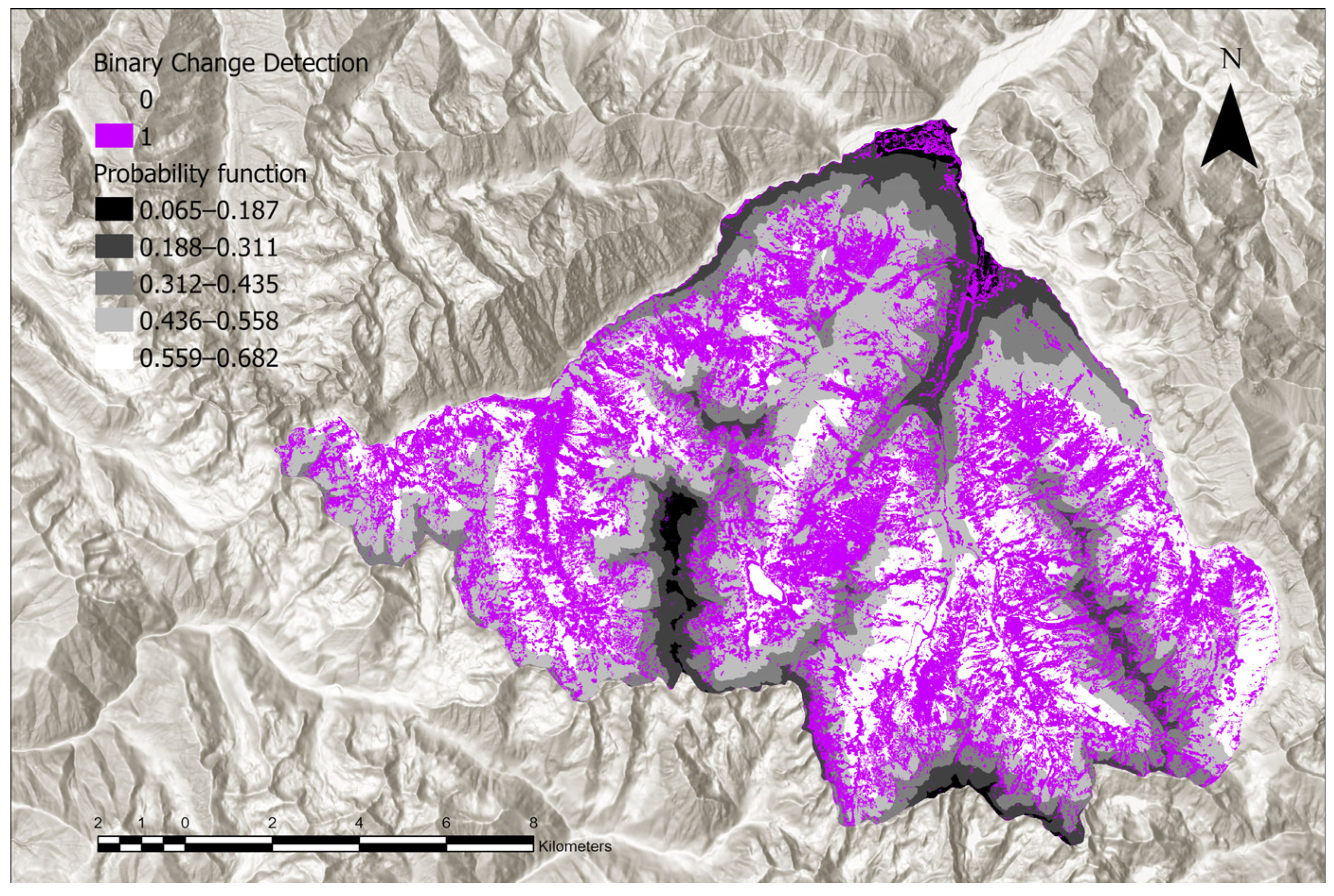
The fitted logistic model was then used to derive a spatial probability map of land cover change, reported in Appendix A. This result confirms what could be interpreted by previous results.
We tested the same model for single transitions; in particular we considered the following changes:
- Permanent herbaceous → Broad-leaved trees;
- Permanent herbaceous → Needle-leaved trees;
- Permanent herbaceous → Low-growing plants;
- Needle-leaved trees → Broad-leaved trees;
- Non- and sparsely- vegetated → Permanent herbaceous;
- Low-growing plants → Needle-leaved trees.
Also in this case, the best model results in the full model with interaction (full+Int) between temperature and elevation (Table 2). The inclusion of interaction terms consistently improved model fit, as indicated by lower AIC values and higher AUC scores.
Table 2.
AIC and AUC parameters for each model and every single transition.
In contrast to the aggregated binary change model, transition-specific models showed substantially higher performance, highlighting that different land-use transitions respond differently to environmental drivers. This indicates that aggregating all changes into a single binary response obscures key ecological processes.
Regarding the influence of the explanatory variables, the results (Table 3) show that temperature anomaly generally increases the probability of land cover transitions, while precipitation anomaly tends to reduce it, except for specific transitions such as low-growing plants (shrubs) to needle-leaved forest. Elevation generally has a negative effect, indicating that most changes occur at lower altitudes, except for the transition involving permanent herbaceous and rock surfaces.
Table 3.
Influence of explanatory variables on single land cover transitions.
The strongest effects were observed for the transition from needle-leaved to broad-leaved forest (OR = 4.40) and from permanent herbaceous to shrub vegetation (OR = 4.69), highlighting a clear shift towards vegetation types adapted to warmer conditions.
Conversely, transitions associated with vegetation recovery, such as shrub to needle-leaved forest, were positively influenced by precipitation (OR = 2.16), suggesting a key role of water availability.
For all transitions, the p-value is lower than 0.001.
Mapping the probability function (Figure 11) for each transition, elevation emerges as the most consistent and influential predictor across transitions, confirming its role as a primary driver structuring land-use dynamics in mountainous environments. In fact, probability maps follow the profile of the DTM raster.
Figure 11.
Probability map for each transition considered for the analysis, where white represents a probability equal to 1, black stands for 0; land cover changes are marked in red: rock to herbaceous (a); needle-leaved trees to broad-leaved trees (b); herbaceous to low-growing plants (c); low-growing plants to needle-leaved trees (d); herbaceous to needle-leaved trees (e); herbaceous to broad-leaved trees (f).
The probability maps highlight spatially structured patterns of land cover change, with higher probabilities concentrated in specific areas of the study region, especially at higher altitudes. These patterns differ among transitions: in particular, the probability maps show more clearly defined spatial patterns for forest-related transitions, particularly from needle-leaved to broad-leaved trees and from shrub or herbaceous vegetation to needle-leaved forest; these transitions appear to be better explained by the combined effect of climate and elevation.
In contrast, transitions involving sparsely vegetated or rocky areas appear more scattered and less spatially structured. This suggests a lower discriminative power of the models for these transitions and indicates that they occur under a wider range of environmental conditions and are likely influenced by additional local factors.
4. Discussions
4.1. Deep Learning Approach for the Classification of High-Resolution Imagery in Alpine Environments
The results addressing RQ1 demonstrate that deep learning-based classification can effectively support land cover mapping from orthoimages in complex alpine environments, although model performance strongly depended on the quality, consistency, and temporal homogeneity of the available datasets. The best-performing configuration, based on the U-Net architecture trained on the CLC + Backbone 2018 dataset [37], achieved substantially higher accuracy than models trained using the standard CLC 2012 inventory, confirming the importance of high-resolution and thematically consistent reference data for semantic segmentation tasks in heterogeneous mountain landscapes. More specifically, the overall accuracy values obtained (82% for AGEA 2018 and 87.76% for ICE 2010 after fine-tuning) are broadly competitive with those reported in the literature for U-Net applied to high-resolution aerial imagery in topographically complex environments, which typically range between 75% and 90% depending on class complexity and training data quality [27]. These results support the conclusion that GIS-integrated deep learning workflows can produce scientifically reliable land cover maps even under operational constraints, provided that the sources of uncertainty are transparently documented and carried through the interpretation of derived products.
However, addressing RQ2, the study highlighted several operational and methodological challenges that are often underestimated in experimental workflows.
One of the main limitations concerned the heterogeneity of the imagery datasets [38]. 2010 and 2018 orthophotos were acquired during summer conditions, whereas the 2021 image was acquired during autumn, in October and November, depending on the frame. These differences likely affected vegetation phenology, illumination conditions, and spectral response, reducing temporal consistency among datasets and limiting model transferability.
Topographic effects represented another major source of uncertainty. Strong shadows, especially in the 2021 orthophoto, frequently caused misclassification between water bodies, rocky surfaces, and vegetation classes. Similar issues were also observed in the 2010 imagery, particularly in the NIR band, which produced unreliable NDVI values. These results confirm that illumination variability and topographic shadowing remain critical limitations for deep learning applications in alpine environments, especially when radiometric normalization and topographic corrections are not applied.
The study also revealed the practical difficulties associated with building multi-temporal datasets for long-term environmental analyses. Several potentially useful datasets could not be included because of corrupted imagery, missing orientation parameters, or incomplete spectral information. Moreover, the available historical series remained relatively short and highly heterogeneous in terms of acquisition conditions and spatial quality. These aspects significantly constrained the temporal robustness of the analysis. However, the proposed methodology could be suitable as a starting point and t0 for future analyses.
From a methodological perspective, since the data used reflect the real conditions frequently encountered by public administrations and protected-area authorities when working with heterogeneous archival datasets and limited computational resources, the workflow intentionally prioritized operational applicability over methodological complexity. No radiometric normalization or advanced preprocessing was applied, and the training samples were manually delineated rather than generated through a statistically rigorous sampling strategy. In addition, a fully independent train–validation–test split was not implemented. While these choices may have affected classification robustness, they also reflect the real conditions frequently encountered by public administrations and protected-area authorities when working with heterogeneous archival datasets and limited computational resources.
Another important aspect concerns the computational demands of the workflow. Although ArcGIS Pro allows non-expert users to implement deep learning procedures within a standard GIS environment, training and inference times remain considerable, especially when processing large, high-resolution orthophotos. Furthermore, the large thematic variability and the relatively high number of classes considered likely reduced class separability, particularly for transitional and heterogeneous land cover categories.
4.2. Land Cover Changes and Climatic Interpretation
Regarding RQ3, the detected land cover transitions reveal a consistent shift towards increased and more structured vegetation cover across the 2010–2021 period. The dominant trajectories include the expansion of broad-leaved deciduous forest, primarily beech, at the expense of needle-leaved forest and low-growing vegetation, as well as the progressive transition from permanent herbaceous to shrub and forest formations. These patterns, observed at both the pixel and class level, are consistent with a process of vegetation densification and upslope biome migration widely documented in alpine ecosystems under warming conditions.
These dynamics align with the thermophilisation process documented across European mountain ranges, whereby warming temperatures favour the competitive advantage of broad-leaved deciduous species such as beech over cold-adapted conifers, and promote shrub encroachment into alpine grasslands as growing season length increases. The warming trend observed in the study area (+0.4 °C/decade) is higher than the current global mean warming rate (+0.17 °C/decade) and closely matches the Italian average (+0.39 °C/decade). This pattern is consistent with the elevation-dependent warming (EDW) theory, according to which high-altitude environments experience amplified warming compared to lower elevations due to snow-albedo feedbacks, atmospheric changes, and topographic effects [39]. Similar vegetation shifts driven by climate warming have been documented not only across the European Alps [40], but also in other different mountainous contexts [41,42].
Addressing RQ4, the logistic regression analysis identified a statistically significant positive association between temperature anomaly and the probability of land cover change (OR = 1.40, 95% CI: 1.23–1.60, p < 0.001), while precipitation anomaly and elevation exerted negative effects (OR ≈ 0.5–0.7). The full model, including the interaction between temperature and elevation, achieved an AUC of 0.63, compared to ≈0.5 for null and topographic-only models. This modest but consistent improvement in discriminatory power suggests that temperature anomalies carry a genuine, if limited, predictive signal for land cover transitions, and that this signal is spatially modulated by elevation. The interaction term was significant and negative (OR = 0.67, p < 0.001), indicating that the effect of temperature on change probability attenuates with increasing altitude. It should be noted, however, that the AUC of 0.63 indicates modest overall discriminatory ability. This result is more appropriately interpreted as evidence of a weak but statistically detectable climatic signal rather than a strong predictive model, particularly given that the change detection raster accumulates classification errors from two independent time points, which may inflate or suppress apparent ecological transitions. This highlights the role of topography in modulating climatic effects and in shaping ecological responses to climate variability, as also reported in mountain ecosystem studies [43,44].
However, these changes should not be interpreted as the direct consequence of temperature increase alone. In mountain environments, land cover dynamics are governed by the interaction of multiple drivers, including climatic conditions, topography, ecological succession, land abandonment, grazing pressure and disturbance regimes [45]. Therefore, the observed transitions reflect a combination of processes rather than a single climatic forcing. Disentangling the relative contribution of each driver lies beyond the scope of the present study, but remains a critical direction for future research. In particular, the availability of land-use management records, grazing cadastres, or forest inventory data for the Valle Gesso area would allow partial attribution of observed transitions to non-climatic drivers and would strengthen the causal interpretation of the detected patterns.
4.3. Operational Implications and Future Perspectives
A distinctive contribution of this study is the development of an end-to-end workflow that integrates deep learning-based land cover classification, multi-temporal change detection, and statistical climate analysis within the ArcGIS Pro environment, without requiring custom coding or specialized deep learning infrastructure. The total processing time of approximately three days on a mid-range workstation (NVIDIA Quadro M2000, 4 GB VRAM) provides a concrete reproducibility benchmark for practitioners considering similar applications. This operational dimension is particularly relevant for protected-area authorities and environmental agencies, which are increasingly mandated to conduct climate impact assessments but operate under constraints of limited computational resources and technical expertise.
The results suggest that even simplified and operationally oriented approaches can provide useful information for environmental monitoring when supported by careful interpretation and awareness of methodological limitations. In this perspective, the study should be interpreted not as a fully optimized deep learning benchmark, but rather as an experimental operational framework developed under real-world data constraints. Transparency regarding uncertainty sources, including seasonal inconsistency between acquisitions, absence of radiometric normalization, and non-independent validation, is a prerequisite for the responsible use of such workflows in decision support contexts.
Future developments should focus on three prioritized directions. First, and most impactful, is the application of topographic shadow correction and radiometric normalization to the AGEA 2021 orthophoto. Given that autumn acquisition conditions introduced pervasive shadow effects that propagated through both the pixel classification and the change detection layers, correcting this single dataset is expected to yield the largest improvement in overall accuracy and temporal consistency. Ongoing work is addressing this through C-correction and shadow masking techniques [46,47].
Second, methodological robustness should be strengthened through a fully independent train–validation–test split and a stratified random sampling strategy for validation points, replacing the current expert-driven delineation. Third, the statistical modelling of land cover change should be extended to include non-climatic explanatory variables such as slope, aspect, distance to forest edge, and, where available, land management indicators, so as to reduce the residual unexplained variance and to isolate the specific contribution of climate anomalies from confounding ecological and anthropogenic drivers. Transferability testing across comparable alpine areas, such as the adjacent French Mercantour National Park, would allow evaluation of how well the trained models generalize to different sensor configurations, acquisition dates, and ecological gradients. Such cross-border validation would be particularly relevant within the ALCOTRA cooperation framework, and would provide a more robust basis for scaling the workflow to regional monitoring programmes. Public release of the workflow documentation and training data, for example via Zenodo, would further support reproducibility and facilitate independent evaluation by other research groups. Finally, recent advances in geospatial foundation models and transformer-based architectures offer new opportunities for improving classification performance and reducing dependence on labelled data. The integration of these approaches represents a promising direction for future developments.
5. Conclusions
This study investigated the application of deep learning algorithms for the pixel-based classification of high-resolution aerial imagery in a selected mountainous sector of Gesso Valley. The workflow, implemented within ArcGIS Pro without custom programming, integrates U-Net-based pixel classification of multi-temporal RGB–NIR orthophotos (2010, 2018, 2021), categorical change detection, climate anomaly analysis based on 28 weather stations over 1990–2021, and logistic regression modelling of land cover transitions as a function of temperature and precipitation anomalies and elevation. The results showed that satisfactory classification performances can be achieved even under heterogeneous and non-ideal data conditions, particularly when using higher-resolution and thematically consistent training datasets. The detected land cover transitions revealed a general increase in vegetation cover and highlighted statistically significant relationships between climate anomalies and land cover dynamics, although these processes are influenced by multiple interacting environmental and anthropogenic drivers.
Beyond the specific results obtained for Gesso Valley, the study highlights the importance of addressing the practical challenges associated with multi-temporal environmental monitoring in mountain regions, including data heterogeneity, spectral inconsistencies, shadow effects, and limited temporal availability of historical datasets. In this perspective, the proposed workflow should be interpreted as an operational and transferable framework developed under real-world conditions rather than as a fully optimized deep learning benchmark.
Despite the identified limitations, the obtained results are broadly coherent with the current literature on alpine vegetation dynamics and demonstrate that GIS-integrated deep learning approaches can support environmental monitoring activities also in contexts where advanced artificial intelligence expertise and highly standardized datasets are not available.
Future developments will focus on improving radiometric and topographic consistency among datasets, extending the temporal depth of the analysis, integrating additional environmental variables, and testing the transferability of the workflow to other alpine regions. In parallel, the integration of geospatial foundation models and transformer-based architectures into the GIS-embedded workflow represents a promising avenue to reduce dependence on labelled training data and to improve generalization across heterogeneous acquisition conditions.
Author Contributions
Conceptualization, C.G. and F.M.; methodology, C.G., F.M. and A.M.L.; software, C.G.; validation, C.G., F.M. and A.M.L.; formal analysis, C.G.; investigation, C.G., and F.M.; resources, F.M.; data curation, C.G. and F.M.; writing—original draft preparation, C.G.; writing—review and editing, C.G., F.M. and A.M.L.; visualization, C.G. and F.M.; supervision, F.M. and A.M.L.; project administration, F.M.; funding acquisition, F.M. and A.M.L. All authors have read and agreed to the published version of the manuscript.
Funding
The project was part of a collaboration with the Alpi Marittime Protected Areas (APAM) and was funded by the Interreg VI-A France–Italy ALCOTRA 2021–2027 Programme, project no. 20138 “ACLIMO”.
Data Availability Statement
The datasets used in this study are partly publicly available and partly provided by institutional sources. High-resolution orthophotos and Digital Terrain Models (DTMs) were provided by the Geoportale Piemonte. Meteorological data used in this study were obtained from ARPA Piemonte (Regional Environmental Protection Agency), which provides open-access environmental monitoring data. Additional data generated or analyzed during this study are available from the authors upon reasonable request.
Acknowledgments
The authors would like to thank Stefano Campus of the Piedmont Region, SITA sector, for his valuable support and collaboration, particularly in facilitating data access and contributing to the development of the study. We also acknowledge Luca Gautero, Costanza Luconi, Daniela Quaranta, Laura Martinelli and other staff and operators of Aree Protette Alpi Marittime (APAM) for their essential contribution and for their support in the interpretation and validation of the results within the ACLIMO project framework. Finally, the authors would like to thank Bartolomeo Vigna and Adriano Fiorucci from Politecnico di Torino for their collaboration on the climate analysis, in particular for the elaboration and the interpretation of weather data.
Conflicts of Interest
The authors declare no conflicts of interest.
Abbreviations
The following abbreviations are used in this manuscript:
| GIS | Geographic Information System |
| RS | Remote Sensing |
| DL | Deep Learning |
| CNN | Convolutional Neural Network |
| LULC | Land Use and Land Cover |
| ALCOTRA | Alpi Latine COoperazione TRAnsfrontaliera |
| APAM | Aree Protette Alpi Marittime |
| DEM | Digital Elevation Model |
| RGB | Red, Green, Blue |
| NIR | Near-Infrared |
| DTM | Digital Terrain Model |
| DSM | Digital Surface Model |
| AGEA | Agenzia per le Erogazioni in Agricoltura |
| NDVI | Normalized Difference Vegetation Index |
| ExG | Excess Green Index |
| CLC | CORINE Land Cover |
| MMU | Minimum Mapping Unit |
| MMW | Minimum Mapping Width |
| ARPA | Agenzia Regionale per la Protezione Ambientale |
| ROI | Region Of Interest |
| OA | Overall Accuracy |
| GAM | Generalized Additive Model |
| EBK | Empirical Bayesian Kriging |
| AIC | Akaike Information Criterion |
| AUC | Area Under the Curve |
| OR | Odds Ratio |
| CI | Confidence Interval |
| ME | Mean Error |
| RMSE | Root Mean Square Error |
| MAE | Mean Absolute Error |
Appendix A
This appendix provides additional figures supporting the results presented in the main text.
Figure A1.
Digital Terrain Model.
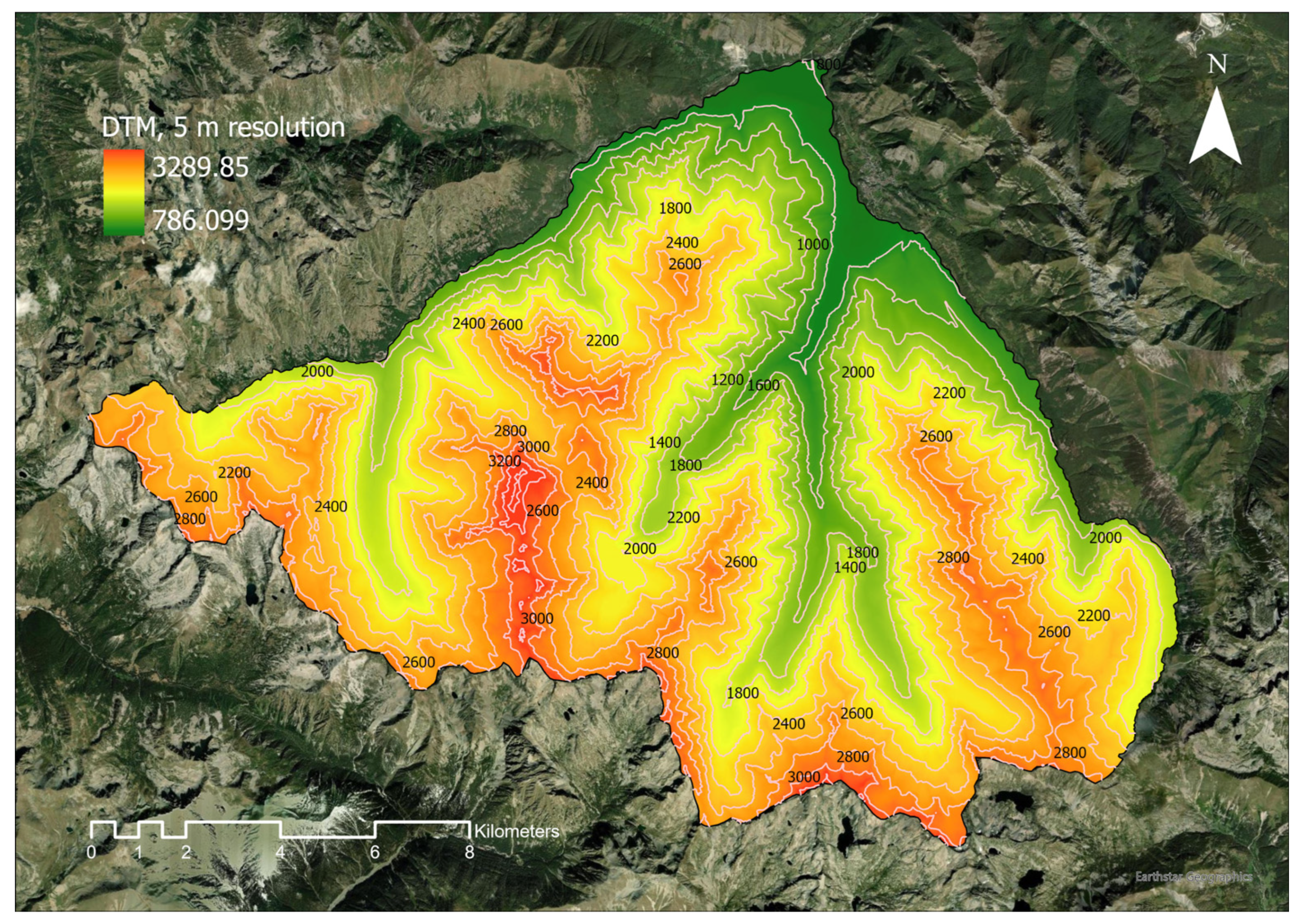
Figure A2.
NDVI calculated from orthophoto ICE 2010.
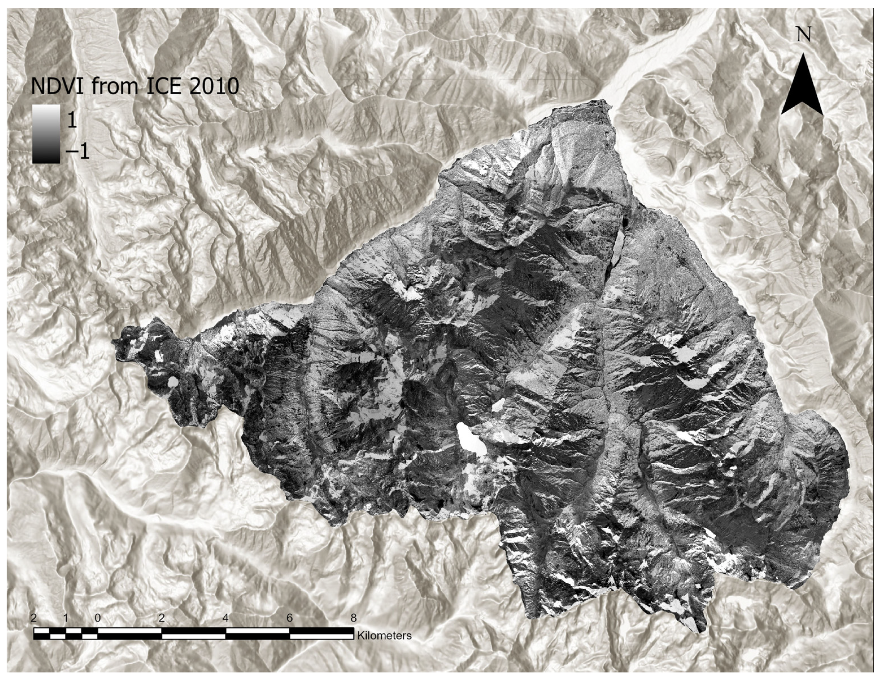
Figure A3.
ExG calculated from orthophoto ICE 2010.
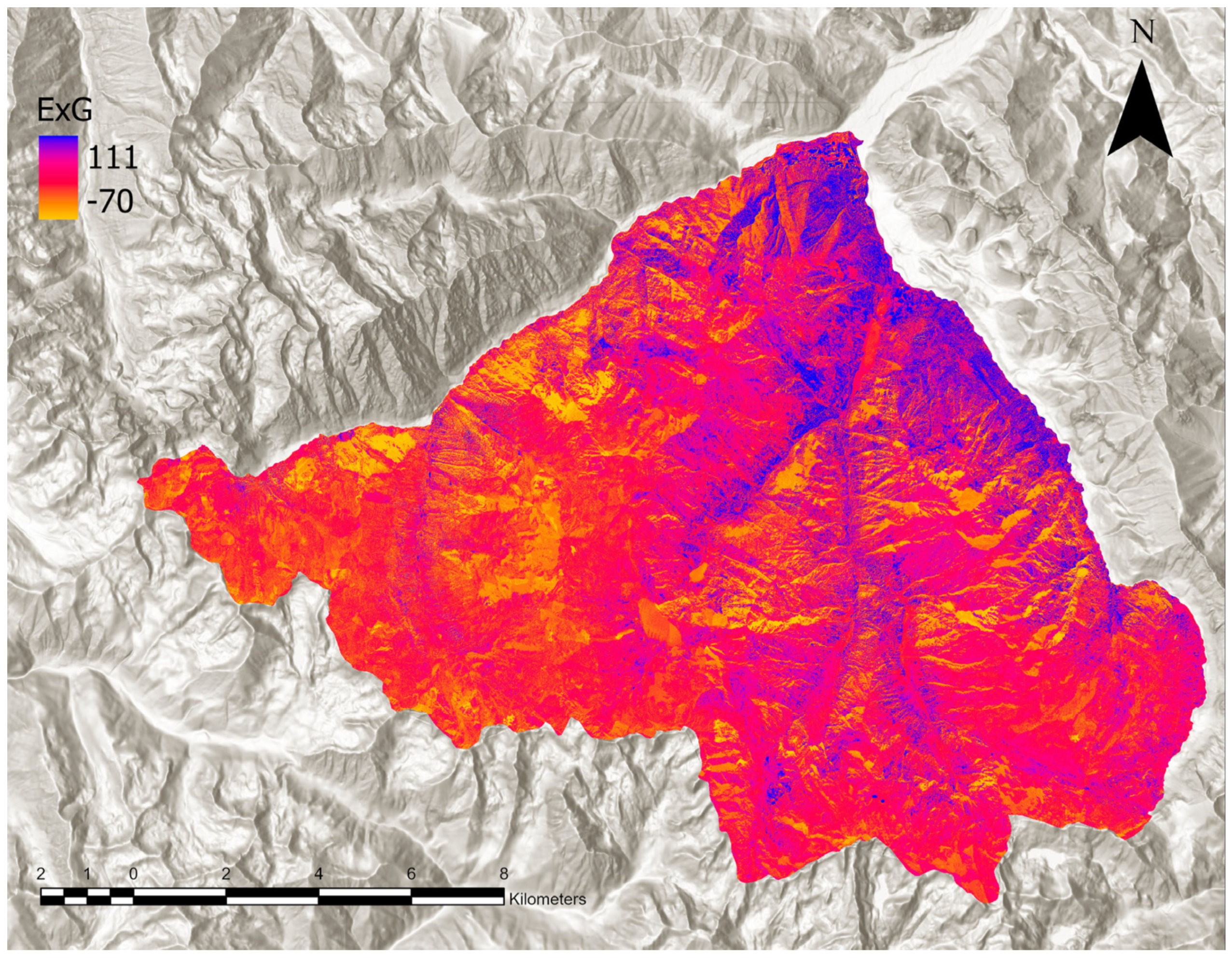
Figure A4.
NDVI calculated from orthophoto AGEA 2018.
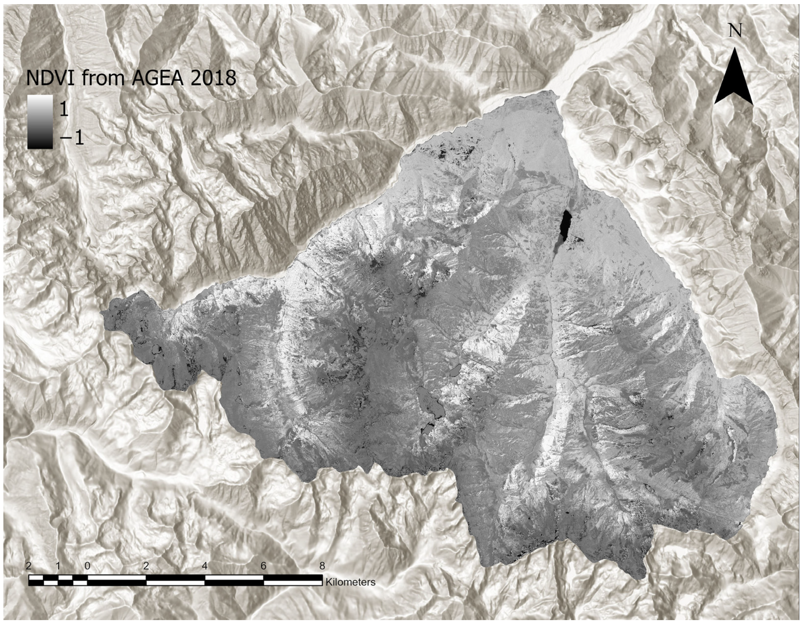
Figure A5.
CORINE Land Cover 2012 classes.
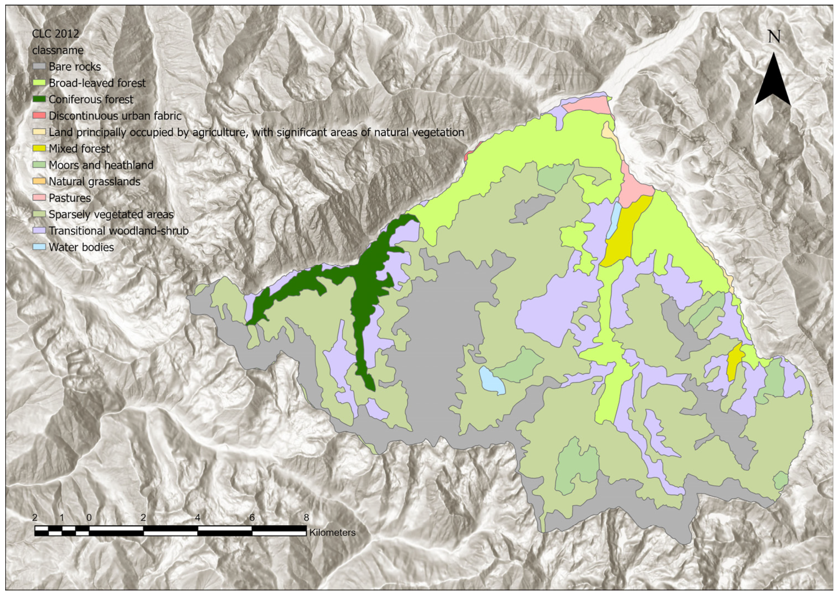
Figure A6.
CORINE Land Cover 2018 + backbone classes.
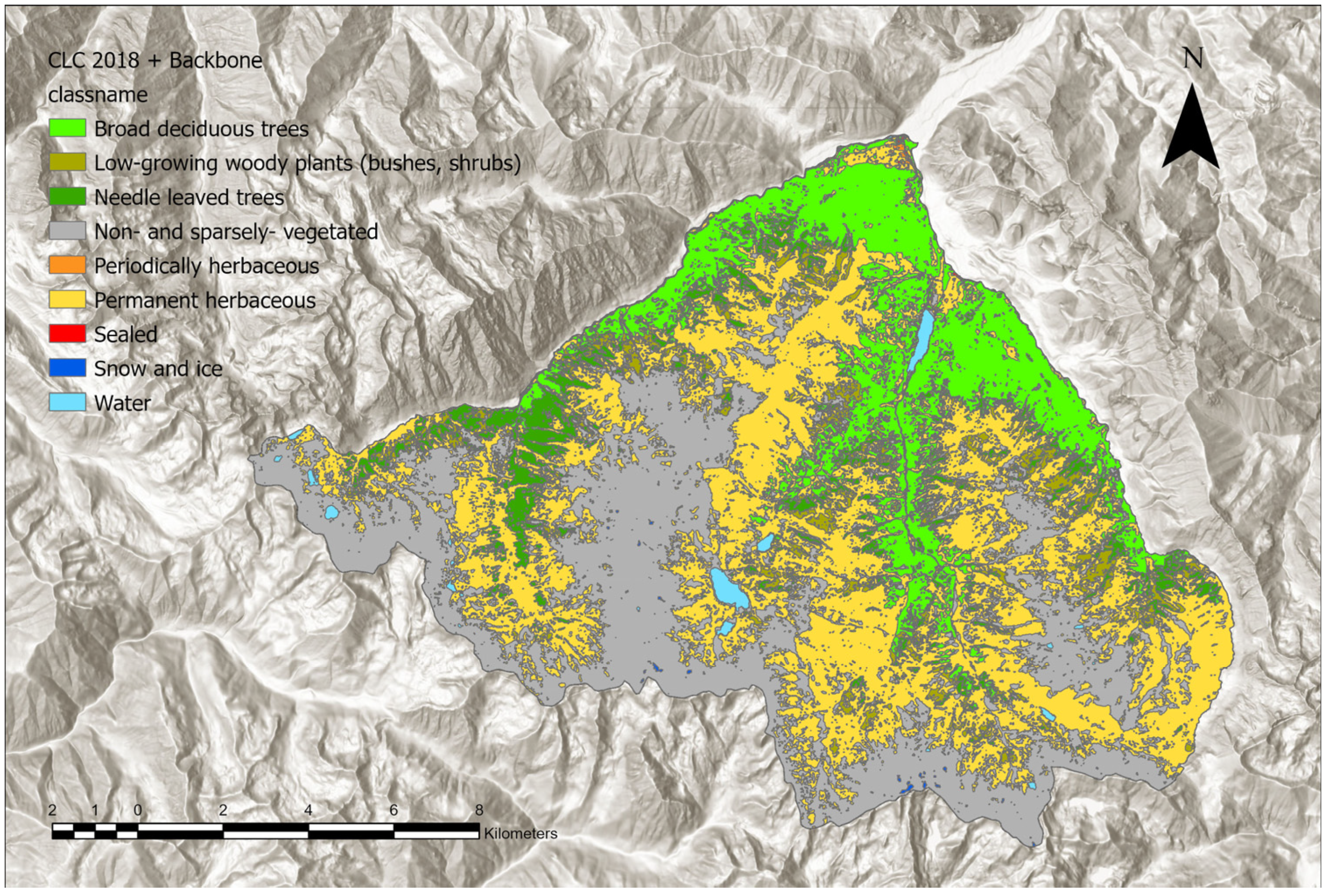
Figure A7.
Seasonal temperature anomalies for 1990–2021 relative to the 2000–2021 baseline.
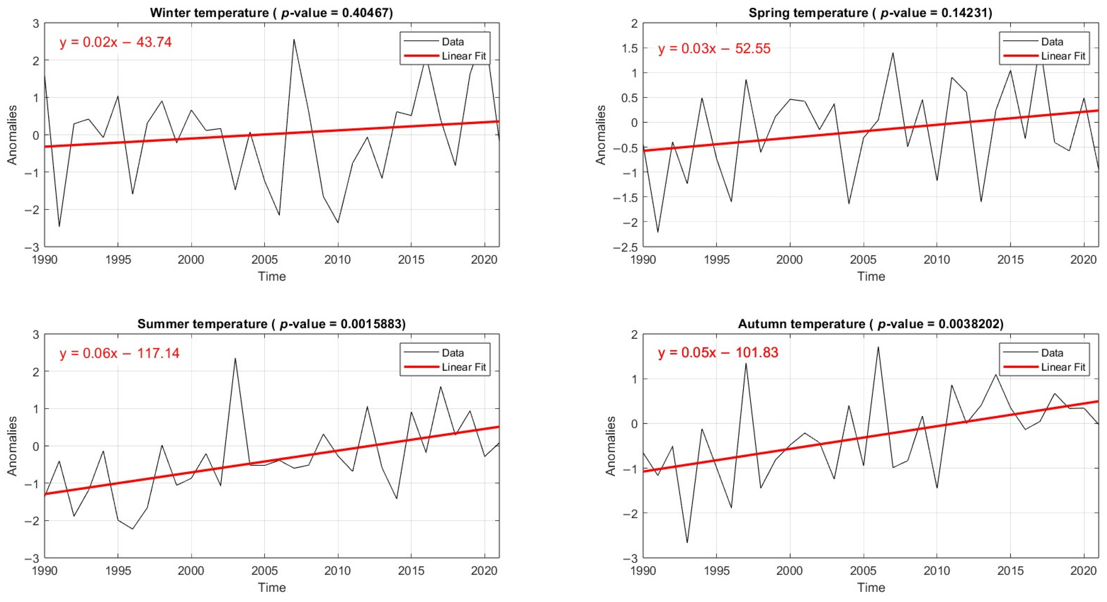
Figure A8.
Seasonal precipitation anomalies for 1990–2021 relative to the 2000–2021 baseline. Positive anomalies (blue bars) indicate wetter-than-average conditions, while negative anomalies (red bars) indicate drier-than-average conditions.
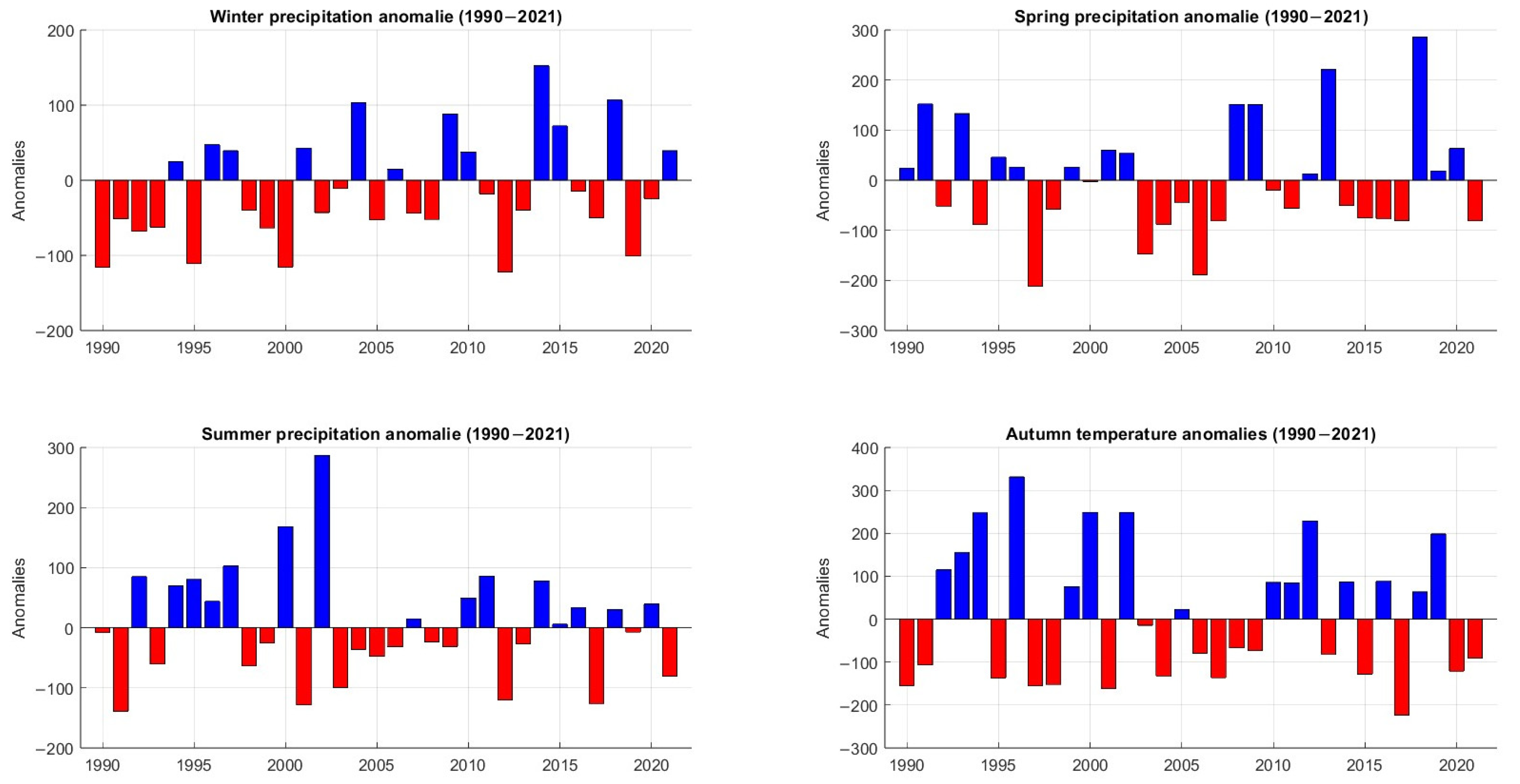
Figure A9.
Probability function map (grey scale) overlapped by the binary change detection raster, where changes are shown in purple. Most of the changes fall under the probability range 0.44–0.68.
Appendix B
This appendix provides additional tables supporting the results presented in the main text.
Table A1.
Original dataset employed for the analysis.
Table A2.
CLC 2012 classes at three levels of hierarchy.
Table A3.
ARPA Piemonte weather stations information about the altitude where the station is located, the time period of data acquisition and which parameters were registered (daily temperature, maximum and minimum temperature, daily precipitation).
Table A4.
CNN’s parameters.
Table A5.
Confusion matrix parameters for the best classifier. C_number represents the code of the land cover class: 1 for sealed; 2 for needle-leaved trees; 3 for broad-leaved deciduous trees; 4 for low-growing woody plants; 5 for permanent herbaceous; 6 for periodically herbaceous; 7 for non- and sparsely-vegetated areas; 8 for water; and 9 for snow and ice. Colors are meant to highlight the diagonal of the matrix (green), especially the overall accuracy (yellow) and the Kappa coefficient (cyan).
Table A6.
EBK and GAM metrics for temperature anomaly.
Table A7.
EBK and GAM metrics for precipitation anomaly.
Table A8.
AIC and AUC parameters for the evaluation of logistic regression models.
Table A9.
Parameters of the coefficients.
References
- Beaumet, J.; Ménégoz, M.; Morin, S.; Gallée, H.; Fettweis, X.; Six, D.; Vincent, C.; Wilhelm, B.; Anquetin, S. Twentieth century temperature and snow cover changes in the French Alps. Reg. Environ. Change 2021, 21, 114. [Google Scholar] [CrossRef] [Scilit]
- Scherrer, S.C.; Hirschi, M.; Spirig, C.; Maurer, F.; Kotlarski, S. Trends and drivers of recent summer drying in Switzerland. Environ. Res. Commun. 2022, 4, 02500. [Google Scholar] [CrossRef] [Scilit]
- Kotlarski, S.; Gobiet, A.; Morin, S.; Olefs, M.; Rajczak, J.; Samacoïts, R. 21st Century alpine climate change. Clim. Dyn. 2021, 60, 65–86. [Google Scholar] [CrossRef] [Scilit]
- European Environment Agency (EEA). Regional Climate Change and Adaptation: The Alps Facing the Challenge of Changing Water Resources. In EEA Reports; European Environment Agency (EEA): Copenhagen, Denmark, 2009. [Google Scholar]
- Majeed, M.; Tariq, A.; Anwar, M.M.; Khan, A.M.; Arshad, F.; Mumtaz, F.; Farhan, M.; Zhang, L.; Zafar, A.; Aziz, M.; et al. Monitoring of Land Use–Land Cover Change and Potential Causal Factors of Climate Change in Jhelum District, Punjab, Pakistan, through GIS and Multi-Temporal Satellite Data. Land 2021, 10, 1026. [Google Scholar] [CrossRef] [Scilit]
- Dedieu, J.P.; Lessard-Fontaine, A.; Ravazzani, G.; Cremonese, E.; Shalpykova, G.; Beniston, M. Shifting mountain snow patterns in a changing climate from remote sensing retrieval. Sci. Total Environ. 2014, 493, 1267–1279. [Google Scholar] [CrossRef] [Scilit] [PubMed]
- Yuan, Q.-Q.; Shen, H.; Li, T.; Li, Z.; Li, S.; Jiang, Y.; Xu, H.; Tan, W.; Yang, Q.; Wang, J.; et al. Deep learning in environmental remote sensing: Achievements and challenges. Remote Sens. Environ. 2020, 241, 111716. [Google Scholar] [CrossRef] [Scilit]
- Deressu, T.F.; Bojer, A.K.; Debelee, T.G.; Negera, W.G.; Nadarajah, S.; Gebissa, K.W. Enhancing land use and land cover classification with deep learning-based satellite imagery segmentation. Int. J. Appl. Earth Obs. Geoinf. 2025, 144, 104839. [Google Scholar] [CrossRef] [Scilit]
- Dozier, J.; Bair, E.H.; Baskaran, L.; Brodrick, P.G.; Carmon, N.; Kokaly, R.F.; Miller, C.E.; Miner, K.R.; Painter, T.H.; Thompson, D.R. Error and Uncertainty Degrade Topographic Corrections of Remotely Sensed Data. J. Geophys. Res. Biogeosciences 2022, 127, e2022JG007147. [Google Scholar] [CrossRef] [Scilit]
- Tuia, D.; Persello, C.; Bruzzone, L. Domain adaptation for the classification of remote sensing data: An overview of recent advances. IEEE Geosci. Remote Sens. Mag. 2016, 4, 41–57. [Google Scholar] [CrossRef] [Scilit]
- Geneviève, D. Artificial Intelligence: Opportunities and Challenges for Public Administration. Can. Public Adm. 2024, 67, 388–406. [Google Scholar] [CrossRef] [Scilit]
- Ma, L.; Liu, Y.; Zhang, X.; Ye, Y.; Yin, G.; Johnson, B.A. Deep learning in remote sensing applications: A meta-analysis and review. ISPRS J. Photogramm. Remote Sens. 2019, 152, 166–177. [Google Scholar] [CrossRef] [Scilit]
- Biagi, S.; Fortunato, T.; Porcari, S.; Priore, A. Integrated Workflow for Public Administration: From Data Collection to the Management Platform for Built Heritage. Emerg. Perspect. Built Environ. 2026, 125–143. [Google Scholar] [CrossRef] [Scilit]
- Aree Protette Delle Alpi Marittime. Available online: https://www.marittimemercantour.eu/territorio/aree-protette-delle-alpi-marittime (accessed on 24 February 2026).
- Aree Protette Alpi Marittime-Ente di Gestione. Montagne. Available online: https://www.parcoalpimarittime.it/conosci-il-parco/geologia/montagne (accessed on 25 January 2026).
- Regione Piemonte. Elenco Delle Regioni Eco-Geografiche Proposte Per La Regione Piemonte. Available online: https://www.regione.piemonte.it/giscartografia/Parchi/schede_settori_ecogeografici.pdf (accessed on 5 May 2026).
- Aree Protette Alpi Marittime-Ente di Gestione. Ghiacciai. Available online: https://www.parcoalpimarittime.it/conosci-il-parco/geologia/ghiacciai (accessed on 25 January 2026).
- Aree Protette Alpi Marittime-Ente di Gestione. Boschi. Available online: https://www.parcoalpimarittime.it/conosci-il-parco/flora/boschi (accessed on 25 January 2026).
- RIPRESA AEREA ICE 2009-2011-DTM 5. Available online: https://www.geoportale.piemonte.it/geonetwork/srv/ita/catalog.search#/metadata/r_piemon:224de2ac-023e-441c-9ae0-ea493b217a8e (accessed on 12 March 2024).
- Haggag, W.; Ali, R.R.; Al-Ansary, N.A. Geographic information systems and remote sensing: Innovative tools for plant health. Int. J. Agric. Technol. 2023, 19, 2449–2464. [Google Scholar]
- Yang, M.-D.; Tseng, H.-H.; Hsu, Y.-C.; Tsai, H.P. Semantic Segmentation Using Deep Learning with Vegetation Indices for Rice Lodging Identification in Multi-date UAV Visible Images. Remote Sens. 2020, 12, 633. [Google Scholar] [CrossRef] [Scilit]
- Gallardo, M.; Cocero, D. Using the European CORINE Land Cover Database: A 2011–2021 Specific Review. In Sustainable Development Goals in Europe. Key Challenges in Geography; De Lázaro Torres, M.L., De Miguel González, R., Eds.; Springer: Cham, Switzerland, 2023; pp. 303–325. [Google Scholar] [CrossRef] [Scilit]
- CORINE Land Cover. Available online: https://land.copernicus.eu/en/products/corine-land-cover (accessed on 15 March 2024).
- Banca Dati Storica. Available online: https://www.arpa.piemonte.it/rischi_naturali/snippets_arpa_graphs/map_meteoweb/ (accessed on 24 February 2026).
- ESRI. Deep Learning Using the ArcGIS Image Analyst Extension. Available online: https://doc.esri.com/en/arcgis-pro/latest/help/analysis/image-analyst/deep-learning-in-arcgis-pro.html (accessed on 20 May 2026).
- ARPA Piemonte. Zone Umide. Available online: https://www.arpa.piemonte.it/scheda-informativa/zone-umide (accessed on 18 May 2026).
- Clark, A.; Phinn, S.; Scarth, P. Optimised U-Net for Land Use–Land Cover Classification Using Aerial Photography. PFG–J. Photogramm. Remote Sens. Geoinf. Sci. 2023, 91, 125–147. [Google Scholar] [CrossRef] [Scilit]
- ESRI. Compute Confusion Matrix (Spatial Analyst). Available online: https://pro.arcgis.com/en/pro-app/3.4/tool-reference/spatial-analyst/compute-confusion-matrix.htm (accessed on 20 May 2026).
- ESRI. Change Detection Wizard. Available online: https://pro.arcgis.com/en/pro-app/3.6/help/analysis/image-analyst/the-change-detection-wizard.htm (accessed on 20 May 2026).
- Mercalli, L.; Berro, D.C. Ultimi Ghiacci. Clima e Ghiacciai nelle Alpi Marittime; Edizioni Società Meteorologica Subalpina: Moncalieri, Italy, 2019. [Google Scholar]
- Aalto, J.; Pirinen, P.; Heikkinen, J.; Venalainen, A. Spatial interpolation of monthly climate data for Finland: Comparing the performance of kriging and generalized additive models. Theor. Appl. Climatol. 2013, 112, 99–111. [Google Scholar] [CrossRef] [Scilit]
- Nteranya, J.N.; Kiplagat, A.; Ucakuwun, E.K.; Nzabandora, C.K. Land use/land cover (LULC) changes modeling and susceptibility mapping using the binary logistic regression at the territorial level in eastern DR Congo. J. Degrad. Min. Lands Manag. 2024, 11, 6399–6411. [Google Scholar] [CrossRef] [Scilit]
- Yanagihara, H.; Kamo, K.I.; Imori, S.; Satoh, K. Bias-corrected AIC for selecting variables in multinomial logistic regression models. Linear Algebra Its Appl. 2012, 436, 4329–4341. [Google Scholar] [CrossRef] [Scilit]
- Austin, P.C.; Steyerberg, E.W. Interpreting the concordance statistic of a logistic regression model: Relation to the variance and odds ratio of a continuous explanatory variable. BMC Med. Res. Methodol. 2012, 12, 82. [Google Scholar] [CrossRef] [Scilit]
- Li, Q.; Wei, Y.; Zhang, T.; Che, F.; Yao, S.; Wang, C.; Shi, D.D.; Tang, H.H.; Song, B. Predictive models and early postoperative recurrence evaluation for hepatocellular carcinoma based on gadoxetic acid-enhanced MR imaging. Insights Imaging 2023, 14, 4. [Google Scholar] [CrossRef] [Scilit]
- Regione Piemonte. Scenari Climatici. 2022. Available online: https://www.regione.piemonte.it/web/sites/default/files/media/documenti/2022-03/climatt_scenari.pdf (accessed on 8 June 2024).
- Vitasse, Y.; Ursenbacher, S.; Klein, G.; Bohnenstengel, T.; Chittaro, Y.; Delestrade, A.; Monnerat, C.; Rebetez, M.; Rixen, C.; Strebel, N.; et al. Phenological and elevational shifts of plants, animals and fungi under climate change in the European Alps. Biol. Rev. 2021, 96, 1816–1835. [Google Scholar] [CrossRef] [Scilit]
- Ulmas, P.; Liiv, I. Segmentation of satellite imagery using u-net models for land cover classification. arXiv 2020, arXiv:2003.02899. [Google Scholar] [CrossRef] [Scilit]
- Mountain Research Initiative EDW Working Group. Elevation-dependent warming in mountain regions of the world. Nat. Clim. Chang. 2015, 5, 424–430. [Google Scholar] [CrossRef] [Scilit]
- Whang, S.E.; Lee, J.G. Data collection and quality challenges for deep learning. Proc. VLDB Endow. 2020, 13, 3429–3432. [Google Scholar] [CrossRef] [Scilit]
- Luo, Y.; Ma, N.; Zhang, Y.; Zang, C.; Szilagyi, J.; Tian, J.; Wang, L.; Xu, Z.; Tang, Z.; Wei, H. Response of alpine vegetation function to climate change in the Tibetan Plateau: A perspective from solar-induced chlorophyll fluorescence. Sci. Total Environ. 2024, 952, 175845. [Google Scholar] [CrossRef] [Scilit] [PubMed]
- Chen, J.M.; Ju, W.; Ciais, P.; Viovy, N.; Liu, R.; Liu, Y.; Lu, X. Vegetation structural change since 1981 significantly enhanced the terrestrial carbon sink. Nat. Commun. 2019, 10, 4259. [Google Scholar] [CrossRef] [Scilit] [PubMed]
- Macek, M.; Kopecký, M.; Wild, J. Maximum air temperature controlled by landscape topography affects plant species composition in temperate forests. Landsc. Ecol. 2019, 34, 2541–2556. [Google Scholar] [CrossRef] [Scilit]
- Giaccone, E.; Luoto, M.; Vittoz, P.; Guisan, A.; Mariéthoz, G.; Lambiel, C. Influence of microclimate and geomorphological factors on alpine vegetation in the Western Swiss Alps. Earth Surf. Process. Landf. 2019, 44, 3093–3107. [Google Scholar] [CrossRef] [Scilit]
- Filippa, G.; Cremonese, E.; Galvagno, M.; Isabellon, M.; Bayle, A.; Choler, P.; Carlson, B.Z.; Gabellani, S.; Morra di Cella, U.; Migliavacca, M. Climatic Drivers of Greening Trends in the Alps. Remote Sens. 2019, 11, 2527. [Google Scholar] [CrossRef] [Scilit]
- Reese, H.; Olsson, H. C-correction of optical satellite data over alpine vegetation areas: A comparison of sampling strategies for determining the empirical c-parameter. Remote Sens. Environ. 2011, 115, 1387–1400. [Google Scholar] [CrossRef] [Scilit]
- Xu, H.; Zhu, J.; Wang, F.; You, H.; Wang, W. A Shadow Detection Method Combining Topography and Spectra for Remote Sensing Images in Mountainous Environments. Appl. Sci. 2025, 15, 4899. [Google Scholar] [CrossRef] [Scilit]
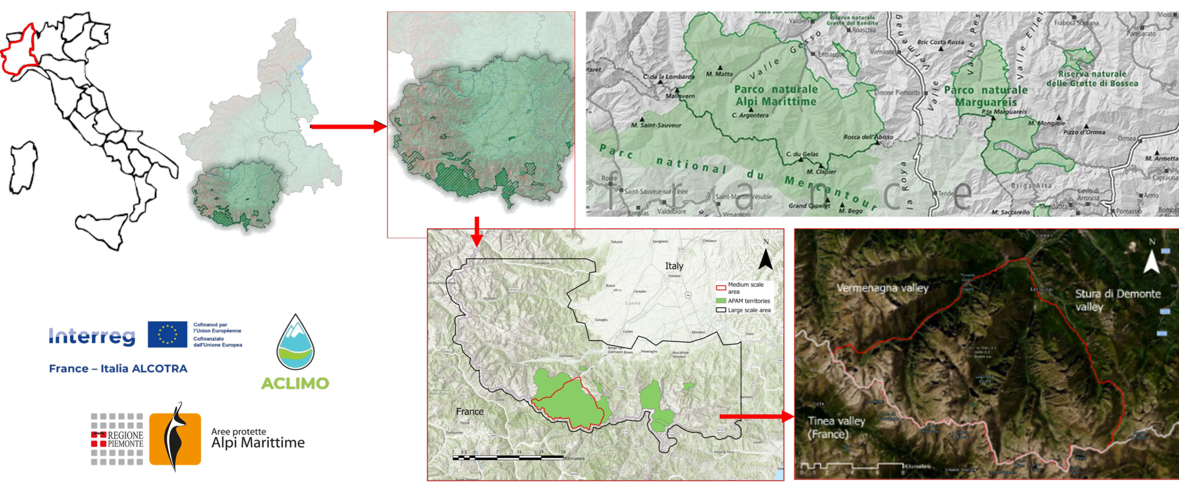
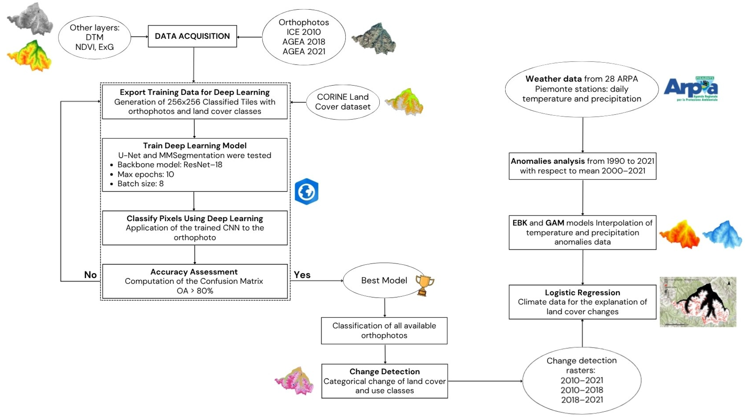
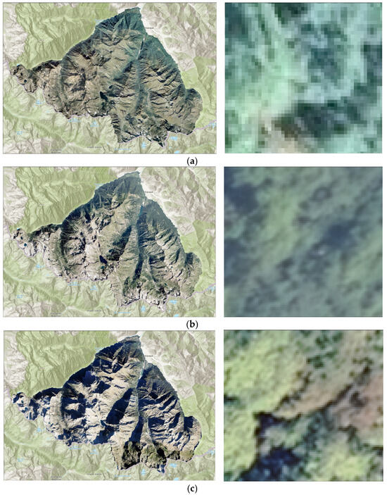
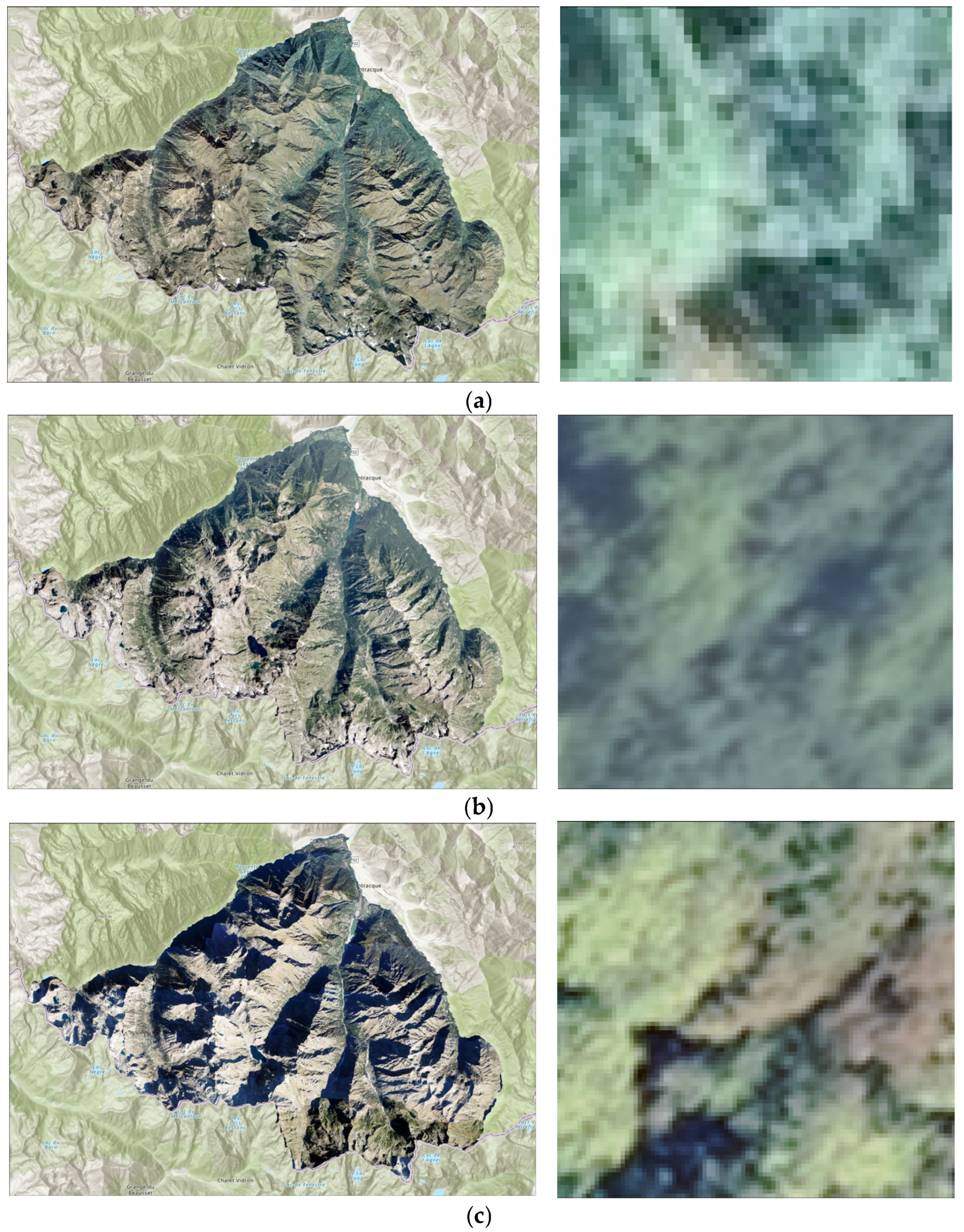
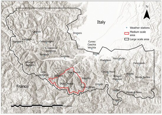
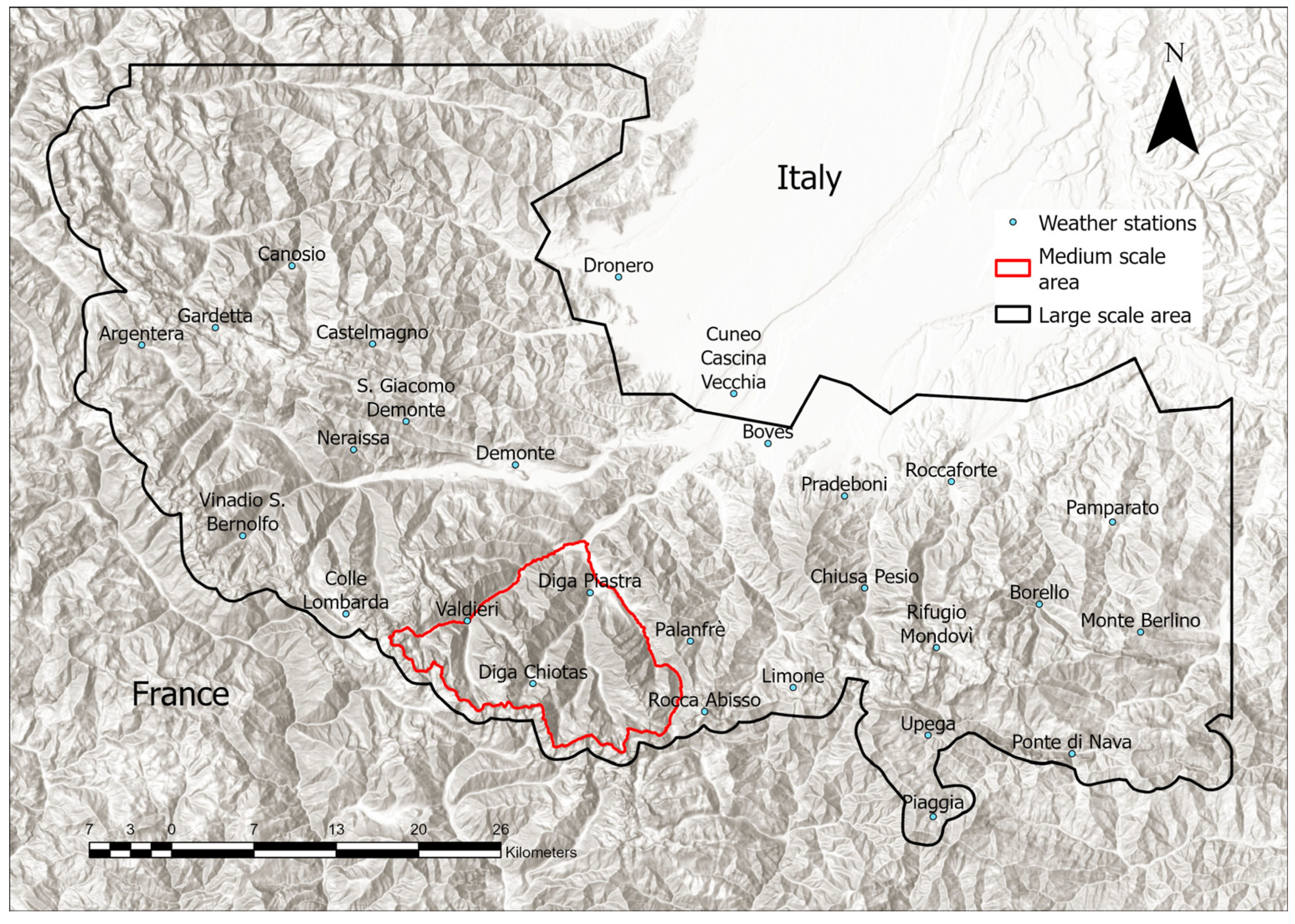
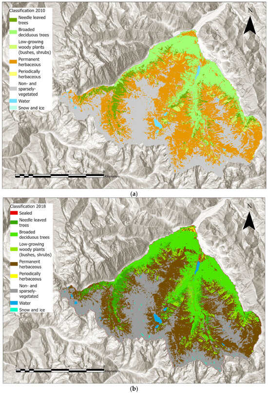
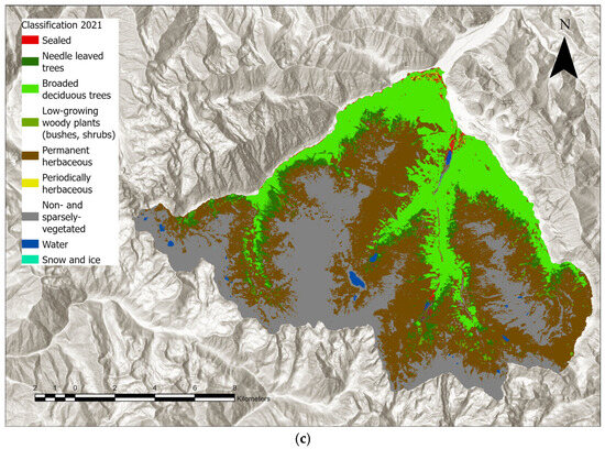
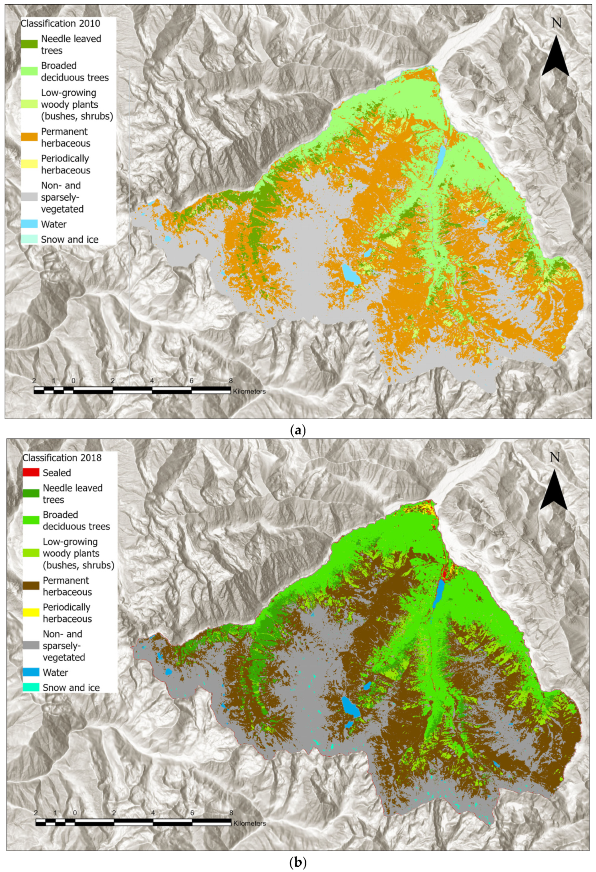
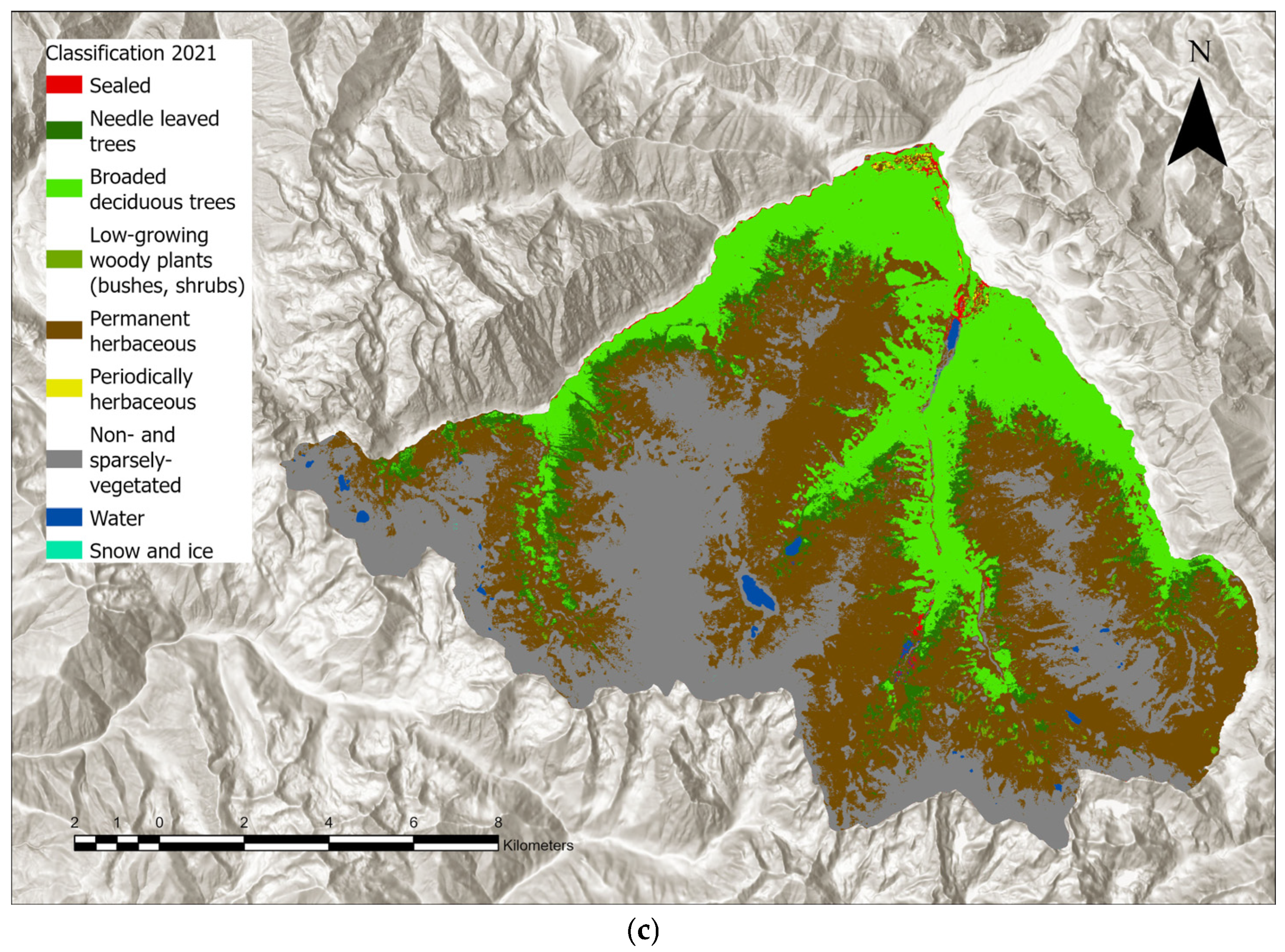
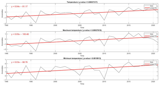
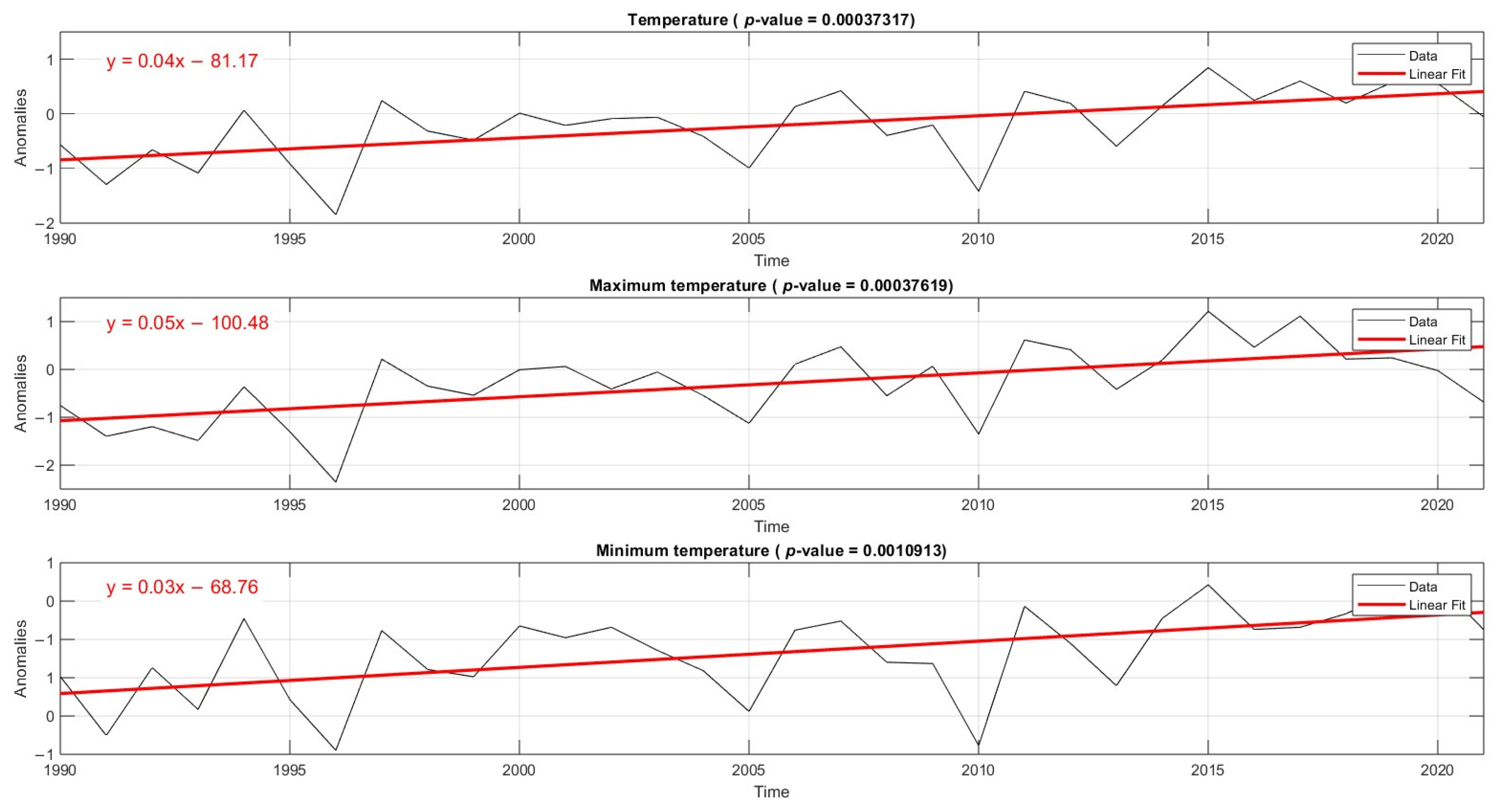
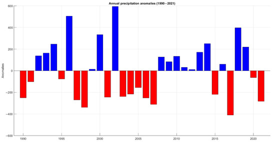
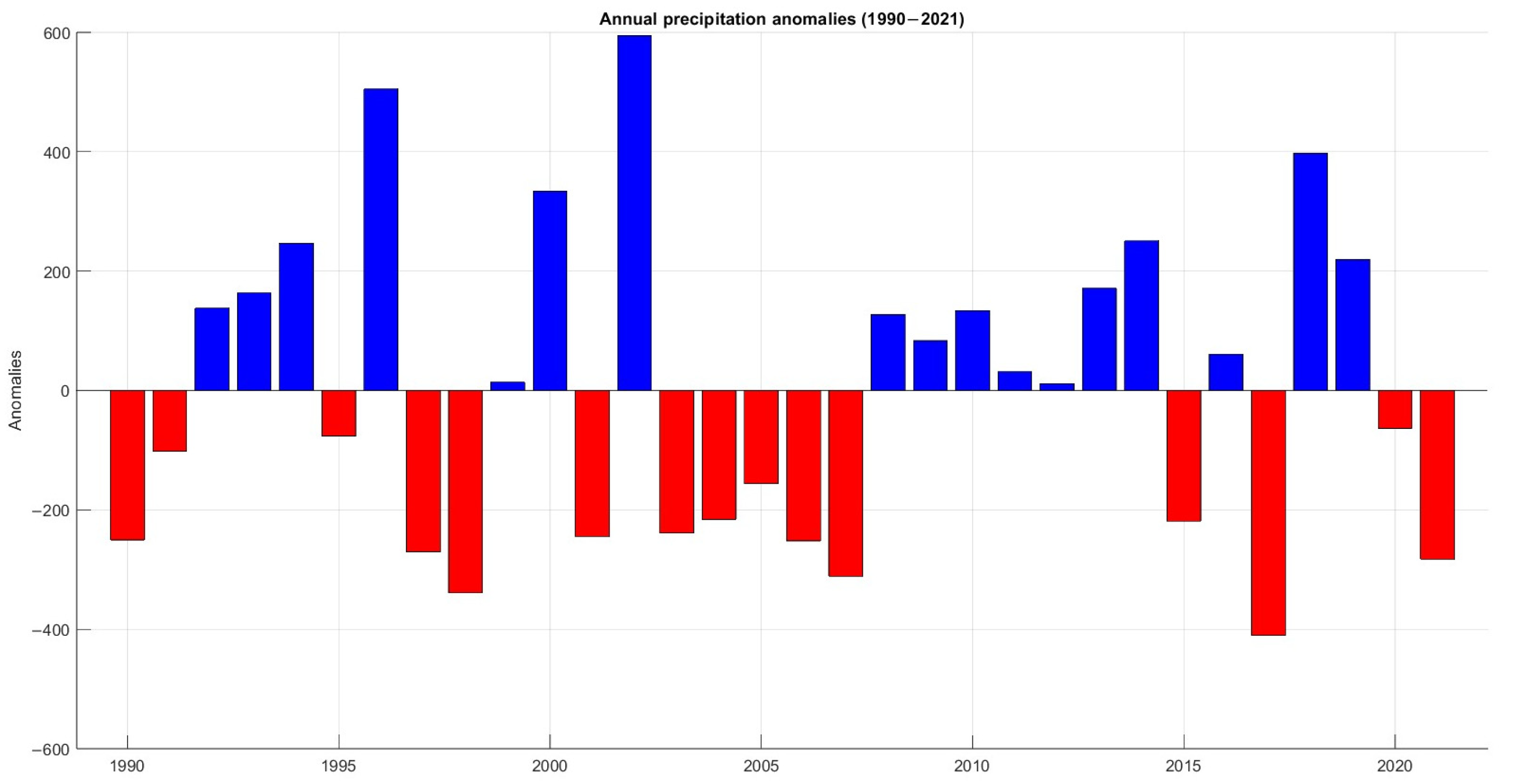
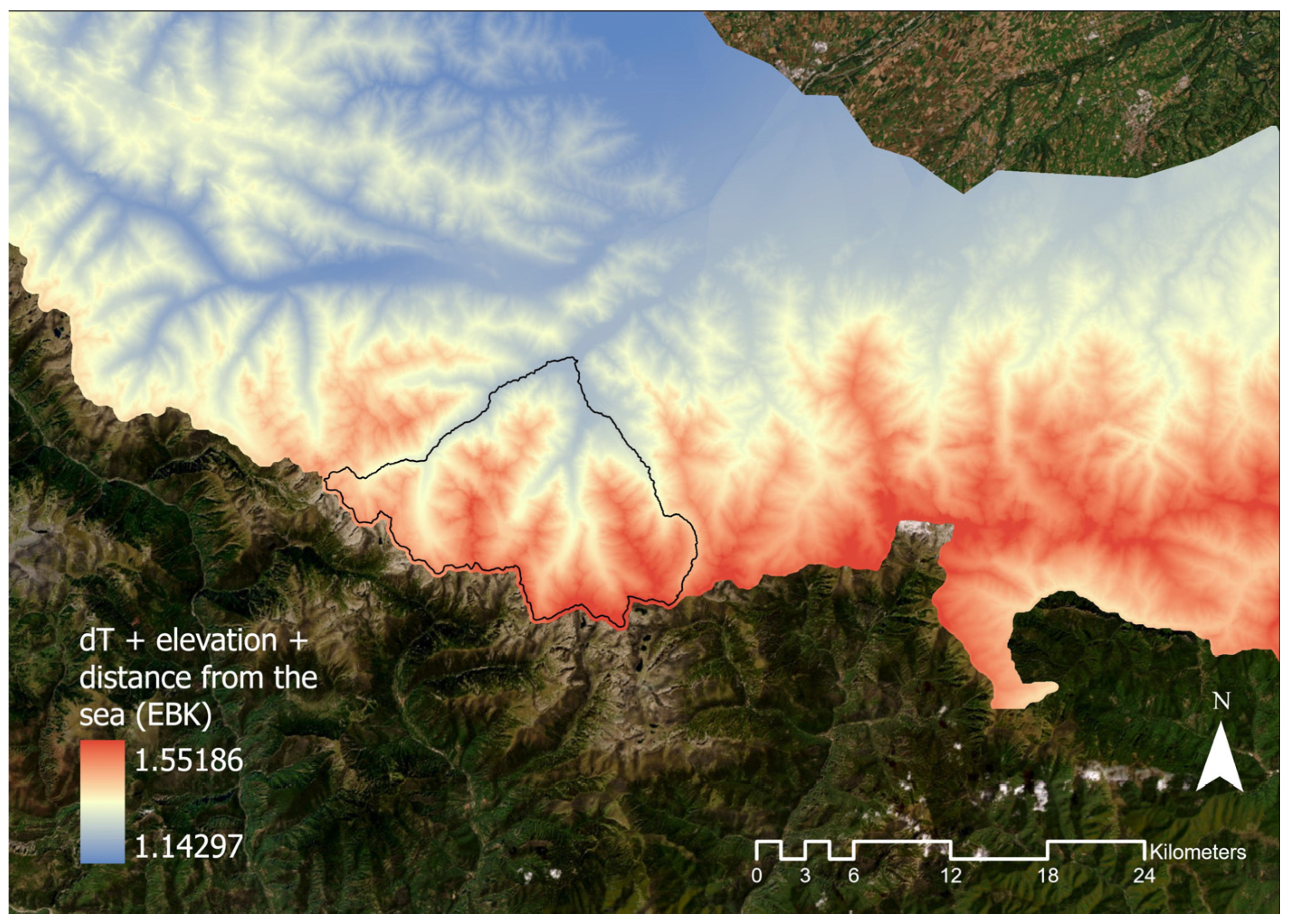
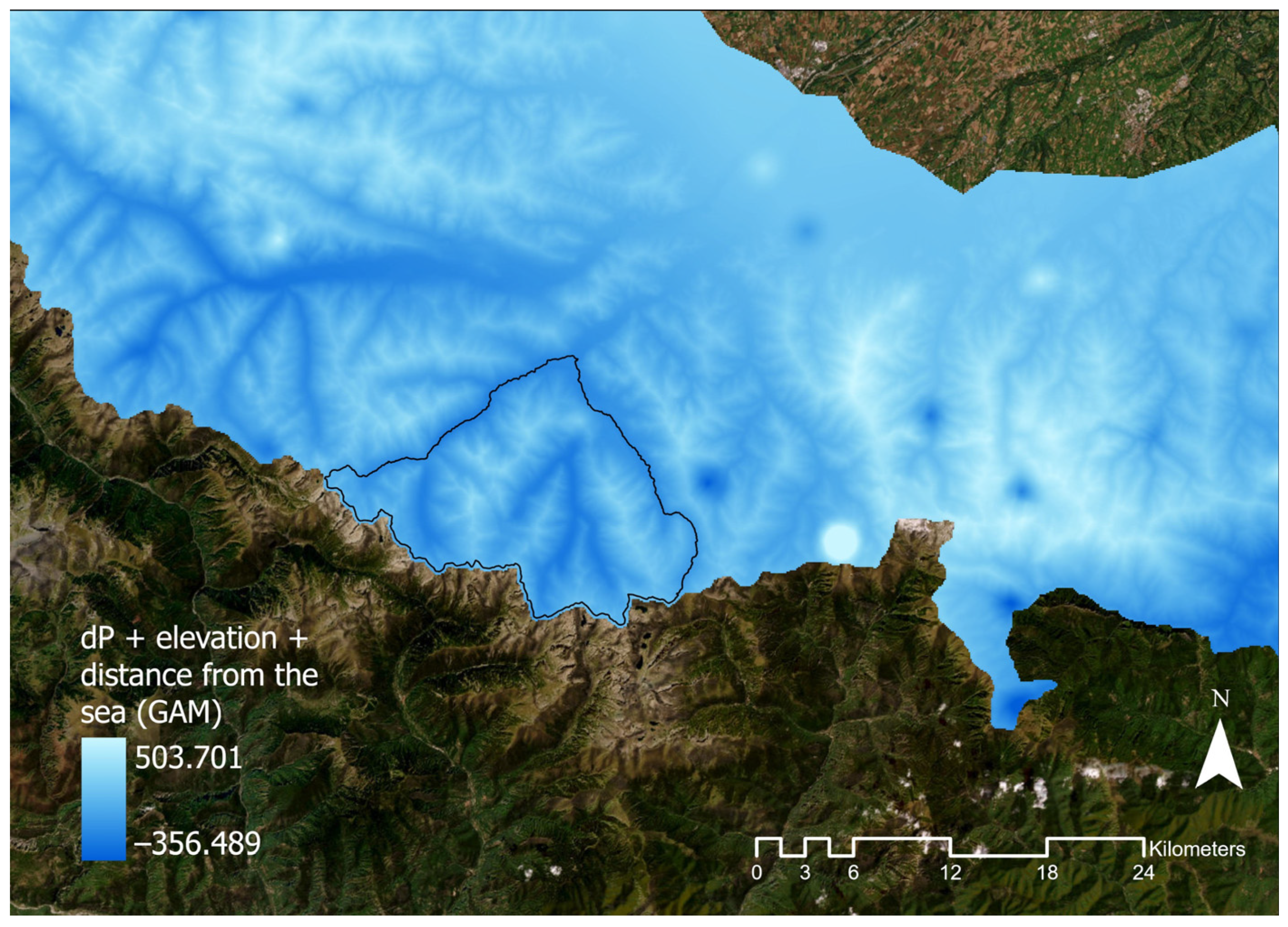
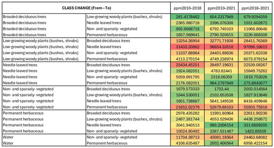
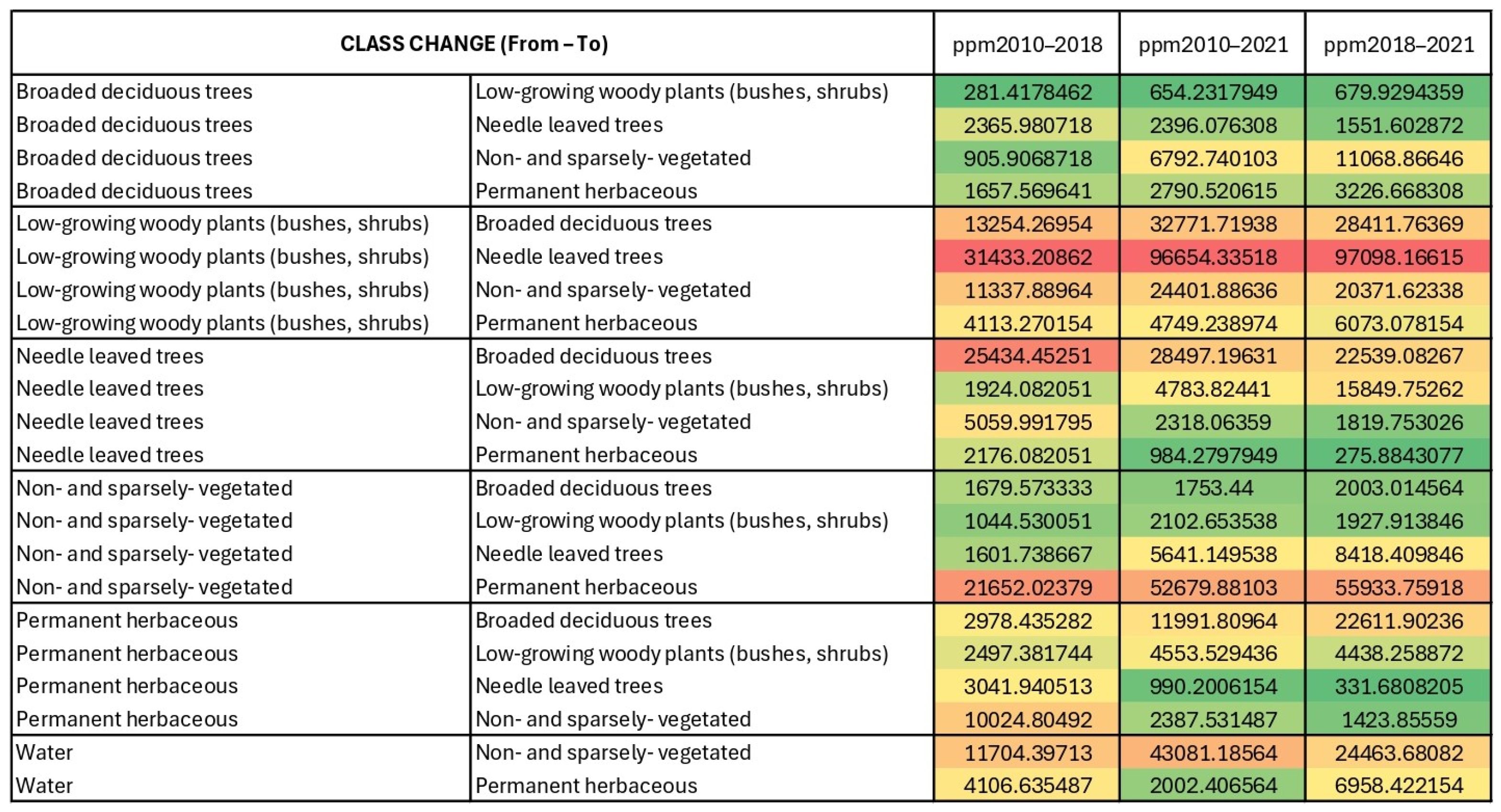
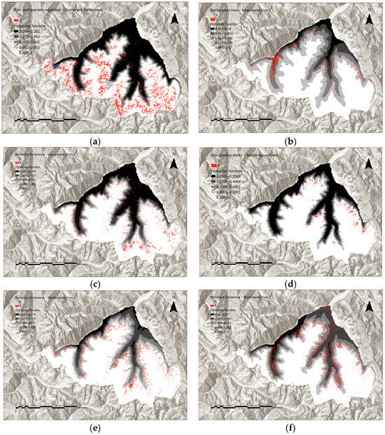
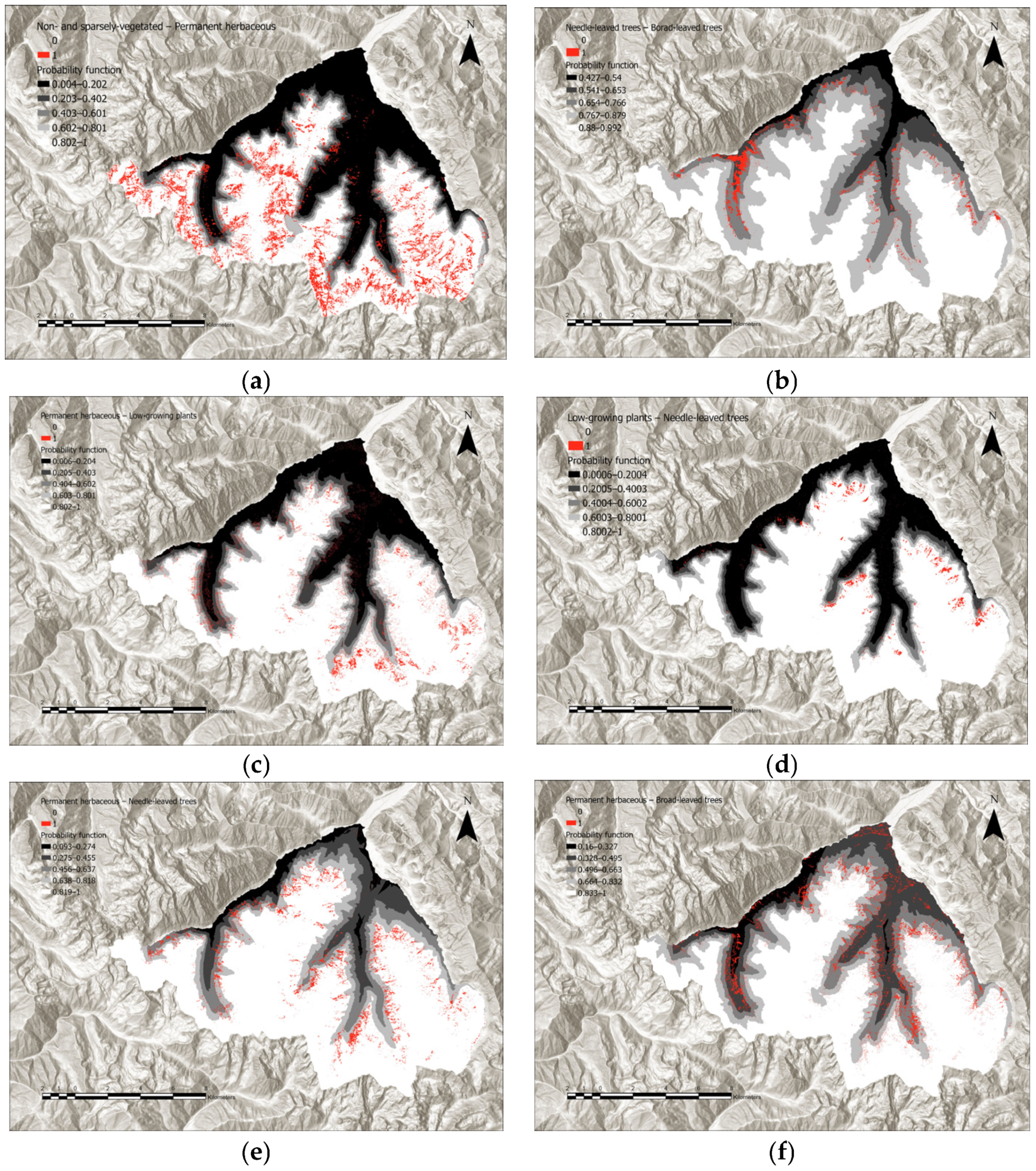

Disclaimer/Publisher’s Note: The statements, opinions and data contained in all publications are solely those of the individual author(s) and contributor(s) and not of MDPI and/or the editor(s). MDPI and/or the editor(s) disclaim responsibility for any injury to people or property resulting from any ideas, methods, instructions or products referred to in the content. |
© 2026 by the authors. Licensee MDPI, Basel, Switzerland. This article is an open access article distributed under the terms and conditions of the Creative Commons Attribution (CC BY) license.