Climate Variability-Induced Rainfall Trends in the Baitarani River Basin, India: A Spatio-Temporal and GIS-Based Assessment

Abstract

Understanding spatio-temporal rainfall variability is critical for water resource management, especially for climate-sensitive river basins. This study examines rainfall trends and variability in the Baitarani River Basin (eastern India) using high-resolution gridded data for 1979–2020. Rainfall trends were investigated using non-parametric Mann–Kendall test (MK test) and Sen’s slope estimator (SSE). The shift point was detected using multiple homogeneity tests [Pettitt test, Standard Normal Homogeneity Test (SNHT), and Buishand test], while rainfall variability was quantified using an entropy-based Marginal Disorder Index (MDI). The analyses were performed at annual and seasonal scales. MK Z-statistic indicates the increasing or decreasing nature of a series, whereas Sen’s β slope provides the rate of change in that particular series. The MK test and SSE were applied again to examine trends before and after the identified change point. Finally, maps illustrating spatial trends and percentage changes were produced using ArcGIS 10.6. Over the 42-year period, the MK test revealed significant increasing annual trends in both districts, Keonjhar (Z = +2.4, β = 0.7 mm/year), with a percentage change of around +21.8%, and Mayurbhunj (Z = +2.4, β = 0.7 mm/year), with a percentage change of around +19.2%. During 1979–2020 post-monsoon rainfall showed the highest increase (62–70%) while, post 2001, monsoon rainfall declined substantially (1.7–3.3 mm/year) across all districts, with Balasore showing the largest decrease (−3.3 mm/year). The earlier period (1979–2001) had stable monsoon rainfall but greater variability in retreating monsoon, especially in northern regions. Entropy-based variability analysis indicated the Bhadrak and Balasore districts as having maximum variability with an MDI value of 1.44 and 1.35, respectively, for monsoon and annual rainfall series. These findings underscore the importance of incorporating changing seasonal dynamics into water-resource planning and flood-risk management for the Baitarani River Basin in the context of climate change.

1. Introduction

Large-scale changes in socio-economic systems world-wide are driving the climatic change and global warming. Climatic variability is characterized by changes in precipitation, temperature, wind velocity, evaporation, humidity, and other meteorological parameters across temporal scales. Climate variability within a region is reflected through both gradual trends and abrupt changes in meteorological parameters such as precipitation [1]. Precipitation variability differs across regions and climatic conditions, with rainfall trends showing increasing, decreasing, or stable behavior over time. A visible variability in global precipitation pattern is seen across all climatic scenarios [2]. Rainfall is a key hydrological variable that strongly influences water availability, as changes in its magnitude and spatial–temporal distribution directly affect surface water resources, groundwater recharge, and water supply systems. The hydrologists and researchers, nowadays, are more concerned about the changing rainfall patterns due to climate change [3,4]. The identification, assessment, and prediction of rainfall trends and their impacts on the basin water availability pose considerable challenges in the context of climate change [5]. The analysis of rainfall trend helps in forecasting rainfall, reservoir operations, planning water resources, optimizing irrigation, and quantifying the amount of flow in a river basin [6]. Furthermore, rainfall data serves as a critical input for supporting industrial development, strengthening water supply systems, and guiding climate disaster management strategies in both present and future contexts [7]. In monsoon-dependent agricultural regions of eastern India, variations in rainfall significantly affect agricultural productivity and water availability. Climate variability and changing monsoon patterns significantly influence hydrology, agriculture, and water resources in many parts of India. Since agricultural productivity largely depends on seasonal rainfall, long-term analysis of rainfall variability is essential for understanding regional water availability, crop planning, and flood–drought risks [8]. Variations in precipitation and extreme rainfall events can adversely affect agriculture, food security, and the broader economy [9].

The spatio-temporal distribution of precipitation in India is highly erratic. Runoff generated from this precipitation significantly influences sustainable agricultural practices and meets water supply requirements, both from surface water and groundwater [10]. The domestic water demand from a substantial population leads to water-stressed conditions throughout India, particularly during the summer months. Notably, nearly 80% of the country’s annual precipitation is concentrated in the four months of monsoon season, which typically spans from June to September [11]. Several studies have investigated long-term rainfall trends in India and other regions, reporting both increasing and decreasing precipitation patterns [12,13,14]. For example, Kumar et al. [15] analyzed monthly and seasonal rainfall trends across 30 meteorological subdivisions of India using data from 1871 to 2005 and observed significant regional variability in rainfall trends. The study found that nearly half of these sub-divisions showed an increasing annual rainfall trend, particularly in regions such as Haryana, Punjab, and Coastal Karnataka, except the Chhattisgarh sub-division, which displayed a statistically significant decreasing trend. In the southwest monsoon period, Jharkhand, Chhattisgarh, and Kerala showed clear decreasing rainfall trends. In contrast, Gangetic West Bengal, West Uttar Pradesh, Jammu and Kashmir, Konkan and Goa, Madhya Pradesh, Rayalseema, Coastal Andhra Pradesh, and North Interior Karnataka experienced significant increasing precipitation trends [16]. An analysis of monthly, seasonal, and annual rainfall data in Kerala from 1871 to 2005 revealed a significant decline in southwest monsoon rainfall and an increase in post-monsoon precipitation, while winter and summer rainfall showed statistically insignificant increasing trends [17].

Basin-scale studies on land use, soil erosion, flooding, and streamflow variability in the Baitarani River Basin confirm that climatic factors such as changes in temperature and monsoon rainfall patterns are primary drivers of recent hydrological change [18,19,20,21]. Observational studies in the sub-basin report a slight increase in annual rainfall alongside considerable interannual variability, producing both wetter periods and prolonged dry spells [22]. Increasing extreme rainfall events and stronger monsoon activity in Odisha have further contributed to higher runoff and flood frequency [23]. Climate projections for the Brahmani–Baitarani system suggest future intensification of rainfall and extreme precipitation, with compounding risks for flooding and erosion [24].

In addition to hydrological impacts, climate variability also affects water quality and groundwater conditions [25,26,27,28,29]. Increasing flood and drought occurrences may reduce agricultural water availability and increase environmental stress within the basin. Therefore, improved forecasting systems, watershed management, and adaptive water-resource planning are important for reducing climate-related vulnerability [30]. Recent studies on the Baitarani River Basin indicate noticeable hydro-climatic variability, including changes in rainfall distribution, seasonal fluctuations, and variability in runoff generation and basin hydrology [31]. Variations in precipitation and temperature have also been reported to influence the basin water balance, highlighting the sensitivity of the region to climatic variability and change [32].

Monsoon-dependent river basins such as the Baitarani River are among the most hydrologically sensitive systems worldwide, yet comprehensive basin-scale investigations that integrate trend analysis, homogeneity assessment, and entropy-based variability evaluation remain limited, especially in eastern India. Consequently, understanding long-term rainfall variability is crucial for sustainable water-resource planning and agricultural management within these basins. This study addresses this research gap by going beyond simple rainfall trend detection to interpret the underlying hydro-climatic drivers and their implications for water resources. The analysis employs the Mann–Kendall test and Sen’s Slope Estimator for trend detection, multiple homogeneity tests for identifying shift points, and the entropy-based Marginal Disorder Index (MDI) to quantify variability at both annual and seasonal scales. The proposed integrated multi-method framework is readily applicable to other monsoon-dependent basins across South and Southeast Asia. Furthermore, the identification of temporal shifts in seasonal rainfall distribution provides valuable insights for reservoir management, groundwater recharge planning, flood-risk mitigation, and agricultural scheduling in monsoon-influenced regions globally.

2. Materials and Methods

2.1. Study Area

The Baitarani River Basin is located in eastern India, primarily within the state of Odisha. The Baitarani River Basin is characterized by predominantly alluvial and lateritic soils and includes hilly uplands, plateaus, and plains. The basin receives an average annual rainfall of approximately 1200–1600 mm, of which nearly 75–85% occurs during the southwest monsoon season (June–September). The deltaic regions are highly fertile and are mainly cultivated with paddy as the dominant crop. Other crops such as pulses, oilseeds, vegetables, and millets are also grown in different seasons. The basin also has considerable potential for crop diversification and improved irrigation practices.

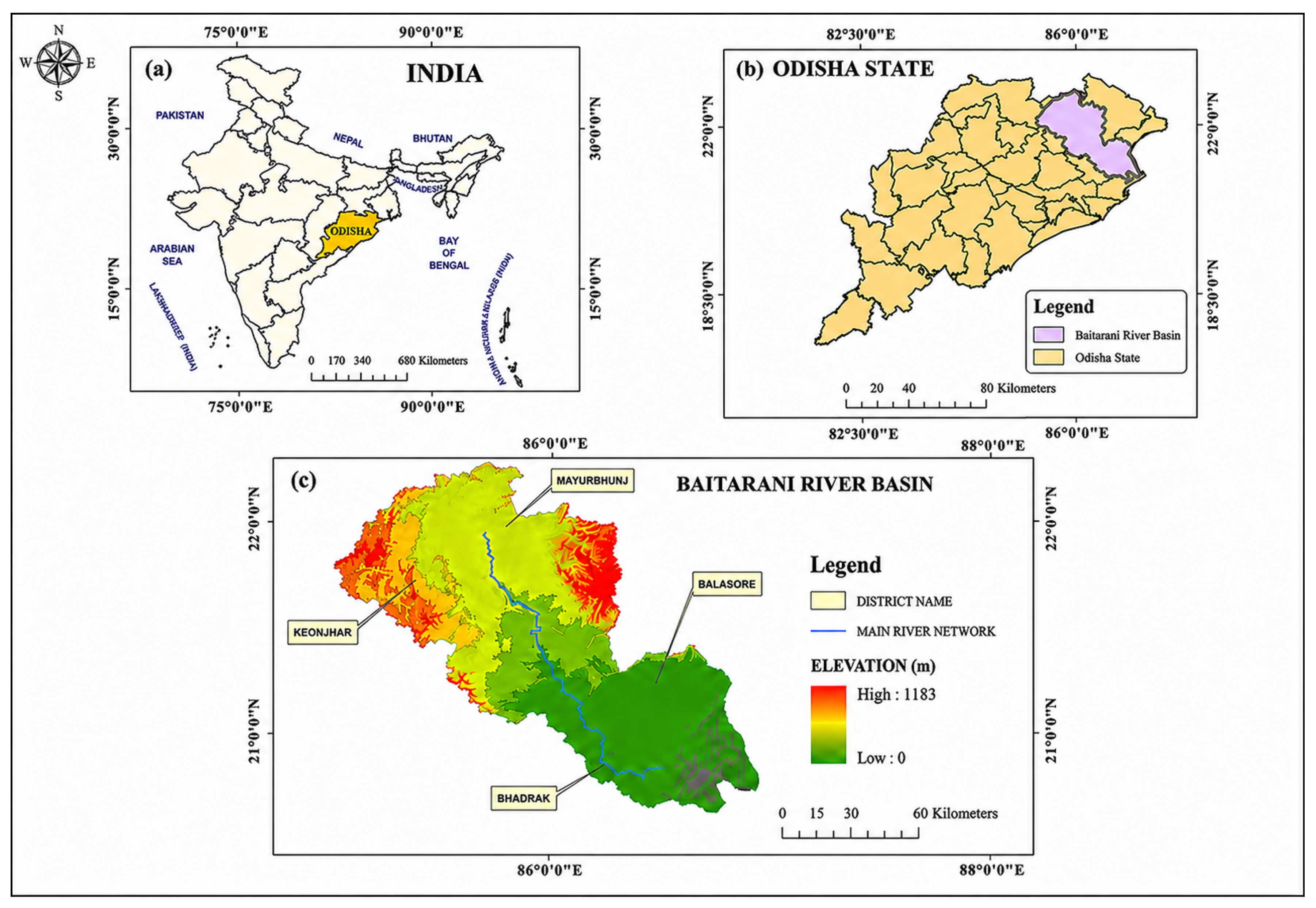
Temperature varies seasonally across the basin. Summer temperatures generally range from 35 °C to 40 °C, while winter temperatures decrease to about 12–15 °C. The average annual temperature remains between 25 °C and 27 °C, indicating a warm tropical climate. These hydro-climatic conditions strongly influence agricultural practices and cropping patterns. However, the heavy dependence on monsoon rainfall makes agriculture vulnerable to rainfall variability and prolonged dry spells. Therefore, efficient irrigation scheduling, rainwater harvesting, and conjunctive use of surface water and groundwater resources are important for improving agricultural productivity (Figure 1).

Table 1. General statistics of annual and seasonal rainfall (mm) for different districts in and around Baitarani River Basin.

Statistics	Districts				Baitarani River Basin
	Keonjhar	Mayurbhunj	Balasore	Bhadrak	Whole Basin	Pre-Monsoon	Monsoon	Post Monsoon	Winter
Mean ± SD	1692 ± 235	1750 ± 243	2061 ± 249	1673 ± 318	1794 ± 247	227 ± 86	1412 ± 216	117 ± 69	37 ± 26
CV	0.14	0.14	0.15	0.15	0.14	0.38	0.15	0.59	0.71
Kurtosis	−0.61	−0.58	0.2	0.34	−0.41	1.3	−0.31	0.42	−0.13
Skewness	−0.1	−0.03	−0.12	0.16	−0.21	0.94	0.23	1.05	0.53
Minimum	1215	1278	1361	1124	1245	70	1034	30	2
Maximum	2108	2185	2847	2258	2299	484	1947	303	108
Median	1700	1735	2085	1675	1818	213	1419	104	37

shows annual rainfall statistics of four districts in and around the Baitarani River Basin. Keonjhar, Mayurbhunj, Balasore, Bhadrak and the basin itself receive average annual rainfall ranging from about 1673 mm to 2061 mm. The rainfall amounts are moderately consistent, as seen from the low variation and standard deviation values.

The seasonal rainfall statistics for the Baitarani River Basin based on district-wise gridded rainfall data extracted from the India Meteorological Department (IMD) dataset for Keonjhar, Mayurbhunj, Balasore, and Bhadrak districts. The results show that most of the annual rainfall (approximately 1412 mm) occurs during the southwest monsoon season (June–September), while pre-monsoon, post-monsoon, and winter seasons contribute comparatively lower rainfall amounts. The coefficient of variation is higher during pre-monsoon, post-monsoon, and winter seasons, indicating greater seasonal variability in rainfall compared to the monsoon period.

2.2. Data Description

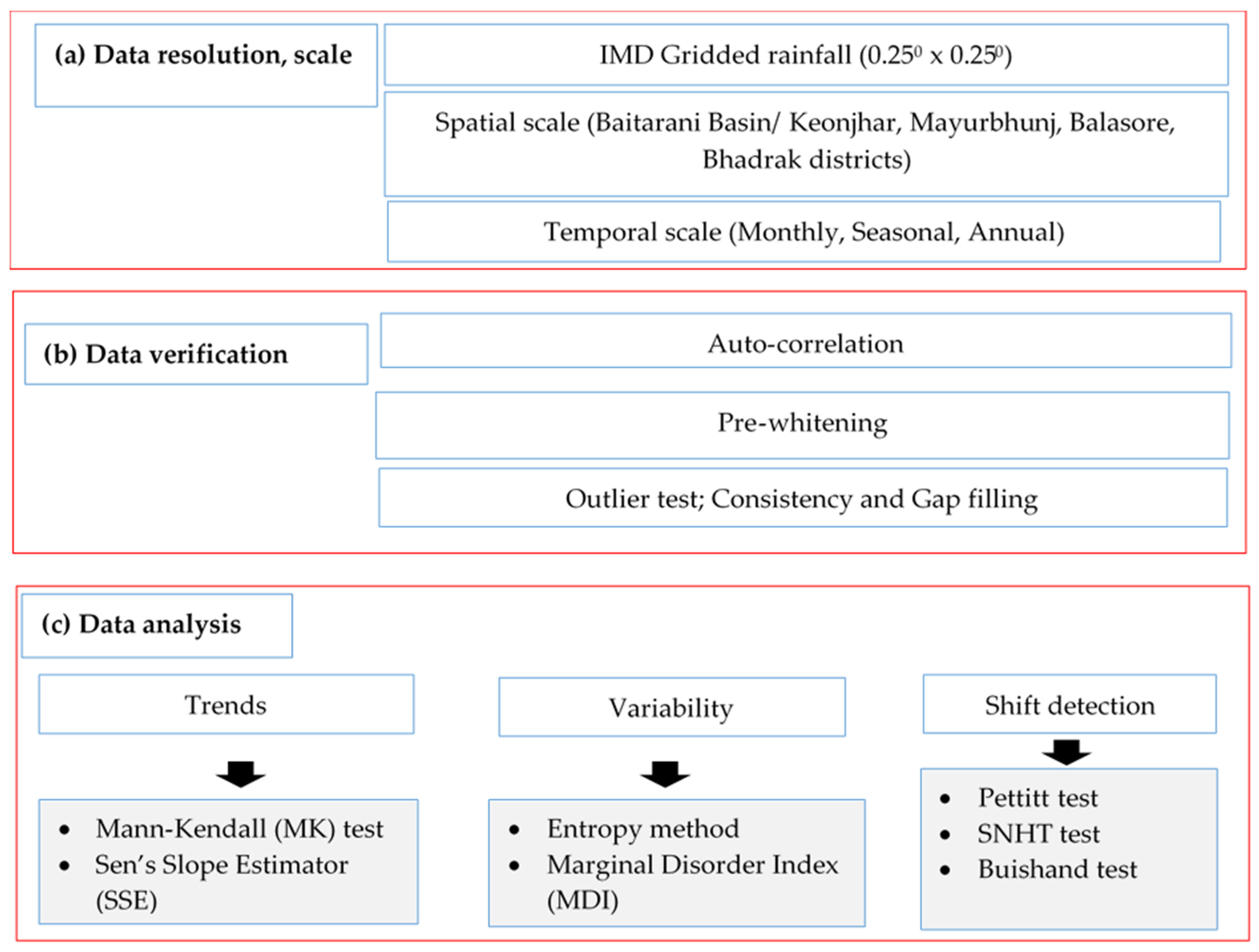
In this study, high-resolution daily gridded rainfall data for the period 1979–2020 were obtained from the IMD database. The study period of 1979–2020 spans 42 years, substantially exceeding the 30-year climatological normal period recommended by the World Meteorological Organization (WMO), as the standard reference baseline for climate analysis. This record length of 42 years is considered adequate for detecting statistically meaningful trends and change points in hydro-climatic variables. This dataset provides rainfall estimates around 0.25 degree × 0.25 degree resolution (27.5 km into 27.5 km), developed by interpolating rainfall observations for more than 6995 rain gauge stations across India using the Shepherd’s Interpolation Method. The rainfall dataset was checked for outliers before applying the non-parametric Mann–Kendall trend test [33]. Rainfall datasets frequently show non-normal distributions, making non-parametric methods suitable for trend analysis. The magnitude of change over time was then estimated using Sen’s slope estimator [34]. Pettitt, SNHT, and Buishand homogeneity tests were applied to detect possible change points in the rainfall series. The analyses generally indicated a shift around the year 2001. The data were then grouped in two periods, i.e., before shift (1979–2001) and after shift (2002–2020). The Mann–Kendall test and Sen’s slope estimator were then applied separately to each period to compare trend characteristics before and after the detected change point. Since the Mann–Kendall test assumes data independence, autocorrelation in the rainfall series was assessed prior to trend analysis to ensure the reliability of the statistical results. It is noted that the post-shift sub-period (2002–2020, n = 19) has a reduced sample size compared to the full record (n = 42). The reduced sample size lowers the statistical power of the MK test, meaning that genuine trends of moderate magnitude may not achieve statistical significance. In addition to trend analysis, an entropy-based Marginal Disorder Index (MDI) method [35] was applied to quantify the variability and irregularity of rainfall distribution across different temporal scales. Higher entropy values indicate greater uncertainty and variability in rainfall occurrence, whereas lower values represent relatively uniform rainfall behavior. This approach complemented the trend analysis by identifying periods with greater rainfall variability that may not be fully captured through monotonic trend detection alone. The spatial distribution of rainfall variability, homogeneity, and trend patterns was mapped in ArcGIS 10.6 using the Inverse Distance Weighting (IDW) interpolation technique. IDW interpolation was performed using a power parameter of two and the nearest neighboring grid points to estimate spatial variation across the basin. The interpolation results were visually examined and compared with observed rainfall characteristics to ensure consistency in spatial representation. The overall methodology adopted in this study is illustrated in Figure 2.

2.2.1. Outlier Test

Outliers are values that are noticeably different from the overall pattern of a data set. Including these values in analysis can affect the results, especially when the sample size is small, as they may distort key statistical measures [36]. Outlier analysis was performed on the rainfall dataset, and no abnormal values requiring removal were identified. The Water Resources Council, 1981 approach was used as a preliminary quality-control method for identifying potential outliers in the rainfall dataset, as it remains commonly applied in hydro-climatic studies involving moderately skewed data using the following equations before deciding whether to remove them:

$$Y_H=\overline{y}+K_n{S}_y\hspace{1em}(\mathrm{High} \mathrm{outliers})$$

(1)

$$Y_L=\overline{y}-K_n{S}_y\hspace{1em}(\mathrm{Low} \mathrm{outliers})$$

(2)

Here the high outlier threshold (Y_H) is expressed in logarithmic units. The mean ($\overline{y}$) and standard deviation (S_y) are also calculated in log units. The constant (K_n) depends on the sample size (n). The low outlier threshold (Y_L) is likewise defined in log units. For sample sizes of 32 and 40, the corresponding K_n values are 2.682 and 2.591, respectively.

2.2.2. Auto Correlation Test

Since the Mann–Kendall test assumes independent observations, lag-1 autocorrelation was evaluated before trend analysis. Where significant autocorrelation was detected, pre-whitening was applied prior to the MK test. The existence of either positive or negative autocorrelation significantly influences the trend observed within a given series [37]. Lag-1 autocorrelation analysis was performed to evaluate serial dependence in the rainfall time series before applying trend analysis. When the time series shows random behavior or when the lag-1 serial correlation is not statistically significant, the MK test is applied directly to the original data. However, if significant serial correlation is present in the time series, the modified Mann–Kendall (MMK) test is used after removing the effect of serial correlation [38,39]. The autocorrelation coefficient rk at lag k for a discrete time series is calculated using the following expression:

$${\mathrm{r}}_{\mathrm{k}}={\displaystyle \frac{{\displaystyle {\sum }_{\mathrm{k}=1}^{\mathrm{n}-\mathrm{k}}}({\mathrm{X}}_{\mathrm{t}}-{\overline{\mathrm{X}}}_{\mathrm{t}})({\mathrm{X}}_{\mathrm{t}+\mathrm{k}}-\overline{{\mathrm{X}}_{\mathrm{t}+\mathrm{k}}})}{[{\displaystyle {\sum }_{\mathrm{k}=1}^{\mathrm{n}-\mathrm{k}}}{\left({\mathrm{X}}_{\mathrm{t}}-{\overline{\mathrm{X}}}_{\mathrm{t}}\right)}^2{\left({{\mathrm{X}}_{\mathrm{t}+\mathrm{k}}-\overline{{\mathrm{X}}_{\mathrm{t}+\mathrm{k}})}}^2\right]}^{0.5}}}$$

(3)

Here, r_k = autocorrelation coefficient at lag k, X_t = rainfall value at time step t, X_t+k = rainfall value at lag k,$\overline{X}$= mean of the rainfall series, and n = total number of observations. To evaluate serial independence in the rainfall time series, the lag-1 autocorrelation coefficient (r₁) was examined. The null hypothesis assumes that the series has no serial correlation (H₀:r₁ = 0), whereas the alternative hypothesis indicates the presence of serial correlation (H₁:r₁≠0). This is evaluated using the significance test for serial correlation, described as:

$${(r_k)}_{t_g}={\displaystyle \frac{-1\pm t_g{(n-k-1)}^{1/2}}{n-k}}$$

(4)

In this case, (r_k)_tg represents the normally distributed value of the autocorrelation coefficient r_k, and t_g denotes the critical value of the normal distribution at a given significance level g. The critical values of the standardized test statistic (t_g) are 1.645, 1.96, and 2.326 at the 10%, 5%, and 1% significance levels, respectively, based on the standard normal distribution for a two-tailed test as described in equation (4). When the absolute value of r_k is greater than or equal to (r_k)_tg, the null hypothesis of serial independence is rejected at the chosen significance level α (0.05 in this study). For datasets that do not follow a normal distribution, the MK test is considered suitable for trend detection. To ensure the validity of the Mann–Kendall (MK) test, lag-1 autocorrelation was first evaluated for each rainfall time series. When significant autocorrelation was absent, the MK test was applied directly. In cases where significant autocorrelation was detected, pre-whitening was performed prior to trend analysis to minimize the influence of serial correlation.

2.2.3. Pre-Whitening

Pre-whitening was applied to rainfall series exhibiting significant lag-1 autocorrelation in order to reduce the influence of serial dependence prior to Mann–Kendall trend analysis. This procedure helps minimize the possibility of detecting spurious trends caused by autocorrelation rather than actual temporal changes in the rainfall series [40]. The series may be subjected to pre-whitening through the application of the following formula:

$$Y_t\hspace{0.17em}=\hspace{0.17em}{Y}_i-r_k{X}_{i-1}$$

(5)

where Y_t = pre-whitened rainfall value at time step t, Y_i = original rainfall observation at time step t, X_i−1 = rainfall observation at the previous time step, and r_k = lag-k autocorrelation coefficient (commonly lag-1 autocorrelation in pre-whitening applications). Pre-whitening was performed only for rainfall series exhibiting statistically significant autocorrelation, as the requirement depends on dataset characteristics rather than fixed coefficient of variation or sample-size criteria.

2.3. Data Processing and Analysis

2.3.1. Mann–Kendall (MK) Test for Identifying Trends

In this study, the non-parametric Mann–Kendall (MK) test was applied to detect monotonic trends in annual, seasonal, and monthly rainfall series of the Baitarani River Basin. The method was selected because it is suitable for hydro-climatic datasets that may contain non-normal distributions and data gaps [41]. The MK test statistic, denoted as S, is calculated as follows:

$$\mathrm{S} = {\displaystyle {\sum }_{i=1}^{n-1}}{\displaystyle {\sum }_{j=i+1}^n}sgn(x_j-x_i)$$

(6)

Here, x₁, x₂, x₃,…x_n refers to the individual data values n in the time series where x_j refers to the point data at time j of time series data and x_i represents the rainfall value at time step i and x_j-x_i = θ

$$Sgn\left(\theta \right)=\left\{\begin{array}{c}1 if \theta >0\\ 0 if \theta =0\\ -1 if \theta <0\end{array}\right.$$

(7)

The statistics S follows an approximate normal distribution when n ≥ 10, which is sufficiently large, with its mean and variance defined as follows:

$$E\left[S\right]=0$$

(8)

$$Var\left(S\right)={\displaystyle \frac{n\left(n-1\right)\left(2n+5\right)-{\displaystyle {\sum }_{i=1}^n}{t}_i\left(t_i-1\right)(2t_i+5)}{18}}$$

(9)

Here t_i denotes the number of tied groups of size I. The standardized test statistic (z) of the Mann–Kendall (MK) test and the associated one-tailed p-value (p) are calculated using the following expressions:

$$Z=\left\{\begin{array}{c}{\displaystyle \frac{S-1}{\sqrt{Var\left(S\right)}}} if S>0\\ 0 if S=0\\ {\displaystyle \frac{S+1}{\sqrt{Var\left(S\right)}}} if S<0\end{array}\right.$$

(10)

$$p=2[1-\varnothing \left(\left|Z\right|\right)]$$

(11)

where p = two-tailed p-value, Z = standardized Mann–Kendall test statistic, and Φ(∣Z∣) = cumulative distribution function (CDF) of the standard normal distribution evaluated at ∣Z∣.

$$\varphi \left(\left|Z\right|\right)\hspace{0.17em}=\hspace{0.17em}{\displaystyle \frac{1}{\sqrt{2\pi }}}\hspace{0.17em}{\displaystyle {\displaystyle \underset{0}{\overset{\left|Z\right|}{\int }}}{e}^{-\hspace{0.17em}\hspace{0.17em}\frac{t^2}{2}}dt}$$

(12)

Positive and negative Z values indicate increasing and decreasing trends, respectively. At the 5% significance level, the null hypothesis of no trend is rejected when the absolute value of the standardized test statistic exceeds the critical value (∣Z∣ > 1.96), corresponding to p < 0.05 for a two-sided test.

2.3.2. Trend Estimation by Theil–Sen’s Estimator (Sen’s Slope Estimator) Test

When a time series exhibits a linear trend, the magnitude of change can be estimated using Sen’s slope estimator proposed by Sen (1968) [42]. The method determines the slope by calculating pairwise changes between observations in the time series. It is computed by:

$$T_{jk}={\displaystyle \frac{x_j-x_k}{j-k}}for \mathrm{all} j>k$$

(13)

In this expression, $x_j$ and $x_k$ denotes the data values observed at times j and k (j > k). Sen’s slope is estimated as the median of all pairwise slope values (Tjk) calculated from the data series.

$$\beta =\left\{\begin{array}{c}{\displaystyle \frac{T_{N+1}}{2}} , N is odd\\ {\displaystyle \frac{1}{2}}\left(T_{{\displaystyle \frac{N}{2}}}+T_{{\displaystyle \frac{N+2}{2}}}\right),N is even\end{array}\right.$$

(14)

A positive value $\beta$ shows that the time series is increasing overtime, whereas a negative value shows a decreasing trend.

2.3.3. Percentage Change

Percentage change between two time series was estimated using a linear trend approach based on Sen’s slope estimator. Percentage change is computed by approximating it with a linear trend.

$$Percentage Change \left(\%\right)={\displaystyle \frac{\beta (Length of year)}{Mean}}\times 100$$

(15)

2.4. Homogeneity Test

2.4.1. Pettitt Test

Pettitt test is a non-parametric method used to detect change points in a time series [43]. Based on the Mann–Whitney test, it identifies the point at which a significant shift occurs in the data series. For a time series (X₁, X₂,…,Xn) of length n, let t represent the most probable time of change. The series is then divided into two groups (X₁, X₂,…,X_t) and (X_t+1,X_t+2,…,X_n). Test statistic, U_t, is calculated following the method proposed in [43]:

$$U_t={\displaystyle {\sum }_{i=1}^t}{\displaystyle {\sum }_{j=1}^T}sgn(X_i-X_j)$$

(16)

where

$$sgn\left(x_j-x_i\right)=\left\{\begin{array}{c}1, if\left(x_j-x_i\right)>0\\ 0, if\left(x_j-x_i\right)=0\\ -1, if\left(x_j-x_i\right)<0\end{array}\right.$$

(17)

In Pettitt test, a change point is identified at the location where the test statistic Ut reaches its maximum absolute value, indicating a significant shift in the time series. Therefore, it becomes necessary to identify the most important change point. The most significant change point t is determined at the time when the value of |U_t| reaches its maximum.

$$K_T=\underset{1\le t\le T}{\max }\left|U_t\right|$$

(18)

Here, the estimated significance probability p(t) associated with a change point is calculated using the approach proposed by Pettitt (1979):

$$p=1-exp\left[{\displaystyle \frac{{-6K}_T^2}{T^3+T^2}}\right]$$

(19)

A change point of time t is considered statistically significant at the significance level α when the probability p(t) is smaller than (1-α).

2.4.2. Standard Normal Homogeneity (SNHT) Test

The SNHT was introduced by Alexandersson & Moberg (1986) [44] to detect change in time series data. In this test, the time series is split into two parts, the first part from 1 to t years (Z₁) and the second part from t to n–t years (Z₂). The test statistic (T_t) was calculated by comparing the two series using the mathematical Equations (20)–(22)

$$Tt=t{z}_1^2+(n-t)z_2^2$$

(20)

Z₁ and Z₂ were computed using the following formula:

$$Z_1={\displaystyle \frac{1}{t}}{\displaystyle {\sum }_{i=1}^t}{\displaystyle \frac{(x_i-\overline{x})}{\sigma x}}$$

(21)

$$Z_2={\displaystyle \frac{1}{(n-t)}}{\displaystyle {\sum }_{i=t+1}^n}{\displaystyle \frac{(x_i-\overline{x})}{\sigma x}}$$

(22)

In the above formula, $\overline{x}$ and $\sigma x$ represent the mean and standard deviation of the time-series data, respectively. The year t can be considered as a change point or breaking point where the value of T_t reaches its maximum value. The null hypothesis can be rejected when the statistic value is higher than the critical value, which will depend on the sample size (n).

2.4.3. Buishand Test

Buishand test [45] is commonly applied for detecting shifts in hydro-climatic time series and is generally robust for practical applications, although its statistical performance has been most extensively evaluated for approximately normally distributed data. The test is generally used in a two-tailed form, though one-tailed testing is also possible when using the Q statistic. In addition, Buishand introduced another statistic, R, which is designed only for two-sided hypothesis testing.

For the Q statistic, the null hypothesis assumes that the rainfall series is homogeneous and that no significant change point exists in the mean of the series. The alternative hypothesis indicates the presence of a significant shift in the mean at a certain point in time. The computation of the test statistic proceeds as follows (Equation (23)):

$$B_t={\displaystyle {\sum }_{i=1}^t}(x_i-\overline{x})$$

(23)

A time series without any change point may be considered homogeneous if the B_t statistic is approximately equal to zero. This is because a time series with a random distribution around its mean value will exhibit this behavior on both sides of the mean series. The presence of a significant shift in the series can be evaluated by (Equation (24) the rescaled adjusted range (R)

$$R={\displaystyle \frac{Max\left(B_t\right)-Min\left(B_t\right)}{\overline{x}}}$$

(24)

2.4.4. Moving Average

A 3-year moving average was applied to smooth short-term fluctuations in the rainfall series and to better visualize long-term variability and trend patterns. The selected window size was considered appropriate for reducing interannual variability while preserving the overall temporal behavior of rainfall. This window length is consistent with prior studies on Indian basin-scale rainfall variability [5,7]. Longer windows (≥5 years) would obscure the transition behavior around the 2001 shift point and reduce the effective sample size for sub-period interpretation.

2.5. Entropy Method

Initially developed by Shannon [37] for communication theory, the entropy method is now widely applied in hydrology and water resource management studies. This methodology fundamentally addresses the uncertainty level associated with various datasets. Entropy quantifies the degree of randomness inherent in the outcomes of stochastic processes such as rainfall. Entropy can be expressed in several forms, including marginal entropy, conditional entropy joint entropy, and transformational entropy. Shannon [37] introduced a discrete expression for entropy, which is presented below

$$H\left(X\right)=-{\sum }_{i=1}^{N}p\left(x_i\right)\log \left[p\left(x_i\right)\right]$$

(25)

Entropy H(X) represents the marginal entropy of the random variable X, where xi denotes the rainfall class and p(xi) represents its probability of occurrence. When the logarithm base is 2, entropy is expressed in bits. Entropy reaches its highest value when all possible events occur with nearly equal probability, indicating a uniform or unbiased distribution. On the other hand, entropy becomes zero when the occurrence of an event is completely certain. In such cases, there is no uncertainty in the system. Therefore, entropy values range from 0, representing minimum uncertainty, to log2 N, representing maximum uncertainty. In the present study, the Marginal Disorder Index (MDI) was used to evaluate rainfall variability across the basin during 1979–2020. Rainfall data were grouped into discrete classes based on rainfall magnitude intervals, and the probability of occurrence (pi) for each class was calculated from the relative frequency of observations within that class. These probabilities were then used to compute entropy and MDI values for assessing spatial and temporal rainfall variability. These class boundaries are consistent with those used by Mishra et al. [25] and permit straightforward comparison with other Indian basin studies.

2.6. Spatial Analysis of Time Series

To examine rainfall trends at annual and seasonal scales, the β coefficient was used instead of the traditional least squares method. This approach is preferred because it is less affected by non-normal data. Sen’s slope estimator was selected because it provides a robust measure of trend magnitude in hydro-climatic time series and is less sensitive to non-normal data and extreme values. The district-wise β slope values obtained from the rainfall series were spatially interpolated in ArcGIS 10.6 using the inverse distance weighted (IDW) method to visualize the spatial distribution of rainfall trends across the basin. A power parameter of two was used to assign greater influence to nearby observations, while the interpolation considered the nearest neighboring districts for surface estimation. The interpolated outputs were visually compared with observed spatial rainfall patterns to ensure spatial consistency across the basin [46]. In the study, IDW method was selected due to its simplicity, computational efficiency, and suitability for hydro-meteorological datasets with limited observation points. IDW assumes that nearby stations exert a greater influence on the interpolated values than distant stations, making it appropriate for representing regional rainfall variability and related climatic parameters.

3. Results

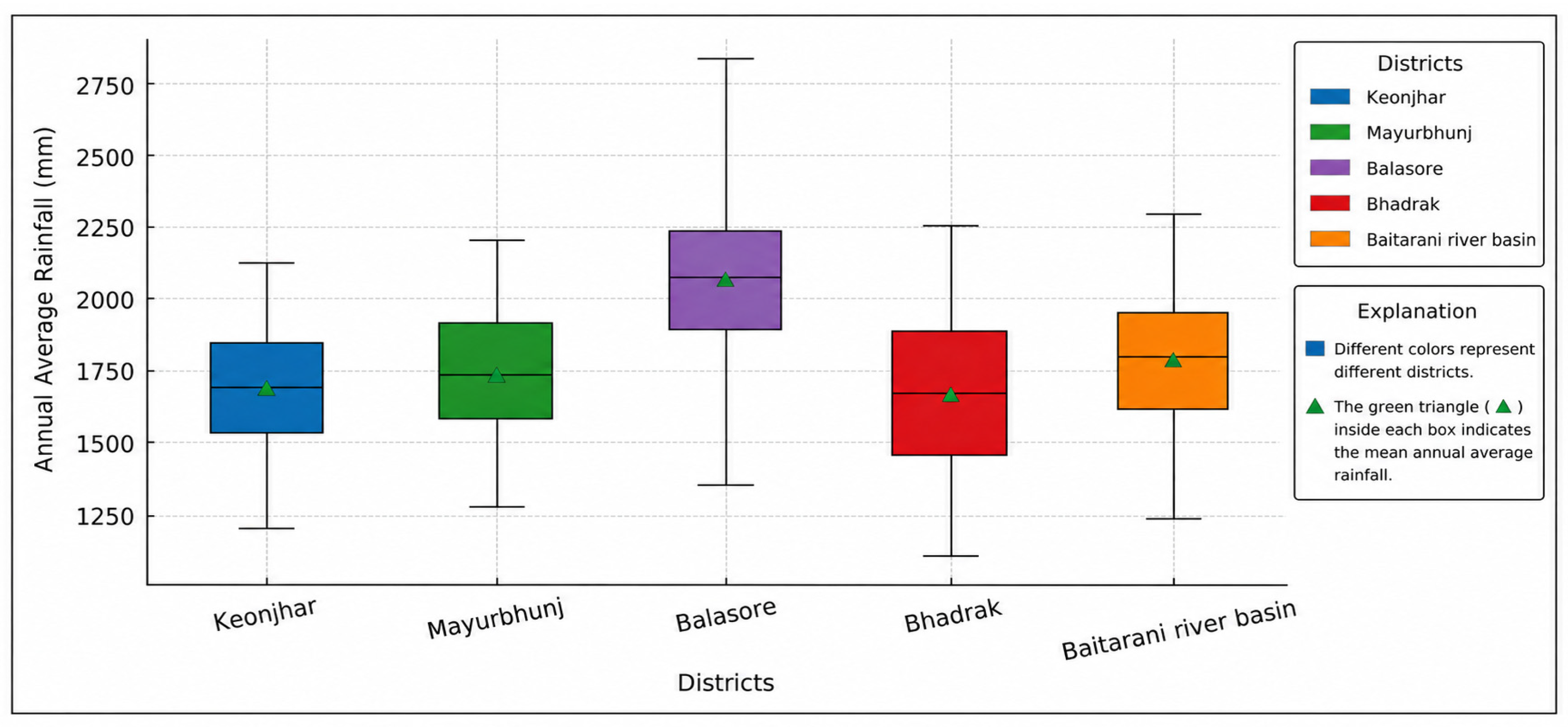
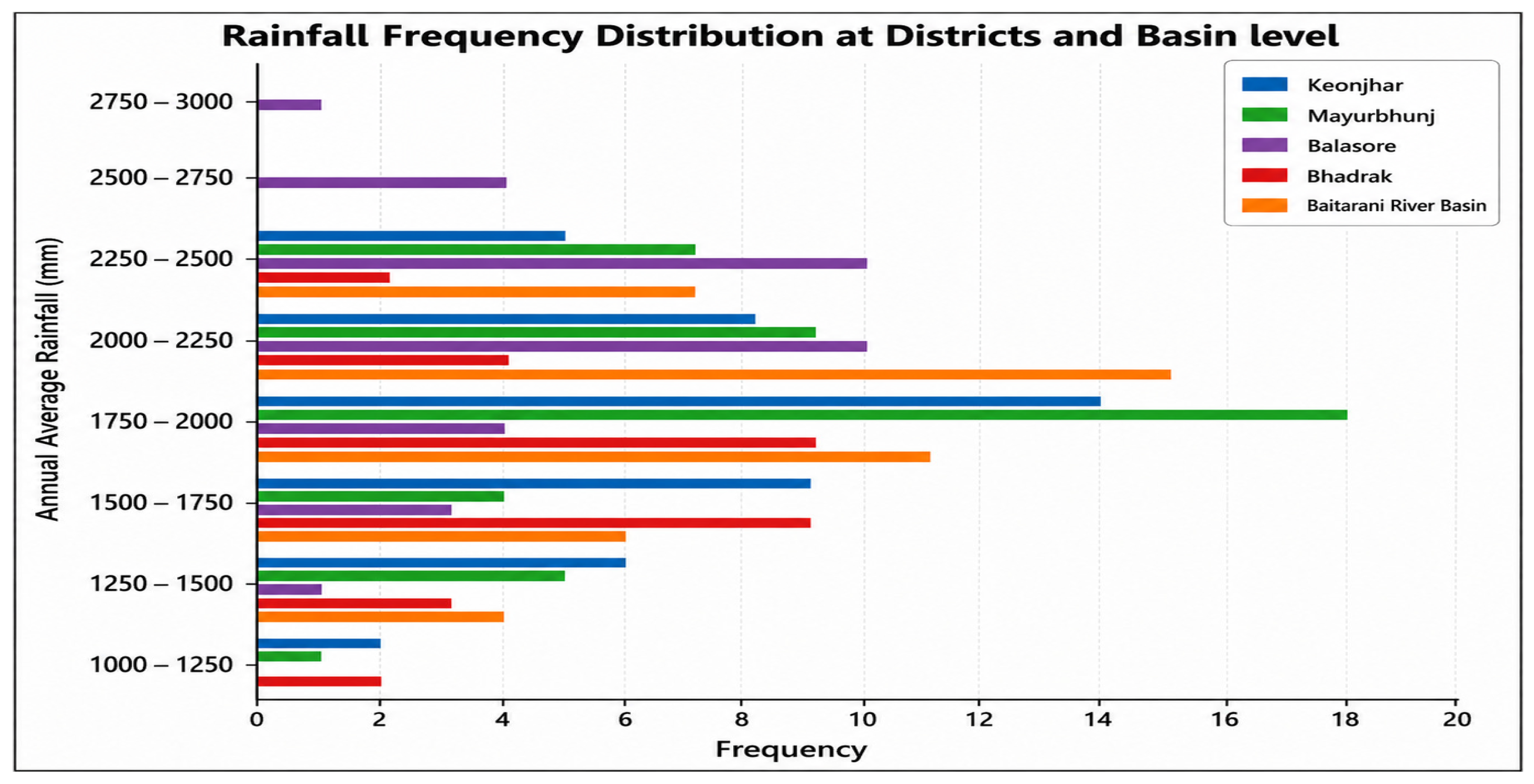
In this section, precipitation data from four districts within the Baitarani River Basin were analyzed to investigate temporal and spatial rainfall variability. The analysis was conducted using the quality-controlled rainfall dataset after treatment of missing values. The variation in annual rainfall across the four districts is presented in Figure 3. Balasore records the highest average annual rainfall (approximately 2085 mm) and shows a comparatively wider interquartile range, indicating greater rainfall variability among the districts. In contrast, Bhadrak exhibits the lowest average rainfall (approximately 1675 mm), with relatively lower variability. A few outliers are also observed, representing occasional extreme rainfall years. Figure 4 indicates that most annual rainfall values are concentrated between 1500 mm and 2000 mm, with the highest frequency occurring around 1700–1800 mm.

The coefficient of variation (CV) values reported in Table 1 provide the statistical basis for distributional comparisons across districts. Balasore shows the highest annual rainfall variability (CV = 0.15) and the widest interquartile range, consistent with greater exposure to cyclonic rainfall events. All interpretive statements regarding distributional properties are grounded in the CV, kurtosis, and skewness values reported in Table 1, rather than subjective visual assessment alone.

3.1. Homogeneity Test (Shift Point Detection)

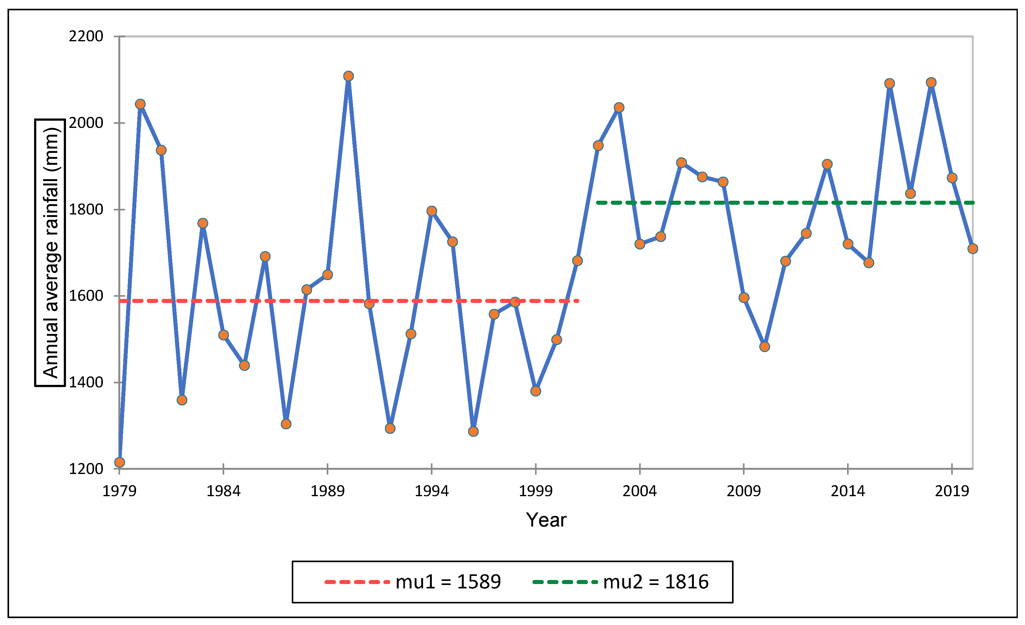
The Pettitt, SNHT, and Buishand tests were applied to identify possible change points in the rainfall series (

Table 2. Results of homogeneity test on rainfall (mm) series on different districts.

Districts	Pettitt Test			SNHT Test			Buishand Test
	K	t	P	T0	t	P	Q	t	P
Keonjhar	249	2001	0.011	9.66	2001	0.014	10.15	2001	0.008
Mayurbhunj	243	2001	0.014	8.215	2001	0.039	9.357	2001	0.015
Bhadrak	175	2001	0.226	4.996	1979	0.278	5.626	2001	0.328
Balasore	163	2001	0.334	4.962	1979	0.295	5.446	2001	0.378
Baitarani	207	2001	0.069	5.842	2001	0.158	7.891	2001	0.062

and Figure 5). The results indicate statistically significant shifts around 2001 for Keonjhar and Mayurbhunj districts. For Keonjhar, Pettitt test yielded K = 249 with p = 0.011, while SNHT (p = 0.014) and Buishand (p = 0.008) also indicated significant change points. Similarly, Mayurbhunj exhibited significant shifts with K = 243 and p = 0.014, supported by SNHT (p = 0.039) and Buishand (p = 0.015). In contrast, Bhadrak (p = 0.226) and Balasore (p = 0.334) showed no statistically significant shifts, although all three tests identified 2001 as a potential transition year. At the basin scale, the results (K = 207, p = 0.069) suggest a moderate but statistically non-significant shift around 2001. The results suggest that 2001 may represent a transition period in rainfall behavior for certain parts of the basin, particularly in Keonjhar and Mayurbhunj districts, where statistically significant shifts were observed.

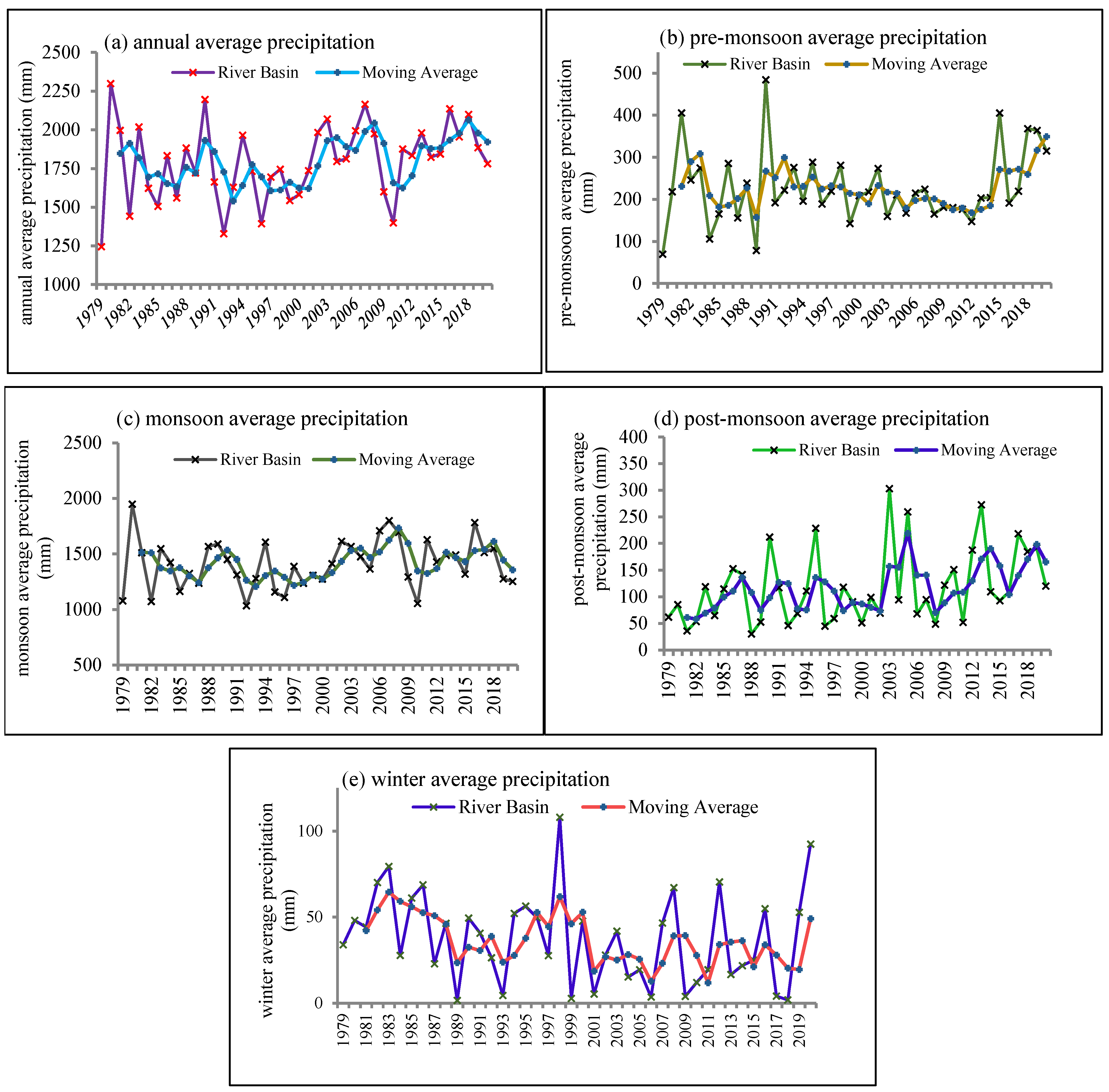
Based on the change points identified around 2001 from the Pettitt, SNHT, and Buishand homogeneity tests, the 42-year rainfall dataset was divided into two periods: Period I (1979–2001) and Period II (2002–2020) for comparative trend analysis. Splitting the data helps us see trends that might be hidden when looking at the entire period together. The 3-year moving average (Figure 6) also shows that, after 2001, monsoon rainfall started declining after a period of being fairly steady.

3.2. District-Wise Trends in Annual and Seasonal Rainfall

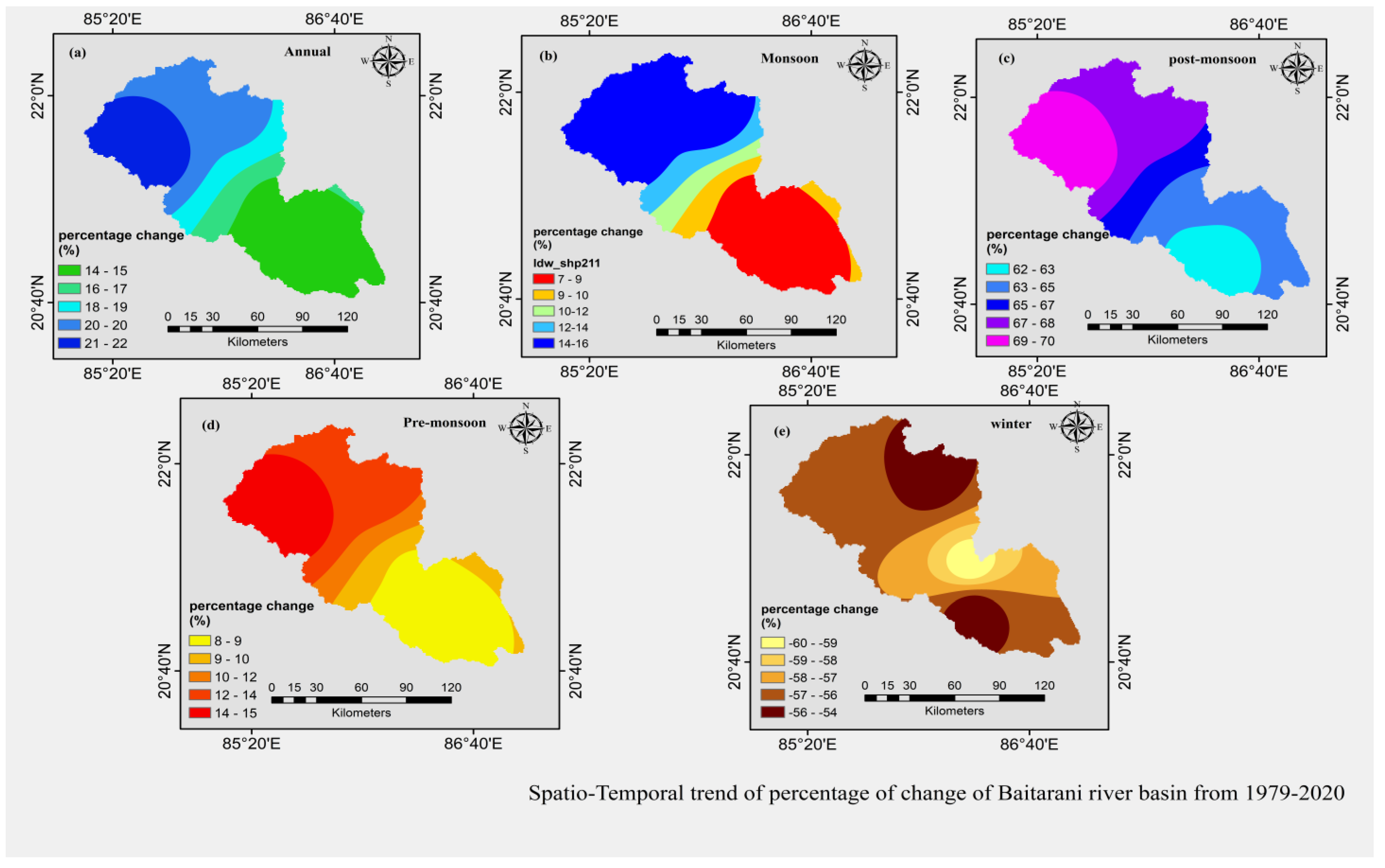
We used the Mann–Kendall test and Sen’s Slope estimator to check rainfall trends over three time periods.

Table 3. Average annual and seasonal rainfall time series.

1979–2020

Annual

Pre-Monsoon

Monsoon

Post-Monsoon

Winter

Districts

Test Z

SL

β

% Change

Test Z

SL

β

% Change

Test Z

SL

β

% Change

Test Z

SL

β

% Change

Test Z

SL

β

% Change

Keonjhar

2.4

*

0.7

21.8

0.8

#

0.3

14.9

1.8

+

1.2

15.9

2.4

*

0.7

69.7

−1.4

#

−0.2

−57.9

Mayurbhunj

2.4

*

0.7

19.2

0.7

#

0.3

13.2

1.7

+

1.3

16.3

2.5

*

0.7

67.5

−1.5

#

−0.5

−55.9

Balasore

1.3

#

0.6

13.8

0.3

#

0.1

7.6

0.8

#

0.8

7.5

2.3

*

0.5

62.3

−1.3

#

−0.3

−55.9

Bhadrak

1.8

+

0.5

14.7

0.2

#

0.2

8.6

0.9

#

0.6

8.1

2.4

*

0.6

63.6

−1.6

#

−0.3

−61.0

1979–2001 (Before Shift Point)

Keonjhar

−0.5

#

−0.4

−6.1

0.4

#

0.3

9.6

−0.7

#

−1.1

−7.9

0.5

#

0.3

16.9

−0.6

#

−0.4

−40.7

Mayurbhunj

−0.2

#

−0.3

−5.0

0.7

#

0.6

17.6

−0.5

#

−1.0

−7.4

0.9

#

0.3

23.4

−0.8

#

−0.5

−28.7

Balasore

−0.9

#

−0.8

−11.4

−0.1

#

−0.1

−2.0

−1.0

#

−2.4

−13.7

0.1

#

0.1

5.8

−1.1

#

−0.7

−70.9

Bhadrak

−0.6

#

−0.3

−5.9

−0.1

#

−0.2

−5.2

−0.3

#

−0.3

−2.5

0.2

#

0.1

4.0

−1.6

#

−0.6

−63.0

2002–2020 (After Shift Point)

Keonjhar

−0.3

#

−0.2

−1.9

2.1

*

1.9

43.8

−1.5

#

−3.2

−17.5

1.1

#

1.1

41.0

0.4

#

0.3

31.8

Mayurbhunj

−0.3

#

−0.2

−2.4

1.9

+

1.5

36.3

−1.3

#

−2.8

−14.7

0.9

#

1.0

36.4

0.3

#

0.5

31.8

Balasore

−0.3

#

−0.2

−1.8

1.7

+

1.4

38.6

−1.3

#

−3.3

−14.3

1.0

#

0.9

37.0

0.8

#

0.6

54.2

Bhadrak

0.5

#

0.1

1.2

1.4

#

1.4

36.7

−1.1

#

−1.7

−9.5

1.3

#

1.0

39.7

0.8

#

0.5

57.9

Where SL is significance level, ***, **, and * values show significance level at 1% (2.577), 5% (1.96), and 10% (1.645), respectively; # indicates non-significant trend; negative (−) and positive (+) values indicate the decreasing and increasing trends, respectively.

shows the results and Figure 7 shows how these trends vary across the districts.

3.2.1. Entire Time Series (1979–2020)

The trend analysis for the period 1979–2020 indicates statistically significant increasing annual rainfall trends in Keonjhar (Z = 2.4, β = 0.7 mm/year) and Mayurbhunj (Z = 2.4, β = 0.7 mm/year). In contrast, Balasore (Z = 1.3, β = 0.6 mm/year) and Bhadrak (Z = 1.8, β = 0.5 mm/year) exhibited increasing tendencies that were not statistically significant. Seasonally, post-monsoon rainfall showed statistically significant increasing trends across all districts, with Z values ranging from 2.3 to 2.5 and β values between 0.5 and 0.7 mm/year. Winter rainfall exhibited decreasing tendencies, although these trends were statistically non-significant. Similarly, monsoon rainfall showed no statistically significant trend during the study period. However, this overall picture hides important differences between the earlier and later year as shown below.

3.2.2. Before Shift Point (1979–2001)

The first sub-period (1979–2001) presents a generally flat to slightly negative annual trend in three districts, with Balasore showing a decline of approximately –0.8 mm per year (not significant at the 95% level) and Keonjhar and Bhadrak both near zero. Mayurbhunj district is the only exception, with a weak but positive annual slope of +0.4 mm per year. Seasonally, the early-period monsoon trends were largely flat, and the pre-monsoon season actually shows a marginal decline in rainfall across all four districts (averaging –0.5 mm per year), possibly reflecting a period of relative climatic stability or early water-management practices that did not favor intense summer rains.

3.2.3. After Shift Point (2002–2020)

After the 2001 change point, variations in seasonal rainfall patterns were observed across the districts of the Baitarani River Basin. Although most yearly trends were statistically non-significant, monsoon rainfall exhibited declining tendencies in all districts, ranging from 1.7 to 3.3 mm/year. The largest decreases were observed in Balasore (−3.3 mm/year; −14.3%), followed by Keonjhar (−3.2 mm/year; −17.5%) and Mayurbhunj (−2.8 mm/year; −14.7%). In contrast, pre-monsoon rainfall showed increasing tendencies, with a statistically significant rise in Keonjhar (1.9 mm/year; +43.8%), while other districts also displayed positive but non-significant trends. Post-monsoon and winter rainfall similarly indicated increasing tendencies during this period, although these changes were not statistically significant.

The combined analysis of MK Test Z, Sen’s slope (β), and homogeneity parameters (K, t, p) identified a significant change point in 2001 across the rainfall series in the Baitarani River Basin. The results indicate contrasting seasonal rainfall trends before and after the detected shift point. Post-2001 analysis shows declining monsoon rainfall trends in several districts, with Sen’s slope values reaching up to −3.3 mm/year, while pre-monsoon and post-monsoon rainfall exhibited increasing trends, with β values up to +1.9 mm/year and +0.7 mm/year, respectively. In addition, winter rainfall displayed declining tendencies during the long-term analysis period. Spatial variability was also observed among districts, particularly in Bhadrak and Balasore, indicating heterogeneous rainfall behavior across the basin. Overall, the findings suggest increasing seasonal variability and temporal redistribution of rainfall despite slight increases in annual rainfall totals

The reliability of the interpolated surfaces largely depends on the number, density, and spatial distribution of the meteorological stations used in the analysis. In areas with sparse observational coverage, the generated isolines and isozones may appear generalized or artificially smooth, and may not fully capture local spatial variability. Therefore, the interpolation maps should be interpreted as indicative representations of regional trends rather than exact depictions of conditions between observation points. The limitations associated with the interpolation technique and station distribution should be considered while interpreting the spatial patterns shown in Figure 7.

3.3. Entropy-Based Rainfall Analysis Using Marginal Disorder Index (MDI)

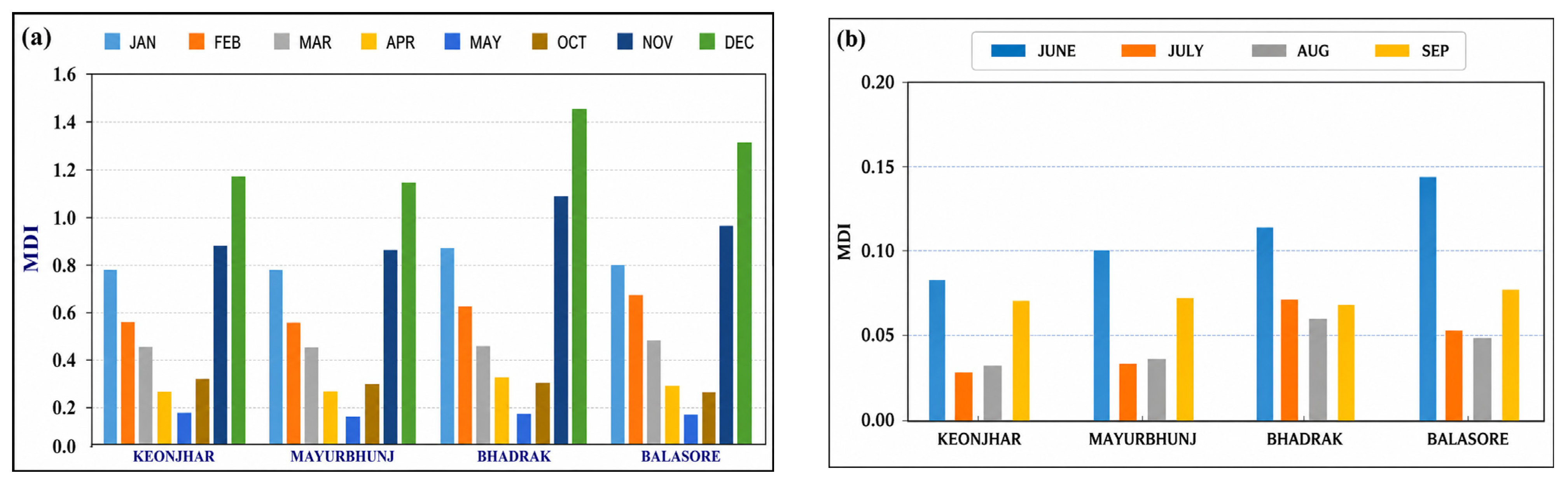
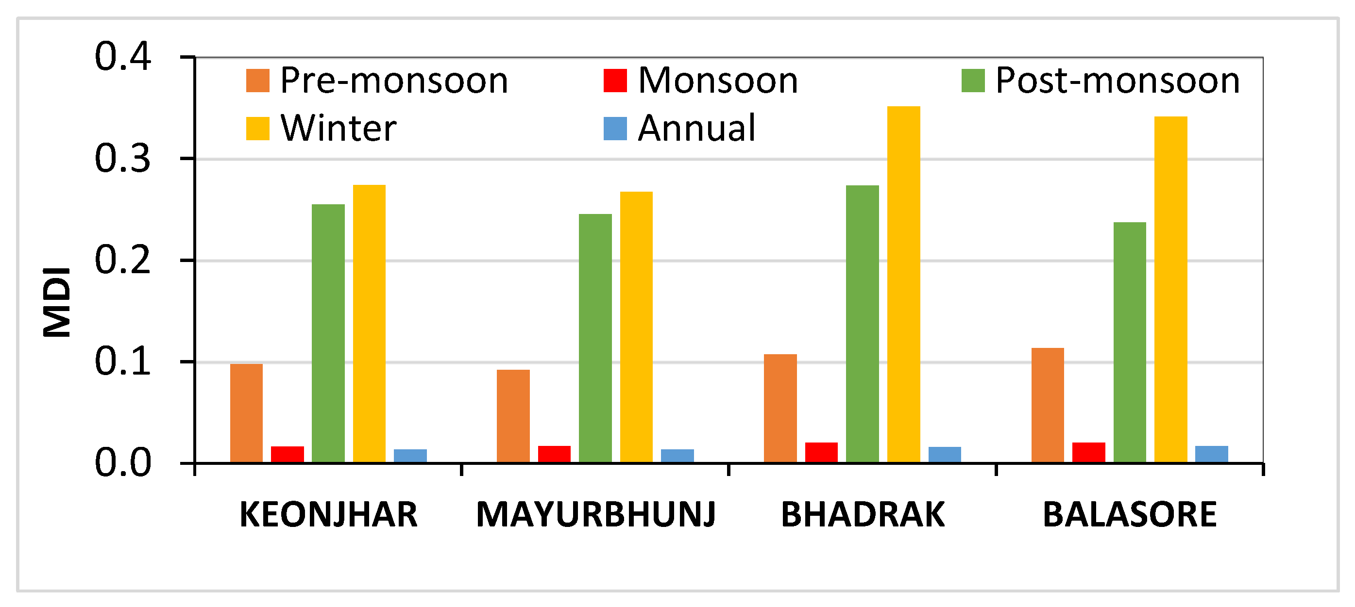
MDI test was carried out for the four districts across Baitarani Basin using monthly, seasonal and annual rainfall data for 42 years from 1979 to 2020. MDI was used to assess the temporal variability and distribution of rainfall across different time scales [

Table 4. MDI for monthly rainfall series (1979–2020).

Districts	Jan	Feb	Mar	Apr	May	Jun	Jul	Aug	Sep	Oct	Nov	Dec
Keonjhar	0.77	0.55	0.45	0.23	0.16	0.09	0.04	0.04	0.07	0.29	0.89	1.17
Mayurbhunj	0.78	0.55	0.45	0.23	0.15	0.10	0.04	0.04	0.07	0.27	0.88	1.15
Bhadrak	0.88	0.59	0.47	0.31	0.14	0.12	0.07	0.06	0.07	0.30	1.11	1.44
Balasore	0.81	0.66	0.47	0.29	0.15	0.15	0.05	0.05	0.08	0.25	0.97	1.35
Baitarani Basin	0.79	0.57	0.45	0.25	0.14	0.10	0.04	0.04	0.07	0.27	0.92	1.24

and

Table 5. MDI for seasonal rainfall series (1979–2020).

Districts	Pre-Monsoon	Monsoon	Post-Monsoon	Winter	Annual
Keonjhar	0.10	0.02	0.25	0.27	0.01
Mayurbhunj	0.09	0.02	0.25	0.27	0.01
Bhadrak	0.11	0.02	0.27	0.35	0.02
Balasore	0.11	0.02	0.24	0.34	0.02
Baitarani Basin	0.10	0.02	0.24	0.30	0.01

; Figure 8a,b and Figure 9]. Lower MDI values generally indicate a relatively uniform distribution of rainfall over time, whereas higher MDI values reflect greater irregularity and concentration in rainfall occurrence. Thus, increasing MDI values suggest higher temporal variability in rainfall patterns, which may influence hydrological processes and water resource management in the Baitarani River Basin.

Looking at individual months, MDI values are the lowest during the monsoon months (0.03 to 0.07 across all districts), showing that rainfall from June to September is steady and predictable. In contrast, December shows the highest disorder, especially in Bhadrak (1.44) and Balasore (1.35), reflecting how unpredictable post-monsoon rainfall can be.

Looking at seasons, monsoon rainfall has the lowest MDI values (0.016–0.020), confirming it is the most reliable water source. Winter (0.27–0.35) and post-monsoon (0.23–0.27) seasons show much higher unpredictability. Bhadrak and Balasore consistently showed the highest MDI values across all seasons, meaning coastal districts face greater uncertainty in rainfall than inland areas.

Although the annual MDI values remain low across all districts (0.013–0.017), indicating relatively stable and predictable annual rainfall totals, this annual-scale assessment masks significant seasonal variations in rainfall distribution. The observed seasonal shifts suggest changes in the timing and concentration of rainfall, which directly influence water availability, agricultural planning, and irrigation demand within the Baitarani River Basin. Therefore, despite the apparent annual stability, understanding seasonal rainfall variability is essential for achieving the main objective of the study, namely effective basin-scale water resource management and climate-resilient planning.

4. Discussions

This study provides a comprehensive assessment of rainfall trends and variability in the Baitarani River Basin over the period 1979–2020. The Baitarani River in Odisha is a crucial source of water for about seven million people across various districts and urban centers. There are multiple problems and challenges faced in the basin. Baitarani Basin is dominated by the indigenous tribal population bearing high pressure of deforestation, water scarcity, low agricultural productivity, and climate variability. At the same time, the delta region witnesses flooding particularly during monsoon. There are issues related to access, availability and quality of surface and groundwater, irrigation management, delta salinity and mangrove erosion. To address and plan these challenges, an understanding of the spatio-temporal response of the rainfall is of paramount need. This will help the basin planner for managing the water resource, especially during the climate-induced variability in the river basins. Accordingly, this study investigates the rainfall trends and variability in the Baitarani River Basin using high-resolution gridded rainfall data. The study employed MK test, SSE, multiple change point detection tests and entropy-based marginal disorder index to assess the existing trends, shift point, and rainfall variability.

The 42-year rainfall statistical analysis across the four districts indicated visible regional climatic influences, possibly due to the coastal proximity of these districts. Balasore district exhibited higher and more erratic rainfall compared to other districts. Further, the frequency distribution analysis of rainfall across the four districts showed a peak frequency around 1700–1800 mm. This also conforms to the increasing rainfall variability with deficient and excess rainfall events becoming more frequent in the region.

In this study, shift analysis was performed using Pettitt test, Buishand test and SNHT test. All the tests identified 2001 as a significant change point in basin rainfall behavior. Shift point detection is an important step while analyzing a climatic time series to understand the impact in the recent past (after the shift point). The shift point also became a transition point in the regional hydro-climatic regime. Further investigation into the causes of the observed shift year (2001) in the Baitarani Basin led us to the rapid land use changes because of urban growth. It has also been seen that forest cover, agricultural lands and water bodies are transforming to mining areas, built-up areas and industrial settlements.

In the study, rainfall trends were investigated using non-parametric MK test and SSE. The analysis revealed that, although total annual rainfall shows increasing trends in some districts, the decline in monsoon rainfall post 2001 is worrying in nature. A declining monsoon will result in overall decline in its contribution to the total runoff and groundwater recharge in the basin. This impact has many ramifications in the basin’s water availability. In other words, the agricultural production and water needs of the basin will be considerably compromised in the long run. Equally important are the findings of the pre-monsoon and post-monsoon rainfall trends in the basin. It was found that the pre-monsoon rainfall (β = +1.9 mm/year) and post-monsoon rainfall (β = +0.7 mm/year) suggest a temporal redistribution of rainfall, leading to short-duration, high-intensity flow events rather than sustained flows. This shift can increase the risk of flash floods during early and late seasons, while simultaneously reducing water availability during peak agricultural demand periods. The winter rainfall is declining in the basin.

Overall, the results indicate that, despite a slight increase in annual rainfall, the basin is shifting toward a more irregular and less reliable flow regime, characterized by declining monsoon-driven flows, increased seasonal variability, and higher hydrological uncertainty. The results also indicated that, while annual rainfall shows an increasing trend in some districts, this increase is not uniform across seasons. Instead, a significant redistribution of rainfall is observed. The seasonal variability in rainfall is most challenging to plan for agriculture. A reduced monsoon rainfall will impact the overall water availability, whereas a diminishing post-monsoon rainfall will impact the early sowing and adoption of rabi crops. Winter rainfall variability, although not significant, will highly impact the rabi crops. The identification of 2001 as the shift point marks a transition in rainfall behavior. Before 2001, rainfall patterns were relatively stable, particularly during the monsoon season. However, after 2001, a consistent decline in monsoon rainfall is observed across all districts, accompanied by increasing trends in pre-monsoon and post-monsoon rainfall. This shift suggests a movement away from monsoon-dominated rainfall towards a more irregular seasonal distribution.

The analysis further revealed visible differences of rainfall variability between coastal and inland districts (Figure 7). Districts like Balasore and Keonjhar show more variable rainfall and larger drops in monsoon rainfall after 2001 compared to districts like Bhadrak and Mayurbhunj. Looking at the whole, there is a west-to-east pattern; inland districts in the west witnessed a larger increase in rainfall, while the coastal district in the east witnessed a marginal increase. After 2001, this pattern reversed—coastal districts experienced greater declines in monsoon rainfall than inland areas. This suggests that coastal areas are more vulnerable to changing rainfall pattern. These differences are likely due to the factors like hills, distance from the sea, and recurring cyclones. In addition, the entropy-based variability analysis highlights increasing uncertainty in rainfall patterns, especially in Bhadrak and Balasore districts. This increased variability indicates a higher risk of extreme events such as floods and droughts, which can significantly impact agriculture, water supply, and basin management. A limitation of this study relates to the use of the IDW method for generating spatial maps, particularly in sparsely monitored areas where the method may produce smoother and sometimes artificial spatial patterns. However, station distribution should be considered while interpreting the spatial patterns. The interpolated results depend on the number and distribution of meteorological stations, and uneven station coverage may reduce the accuracy of local precipitation patterns. Therefore, the maps should be considered as generalized representations of regional climatic trends rather than exact spatial distributions.

5. Conclusions

This study shows that changes in rainfall occur across seasons matter just as much as changes in the total amount of rainfall. Because of this, water planning and management in the Baitarani Basin needs to consider both shifting rainfall patterns and growing variability. Practical steps such as better rainfall forecasting, smart reservoir use, expanding water storage, and promoting climate-resilient farming will be important in dealing with future challenges. Overall, the study suggests that rainfall behavior in the Baitarani River Basin is changing noticeably, and managing water resources will require flexible and well-coordinated approaches as the climate continues to change. The variability witnessed in the basin can be attributed to multiple local topographic and land use factors, but larger factors like global warming, rapid urbanization and industrialization, deforestation, change in cyclone behavior, or natural climate patterns such as ENSO cannot be denied. However, further research is needed to understand the exact causes. The rainfall variability in the basin cannot be controlled but certainly the impact due to this can be mitigated through appropriate management strategies. These include adopting integrated basin planning, increased scope for groundwater recharge, promoting the use of seasonal climate forecasts for operational decision-making, and strengthening the resilience of riparian and estuarine ecosystems sensitive to altered freshwater inflows. Overall, these findings show that water management plans must be revisited, seasonal forecasts improved, and flexible strategies adopted to deal with a new rainfall reality in the Baitarani Basin.

References

1. Mehta, D.; Yadav, S.M. An analysis of rainfall variability and drought over Barmer District of Rajasthan, Northwest India. Water Supply 2021, 21, 2505–2517. [Google Scholar] [CrossRef] [Scilit]
2. Koutsoyiannis, D. Revisiting the global hydrological cycle: Is it intensifying? Hydrol. Earth Syst. Sci. 2020, 24, 3899–3932. [Google Scholar] [CrossRef] [Scilit]
3. Krishn, P.; Kumar, G.; Kale, G.D. Trend analyses in gridded rainfall data over the Sabarmati basin. Mausam 2022, 73, 295–306. [Google Scholar] [CrossRef] [Scilit]
4. Kumar, D. Climate change, a strong threat to food security in india: With special reference to Gujarat. In Climate Change Impacts on Natural Resources, Ecosystems and Agricultural Systems; Springer: Cham, Switzerland, 2023; pp. 153–173. [Google Scholar]
5. Taxak, A.K.; Murumkar, A.R.; Arya, D.S. Long term spatial and temporal rainfall trends and homogeneity analysis in Wainganga basin, Central India. Weather Clim. Extrem. 2014, 4, 50–61. [Google Scholar] [CrossRef] [Scilit]
6. Modarres, R.; da Silva, V.d.P.R. Rainfall trends in arid and semi-arid regions of Iran. J. Arid Environ. 2007, 70, 344–355. [Google Scholar] [CrossRef] [Scilit]
7. Patakamuri, S.K.; Muthiah, K.; Sridhar, V. Long-Term homogeneity, trend, and change-point analysis of rainfall in the arid district of Ananthapuramu, Andhra Pradesh State, India. Water 2020, 12, 211. [Google Scholar] [CrossRef] [Scilit]
8. Mitra, A.K.; Momin, I.M.; Rajagopal, E.N.; Basu, S.; Rajeevan, M.N.; Krishnamurti, T.N. Gridded daily Indian monsoon rainfall for 14 seasons: Merged TRMM and IMD gauge analyzed values. J. Earth Syst. Sci. 2013, 122, 1173–1182. [Google Scholar] [CrossRef] [Scilit]
9. Ahmad, I.; Tang, D.; Wang, T.; Wang, M.; Wagan, B. Precipitation trends over time using Mann-Kendall and spearman’s Rho tests in swat river basin, Pakistan. Adv. Meteorol. 2015, 2015, 431860. [Google Scholar] [CrossRef] [Scilit]
10. Chandniha, S.K.; Kansal, M.L. Prioritization of sub-watersheds based on morphometric analysis using geospatial technique in Piperiya watershed, India. Appl. Water Sci. 2017, 7, 329–338. [Google Scholar] [CrossRef] [Scilit]
11. Mooley, D.A.; Parthasarathy, B. Indian summer monsoon and El Nino. Pure Appl. Geophys. 1983, 121, 339–352. [Google Scholar] [CrossRef] [Scilit]
12. Ramola, M.; Mishra, P.K.; Nayak, P.C.; Thakur, A. Long-term rainfall trend analysis for six homogeneous monsoon regions of India. Curr. Sci. 2025, 128, 915. [Google Scholar] [CrossRef] [Scilit]
13. Singh, L.; Khare, D.; Mishra, P.K.; Pingale, S.; Thakur, H. Spatial and temporal precipitation trends of proposed smart cities based on homogeneous monsoon regions across India. J. Water Land Dev. 2020, 47, 150–159. [Google Scholar] [CrossRef] [Scilit]
14. Kundu, S.; Khare, D.; Mondal, A.; Mishra, P.K. Analysis of spatial and temporal variation in rainfall trend of Madhya Pradesh, India (1901–2011). Environ. Earth Sci. 2015, 73, 8197–8216. [Google Scholar] [CrossRef] [Scilit]
15. Kumar, V.; Jain, S.K.; Singh, Y. Analysis of long-term rainfall trends in India. Hydrol. Sci. J. 2010, 55, 484–496. [Google Scholar] [CrossRef] [Scilit]
16. Guhathakurta, P.; Rajeevan, M. Trends in the rainfall pattern over India. Int. J. Climatol. 2008, 28, 1453–1469. [Google Scholar] [CrossRef] [Scilit]
17. Krishnakumar, K.N.; Rao, G.P.; Gopakumar, C.S. Rainfall trends in twentieth century over Kerala, India. Atmos. Environ. 2009, 43, 1940–1944. [Google Scholar] [CrossRef] [Scilit]
18. Rajeevan, M.; Pai, D.S.; Anil Kumar, R.; Lal, B. New statistical models for long-range forecasting of southwest monsoon rainfall over India. Clim. Dyn. 2007, 28, 813–828. [Google Scholar] [CrossRef] [Scilit]
19. Sankhua, R.N.; Samal, K.P. Hypsometric Analysis of Brahmani–Baitarani Basin Using ArcGIS. In International Conference on Hydraulics, Water Resources and Coastal Engineering; Springer Nature: Singapore, 2021; pp. 73–83. [Google Scholar]
20. Thakur, A.; Mishra, P.K.; Nema, A.K.; Sahoo, S.P. Spatiotemporal Pattern Assessment of Precipitation for the Wainganga Sub-basin. Curr. World Environ. 2020, 15, 515–525. [Google Scholar] [CrossRef] [Scilit]
21. Thakur, A.; Mishra, P.K.; Nema, A.K.; Sahoo, S.P. Spatio-temporal trends and shift analysis of temperature for Wainganga sub-basin, India. Int. J. Environ. Stud. 2019, 77, 464–479. [Google Scholar] [CrossRef] [Scilit]
22. Jha, R.; Singh, V.P.; Singh, V.; Roy, L.B.; Thendiyath, R. (Eds.) Climate Change Impacts on Water Resources; Water Science and Technology Library; Springer: Cham, Switzerland, 2021; Volume 98, pp. 293–306. [Google Scholar]
23. Pandi, D.; Kothandaraman, S.; Kumarasamy, M.; Kuppusamy, M. Assessment of land use and land cover dynamics using geospatial techniques. Pol. J. Environ. Stud. 2022, 31, 2779–2786. [Google Scholar] [CrossRef] [Scilit]
24. Mohseni, U.; Agnihotri, P.G.; Pande, C.B.; Durin, B. Understanding the climate change and land use impact on streamflow in the present and future under CMIP6 climate scenarios for the Parvara Mula Basin, India. Water 2023, 15, 1753. [Google Scholar] [CrossRef] [Scilit]
25. Patra, T.R.; Pathy, A.C. Long-Term Temperature Trends in the Upper Baitarani Basin, Odisha Analyzing Regional Climate Variability. J. Geogr. Environ. Earth Sci. Int. 2024, 28, 44–56. [Google Scholar] [CrossRef] [Scilit]
26. Dahm, R.J.; Singh, U.K.; Lal, M.; Marchand, M.; Sperna Weiland, F.C.; Singh, S.K.; Singh, M.P. Downscaling GCM data for climate change impact assessments on rainfall: A practical application for the Brahmani-Baitarani River basin. Hydrol. Earth Syst. Sci. Discuss. 2016, 2016, 1–42. [Google Scholar] [CrossRef] [Scilit]
27. Swain, S.S.; Mishra, A.; Sahoo, B.; Chatterjee, C. Comparative Impact Assessment of Climate Change and Land-Use Alteration on Decadal Water Balance Components: A Case Study on The Baitarani River Basin, Odisha. ESS Open Arch. 2022. preprint. [Google Scholar] [CrossRef] [Scilit]
28. Shukla, R.; Khare, D.; Tiwari, P.; Mishra, P.K.; Gupta, S. Analysis of Long Term Temperature Trend for Madhya Pradesh, India (1901–2005). Curr. World Environ. 2017, 12, 68–79. [Google Scholar] [CrossRef] [Scilit]
29. Shah, S.; Khare, D.; Mishra, P.K.; Singh, L. Historical Trend Analysis of a Terai Himalayan district of Nepal: A Case Study. Int. Eng. Technol. 2017, 3, 542–560. [Google Scholar]
30. Samal, K.P.; Dhara, P.; Tarai, A. Groundwater Pollution: An Overview of Geogenic and Anthropogenic Sources. In International Conference on Recent Developments in Sustainable Infrastructure; Springer Nature: Singapore, 2023; pp. 285–298. [Google Scholar]
31. Tarai, A.K.; Samal, K.P.; Bera, D.K. Temporal Trends in Groundwater Quality Parameters of Bhubaneswar City, Odisha: A Statistical Analysis Using Mann–Kendall and Sen’s Slope Estimator. In International Conference on Recent Developments in Sustainable Infrastructure; Springer Nature: Singapore, 2023; pp. 247–258. [Google Scholar]
32. Mishra, P.K.; Singh, H.; Das, S.; Chandniha, S.K. Entropy-based measurement of long-term precipitation variability across India. In Advances in Hydrology and Climate Change; Apple Academic Press: Palm Bay, FL, USA, 2022; pp. 375–392. [Google Scholar]
33. Sinam, R. Rainfall trend analysis of Baitarani River Sub-basin Odisha. Int. J. Adv. Res. 2019, 7, 569–575. [Google Scholar] [CrossRef] [Scilit] [PubMed]
34. Gupta, S.; Gupta, U. Analysis of Trends in Temperature and Precipitation and its Impact on Hydrology of a Coastal River Basin in Eastern India. J. Indian Soc. Coast. Agric. Res. 2020, 38, 85–94. [Google Scholar]
35. Sahoo, S.; Samal, K.P.; Mishra, P.K. Historical Trend Analysis: A Case Study of Baitarani River Basin. In International Conference on Recent Developments in Sustainable Infrastructure; Springer Nature: Singapore, 2023; pp. 217–226. [Google Scholar]
36. Henry, M. Nonparametric tests against trend. Econometrica 1945, 13, 245–259. [Google Scholar] [CrossRef] [Scilit]
37. Shannon, C.E. A mathematical theory of communication. Bell Syst. Tech. J. 1948, 27, 379–423. [Google Scholar] [CrossRef] [Scilit]
38. Chow, S.C.; Tse, S.K. Outlier detection in bioavailability/bioequivalence studies. Stat. Med. 1990, 9, 549–558. [Google Scholar] [CrossRef] [Scilit]
39. Hamed, K.H.; Ramachandra Rao, A. A modified Mann-Kendall trend test for autocorrelated data. J. Hydrol. 1998, 204, 182–196. [Google Scholar] [CrossRef] [Scilit]
40. Karpouzos, D.K.; Kavalieratou, S.; Babajimopoulos, C. Trend analysis of precipitation data in Pieria Region (Greece). Eur. Water 2010, 30, 30–40. [Google Scholar]
41. Bayazit, M.; Önöz, B. To prewhiten or not to prewhiten in trend analysis? Hydrol. Sci. J. 2007, 52, 611–624. [Google Scholar] [CrossRef] [Scilit]
42. Sen, P.K. Estimates of the regression coefficient based on Kendall’s Tau. J. Am. Stat. Assoc. 1968, 63, 1379–1389. [Google Scholar] [CrossRef]
43. Pettitt, A.N. A non-parametric to the approach problem. Appl. Stat. 1979, 28, 126–135. [Google Scholar] [CrossRef] [Scilit]
44. Alexandersson, H. A homogeneity test applied to precipitation data. J. Climatol. 1986, 6, 661–675. [Google Scholar] [CrossRef] [Scilit]
45. Buishand, T.A. Some methods for testing the homogeneity of rainfall records. J. Hydrol. 1982, 58, 11–27. [Google Scholar] [CrossRef] [Scilit]
46. Gemmer, M.; Becker, S.; Jiang, T. Observed monthly precipitation trends in China 1951–2002. Theor. Appl. Climatol. 2004, 77, 39–45. [Google Scholar] [CrossRef] [Scilit]
Figure 1. Location map. (a) Country of India showing the national context of the study area, (b) Odisha state map presenting the study area, and (c) the Baitarani River Basin map provides detailed river stream along with elevation of the area under investigation.
Earth 07 00098 g001
Figure 2. Flowchart showing overall methodology adopted in the present study.
Earth 07 00098 g002
Figure 3. Box plots showing annual average rainfall of different districts in and around Baitarani River Basin.
Earth 07 00098 g003
Figure 4. Frequency distribution of annual average rainfall (X-axis) of different districts in and around Baitarani River Basin.
Earth 07 00098 g004
Figure 5. Shift point detected for the annual average rainfall over Baitarani River Basin. “mu” defined as the “period average value” or “mean value of the corresponding period”.
Earth 07 00098 g005
Figure 6. Spatial distribution of average precipitation during 1979–2020 in the Baitarani River Basin: (a) annual average precipitation, (b) pre-monsoon average precipitation, (c) monsoon average precipitation, (d) post-monsoon average precipitation, and (e) winter average precipitation.
Earth 07 00098 g006
Figure 7. Rainfall trends and percentage of change during 1979–2020 over four districts in and around Baitarani River Basin of (a): annual, (b): monsoon, (c): post-monsoon, (d): pre-monsoon and (e): winter.
Earth 07 00098 g007
Figure 8. MDI of bar graph on (a) non-monsoon and (b) monsoon months.
Earth 07 00098 g008
Figure 9. Bar graph of MDI for seasonal rainfall series.
Earth 07 00098 g009