


Abstract
Accurate quantification of surface runoff is required for the appropriate design of storage structures, irrigation patterns, waterways, erosion control structures, water harvesting projects, and groundwater development schemes. However, the paucity of runoff data in Iraq and Iran is a serious obstacle. The soil conservation service–curve number (SCS–CN) method is applied in conjunction with remote sensing (RS) and geographic information system (GIS) to predict the surface runoff in the Shatt Al-Arab Region. In the present study, the Shatt Al-Arab Region is defined as the drainage areas and lateral sub-basins that contribute direct surface runoff to the main channel between Qurna city and the Arabian Gulf. Rainfall, land use/land cover (LULC), hydrologic soil group (HSG), and slope maps are developed in a GIS platform and processed to produce surface runoff for 35 years (1979–2013). The surface runoff ranges between 163 mm (2008) and 300 mm (1982) with an average of 233 mm yr−1. The average annual surface runoff in the study area is 33.657 km3. A scatter plot constructed to visualize the connection between annual rainfall and annual runoff reveals a significant positive relation (coefficient of determination (r2) = 0.67, probability value (p) < 0.05). The runoff potential is low in the southern parts of the study area and gradually rises towards the northern parts. Cross-validation of the modeled annual runoff with the annual runoff data shows reasonably close matches (r2 = 0.73, p < 0.001) demonstrating the procedure’s suitability.
1. Introduction
Decision-makers in arid and semi-arid areas must develop strategies for exploring new water resources or optimizing the use of existing ones. Runoff is a critical variable in determining a region’s water supply and planning sustainable water resources management [1]. Further, runoff represents a significant source of water quality degradation issues [2]. As water flows over a surface, it collects litter, petroleum, fertilizers, chemicals, and other harmful compounds and releases them into water bodies, which has a detrimental effect on the environment and on human health [3]. Additionally, runoff poses an economic hazard; for example, during erosion, runoff removes the rich layer of topsoil upon which farmers depend to cultivate crops [4]. Moreover, sediments generated by soil erosion can accumulate within drainage channels, causing pipes blockage, reduced flow efficiency, and an increased likelihood of flooding [5]. Thus, simple runoff prediction techniques are critical in hydrologic projects such as water balance calculations [6], soil erosion mitigation, and determining the water yield capability of watersheds [7]. Runoff measurements provide valuable information to hydrologists and water resource planners on water allocation and drought management to ensure sustainable water supplies for various purposes [8]. Measuring the amounts and patterns of runoff can help in developing appropriate strategies to allocate water for purposes such as agriculture, industry, domestic use, and preserving ecosystems [9]. Surface runoff also helps in identifying areas that are most exposed to erosion, which in turn causes serious damage to infrastructure, agricultural lands, and water quality [10]. Moreover, surface runoff measurements are used to identify regions most prone to floods to eventually assist in establishing flood control structures and land use planning [11]. Furthermore, surface runoff data contribute to determining the amount of water infiltrating into the soil that contributes to groundwater recharge, which can help in sustainable groundwater resource management [12]. Finally, surface runoff information aids in evaluating the effects of climate change on water resources. Climate parameters such as rainfall, temperature, and evaporation are key parameters that control surface runoff. Evaluation of the response of surface runoff to these parameters assists to predict what future climate change might cause to water resources, which aids water managers in developing strategies to adapt to the effects of climate change [13]. Furthermore, runoff estimation is essential in water-harvesting projects and dams that store surface flows during episodic rainfall events. Runoff assessment is also important for integrated water management that includes a combination of surface storage use and groundwater use. Such management approaches have proven powerful in arid and semi-arid regions [14,15].
Recent techniques in hydrological analyses have employed machine learning and deep learning models to enhance runoff forecasting. For example, Xu [16] found that incorporating long short-term memory networks with transformer architecture can significantly outperforms traditional runoff prediction models. Likewise, Herath [17] detected that combining hydrological knowledge (e.g., catchment structure, flow connectivity, and water balance) with machine learning techniques enables more accurate rainfall–runoff modelling compared to data-based machine learning methods. Predicting runoff in ungauged watersheds, however, is a critical problem in practical hydrology. For example, in Middle Eastern countries such as Iraq and Iran, precise runoff information is scarce owing to the high expense of installing and maintaining hydrologic gauging stations. As a result, credible data on watershed runoff should be created regularly to aid in the development and maintenance of watershed projects [18]. In the absence of runoff data, estimated direct runoff using the SCS–CN method has produced reliable findings [19]. The SCS–CN approach was established by the United States Department of Agriculture to forecast runoff volume for specific rainfall events [20,21,22,23,24,25]. Due to its simplicity and substantial documentation, the SCS–CN approach is employed globally in a broad variety of hydrological applications by a large number of engineers and practitioners [26]. The primary reasons for its remarkable success are that it is a simple but well-established technique, it uses readily available and well-recorded environmental inputs, and it describes a large number of variables influencing runoff development by combining them into one factor called the curve number [27]. This approach is used to quantify the surface runoff amount in unmeasured watersheds. It is a single entity that incorporates the watershed’s physiographic elements such as area, slope, LULC, and soil properties, as well as climatic aspects such as rainfall. It was first created for small watersheds of less than 15 km2 in area and was subsequently improved for large catchments by including the weighting curve approach with LULC and soil properties inputs [28]. A significant benefit of this approach is that GIS technique can be readily incorporated since the approach’s factors are geographical in nature. Numerous researchers have tried to predict surface runoff by combining conventional data with remote sensing data using the SCS–CN method [29]. The approach has been used for a variety of regions, LULC, and climatic conditions [30,31]. Additionally, it was expanded much beyond its initial scope and became a necessary component of continuous simulation models (e.g., [32,33,34,35]). Many researchers asserted that the SCS–CN can be utilized effectively to predict the runoff depth in the absence of adequate hydrological data (e.g., [36,37]).
The computation of runoff generation in the SCS–CN model relies mainly on CN values, which are strongly influenced by significant runoff-related watershed factors such as soil type, LULC, Antecedent Moisture Condition (AMC), slope, and meteorological system [38]. A low CN indicates that the surface has a strong capacity to absorb water under given rainfall conditions, while high CN values indicate increased surface runoff [39]. The CN can be calculated by using widely accessible curves and tables; however, this is a difficult and time-consuming process. On the other hand, RS and GIS are powerful tools for calculating formula coefficients and model factors in runoff computation. By incorporating RS and GIS into hydrologic models, significant cost and time savings are realized while maintaining high dependability and accuracy [40]. Many research studies have been performed worldwide to simulate surface runoff utilizing RS and GIS methodologies [41]. Nayak [42] and Karunanidhi [29] detected a strong correlation between the observed and modeled runoff depth applying the SCS–CN approach.
The Shatt Al-Arab region is a complex system in term of hydrology and politics. This region is subject to escalating population growth and increasing water demand [43], upstream flow projects [44], water quality degradation [45,46,47,48,49], seawater intrusion [50], and climate-induced water resource reduction [51]. Such challenges are exacerbated by the paucity of monitoring data that are essential for water budget quantification. Despite the vital importance of surface runoff estimation, as highlighted earlier, such estimation displays considerable deficiencies. Previous research has highlighted the increasing vulnerability of the region to reduced freshwater inflows and extreme hydrological conditions, including projected freshwater deficits and saltwater intrusion [52,53], drought and declining river discharge [54], and flow reduction influence on salinity and water quality [55,56]. However, limited attention has been given to spatially distributed runoff estimation, particularly through empirical models. Therefore, the current study bridges this gap by implementing an RS–GIS-based SCS–CN model to identify surface runoff in the Shatt Al-Arab region. Accurate runoff estimates for this water-scarce region provide valuable information for managers and policymakers that can be used in water allocation planning, drought management, soil erosion control, flood risk reduction, groundwater recharge potential assessment, and climate change impacts on water resources evaluation. Thus, the main objectives of the current study are to (i) estimate mean rainfall over the Shatt Al-Arab region using the isohyetal method; (ii) calculate surface runoff levels based on rainfall, LULC, soil characteristics, moisture conditions, and slope; (iii) evaluate the applicability of the SCS-CN model for runoff quantification in a semi-arid region with limited hydrological observations; and (iv) provide runoff information that can support water resources planning, policymaking, and management in the region.
2. Study Area
The Shatt Al-Arab River drains the Euphrates and Tigris basins, as well as the Karkhah and Karun sub-basins (Figure 1) [57]. The river is composed by the convergence of the Tigris and Euphrates rivers at the Qurna city. It runs southeast for about 100 km before forming the boundary between Iran and Iraq for the last 90 km of its course. The Karun River originates from Iran’s Zagros Mountains and runs west via valleys and ridges to Ahvaz city, where it joins the Shatt Al-Arab [58]. The Karkheh River originates from the Zagros Mountains, flows south before veering northwest and emptying into the Hawizah Marsh, and ultimately drains into the Shatt Al-Arab through the Swayb River. The overall area draining into the river is about 144,000 km2 including the Karun and Karkheh sub-basins but excluding the Tigris and Euphrates basins (upstream of Qurna) [57]. Iraq and Iran share the study area, which is extended on both the Mesopotamia zone and Zagros structural zone. The first zone (i.e., the Mesopotamia) is subdivided into three sub-zones; the Tigris, the Euphrates, and the Zubair [59]. The Euphrates and Tigris sub–zones are extended outside of the Shatt Al-Arab region, while the Zubair sub-zone is extended inside it. The Zubair sub-zone is dominated by clastic lithological units, with limestone confined to its top portions [60]. The Zubair sub-zone is defined by several elongated folds that have a direction of north–south to northwest–southeast, outlining the main oil fields in the Basra Governorate [61]. These Late Cretaceous anticline folds resemble basement rocks and are impacted by faulting [62]. The second zone (i.e., the Zagros structural zone) is represented by dense sedimentary layers ranging in age from the Cambrian period to Recent. Structural geology evidence indicates that the region was rifted in the Permian–Triassic period and collided in the Tertiary period [63]. The Zagros Mountains are structurally composed of a set of ranges formed by multiple anticline and syncline structures organized “en-echelon”. In the western part, the anticline cores are predominantly composed of Cretaceous limestone and dolomite, but in the central section, they are mostly composed of Eocene limestone. Numerous anticlines on the western margins reveal Oligo-Miocene limestone and Miocene gypsiferous marl [50]. The Iraqi portion of the study area has a mostly hot and dry environment, with a temperature range of 9 °C to 42 °C in winter and summer respectively and an annual rainfall range of 100 to 175 mm [64]. On the other hand, the Iranian portion of the study area has cold winters and warm summers. Temperatures fluctuate between −25 °C and 37 °C in winter and summer respectively, and annual rainfall ranges between 100 and 500 mm [64]. The mean annual flow of the Shatt Al-Arab River into the Arabian Gulf is about 74 billion cubic meters (BCM). The annual flow is calculated as follows: 5.8 BCM from the Karkheh River; 24.5 BCM from the Karun River; 25.7 BCM from the Tigris River (measured in the city of Kut); and 17.6 BCM from the Euphrates River (measured in the city of Hindeyah) [58].
Figure 1.
Study area: The Shatt Al-Arab Region.
3. Methods
3.1. Model Data
The adopted methodology in the present study relies on the collection of GIS and RS databases for producing the surface runoff zones map (Figure 2). The evolution of surface runoff is mainly controlled by rainfall, LULC, soil features, and slope data [65].
Figure 2.
Flowchart for the depiction of surface runoff of the Shatt Al-Arab region.
3.2. Preparing Data
3.2.1. Rainfall Data
Daily rainfall data for 19 stations dispersed over the region were retrieved from Global Weather Data for SWAT [66] from 1979 to 2013. The isohyetal method was used to estimate the mean rainfall across the region by drawing lines of equal rainfall (isohyets). This method is employed due to its effectiveness in accounting for spatial variability in rainfall. It differs from straightforward averaging method in that it accounts for the non-uniform patterns of rainfall by interpolating lines of equal rainfall between available stations. The study area is distinguished by a considerably large area, high spatial variability in rainfall influenced by regional climatic variability, and a limited number of rainfall stations. Under such conditions, the isohyetal technique provides a more accurate estimation of rainfall and has been broadly used in hydrological studies conducted in data-limited areas (e.g., [67,68]).
The average rainfall and the area between each pair of adjacent isohyets are calculated. The mean rainfall across the region is computed as
where a1, a2, … an represent the areas between each pair of adjacent isohyets, represents the average rainfall between isohyet 1 and isohyet 2, and A is the region’s area [69].
In ArcGIS (version 10.4.1), File > Add Data > Add XY Data were selected. The 19 rainfall stations were added. In the X and Y fields, the longitude and latitude of the stations were put respectively. In the Z field, the rainfall data were added. Then, the Geographic Coordinate System, which is GCS_WGS_1984, was selected. Next, “Add Data” was selected to add the region boundary. Finally, Arc Toolbox > 3D Analyst Tools > Raster Interpolation > Spline were selected. In the “Spline” window, the fields of “Input point feature”, “Z value field”, and “Spline type” were filled by the rainfall stations, rainfall data, and TENSION respectively.
3.2.2. LULC Data
The catchment LULC data were retrieved from the Earth Explorer’s land cover databases (https://earthexplorer.usgs.gov, accessed on 12 October 2022). Through this database website, the research field was defined, and dataset > Landsat > Level–1 Landsat collection 1 > Landsat 8 Operational Land Imager and Thermal Infrared Sensor C1 Level–1 were selected. LULC pixel size is 30 m × 30 m. Ten scenes were collected for the year 2013 to cover the investigated region (Table 1). The Landsat images were added to Erdas Imagine 2014 for processing. In Erdas Imagine, “Convolution”, which is an option under the “Raster” icon, was inserted for the images, and 3 × 3 Edge Enhance was chosen. Then, under “Compute Pyramids and Statistics”, each of the following options, Compute Statistics, Clear NoData Value, and Compute Pyramid Layers, were checked. Land use/land cover was categorized in Erdas Imagine using supervised classification. To produce the signature files for the supervised classification, several polygons were picked and inserted them in an “Area of Interest” layer. Specifically, multiple polygons around a certain LULC were created and then developed a signature to associate this LULC with a particular category. The same method was followed for the other LULC classes, generating many land use classes reflecting the study region’s diverse land use types. Although the supervised classification approach requires more time, its advantages include a greater general accuracy when compared to the unsupervised method [70]. Field observations for LULC for such a large study area are unavailable; therefore, ground-truth validation is not attainable. The LULC classification depended instead on thorough selection of a significant number of “Areas of Interest” to create spectral signatures, followed by visual examination of imagery and existing LULC information. Numerous studies successfully estimated runoff through the SCS-CN model using LULC information derived from remote sensing and GIS platforms where field observations are limited or absent (e.g., [71,72,73,74,75]).
Table 1.
Land use/land cover data.
3.2.3. Soil and Hydrological Soil Group (HSG) Data
The soil map was attained from the Food and Agriculture Organization of the United Nations (FAO) Soil Map [4]. Additionally, SWAT Soil Data were used [66] to derive soil classification. The soil map was inserted to ArcGIS and geo-referenced to the Universal Transverse Mercator (UTM) coordinate system. Then, the map was geo-coded to correspond to each specific soil class using the SWAT Soil Data classes. The map of the study area was then classified into distinct Hydrological Soil Groups (HSG) based on observations of soil infiltration capability, as described by Subramanya [65]. HSG is categorized into four types: A, B, C, and D. “A” soils have high rates of infiltration and low potentials of runoff. The infiltration rates and runoff potentials of Group “B” soils are moderate. Group “C” has low infiltration rates and a moderate to high potential of runoff. “D” soils have very low infiltration rates and very high potentials of runoff [76].
In the SCS-CN model, soil type is categorized based on soil permeability, runoff potential, infiltration rate, and hydraulic conductivity [77]. The soil types selected in the current study are sufficient to be categorized into A, B, C, D groups. If a soil class falls within, for instance, Group A, dividing that class into subclasses will still maintain those subclasses within the same group (i.e., Group A). Likewise, LULC classes were created based on (i) the objective of the study, which is a preliminary evaluation of the surface runoff in the Shatt Al-Arab region, and (ii) the scale of analysis, which is runoff simulation in a notably large region. In other words, a simplified classification scheme with fewer classes was appropriate in the present study taking into account that the primary goal is to assess broad patterns of the surface runoff.
3.2.4. Slope Data
DEM data were collected using EARTHDATA [78]. The DEM scenes were obtained from Advanced Spaceborne Thermal Emission and Reflection Radiometer (ASTER) DEM data at a resolution of 30 m. The images were imported into ArcGIS and merged applying the “Mosaic to New Raster” tool under “Raster Dataset”, which is under “Raster”, and the latter is one of the “Data management Tools”. Then, the zone of the UTM projection was determined and the combined map re-projected. Spatial Analyst Tool > Hydrology > Fill tools were used to correct the predicted DEM. The “Hydrology” tool was used to identify the flow directions and accumulation. Next, “Map Algebra” was used to create the drainage lines. By utilizing the Catalog window and constructing a shape file, an outlet to the watershed was assigned. Then, “Hydrology” > “Watershed” options were utilized to establish the Shatt Al-Arab region border by inserting the outlet and flow direction files into the “Watershed” tool. After producing the DEM and drainage lines, as well as the watershed border, as stated previously in this section, the slope was calculated utilizing the “Slope” sub-tool under the “Surface” tool, which is one of the “Spatial Analyst Tools”.
3.3. Data Quality
The rainfall data are interpolated and resampled to a 30 m resolution to align with soil, LULC, and slope data. However, the spatial resolution is controlled by the sparse station distribution that has an average inter-station distance of approximately 80–90 km. It is noteworthy that the limited number of rainfall stations can produce spatial uncertainty in the rainfall estimation [79].
The Landsat 8 OLI imagery used to extract LULC of a 30 m resolution is considered sufficient for hydrological modeling applications [80]. The imagery extracted from the USGS Earth Explorer undergoes systematic geometric correction and radiometric calibration, which constricts radiometric and positional errors [81].
The FAO soil raster used in the analysis had a spatial resolution of 30 m. Nonetheless, local heterogeneity in soil texture may not be wholly extracted, especially in large study areas [82]. Lack of field measurements of soil properties is likely another source of uncertainty.
While the 30 m spatial resolution of the ASTER DEM adequately depicts terrain variability, it may not comprehensively gather fine topographic features, especially areas of low relief or those highly modified by human intervention [83]. Furthermore, vertical inaccuracies, residual striping artifacts, and elevation errors in flat or densely vegetated regions may affect extracted slope values [84]. Additional sources of uncertainty may arise from DEM mosaicking, re-projection, and sink-filling steps that may alter elevation and consequently slope values [85].
The aforementioned uncertainties can influence runoff calculations and should be taken into account when addressing the model outcomes. However, the implemented data and processing procedures are broadly adapted in runoff estimation, especially in large data-scarce regions [36,37].
3.4. SCS-CN Model
The SCS approach for runoff estimation depends on the CN, which measures the soil and LULC impacts on the rainfall–runoff processes. The SCS Method [86] is given according to the following equation:
where Q, λ, P, and S denote direct runoff, initial abstraction coefficient, rainfall, and potential maximum retention, respectively. The units of Q, λ, P, and S are mm, dimensionless, mm, and mm, respectively. λS equals the initial abstraction, which represents infiltration, canopy interception, and surface depression storage during the storm’s early stages [87]. According to Mishra [88], λ can range between 0 and ∞. However, for ordinary usage, it is advised that λ = 0.2 be used [89]. The S value for the CN can be determined as follows based on the region’s characteristics:
CN is a criterion ranging between 0 (S = ∞, no runoff) and 100 (S = 0, all rainfall turns into runoff). CN is determined by LULC, HSG, and AMC. The CN technique employs three classes of AMC: AMCI for dry, AMCII for average, and AMCIII for wet circumstances (Table 2). A composite curve number (CNc) is calculated for a region with sub-areas with diverse LULC and soil types by estimating the CN value for each sub-area. The CNc can be computed using the following equation [90]:
where CNc, CNi, Ai, and A represents the composite CN, the sub-regional CN value, the sub-regional area, and the total watershed area respectively. Similar to Mishra [7], Satheeshkumar [91], Verma [92], and Al-Ghobari [19], the CNc obtained from Equation (4) is considered CNII in the current study. The CNII was translated into (CNI) and (CNIII), which are connected with (AMCI) and (AMCIII), respectively, using the Equations (5) and (6) presented below [89]:
where CNI, CNII, and CNIII are the CNs for antecedent dry, average, and wet conditions respectively.
Table 2.
Categorization of the antecedent soil moisture state, as well as the associated curve number (CN) [93].
The LULC and HGS maps were intersected using spatial intersection tool in ArcGIS to define the CN groups. Next, a CN value for each spatial polygon of LULC and HGS types was assigned. CN values for distinct LULC and HSG classes were attained for the normal Antecedent Moisture Condition (AMCII) (Table 3). The CN value was computed for the normal conditions (CNII) for the entire region by summing CN values of all LULC and HSG categories (Table 3).
Table 3.
LULC classes and their hydrological soil group, curve number, and aerial coverage in the Shatt Al-Arab region. Hydrological soil groups and curve numbers related to LULC classes retrieved from Subramanya [65].
Moreover, and from a hydrology perspective, it is necessary to add slope numbers into CN calculations and to readjust the CN levels consequently. The model of Huang [94] was applied to include the slope factor into the computation of slope-adjusted CN values:
where CNIIα, CNII, and α are the slope readjusted CN for average circumstances, the tabular curve number based on the region parameters for average conditions, and the average slope of the region (m m−1) respectively. CNIIα from Equation (7) is substituted in Equations (5) and (6) to obtain CNI and CNIII respectively. Following Table 3, CNI, CNIIα, and CNIII obtained from Equations (5)–(7) were used to calculate S in Equation (3). The resultant S was then inserted into Equation (2) to estimate the Q. Next, the rainfall and runoff statistics were compared.
3.5. Validation of Model Output
Unfortunately, in situ measurements and satellite observations are not available for the study area to validate the runoff calculations obtained in the current study. Instead, the estimated average annual surface runoff was cross-validated with the annual surface runoff map derived from the Global Annual Surface Runoff data (https://databasin.org/datasets/fa0f998707e14c5d9e8b42810ce6101e/, accessed on 15 October 2022).
The rainfall data are interpolated to a raster grid with a resolution of 10 km. This resolution is selected according to the mean rainfall gauge spacing of around 87 km. Such a grid size is logically reflected by the observed data density to avoid interpolation errors. While interpolation accuracy is influenced to gauge spacing and grid size, selecting a grid size that is considerably finer than the actual gauge spacing does not enhance accuracy [95,96]. The number of grid cells is calculated by as the ratio of the area (144,000 km2 for the Shatt Al-Arab region) to the square of the selected grid size (10 km in the present study) [97,98]. To measure the distance between reality and the model’s predictions, r2, Root Mean Square Error (RMSE), and Mean Absolute Error (MAE) are calculated according to [99]
Normalized RMSE (NRMSE) and MAE (NMAE) are calculated as the ratios of RMSE and MAE to the mean annual observed runoff of the region [100].
4. Results and Discussion
4.1. Calculating Factors Controlling Runoff Generation
4.1.1. Rainfall
The rainfall zones identified in the current study are less than 150, 150 to 300, 300 to 500, 500 to 750, and more than 750 mm yr−1 (Figure 3). The annual rainfall has the highest values on the northeastern areas and displays a southwestern gradient. The spatial distribution of rainfall in the region is attributed to the decrease in the energy and moisture of the Mediterranean winds after their collision with the Zagros Mountains that extend in the northwest–southeast direction of Iran. As a result, the western slope of the Zagros Mountains is a region of relatively high rainfall [101,102]. Regions of high rainfall are expected to have a high runoff potential as rainfall represents the main source of runoff [103].
Figure 3.
The annual rainfall of the Shatt Al-Arab region.
4.1.2. LULC
The bare land, shrub land, and cropland are the major land use classes in the study area, composing more than 98% of the study area. On the contrary, urban and wetland/water express a small ratio of the land use categories in the region (Table 4; Figure 4). Shrub land cover has a high infiltration rate, and thus a low runoff potential [104]. Cropland cover has a moderate runoff generation potential owing to the negative relationship between vegetation cover and runoff [105]. Bare land has a relatively high runoff generating capacity due to the ability of raindrops to break up soil aggregates, creating a surface crust, which reduces infiltration [106] and enhances runoff generation [107]. Impervious cover in urban areas reduces infiltration and increases runoff [108].
Table 4.
LULC categories and corresponding areas.
Figure 4.
The main LULC types in the study area.
4.1.3. Soil and HSG
The study area’s soil features map defines six soil groups: silty clay, sandy clay, sand, loamy sand, clayey loam, and loam (Figure 5). Around 90% of the soils in the study area are loam or clayey loam. Loamy soil dominates the region’s northeastern parts, while clayey loam soil dominates the middle parts. Sandy and loamy sand soils are common in the region’s southern parts, accounting for around 5% of total soil classes. Clayey soils (silty clay and sandy clay) account for nearly 2% of total soil types. Hydrological soil group (HSG) is a significant component in determining the curve number (CN). Group “A” soils have a relatively coarse texture and cover around 7% of the study area. This category, which occurs in the southwestern parts of the study area, consists of sandy and loamy sandy soils with a high infiltration rate and low surface runoff (Table 5; Figure 6). The second HSG soil category is “B,” which represents more than 60% of the region. This soil has a medium-sized texture and a moderate rate of infiltration and runoff. This soil type is characterized by loamy soils found mostly in north eastern hilly regions. Around 30% of the region’s surface is covered by Group “C” soil, which occurs in the region’s central part. This soil type, which comprises clay loam and sandy clay, has a moderate to high potential for surface runoff. Group “D” (0.5% of the study area) has a very limited capacity for infiltration and a very high potential for runoff. It is characterized by silty clay soil found in the region’s southern parts near the Shatt Al-Arab’s outlet into the Gulf (Figure 6).
Figure 5.
Soil features of the study area.
Table 5.
Hydrological soil groups and corresponding areas.
Figure 6.
Hydrological soil group (HSG) of the study area. Group “A” soil has a high rate of infiltration and a low potential of runoff. The infiltration rates and runoff potentials of Group “B” are moderate. Group “C” has low infiltration and a moderate to high runoff. Group “D” has very low infiltration and very high runoff.
While the aforementioned parameters (i.e., rainfall, LULC, and soil) control runoff, such parameters can interplay among each other. For instance, sandy and loamy sandy soils drain water quickly, and thus do not contain sufficient moisture for vegetation to thrive [109]. Moreover, such soils have low content of organic matter [110], which is also essential for vegetation growth. The presence of such soils in the southwestern parts of the Shatt Al-Arab region (Figure 5) that experience the lowest levels of rainfall (Figure 3) resulted in a lack of vegetation. Therefore, such parts coincide with bare land (Figure 4). On the contrary, loamy soil can hold higher contents of moisture and nutrients that support vegetation growth [109,110]. Therefore, the loamy soil in the northeastern parts of the region (Figure 5) associated with high rainfall levels (Figure 3) supported vegetation growth. In other word, cropland and shrub land are concentrated in such parts (Figure 4).
4.1.4. Slope
Five slope categories were detected in the study area (that is, less than 10, 10 to 20, 20 to 30, 30 to 40, and more than 40°) (Table 6). A considerable portion of the watershed is classified as having the first slope category (i.e., less than 10). This group, which is concentrated in the southwestern regions, has the lowest slopes and elevations. The other grades of slope occur mostly in the region’s eastern areas (Figure 7). Mu [111] and Lal [112] reported a significant positive relationship between runoff and watershed slope. According to Manning’s equation, flow velocity is proportional to the square root of the slope. Higher flow velocity in steeper slope causes reduction in initial abstraction, and thus enhancement of runoff [113,114].
Table 6.
Slope and corresponding areas.
Figure 7.
The slope of the study area.
4.2. Curve Number (CN) and Runoff Estimation
Surface runoff is estimated using the curve number approach [86]. The approach necessitates the use of rainfall data in conjunction with CN values. This approach assesses the region’s surface runoff capacity, which is expressed in statistical values that range between 0 and 100 [115]. A bigger CN value results in higher runoff, whereas a smaller CN value results in less runoff from rainfall (Figure 8). The CNc value obtained from Equation (4) is 76.53 (Table 3). The conversion of CNc to CNI and CNIII using Equations (5) and (6) resulted in values of 58.80 and 88.42 for CNI and CNIII, respectively. The region’s average slope is 0.17 m/m. The slope-adjusted CN (CNII) calculated using Equation (7) was 79.74. S, obtained using Equation (3), has a slope-adjusted value of 64.54. Table 7 Summarizes the annual average rainfall and surface runoff Q. Figure 9 depicts the region’s annual runoff from 1979 to 2013.
Figure 8.
Curve number (CN) of the study area.
Table 7.
Average rainfall and runoff in the study area (1979–2013).
Figure 9.
The region’s annual runoff from 1979 to 2013.
The annual rainfall of the study area fluctuates from 174 mm (2008) to 621 mm (1993). The data analyses show that the surface runoff ranges between 163 mm (2008) and 300 mm (1982) in the study area (Table 7; Figure 10). The average surface runoff of the study area is calculated as 233 mm, and the average volume of runoff (i.e., product of runoff depth and study area) is calculated as 33.657 km3. The runoff curve displays moderate ups and downs, which generally follows the rainfall intensities (Figure 10). In the rainfall–runoff correlation, the trend line slope indicates the runoff coefficient. The runoff coefficient is a critical metric for inferring multi-time series information from datasets of rainfall–runoff responses. The scatter plot was constructed to test the statistical relationship between annual rainfall and annual runoff, revealing a significant positive correlation (r2 = 0.67, p < 0.05) (Figure 11). The coefficient may include critical insight about the magnitude of the watershed’s reaction to runoff production. Lei et al. [116] found that the SCS–CN model provides a more accurate simulation of locations with a coefficient of runoff larger than 0.5. However, the established response demonstrated that rainfall is not the only factor influencing region runoff; additional variables such as temperature, evapotranspiration, interception, agricultural activities, and geological characteristics may contribute to the hydrological stratification of the region.
Figure 10.
The annual rainfall and annual runoff of the study area (1979–2013).
Figure 11.
The correlation between annual rainfall and annual runoff.
The produced rainfall–surface runoff potential map was classified into five categories, very low, low, moderate, high, and very high, which accounted for 25%, 10%, 29%, 23%, and 13% of the study area, respectively. The runoff potential is low in the region’s southwestern parts and progressively rises in the region’s northeastern part. The zone of high runoff is determined by the parameters that govern runoff generation (i.e., rainfall, HSG, LULC, and slope). The northeastern part experienced the highest rainfall levels. It is reported that increased rainfall leads to higher soil moisture and exceeding the soil’s infiltration capacity results in enhanced surface runoff [117,118]. Moreover, the northeastern part is covered by HSG classes of B and C, which have moderate to high runoff generation potentials [76]. The slope in this part is high, which promotes runoff generation. Higher slopes lead to higher runoff owing to reduced residence time of rainfall on the land surface. Shorter residence time restricts infiltration and facilitates runoff generation [119,120]. However, LULC in the northeastern part is mainly shrub land and cropland, which have low and moderate runoff potentials respectively. Shrub land cover has a high infiltration rate, and thus a low runoff potential [104]. Cropland cover has a moderate runoff generation potential owing to the negative relationship between vegetation cover and runoff [105]. Nonetheless, the LULC impact in this part is offset by the impact of other parameters (i.e., rainfall, HSG, and slope). According to the current analysis, roughly 36% of the study area is characterized by “high to very high” runoff potentials. The high runoff potentialities have an effect on both flood potential and groundwater recharge.
4.3. Validation
Validation and calibration of runoff model are crucial to minimize uncertainty of the observed modeling inputs [121,122]. From the comparison of SCS–CN runoff, it is observed that the northeastern areas experience high runoff levels (Figure 9), which fairly match with the average annual surface runoff map that is derived from the Global Average Annual Surface Runoff data (Figure 12). Very low and low runoff levels in the southwestern parts of the study area in our results coincide with low runoff in the average runoff map (Figure 12). Likewise, moderate runoff potential that exists in the central parts of the study area fairly matches the average runoff map.
Figure 12.
Average annual surface runoff map of the study area obtained from the Global Average Annual Surface Runoff data for the period 1950–2000.
A strong significant correlation was detected between modeled and observed runoff (r2 = 0.73, p < 0.001) (Figure 13). The number of grid cells (i.e., the ratio of the region’s area to the square of the selected grid size) generated 1440 runoff values. A total of 1440 paired observed–modeled runoff values resulted in an RMSE of 42.88 mm yr−1 and a MAE of 33.7 mm yr−1. For the mean annual runoff of 233 mm yr−1, NRMSE and NMAE are 18% and 15%, respectively, indicating good to excellent model performance [123]. The RMSE/MAE ratio obtained of 1.27 indicates that the errors are mostly moderate, with no extreme outliers [100,124]. Such validation analyses further confirm the model’s capability to represent spatial and temporal runoff variability.
Figure 13.
Observed surface runoff versus modeled surface runoff.
The validation findings demonstrate that the applied technique produces credible results that might aid in future planning in this area. In regions of high runoff potential, the runoff promotes more flow near the stream channel, which increases flood risk [125], intensifies soil erosion [126], and lowers the infiltration rates and water table levels [127]. In other words, there is an inverse relationship between runoff and groundwater table. Our findings are compatible with Allafta [128], who detected that the groundwater table levels are high in the southwestern parts of the Shatt Al-Arab region and gradually decrease towards the northeastern parts of the study area.
The SCS-CN method has also been applied and validated in neighboring regions of the Shatt Al-Arab, for instance, in Iraq (e.g., [73,129,130,131]), Iran (e.g., [132,133,134,135]), Turkey (e.g., [136,137,138,139]), and Saudi Arabia (e.g., [140,141,142]). Comparing our findings with the aforementioned studies, taking into account the factors that control surface runoff (i.e., rainfall, land use, and soil), revealed that the work results are in accordance with the results of the neighboring areas. Consistency in outcome across different research studies applying the same methodology indicates generalizability and credibility of the SCS-CN method.
There are several limitations to the study. First, the SCS-CN model has assumptions, including the following: (i) The model assumes that rainfall, topography, soil type, and LULC of a region are homogeneous. However, in reality, regions may contain considerable diversity in term of such parameters [26,143]. Spatial variations in rainfall and topography can influence flow accumulation and runoff routing [144,145]. Likewise, variations in soil composition can alter infiltration rates and antecedent moisture conditions and thus runoff [146]. Moreover, LULC variations can affect interception, ground roughness, evapotranspiration, and ultimately runoff [147]. Therefore, the assumption of homogeneity can result in uncertainty in runoff estimation. For instance, averaged rainfall or CN can cause localized zones with high runoff capacities to be underestimated. On the other hand, runoff in zones of high infiltration potentials or intense vegetation can be overestimated [148]. (ii) The method also assumes that the region’s CN is constant. However, changes in LULC, soil moisture, and environmental factors can contribute to fluctuating CN levels. Boughton [149] found that CN fluctuations can highly affect predicted runoff (e.g., surface runoff doubles when CN increases by 10 to 15%). (iii) The model assumes that rainfall rates and infiltration rates are equal. However, rainfall rates can exceed infiltration capacities during prolonged or heavy rainfall periods [150]. Second, there are different sources of inaccuracy in remote sensing data. Sources of inaccuracy include (i) changes in atmospheric conditions such as temperature, light, and humidity that may affect data accuracy [151]; (ii) sensor properties, panoramic impact, and random movements of platform can affect the accuracy of the captured images [152]; (iii) at high elevations, the light being recorded passes through a thicker layer of air until it reaches the sensor, which can reduce color quality and image detail [151]; (iv) low spatial resolution can lead to mixed pixels, for example, different land use classes are shown in one pixel, resulting in data inaccuracy [153]; and (v) remote sensing data are normally validated by field data, and errors in field measurements can cause inaccuracy in remote sensing products [154]. Nonetheless, SCS-CN is still valuable technique employed and approved in many hydrologic and environmental research studies [155]. Finally, the SCS–CN model is applied for the period 1979–2013 as the rainfall data required for the model are limited to this time span. Runoff data used for validation are available only for the period 1950–2000. Therefore, the simulation and validation periods did not overlap. It is not possible to compare runoff year-to-year, and comparison is instead executed for average modeled runoff (1979–2013) and average observed runoff (1950–2000). Yet, the comparison contained an overlapping period (1979–2000). The r2 of the correlation of 0.73 with a p-value of less than 0.001 indicated a strong significant correlation between modeled and observed runoff (Figure 13). Nonetheless, the use of partially overlapping periods is considered as a limitation of the present study. Future studies may incorporate more recent rainfall records to update the analysis; until then, this study represents the best viable plan for this study region.
5. Conclusions and Recommendations
The scarcity of data on measured surface runoff imposes constraints on a variety of water resource construction and management operations. To address this constraint, the Shatt Al-Arab region’s runoff was estimated using the RS–GIS and SCS–CN methods. The rainfall records, LULC, soil features, and HSG were utilized as inputs in the SCS–CN method. Depending on the LULC and soil features and the expected infiltration capacity, HSG is identified for the computation of CN values. The CN is used to convert the rainfall map to a surface runoff map. The higher the CN, the higher the potential for surface runoff in the study area, and vice versa. The investigation determined that the region’s annual surface runoff ranges between 163 and 300 mm, with an average annual depth of 233 mm and an average annual volume of 33.657 km3. The runoff potential map suggested that the runoff potential is lowest in the region’s southwestern parts and progressively rises toward the region’s northeastern parts. To determine the model’s output’s accuracy, the identified runoff classes of the study area were cross-validated against the average runoff map, which demonstrated satisfactory matching.
A high potential for surface runoff may result in environmental and health hazards. For example, increased runoff promotes the accumulation of pollutants and harmful materials in streams, lakes, and bays, posing a danger to human and environmental health. Additionally, excessive runoff may pose an economic concern, since it can result in the loss of the rich in humus layer of topsoil that is necessary for agricultural growth. Similarly, increased runoff encourages silt building in drainage systems, resulting in channel obstructions and subsequent floods. Additionally, increased runoff may result in increased surface water flows into river systems, reducing the percolation rate and lowering the groundwater level. While excessive runoff creates a variety of environmental and economic problems, it is vital to collect and store storm water in order to sustain surface water sources. As a result, it is critical to implement both traditional and novel storm water management measures in order to assure enough water supply and to ensure that surplus runoff is redistributed or carried in a way that minimizes soil erosion. To minimize runoff and pollution, practices such as increasing permeable surfaces, green roofs, rainwater harvesting, bioretention, artificial recharge projects such as percolation ponds and check dams, and downspout disconnection may be used. The present study’s results may be utilized to inform future development of the area’s water resources and hydraulic infrastructure.
Author Contributions
Conceptualization; Methodology; Software; Validation; Formal Analysis; Investigation; Resources; Data Curation; Writing—Original Draft Preparation, H.A. and C.O.; Writing—Review and Editing; Visualization, H.A., C.O. and B.A.-B. All authors have read and agreed to the published version of the manuscript.
Funding
No funding was received for conducting this study. Open Access funding provided by the Open Access Publishing Fund of Philipps-Universität Marburg.
Institutional Review Board Statement
Not applicable.
Data Availability Statement
The datasets generated during and/or analyzed during the current study are available from the corresponding author on reasonable request.
Conflicts of Interest
The authors declare no competing interests.
References
- Camacho-Suarez, V.V.; Saraiva Okello, A.M.L.; Wenninger, J.W.; Uhlenbrook, S. Understanding runoff processes in a semi-arid environment through isotope and hydrochemical hydrograph separations. Hydrol. Earth Syst. Sci. 2015, 19, 4183–4199. [Google Scholar] [CrossRef] [Scilit]
- Todeschini, S. Hydrologic and environmental impacts of imperviousness in an industrial catchment of Northern Italy. J. Hydrol. Eng. 2016, 21. [Google Scholar] [CrossRef] [Scilit]
- Al-Tawash, B.S.; Al-Lafta, H.S.; Merkel, B. Multivariate Statistical Evaluation of Major and Trace Elements in Shatt Al-Arab Sediments, Southern Iraq. J. Environ. Earth Sci. 2013, 3, 146–155. [Google Scholar]
- Food and Agriculture Organization of the United Nations (FAO). Soil Tillage in Africa: Needs and Challenges; FAO Soils Bulletin 69; Food and Agriculture Organization of the United Nations: Rome, Italy, 1993; Available online: https://www.fao.org/4/t1696e/T1696e00.htm (accessed on 12 October 2022).
- Ministry of Municipalities and Public Works, Iraq. Report on Data Collection Survey on Water Sector in Southern Iraq; Ministry of Municipalities and Public Works: Baghdad, Iraq, 2015. Available online: https://openjicareport.jica.go.jp/pdf/1000020477.pdf (accessed on 10 July 2021).
- Soulis, K.X. Soil Conservation Service Curve Number (SCS-CN) Method: Current Applications, Remaining Challenges, and Future Perspectives. Water 2021, 13, 192. [Google Scholar] [CrossRef] [Scilit]
- Mishra, S.K.; Chaudhary, A.; Shrestha, R.K.; Pandey, A.; Lal, M. Experimental Verification of the Effect of Slope and Land Use on SCS Runoff Curve Number. Water Resour. Manag. 2014, 28, 3407–3416. [Google Scholar] [CrossRef] [Scilit]
- Fathololoumi, S.; Vaezi, A.R.; Alavipanah, S.K.; Ghorbani, A.; Karimi Firozjaei, M.; Biswas, A. Improving Runoff Prediction Accuracy in a Mountainous Watershed Using a Remote Sensing-Based Approach. Sustainability 2023, 15, 12754. [Google Scholar] [CrossRef] [Scilit]
- Sujud, L.H.; Jaafar, H.H. A Global Dynamic Runoff Application and Dataset Based on the Assimilation of GPM, SMAP, and GCN250 Curve Number Datasets. Sci. Data 2022, 9, 706. [Google Scholar] [CrossRef] [Scilit]
- Costea, A.; Bilașco, S.; Irimuș, I.-A.; Roșca, S.; Vescan, I.; Fodorean, I.; Șestraș, P. Evaluation of the Risk Induced by Soil Erosion on Land Use. Case Study: Guruslău Depression. Sustainability 2022, 14, 652. [Google Scholar] [CrossRef] [Scilit]
- Center for Neighborhood Technology. The Prevalence and Cost of Urban Flooding; Center for Neighborhood Technology: Chicago, IL, USA, 2013; Available online: https://cnt.org/publications/the-prevalence-and-cost-of-urban-flooding (accessed on 8 April 2024).
- Gebreslassie, H.; Berhane, G.; Gebreyohannes, T.; Hagos, M.; Hussien, A.; Walraevens, K. Water Harvesting and Groundwater Recharge: A Comprehensive Review and Synthesis of Current Practices. Water 2025, 17, 976. [Google Scholar] [CrossRef] [Scilit]
- Zakizadeh, H.R.; Ahmadi, H.; Zehtabiyan, G.R.; Moeini, A.; Moghaddamnia, A. Impact of climate change on surface runoff: A case study of the Darabad River, northeast of Iran. J. Water Clim. Change 2021, 12, 82–100. [Google Scholar] [CrossRef] [Scilit]
- Diogo, A.F.; Resende, R.A.; Oliveira, A.L. Optimised Selection of Water Supply and Irrigation Sources—A Case Study on Surface and Underground Water, Desalination, and Wastewater Reuse in a Sahelian Coastal Arid Region. Sustainability 2021, 13, 12696. [Google Scholar] [CrossRef] [Scilit]
- Diogo, A.F.; Oliveira, A.L. An Integrated Water Resources Solution for a Wide Arid to Semi-Arid Urbanized Coastal Tropical Region with Several Topographic Challenges—A Case Study. Water 2025, 17, 2750. [Google Scholar] [CrossRef] [Scilit]
- Xu, D.; Xu, Z.; Wang, W.; Zhao, Y.; Zang, H. Revolutionizing flood forecasting by integrating rainfall-runoff correlation analysis with advanced deep learning techniques. Results Eng. 2025, 28, 107804. [Google Scholar] [CrossRef] [Scilit]
- Herath, H.M.V.V.; Chadalawada, J.; Babovic, V. Hydrologically informed machine learning for rainfall–runoff modelling. Hydrol. Earth Syst. Sci. 2021, 25, 4373–4401. [Google Scholar] [CrossRef] [Scilit]
- Zade, M.; Ray, S.S.; Dutta, S.; Panigrahy, S. Analysis of runoff pattern for all major basins of India derived using remote sensing data. Curr. Sci. 2005, 88, 1301–1305. [Google Scholar]
- Al-Ghobari, H.; Dewidar, A.; Alataway, A. Estimation of Surface Water Runoff for a Semi-Arid Area Using RS and GIS-Based SCS-CN Method. Water 2020, 12, 1924. [Google Scholar] [CrossRef] [Scilit]
- Soil Conservation Service (SCS). National Engineering Handbook; Section 4: Hydrology; USDA: Washington, DC, USA, 1956.
- Soil Conservation Service (SCS). National Engineering Handbook; Section 4: Hydrology; USDA: Washington, DC, USA, 1964.
- Soil Conservation Service (SCS). National Engineering Handbook; Section 4: Hydrology; USDA: Washington, DC, USA, 1971.
- Soil Conservation Service (SCS). National Engineering Handbook; Section 4: Hydrology; USDA: Washington, DC, USA, 1985.
- Soil Conservation Service (SCS). National Engineering Handbook; Section 4: Hydrology; USDA: Washington, DC, USA, 1993.
- Soil Conservation Service (SCS). National Engineering Handbook; Section 4: Hydrology; USDA: Washington, DC, USA, 2004.
- Soulis, K.X.; Valiantzas, J.D. SCS-CN Parameter Determination Using Rainfall–Runoff Data in Heterogeneous Watersheds—The Two-CN System Approach. Hydrol. Earth Syst. Sci. 2012, 16, 1001–1015. [Google Scholar] [CrossRef] [Scilit]
- Ponce, V.M.; Hawkins, R.H. Runoff Curve Number: Has It Reached Maturity? J. Hydrol. Eng. 1996, 1, 11–19. [Google Scholar] [CrossRef] [Scilit]
- Ramakrishnan, D.; Bandyopadhyay, A.; Kusuma, K.N. SCS-CN and GIS-Based Approach for Identifying Potential Water Harvesting Sites in the Kali Watershed, Mahi River Basin, India. J. Earth Syst. Sci. 2009, 118, 355–368. [Google Scholar] [CrossRef] [Scilit]
- Karunanidhi, D.; Anand, B.; Subramani, T.; Srinivasamoorthy, K. Rainfall–Surface Runoff Estimation for the Lower Bhavani Basin Using SCS-CN Model and Geospatial Techniques. Environ. Earth Sci. 2020, 79, 335. [Google Scholar] [CrossRef] [Scilit]
- Romero, P.; Castro, G.; Gómez, J.A.; Fereres, E. Curve Number Values for Olive Orchards under Different Soil Management. Soil Sci. Soc. Am. J. 2007, 71, 1758–1769. [Google Scholar] [CrossRef] [Scilit]
- Elhakeem, M.; Papanicolaou, A.N. Estimation of the Runoff Curve Number via Direct Rainfall Simulator Measurements in the State of Iowa, USA. Water Resour. Manag. 2009, 23, 2455–2473. [Google Scholar] [CrossRef] [Scilit]
- Holman, I.P.; Hollis, J.M.; Bramley, M.E.; Thompson, T.R.E. The contribution of soil structural degradation to catchment flooding: A preliminary investigation of the 2000 floods in England and Wales. Hydrol. Earth Syst. Sci. 2003, 7, 755–766. [Google Scholar] [CrossRef] [Scilit]
- Soulis, K.X.; Dercas, N. Development of a GIS-Based Spatially Distributed Continuous Hydrological Model and Its First Application. Water Int. 2007, 32, 177–192. [Google Scholar] [CrossRef] [Scilit]
- Moretti, G.; Montanari, A. Inferring the Flood Frequency Distribution for an Ungauged Basin Using a Spatially Distributed Rainfall–Runoff Model. Hydrol. Earth Syst. Sci. 2008, 12, 1141–1152. [Google Scholar] [CrossRef] [Scilit]
- Adornado, H.A.; Yoshida, M. GIS-Based Watershed Analysis and Surface Runoff Estimation Using Curve Number (CN) Value. J. Environ. Hydrol. 2010, 18, 1–10. [Google Scholar]
- Liu, X.; Li, J. Application of SCS Model in Estimation of Runoff from Small Watershed in Loess Plateau of China. Chin. Geogr. Sci. 2008, 18, 235–241. [Google Scholar] [CrossRef] [Scilit]
- Topno, A.; Singh, A.K.; Vaishya, R.C. SCS-CN runoff estimation for Vindhyachal region using remote sensing and GIS. Int. J. Adv. Remote Sens. GIS 2015, 4, 1214–1223. [Google Scholar] [CrossRef] [Scilit]
- Soulis, K.X.; Valiantzas, J.D. Identification of the SCS-CN Parameter Spatial Distribution Using Rainfall–Runoff Data in Heterogeneous Watersheds. Water Resour. Manag. 2013, 27, 1737–1749. [Google Scholar] [CrossRef] [Scilit]
- Tejaswini, N.B.; Shetty, A.; Hegde, V.S. Land Use Scenario Analysis and Prediction of Runoff Using SCS-CN Method: A Case Study from the Gudgudi Tank, Karnataka, India. Int. J. Earth Sci. Eng. 2011, 4, 845–853. [Google Scholar]
- Cheng, Q.; Ko, C.; Yuan, Y.; Ge, Y.; Zhang, S. GIS Modeling for Predicting River Runoff Volume in Ungauged Drainages in the Greater Toronto Area, Canada. Comput. Geosci. 2006, 32, 1108–1119. [Google Scholar] [CrossRef] [Scilit]
- Zhan, X.; Huang, M.L. ArcCN-Runoff: An ArcGIS tool for generating curve number and runoff maps. Environ. Model. Softw. 2004, 19, 875–879. [Google Scholar] [CrossRef] [Scilit]
- Nayak, T.R.; Jaiswal, R.K. Rainfall–Runoff Modelling Using Satellite Data and GIS for Bebas River in Madhya Pradesh. J. Inst. Eng. India 2003, 84, 47–50. [Google Scholar]
- Almuktar, S.; Hamdan, A.N.A.; Scholz, M. Assessment of the Effluents of Basra City Main Water Treatment Plants for Drinking and Irrigation Purposes. Water 2020, 12, 3334. [Google Scholar] [CrossRef] [Scilit]
- Fawzi, M.N.; Mahdi, A.B. Iraq’s inland water quality and their impact on the north-western Arabian Gulf. Marsh Bull. 2014, 9, 1–22. [Google Scholar]
- Al-Saad, H.T.; Salman, N.A. Status of Oil Pollution in the Arabian Gulf and Shatt Al-Arab Estuary: A Review. In Coastal Environments: Focus on Asian Regions; Subramanian, V., Ed.; Springer: Dordrecht, The Netherlands, 2012; pp. 41–60. [Google Scholar] [CrossRef] [Scilit]
- Al-Tawash, B.; Al-Lafta, H.; Merkel, B. Preliminary Assessment of Shatt Al-Arab Riverine Environment, Basra Governorate, Southern Iraq. J. Nat. Sci. Res. 2013, 3, 120–136. [Google Scholar]
- Moyel, M.; Hussain, N. Water quality assessment of the Shatt al-Arab River, Southern Iraq. J. Coast. Life Med. 2015, 3, 459–465. [Google Scholar] [CrossRef] [Scilit]
- Mahdi, B. Environmental pollution in Shatt Al-Arab estuary. J. Int. Acad. Res. Multidiscip. 2015, 3, 32–42. [Google Scholar]
- Al-Saedi, A.; Smith, M.; Moles, N.; Alwhaely, U. Implications of Human Activities on the Shatt al Arab River and Khor al Zubair in City of Basra, Southern Iraq. In 20th EGU General Assembly, EGU2018, Proceedings from the Conference Held 4–13 April, 2018 in Vienna, Austria; Copernicus GmbH: Göttingen, Germany, 2018; p. 17773. [Google Scholar]
- Al-Maliky, J.; Peterson, A.; Hassan, W. Analysis of Water Quality, the Impact of the Salt Wedge from the Arabian Gulf on the Shatt Al-Arab River, Iraq; LAP Lambert Academic Publishing: Saarbrücken, Germany, 2015. [Google Scholar]
- Alkhafaji, H. Iraq’s Water Crisis: Challenges and Solutions; Al-Bayan Center for Planning and Studies: Baghdad, Iraq, 2018; Available online: https://www.bayancenter.org/en/wp-content/uploads/2018/01/980987665.pdf (accessed on 6 December 2025).
- Hameed, A.A.; Al-Jawad, J.Y.; Hassan, W.F. Assessing changes in seawater intrusion and water quality of the Shatt Al-Arab River, Iraq. Ann. Limnol. Int. J. Limnol. 2013, 49, 199–206. [Google Scholar] [CrossRef] [Scilit]
- Al-Asadi, S.A.R. The Future of Freshwater in Shatt Al-Arab River (Southern Iraq). J. Geogr. Geol. 2017, 9, 24–38. [Google Scholar] [CrossRef] [Scilit]
- Al-Mahmood, H.K.H.; Al-Rashed, T.J.M. Recent indicators of hydrological drought in the Shatt al-Arab basin. Arab. Gulf J. 2024, 52, 263–286. [Google Scholar]
- Ahmed, A.R.; Al-Zewar, J.M. Socio-economic impact of the saltwater intrusion in the Shatt al-Arab River on fish farmers in Al-Mashab marshes, Southern Iraq. Mediterr. Fish. Aquac. Res. 2020, 3, 83–91. Available online: https://dergipark.org.tr/tr/download/article-file/1128247 (accessed on 11 October 2025).
- Montazeri, A.; Mazaheri, M.; Morid, S.; Mosaddeghi, M.R. Effects of upstream activities of Tigris–Euphrates River Basin on water and soil resources of Shatt al-Arab Border River. Sci. Total Environ. 2023, 858, 159751. [Google Scholar] [CrossRef] [Scilit] [PubMed]
- UN-ESCWA (United Nations Economic and Social Commission for Western Asia); BGR (Bundesanstalt für Geowissenschaften und Rohstoffe). Chapter 5: Shatt al Arab, Karkheh and Karun Rivers. In Inventory of Shared Water Resources in Western Asia; UN-ESCWA: Beirut, Lebanon, 2013; pp. 147–167. [Google Scholar]
- Salonen, V.; Korkka-Niemi, K. Influence of Parent Sediments on the Concentration of Heavy Metals in Urban and Suburban Soils in Turku, Finland. Appl. Geochem. 2007, 22, 906–918. [Google Scholar] [CrossRef] [Scilit]
- Liu, A.; Duodu, G.; Goonetilleke, A.; Ayoko, G. Influence of Land Use Configurations on River Sediment Pollution. Environ. Pollut. 2017, 229, 639–646. [Google Scholar] [CrossRef] [Scilit]
- Bhuyan, M.S.; Abu Bakar, M. Seasonal Variation of Heavy Metals in Water and Sediments in the Halda River, Chittagong, Bangladesh. Environ. Sci. Pollut. Res. 2017, 24, 27587–27600. [Google Scholar] [CrossRef] [Scilit]
- Banerjee, S.; Kumar, A.; Maiti, S.; Chowdhury, A. Seasonal Variation in Heavy Metal Contaminations in Water and Sediments of Jamshedpur Stretch of Subarnarekha River, India. Environ. Earth Sci. 2016, 75, 265. [Google Scholar] [CrossRef] [Scilit]
- Naskar, K.; Guha Bakshi, D. Mangrove Swamps of the Sunderbans: An Ecological Perspective, 1st ed.; Naya Prokash: Calcutta, India, 1987. [Google Scholar]
- Botté, S.E.; Freij, R.H.; Marcovecchio, J.E. Distribution of Several Heavy Metals in Tidal Flats Sediments within Bahía Blanca Estuary (Argentina). Water Air Soil Pollut. 2010, 210, 371–388. [Google Scholar] [CrossRef] [Scilit]
- Al-Asadi, S.A.; Al-Hawash, A.B.; Alkhlifa, N.A.; Ghalib, H.B. Factors Affecting the Levels of Toxic Metals in the Shatt Al-Arab River, Southern Iraq. Earth Syst. Environ. 2019, 3, 313–325. [Google Scholar] [CrossRef] [Scilit]
- Subramanya, K. Engineering Hydrology, 3rd ed.; McGraw-Hill Education: New Delhi, India, 2009; 450p. [Google Scholar]
- Soil & Water Assessment Tool (SWAT) Global Data. SWAT. Available online: https://swat.tamu.edu/data/ (accessed on 16 February 2025).
- Helmi, A.M.; Farouk, M.I.; Hassan, R.; Mumtaz, M.A.; Chaouachi, L.; Elgamal, M.H. Comparing Remote Sensing and Geostatistical Techniques in Filling Gaps in Rain Gauge Records and Generating Multi-Return Period Isohyetal Maps in Arid Regions—Case Study: Kingdom of Saudi Arabia. Water 2024, 16, 925. [Google Scholar] [CrossRef] [Scilit]
- Goovaerts, P. Geostatistical approaches for incorporating elevation into the spatial interpolation of rainfall. J. Hydrol. 2000, 228, 113–129. [Google Scholar] [CrossRef] [Scilit]
- The Constructor. Mean Precipitation Calculation Over an Area. 2024. Available online: https://theconstructor.org/water-resources/mean-precipitation-calculation-over-an-area/4500/ (accessed on 14 April 2024).
- Enderle, D.I.M.; Weih, R.C. Integrating Supervised and Unsupervised Classification Methods to Develop a More Accurate Land Cover Classification. J. Ark. Acad. Sci. 2005, 59, 65–73. [Google Scholar]
- Ningaraju, H.J.; Ganesh Kumar, S.B.; Surendra, H.J. Estimation of runoff using SCS-CN and GIS method in ungauged watershed: A case study of Kharadya Mill Watershed, India. Int. J. Adv. Eng. Res. Sci. 2016, 3, 36–42. [Google Scholar]
- Al-Sababhah, N.; Al-Omari, A. Runoff estimation using the SCS-CN method with GIS and RS for Wadi Shuieb watershed. Assoc. Arab Univ. J. Arts 2019, 16, 191–218. [Google Scholar]
- Rashid, H.M. GIS-based surface runoff estimation for Sulaimani City, KRG, Iraq. Assoc. Arab Univ. J. Eng. Sci. 2022, 29, 36–45. [Google Scholar]
- Al-Humairi, M.A.J. Cartographic Modeling to Estimate the volume of Surface Runoff in the Wadi Sibna Basin According to the (SCS-CN) Model Using Remote Sensing and Geographic Information. Misan J. Acad. Stud. 2023, 22, 99–121. [Google Scholar]
- Akash, K.; Rejani, R.; Jawaharlal, D.; Hari, N.; Pasha, L. Spatial estimation of runoff using SCS-CN embedded in a GIS environment: A case study of Nalgonda District, India. Int. J. Environ. Clim. Change 2023, 13, 3109–3120. [Google Scholar] [CrossRef] [Scilit]
- Kumar, T.; Jhariya, D.C. Identification of Rainwater Harvesting Sites Using SCS-CN Methodology, Remote Sensing and Geographic Information System Techniques. Geocarto Int. 2016, 32, 1367–1388. [Google Scholar] [CrossRef] [Scilit]
- Wang, D.; Qin, L.; Chang, B.; Wang, M.; Zhang, W. Application of SCS-CN model in runoff estimation. In Proceedings of the International Symposium on Material, Energy and Environment Engineering (ISM3E 2015); Atlantis Press: Paris, France, 2015; Available online: https://www.atlantis-press.com/proceedings/ism3e-15/25846137 (accessed on 12 October 2025).
- Earthdata. Earthdata Search. NASA. 2022. Available online: https://search.earthdata.nasa.gov/search (accessed on 12 October 2022).
- Hu, Q.; Li, Z.; Wang, L.; Huang, Y.; Wang, Y.; Li, L. Correction: Hu, Q.; et al. Rainfall Spatial Estimations: A Review from Spatial Interpolation to Multi-Source Data Merging. Water 2019, 11, 579. Water 2019, 11, 1936. [Google Scholar] [CrossRef] [Scilit]
- Afrin, S.; Gupta, A.; Farjad, B.; Ahmed, M.R.; Achari, G.; Hassan, Q.K. Development of Land-Use/Land-Cover Maps Using Landsat-8 and MODIS Data, and Their Integration for Hydro-Ecological Applications. Sensors 2019, 19, 4891. [Google Scholar] [CrossRef] [Scilit]
- Hu, Y.; Zhan, H.; He, Q.; Zhan, W. Assessment of Atmospheric Correction Algorithms for Landsat-8/9 Operational Land Imager over Inland and Coastal Waters. Remote Sens. 2025, 17, 3055. [Google Scholar] [CrossRef] [Scilit]
- Poppiel, R.R.; Lacerda, M.P.C.; Safanelli, J.L.; Rizzo, R.; Oliveira, M.P., Jr.; Novais, J.J.; Demattê, J.A.M. Mapping at 30 m Resolution of Soil Attributes at Multiple Depths in Midwest Brazil. Remote Sens. 2019, 11, 2905. [Google Scholar] [CrossRef] [Scilit]
- NASA Earthdata. Land Processes Distributed Active Archive Center (LP DAAC). Available online: https://www.earthdata.nasa.gov/centers/lp-daac (accessed on 13 February 2026).
- Arefi, H.; Reinartz, P. Accuracy enhancement of ASTER GDEM using ICESat data. Remote Sens. 2011, 3, 1323–1343. [Google Scholar] [CrossRef] [Scilit]
- Costabile, P.; Costanzo, C.; Gandolfi, C.; Gangi, F.; Masseroni, D. Effects of DEM Depression Filling on River Drainage Patterns and Surface Runoff Generated by 2D Rain-on-Grid Scenarios. Water 2022, 14, 997. [Google Scholar] [CrossRef] [Scilit]
- United States Department of Agriculture (USDA). SCS National Engineering Handbook: Hydrology; Soil Conservation Service; U.S. Government Printing Office: Washington, DC, USA, 1972. Available online: https://books.google.iq/books/about/SCS_National_Engineering_Handbook_Sectio.html?id=sjOEf-5zjXgC&redir_esc=y (accessed on 13 February 2026).
- Wang, X.; Liu, T.; Yang, W. Development of a robust runoff-prediction model by fusing the rational equation and a modified SCS-CN method. Hydrol. Sci. J. 2012, 57, 1118–1140. [Google Scholar] [CrossRef] [Scilit]
- Hawkins, R.; Yu, B.; Mishra, S.; Singh, V.P. Another look at SCS-CN method. J. Hydrol. Eng. 2001, 6, 451–457. [Google Scholar] [CrossRef]
- USDA-NRCS. Estimation of Direct Runoff from Storm Rainfall. In National Engineering Handbook; United States Department of Agriculture, Natural Resources Conservation Service: Washington, DC, USA, 2004. [Google Scholar]
- Hawkins, R.H.; Hjelmfelt, A.T.; Zevenbergen, A.W. Runoff Probability, Storm Depth, and Curve Numbers. J. Irrig. Drain. Eng. 1985, 111, 330–340. [Google Scholar] [CrossRef] [Scilit]
- Satheeshkumar, S.; Venkateswaran, S.; Kannan, R. Rainfall–Runoff Estimation Using SCS-CN and GIS Approach in the Pappiredipatti Watershed of the Vaniyar Sub-Basin, South India. Model. Earth Syst. Environ. 2017, 3, 24. [Google Scholar] [CrossRef] [Scilit]
- Verma, S.; Singh, A.; Mishra, S.; Singh, P.; Verma, P. Efficacy of slope-adjusted curve number models with varying initial abstraction coefficient for runoff estimation. Int. J. Hydrol. Sci. Technol. 2018, 8, 317–338. [Google Scholar] [CrossRef] [Scilit]
- Nonglait, T.L.; Tiwari, B.K. Application of SCS-CN method for estimation of runoff in a humid microwatershed. Int. J. Curr. Agric. Sci. 2016, 6, 121–127. [Google Scholar]
- Huang, M.; Gallichand, J.; Wang, Z.; Goulet, M. A Modification to the Soil Conservation Service Curve Number Method for Steep Slopes in the Loess Plateau of China. Hydrol. Process. 2006, 20, 579–589. [Google Scholar] [CrossRef] [Scilit]
- Hengl, T. Finding the Right Pixel Size. Comput. Geosci. 2006, 32, 1283–1298. [Google Scholar] [CrossRef] [Scilit]
- Gilewski, P. Impact of the Grid Resolution and Deterministic Interpolation of Precipitation on Rainfall-Runoff Modeling in a Sparsely Gauged Mountainous Catchment. Water 2021, 13, 230. [Google Scholar] [CrossRef] [Scilit]
- Beven, K. Rainfall–Runoff Modelling: The Primer, 2nd ed.; Wiley-Blackwell: Chichester, UK, 2012. [Google Scholar]
- Lillesand, T.M.; Kiefer, R.W.; Chipman, J.W. Remote Sensing and Image Interpretation, 7th ed.; John Wiley & Sons: Hoboken, NJ, USA, 2015. [Google Scholar]
- Luo, J.; Dou, X.; Ma, M. Estimation of reference evapotranspiration using machine learning. Int. J. Environ. Res. Public Health 2022, 19, 13127. [Google Scholar] [CrossRef] [Scilit]
- Moriasi, D.N.; Arnold, J.G.; Van Liew, M.W.; Bingner, R.L.; Harmel, R.D.; Veith, T.L. Model evaluation guidelines for systematic quantification of accuracy in watershed simulations. Trans. ASABE 2007, 50, 885–900. Available online: https://swat.tamu.edu/media/1312/moriasimodeleval.pdf (accessed on 13 February 2026). [CrossRef] [Scilit]
- Asakereh, H.; Masoodian, S.A.; Tarkarani, F. Long term trend detection of annual precipitation over Iran in relation with changes in frequency of daily extremes precipitation. J. Geogr. Environ. Hazards 2021, 9, 123–143. [Google Scholar] [CrossRef] [Scilit]
- Asakereh, H.; Ashrafi, S. Investigation into Trends in Frequency and Proportion of Different Durations of Various Types of Extreme Precipitation in Iran. Meteorol. Appl. 2023, 30, e2117. [Google Scholar] [CrossRef] [Scilit]
- Das, S. Geographic Information System and AHP-Based Flood Hazard Zonation of Vaitarna Basin, Maharashtra, India. Arab. J. Geosci. 2018, 11, 576. [Google Scholar] [CrossRef] [Scilit]
- Wilcox, B.P.; Huang, Y. Woody plant encroachment paradox: Rivers rebound as degraded grasslands convert to woodlands. Geophys. Res. Lett. 2010, 37, L07402. [Google Scholar] [CrossRef] [Scilit]
- Mojaddadi, H.; Pradhan, B.; Nampak, H.; Ahmad, N.; Ghazali, A.H. Ensemble Machine-Learning-Based Geospatial Approach for Flood Risk Assessment Using Multi-Sensor Remote Sensing Data and GIS. Geomat. Nat. Hazards Risk 2017, 8, 1080–1102. [Google Scholar] [CrossRef] [Scilit]
- Price, K.; Jackson, C.R.; Parker, A.J. Variation of Surficial Soil Hydraulic Properties across Land Uses in the Southern Blue Ridge Mountains, North Carolina, USA. J. Hydrol. 2010, 383, 256–268. [Google Scholar] [CrossRef] [Scilit]
- Owuor, S.; Butterbach-Bahl, K.; Guzha, A.; Rufino, M.; Pelster, D.; Díaz-Pinés, E.; Breuer, L. Groundwater Recharge Rates and Surface Runoff Response to Land Use and Land Cover Changes in Semi-Arid Environments. Ecol. Process. 2016, 5, 16. [Google Scholar] [CrossRef] [Scilit]
- Murck, B.; Skinner, B.; Porter, S. Environmental Geology; Wiley & Sons: New York, NY, USA, 1996. [Google Scholar]
- GeeksforGeeks. How Soil Affects the Vegetation of an Area. 2022. Available online: https://www.geeksforgeeks.org/how-soil-affects-the-vegetation-of-an-area/ (accessed on 11 April 2024).
- Xu, X.; Shi, R.; Lv, C.; Liu, H.; Yang, W.; Qian, S.; Fujibayashi, M.; Zhi, Y.; Wang, G.; Nomura, M.; et al. Hydrodynamic-driven changes in the source and composition of sedimentary organic matter via grain size distribution in shallow lakes. J. Geophys. Res. Biogeosci. 2021, 126, e2021JG006502. [Google Scholar] [CrossRef] [Scilit]
- Mu, W.; Yu, F.; Li, C.; Xie, Y.; Tian, J.; Liu, J.; Zhao, N. Effects of Rainfall Intensity and Slope Gradient on Runoff and Soil Moisture Content on Different Growing Stages of Spring Maize. Water 2015, 7, 2990–3008. [Google Scholar] [CrossRef] [Scilit]
- Lal, M.; Mishra, S.K.; Pandey, A. Physical Verification of the Effect of Land Feature and Antecedent Moisture on Runoff Curve Number. CATENA 2015, 133, 318–327. [Google Scholar] [CrossRef] [Scilit]
- Fox, D.M.; Bryan, R.B.; Price, A.G. The Influence of Slope Angle on Final Infiltration Rate for Interrill Conditions. Geoderma 1997, 80, 181–194. [Google Scholar] [CrossRef] [Scilit]
- Chaplot, V.A.; Le Bissonnais, Y. Runoff Features for Interrill Erosion at Different Rainfall Intensities, Slope Lengths, and Gradients in an Agricultural Loessial Hillslope. Soil Sci. Soc. Am. J. 2003, 67, 844–851. [Google Scholar] [CrossRef] [Scilit]
- Ketul, S.; Motiani, A.T.; Prakash, I.; Khalid, M. Application of SCS-CN method for estimation of runoff using GIS. Int. J. Adv. Eng. Res. Dev. 2017, 4, 558–567. [Google Scholar]
- Lei, W.; Dong, H.; Chen, P.; Lv, H.; Fan, L.; Mei, G. Study on Runoff and Infiltration for Expansive Soil Slopes in Simulated Rainfall. Water 2020, 12, 222. [Google Scholar] [CrossRef] [Scilit]
- Nearing, M.A.; Jetten, V.; Baffaut, C.; Cerdan, O.; Couturier, A.; Hernandez, M.; Le Bissonnais, Y.; Nichols, M.; Nunes, J.; Renschler, C.; et al. Modeling response of soil erosion and runoff to changes in precipitation and land cover. CATENA 2005, 61, 131–154. [Google Scholar] [CrossRef] [Scilit]
- Dunkerley, D. Effects of rainfall intensity fluctuations on infiltration and runoff: Rainfall simulation on dryland soils, Fowlers Gap, Australia. J. Hydrol. 2012, 26, 2211–2224. [Google Scholar] [CrossRef] [Scilit]
- Wang, J.; Chen, L. The effect of hillslope geometry on Hortonian rainfall-infiltration-runoff processes. J. Hydrol. 2021, 594, 125962. [Google Scholar] [CrossRef] [Scilit]
- Simelane, M.P.Z.; Soundy, P.; Maboko, M.M. Effects of Rainfall Intensity and Slope on Infiltration Rate, Soil Losses, Runoff and Nitrogen Leaching from Different Nitrogen Sources with a Rainfall Simulator. Sustainability 2024, 16, 4477. [Google Scholar] [CrossRef] [Scilit]
- Trabert, A.; Opp, C. Long-term trend of flood discharges of the Ulster and Upper Fulda (Germany): A statistical review. Environ. Earth Sci. 2016, 75, 1363. [Google Scholar] [CrossRef] [Scilit]
- Nastiti, K.D.; An, H.; Kim, Y.; Jung, K. Large-Scale Rainfall–Runoff–Inundation Modeling for Upper Citarum River Watershed. Environ. Earth Sci. 2018, 74, 640. [Google Scholar] [CrossRef] [Scilit]
- Vijayalaxmi, G.; Sreenivas, G.; Rani, P.L. Evaluation of CERES-Rice Model under Various Plant Densities and Age of Seedlings in Transplanted Rice of Southern Telangana Zone of Telangana State, India. Int. J. Curr. Microbiol. Appl. Sci. 2016, 5, 667–674. [Google Scholar] [CrossRef] [Scilit]
- Chai, T.; Draxler, R.R. Root mean square error (RMSE) or mean absolute error (MAE)?—Arguments against avoiding RMSE in the literature. Geosci. Model Dev. 2014, 7, 1247–1250. [Google Scholar] [CrossRef] [Scilit]
- Fiorillo, E.; Tarchiani, V. A Simplified Hydrological Method for Flood Risk Assessment at Sub-Basin Level in Niger. In Renewing Local Planning to Face Climate Change in the Tropics; Tiepolo, M., Pezzoli, A., Tarchiani, V., Eds.; Springer: Cham, Switzerland, 2017. [Google Scholar] [CrossRef] [Scilit]
- Durán Zuazo, V.H.; Rodríguez Pleguezuelo, C.R. Soil-Erosion and Runoff Prevention by Plant Covers: A Review. Agron. Sustain. Dev. 2008, 28, 65–86. [Google Scholar] [CrossRef] [Scilit]
- Lannerstad, M.; Molden, D. Adaptive Water Resource Management in the South Indian Lower Bhavani Project Command Area; IWMI Research Report 129; International Water Management Institute (IWMI): Colombo, Sri Lanka, 2009; 30p. [Google Scholar]
- Allafta, H.; Opp, C.; Patra, S. Identification of Groundwater Potential Zones Using Remote Sensing and GIS Techniques: A Case Study of the Shatt Al-Arab Basin. Remote Sens. 2021, 13, 112. [Google Scholar] [CrossRef] [Scilit]
- Khzr, B.O.; Ibrahim, G.R.; Hamid, A.A.; Ail, S.A. Runoff Estimation Using SCS-CN and GIS Techniques in the Sulaymaniyah Sub-Basin of the Kurdistan Region of Iraq. Environ. Dev. Sustain. 2022, 24, 2640–2655. [Google Scholar] [CrossRef] [Scilit]
- Askar, M.K. Rainfall–Runoff Model Using the SCS-CN Method and Geographic Information Systems: A Case Study of Gomal River Watershed. WIT Trans. Ecol. Environ. 2013, 178, 159–170. [Google Scholar] [CrossRef] [Scilit]
- Muneer, A.S.; Afan, H.A.; Kamel, A.H.; Say, K.N. Runoff Mapping Using the SCS-CN Method and Artificial Neural Network Algorithm: Ratga Basin, Iraq. Arab. J. Geosci. 2022, 15, 666. [Google Scholar] [CrossRef] [Scilit]
- Ebrahimian, M. Application of NRCS-curve number method for runoff estimation in a mountainous watershed. Casp. J. Environ. Sci. 2012, 10, 103–114. [Google Scholar]
- Moghadam, M.K.; Motlaagh, E.M.; Mohammadpour, R. Application of Remote Sensing and GIS Techniques in SCS-CN Model: Case Study of Balarood Basin, Khuzestan. J. Environ. Water Eng. 2021, 7, 157–169. [Google Scholar] [CrossRef]
- Vaezi, A.R.; Rad, O.B. Assessment and calibration of the curve number method (SCS-CN) for estimating runoff in the Aras sub-basins, northwest of Iran. Iran-Watershed Manag. Sci. Eng. 2022, 16, 56. [Google Scholar]
- Goodarzi, M.R.; Niknam, A.R.R.; Sabaghzadeh, M. Rainfall-runoff modeling using GIS: A case study of Gorganrood Watershed, Iran. In Water Resource Modeling and Computational Technologies; Current Directions in Water Scarcity Research; Elsevier: Amsterdam, The Netherlands, 2022; pp. 165–181. [Google Scholar]
- Ozdemir, H.; Elbaşı, E. Benchmarking land use change impacts on direct runoff in ungauged urban watersheds. Phys. Chem. Earth A/B/C 2015, 79–82, 100–107. [Google Scholar] [CrossRef] [Scilit]
- Örnek, M.A.; Ersoy, M.; Seçkin, Y.Ç. Estimating Stormwater Runoff from the 3D Model of an Urban Area in Istanbul. J. Digit. Landsc. Archit. 2016, 1, 198–206. [Google Scholar] [CrossRef] [Scilit]
- Matomela, M.; Tianxin, L.; Morahanye, L.; Bishoge, O.K.; Ikhumhen, H.O. Rainfall–Runoff Estimation of Bojiang Lake Watershed Using SCS-CN Model Coupled with GIS for Watershed Management. J. Appl. Adv. Res. 2019, 4, 16–24. [Google Scholar] [CrossRef] [Scilit]
- Kara, B.; Baykurt, G. Using the SCS Curve Number Method for Rainwater Harvesting: A Case Study from Yenipazar, Turkey. Int. J. Adv. Eng. Manag. 2022, 4, 1204–1216. [Google Scholar]
- Mahmoud, S.H.; Mohammad, F.S.; Alazba, A.A. Determination of Potential Runoff Coefficient for Al-Baha Region, Saudi Arabia Using GIS. Arab. J. Geosci. 2014, 7, 2041–2057. [Google Scholar] [CrossRef] [Scilit]
- Alhumimidi, M.S. Estimation of Potential Runoff in Wadi Damad Watershed, Jazan Province, Southwestern Saudi Arabia. Arab. J. Geosci. 2020, 13, 296. [Google Scholar] [CrossRef] [Scilit]
- Alataway, A. SCS-CN and GIS-Based Approach for Estimating Runoff in Western Region of Saudi Arabia. J. Geosci. Environ. Prot. 2023, 11, 30–43. [Google Scholar] [CrossRef]
- Ritzema, H.P. (Ed.) Drainage Principles and Applications; ILRI Publication No. 16; Alterra: Wageningen, The Netherlands, 2006; p. 1125. [Google Scholar]
- Zhuang, Q.; Liu, S.; Zhou, Z. Spatial Heterogeneity Analysis of Short-Duration Extreme Rainfall Events in Megacities in China. Water 2020, 12, 3364. [Google Scholar] [CrossRef] [Scilit]
- Zhou, Y.; Liang, Z.; Li, B.; Huang, Y.; Wang, K.; Hu, Y. Seamless Integration of Rainfall Spatial Variability and a Conceptual Hydrological Model. Sustainability 2021, 13, 3588. [Google Scholar] [CrossRef] [Scilit]
- Morbidelli, R.; Corradini, C.; Saltalippi, C.; Flammini, A.; Dari, J.; Govindaraju, R.S. Rainfall Infiltration Modeling: A Review. Water 2018, 10, 1873. [Google Scholar] [CrossRef] [Scilit]
- Sun, L.; Yang, L.; Hao, L.; Fang, D.; Jin, K.; Huang, X. Hydrological Effects of Vegetation Cover Degradation and Environmental Implications in a Semiarid Temperate Steppe, China. Sustainability 2017, 9, 281. [Google Scholar] [CrossRef] [Scilit]
- Yang, H.; Zhang, X.; Yuan, Z.; Xu, B.; Huo, J. Identifying the Spatial Heterogeneity and Driving Factors of Satellite-Based and Hydrologically Modeled Profile Soil Moisture. Remote Sens. 2024, 16, 448. [Google Scholar] [CrossRef] [Scilit]
- Boughton, W.C. A Review of the USDA SCS Curve Number Method. Aust. J. Soil Res. 1989, 27, 511–523. [Google Scholar] [CrossRef] [Scilit]
- Metselaar, K. The NRCS Curve Number Equation Derived from an Instantaneous Unit Hydrograph: Some Consequences. J. Hydrol. X 2023, 19, 100151. [Google Scholar] [CrossRef] [Scilit]
- Colomina, I.; Molina, P. Unmanned aerial systems for photogrammetry and remote sensing: A review. ISPRS J. Photogramm. Remote Sens. 2014, 92, 79–97. [Google Scholar] [CrossRef] [Scilit]
- Natural Resources Canada. Geometric Distortion in Imagery; Government of Canada: Ottawa, ON, Canada, 2015. Available online: https://natural-resources.canada.ca (accessed on 11 April 2024).
- Geospatial World. The Effect of Spatial Resolution on Classification Accuracy of Marine and Coastal Areas. 2010. Available online: https://www.geospatialworld.net (accessed on 11 April 2024).
- Sun, B.; Chen, X.; Zhou, Q. Analyzing the Uncertainties of Ground Validation for Remote Sensing Land Cover Mapping in the Era of Big Geographic Data. In Advances in Geographic Information Science; Zhou, C., Ed.; Springer: Singapore, 2017; pp. 31–38. Available online: https://scholars.hkbu.edu.hk/en/publications/analyzing-the-uncertainties-of-ground-validation-for-remote-sensi-2/ (accessed on 11 April 2025).
- United States Department of Agriculture, Soil Conservation Service. Urban Hydrology for Small Watersheds; Technical Release No. 55 (TR-55); Engineering Division, USDA-SCS: Washington, DC, USA, 1986. Available online: https://www.nrc.gov/docs/ML1421/ML14219A437.pdf (accessed on 11 October 2024).
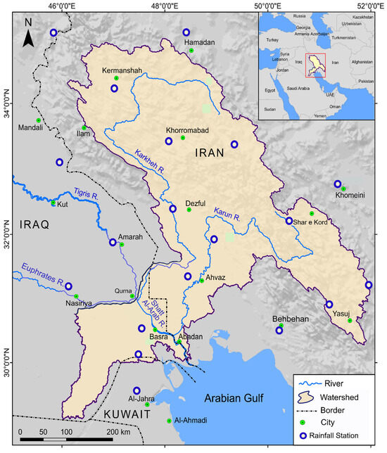
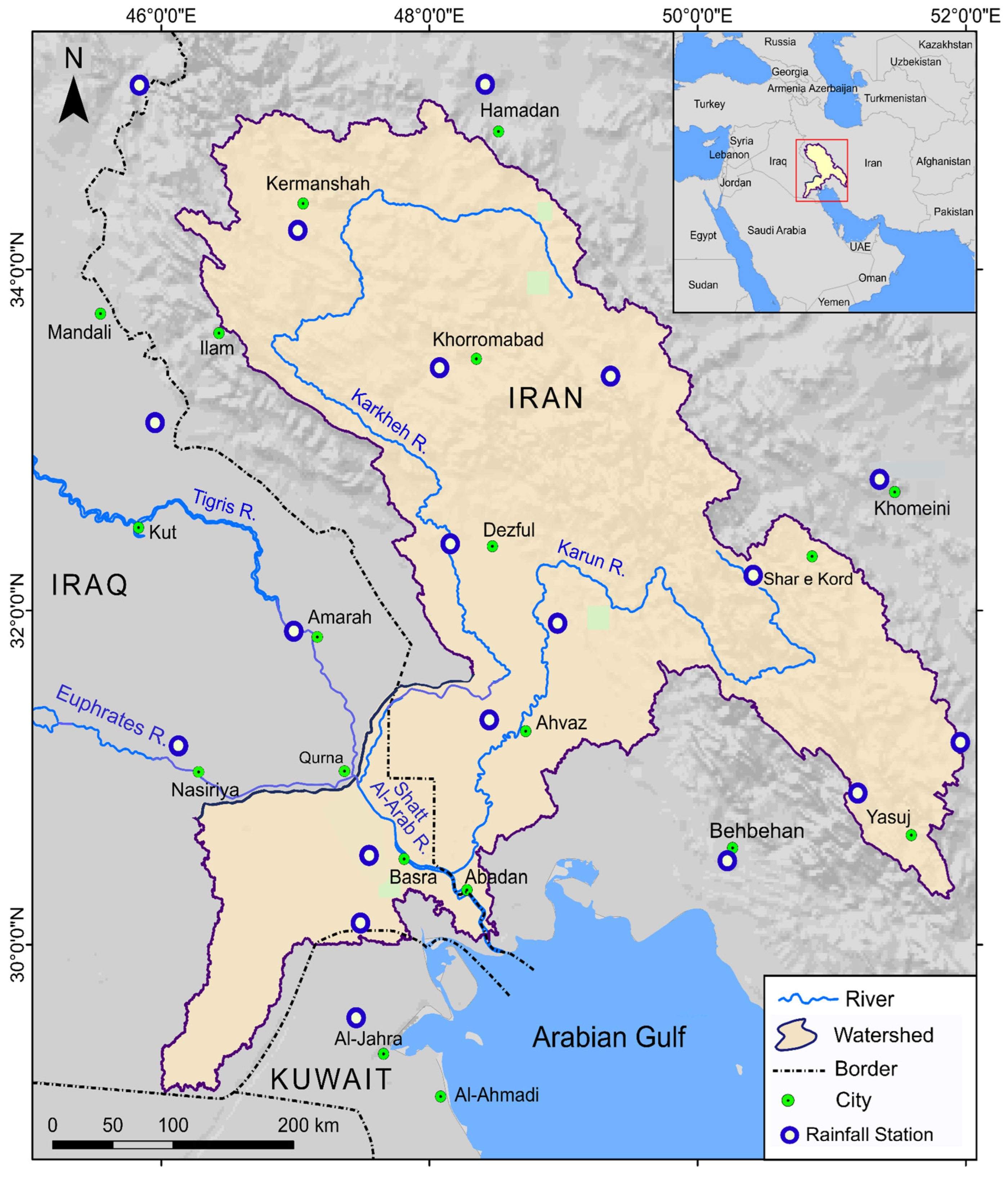
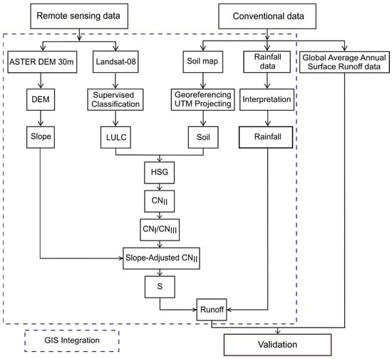
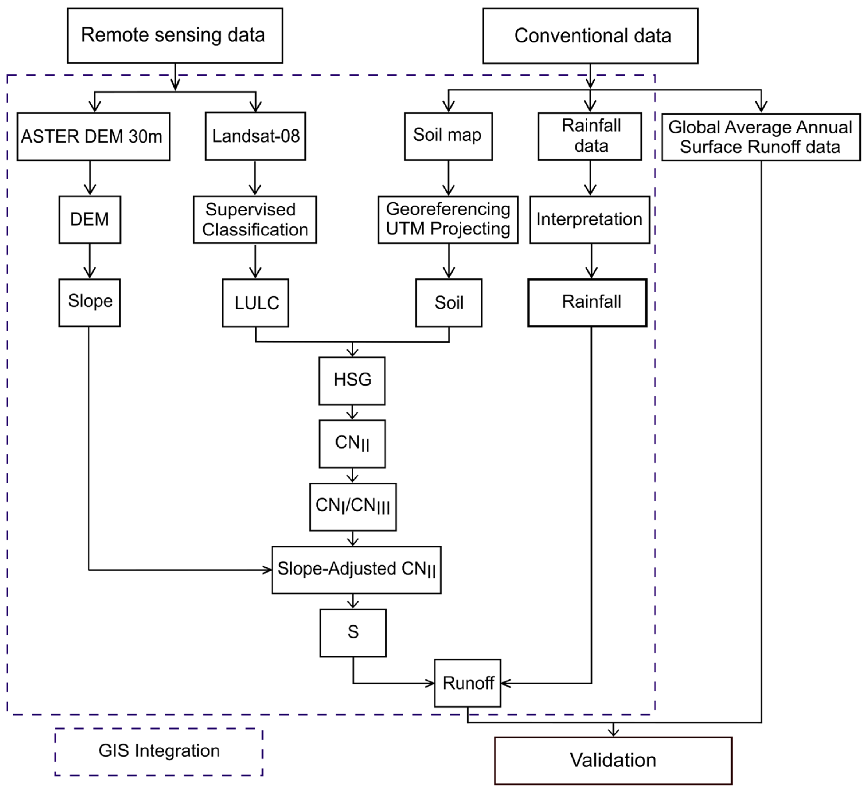
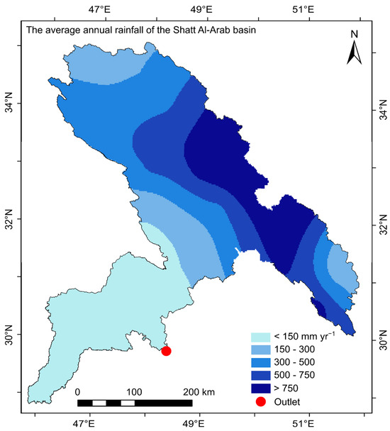
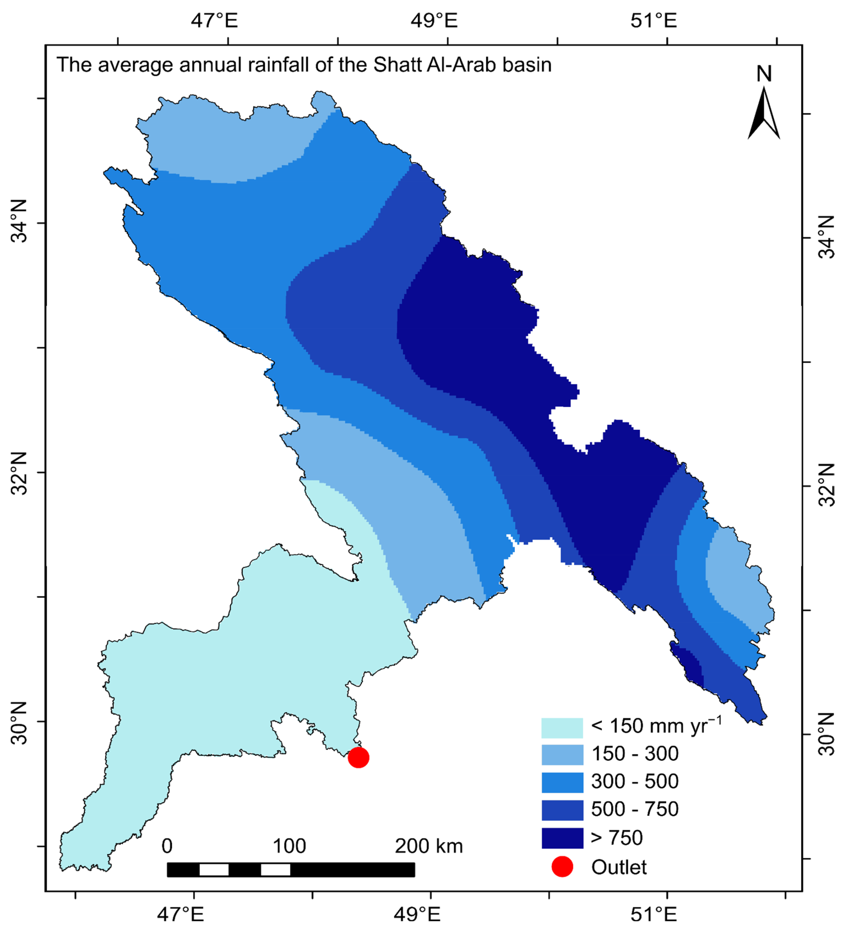
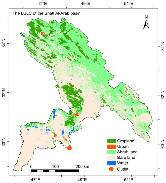
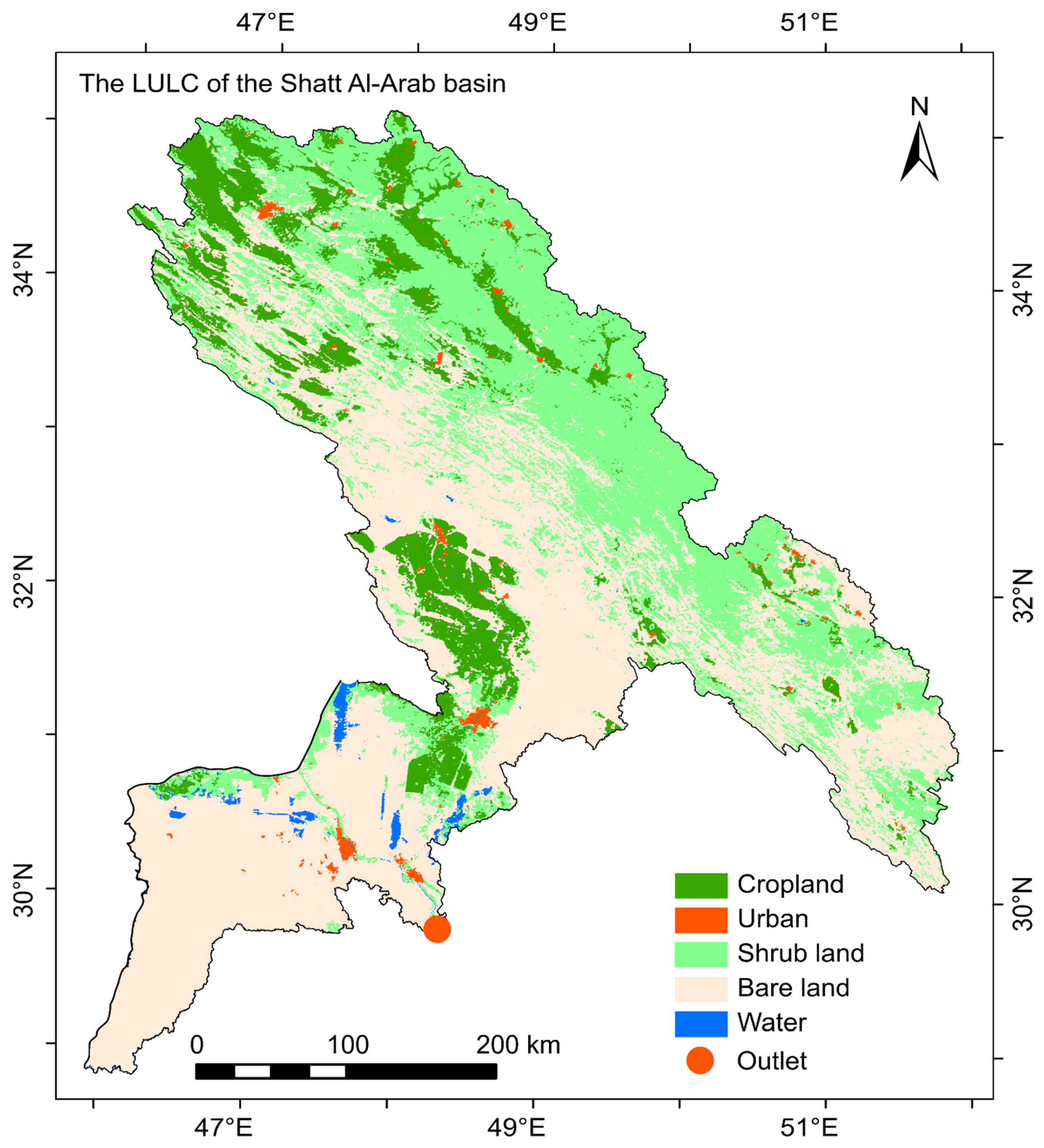
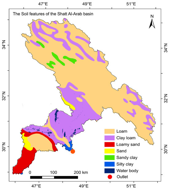
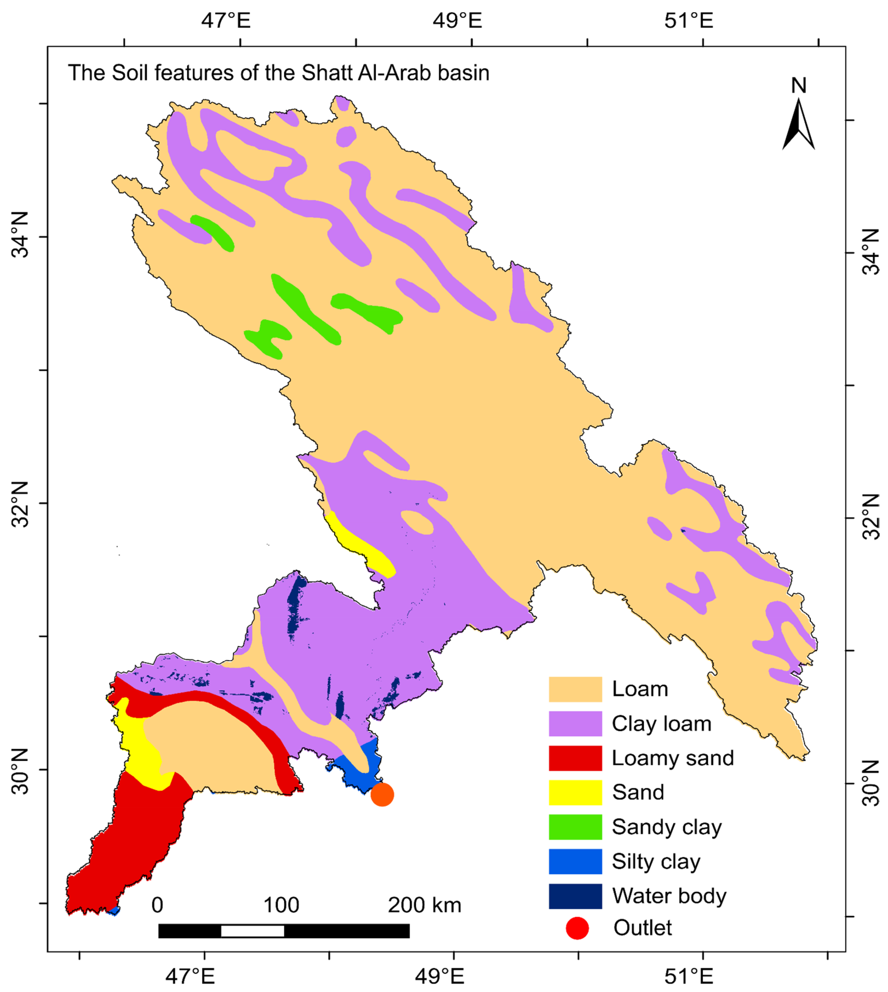
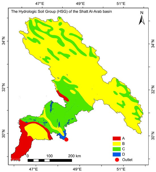
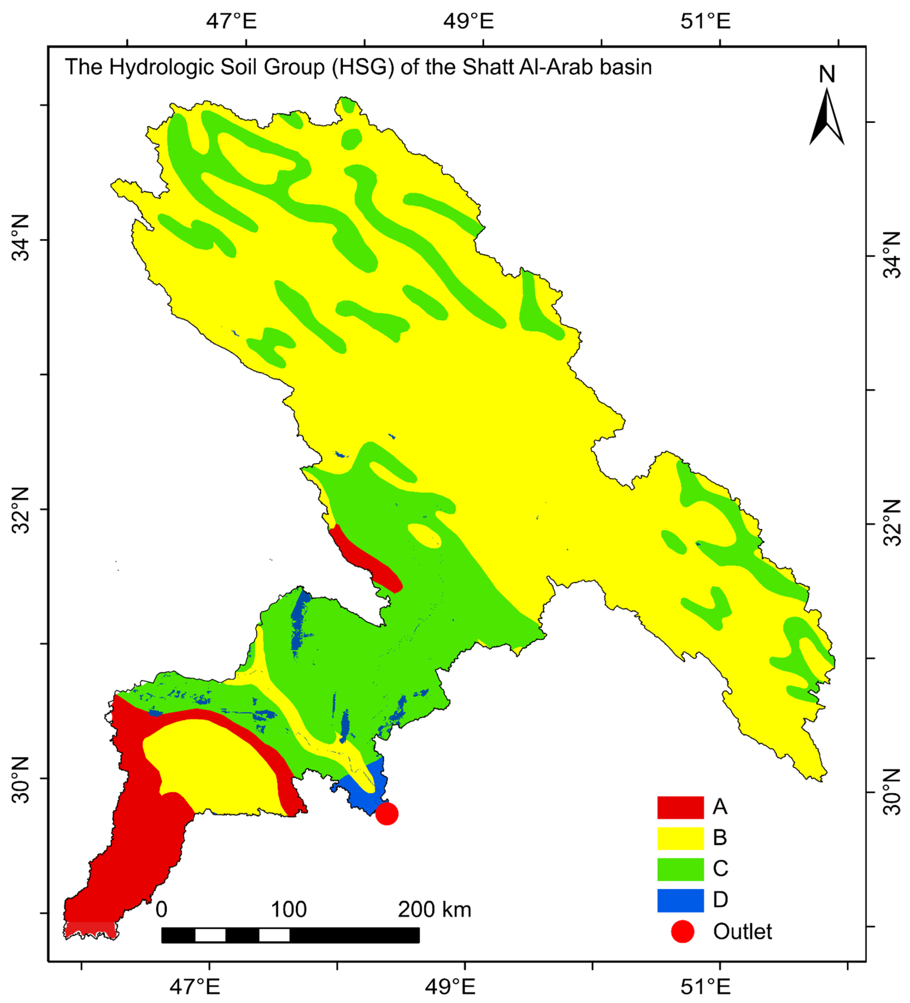
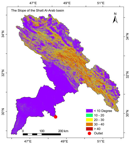
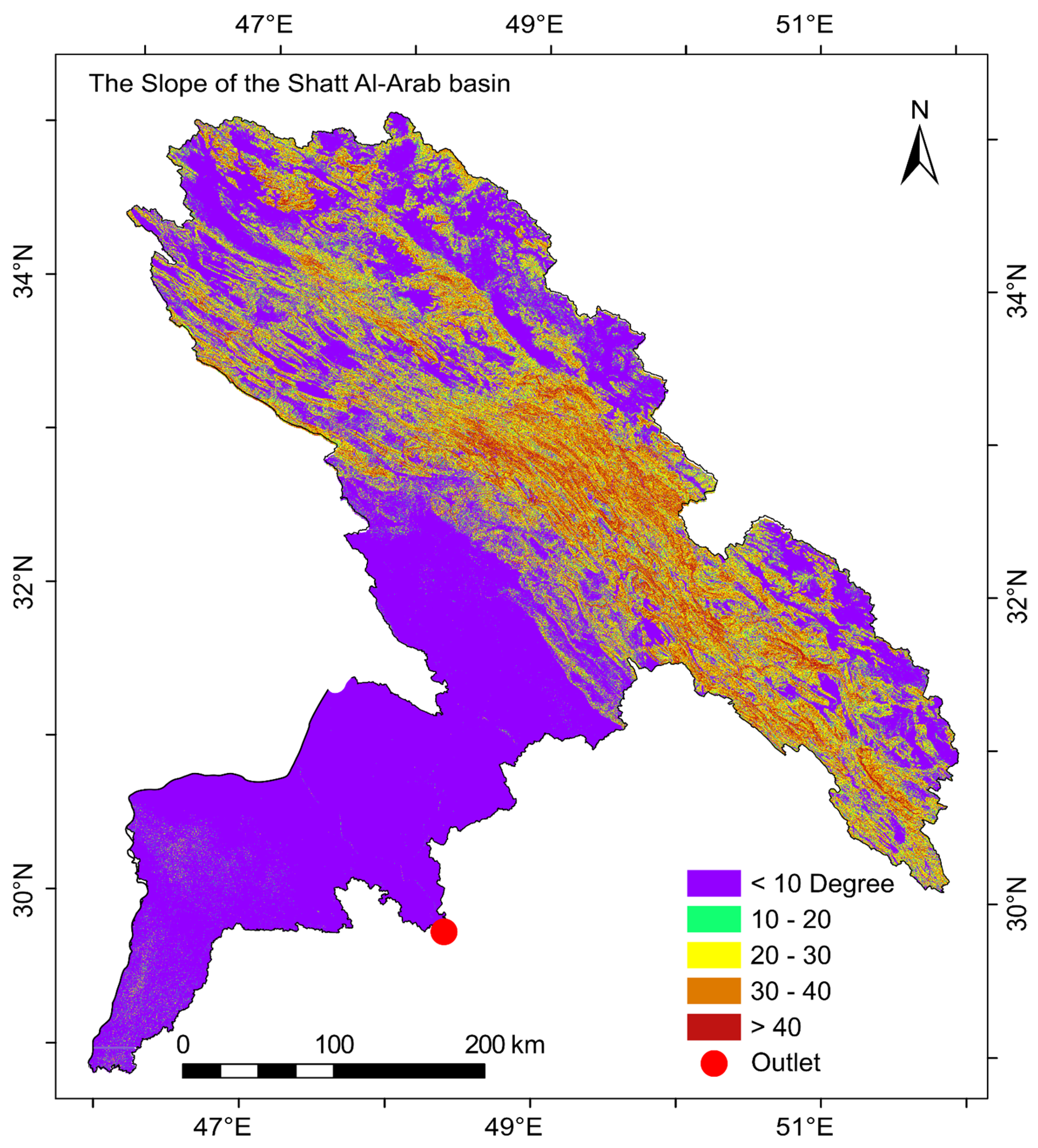
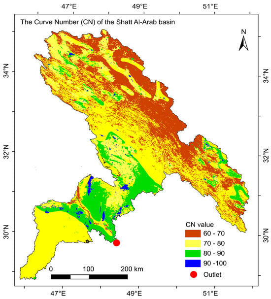
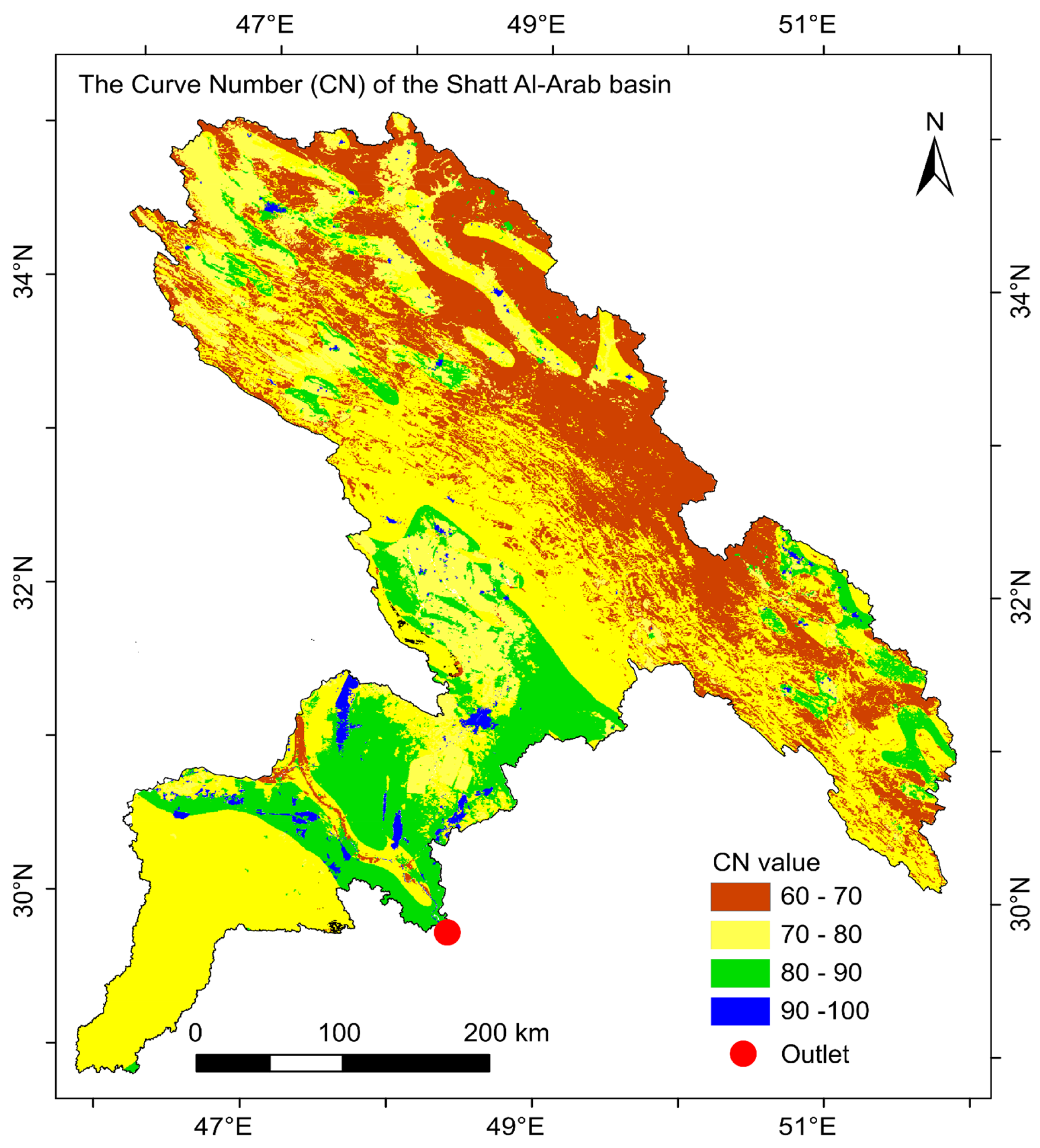
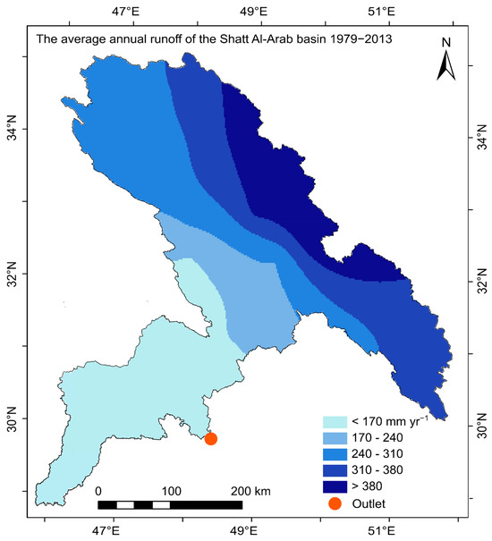
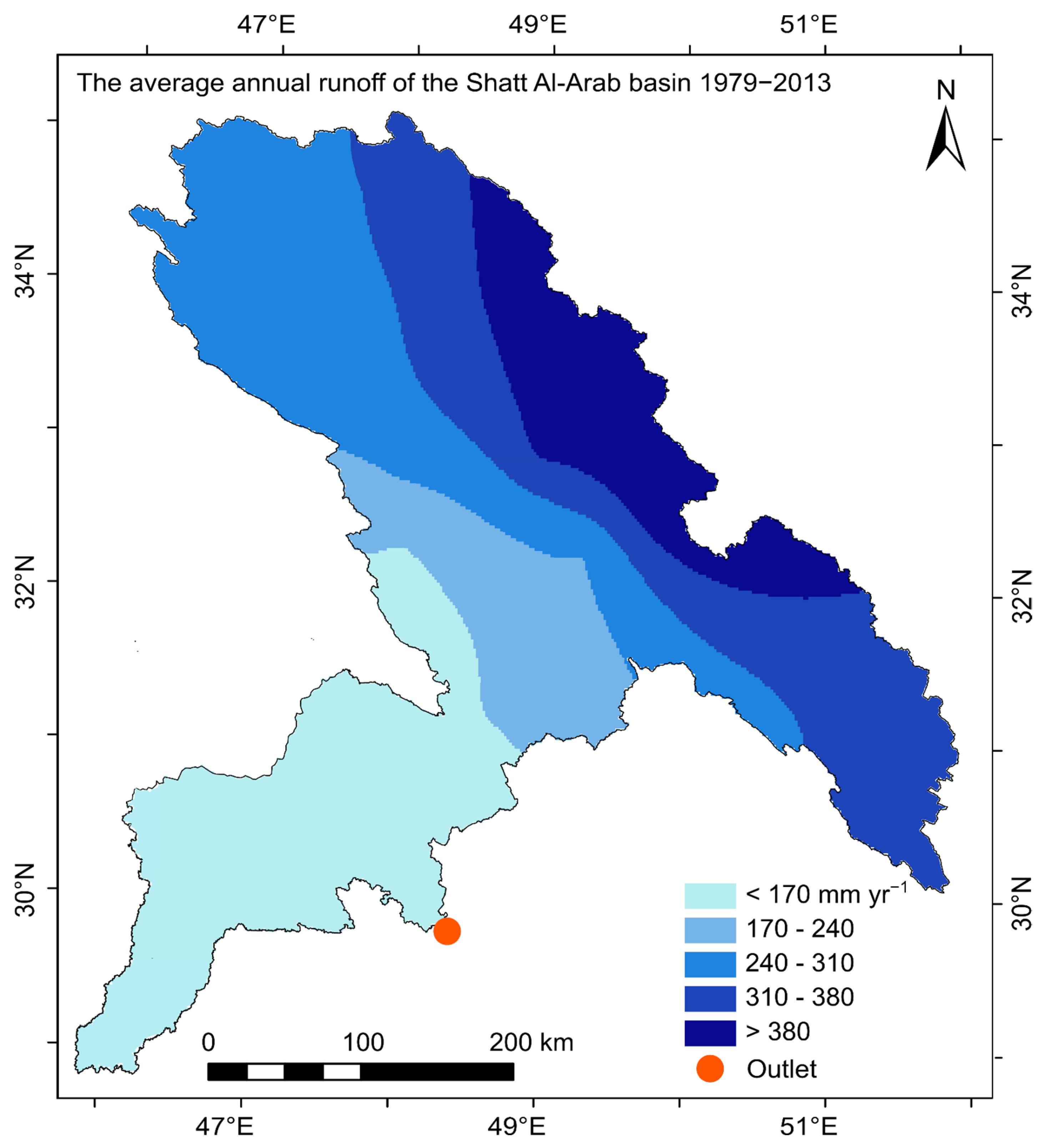
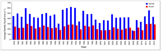
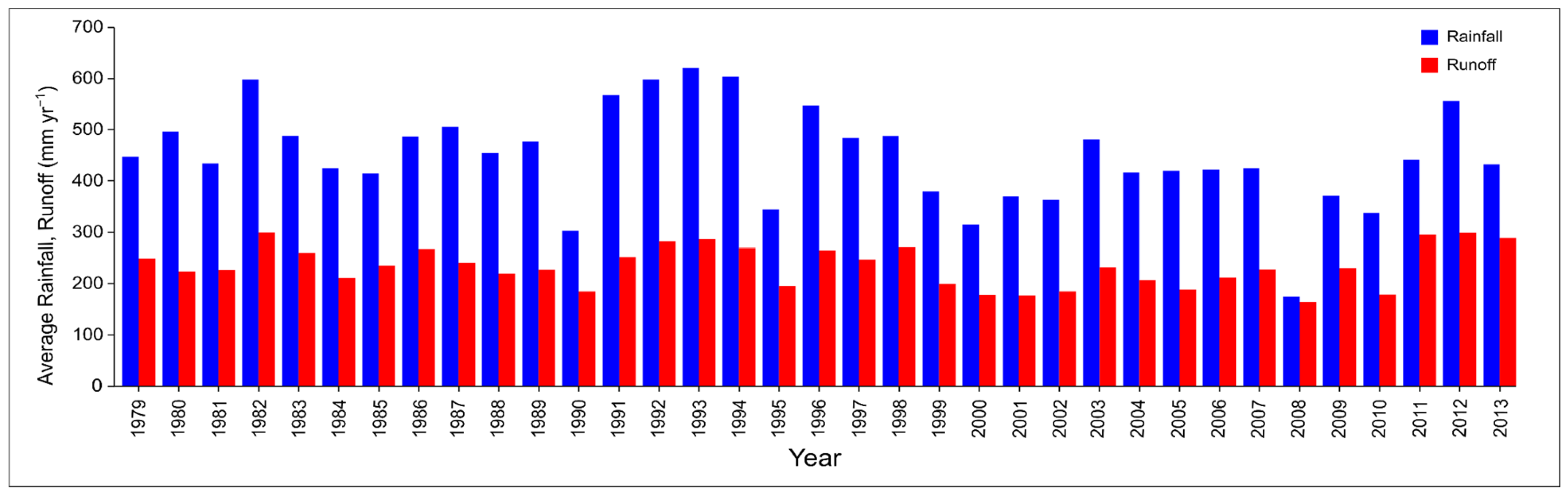
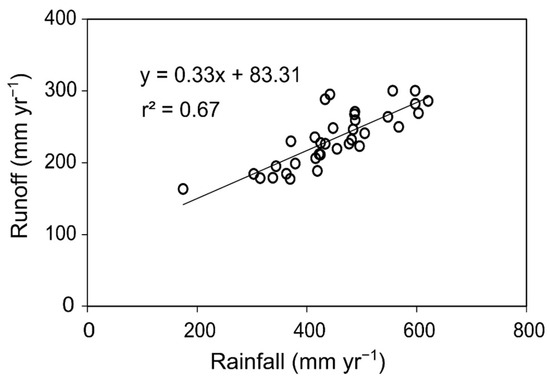
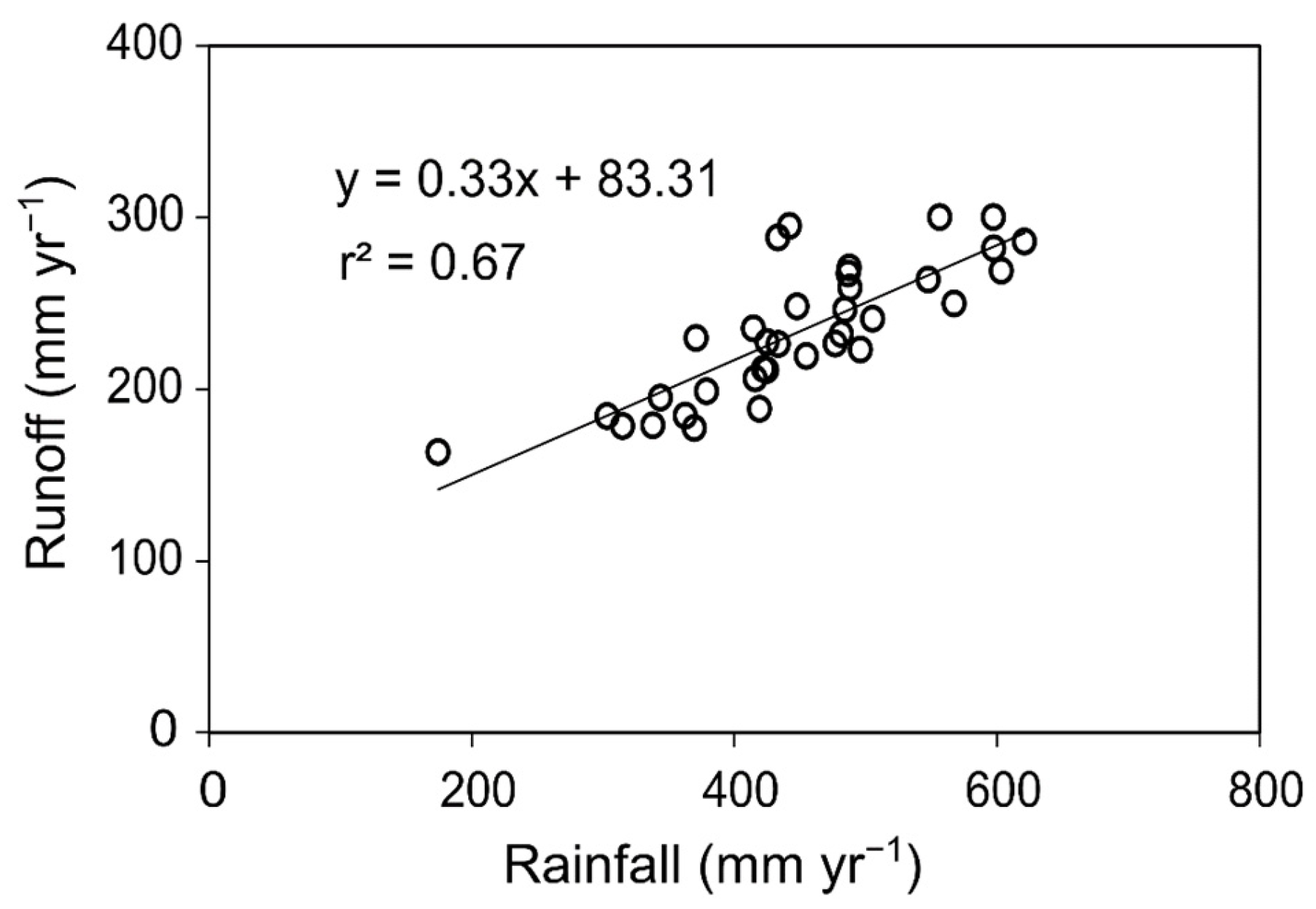
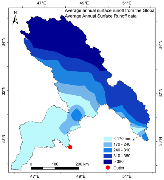
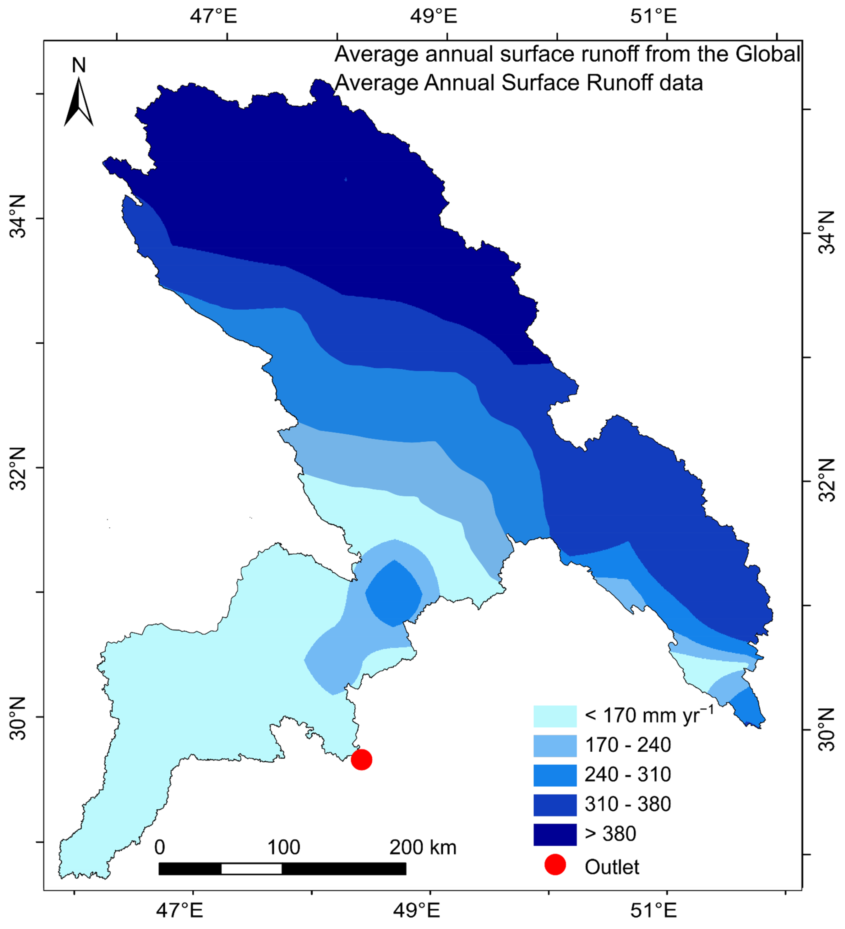
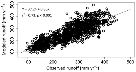
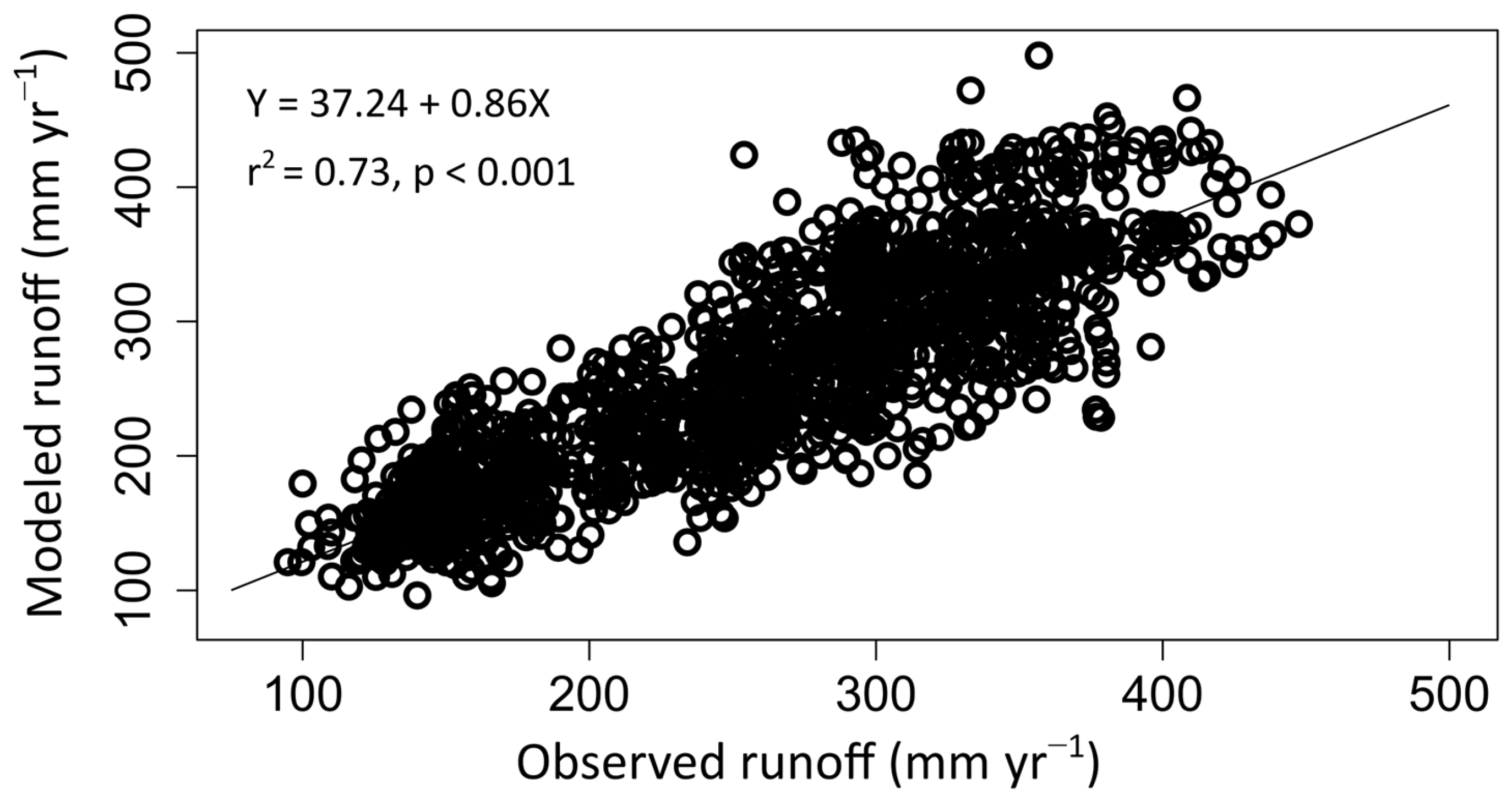

Disclaimer/Publisher’s Note: The statements, opinions and data contained in all publications are solely those of the individual author(s) and contributor(s) and not of MDPI and/or the editor(s). MDPI and/or the editor(s) disclaim responsibility for any injury to people or property resulting from any ideas, methods, instructions or products referred to in the content. |
© 2026 by the authors. Licensee MDPI, Basel, Switzerland. This article is an open access article distributed under the terms and conditions of the Creative Commons Attribution (CC BY) license.