Cross-Zonal Short-Term Load Forecasting in Resource-Constrained Distribution Grids: A Multi-Model Benchmarking Study

Abstract

Accurate short-term load forecasting is essential for modern power distribution, yet selecting optimal predictive architectures across diverse feeder profiles remains a key challenge for local grid operators. This paper presents a multi-feeder comparative evaluation of machine learning architectures using hourly load data (January 2024–April 2026) from six distribution feeders within two operational zones under the Bangladesh Rural Electrification Board. The evaluated models include statistical baselines (ARIMA, SARIMA), linear regression, tree ensembles (Random Forest, XGBoost, LightGBM), and recurrent architectures (LSTM, GRU). Feature engineering includes cyclical temporal encodings, weather parameters, and temporal lags. Experimental results demonstrate that tree-based ensembles consistently outperform both statistical baselines and recurrent neural networks across all feeders. Random Forest achieved the highest performance, with a Mean MAPE of 2.35%, and individual feeder errors reaching as low as 0.83% MAPE and 0.02 MW MAE. Meanwhile, LightGBM demonstrated superior operational deployment efficiency, delivering a highly comparable Mean MAPE of 2.56% with the lowest inference time of 0.55 s, and a minimal memory footprint of 1.2 MB. These findings highlight that feature-engineered tree ensembles provide an optimal balance of predictive performance, scalability, and computational efficiency for real-time distribution grid operations across neighboring utility zones.

1. Introduction

Load forecasting for electrical distribution substations is a foundational requirement for modern grid management. Precise short-term predictions allow utility providers to optimize power dispatch, prevent localized transformer overloads, and maintain regional grid stability [1]. Accurate short-term load forecasting (STLF) is especially vital when navigating unpredictable demand profiles in industrial-heavy feeders and supporting renewable energy integration [2].

To establish the operational scope of predictive modeling, load forecasting frameworks are traditionally categorized into four temporal horizons based on their engineering application [3]: Very Short-Term Load Forecasting (VSTLF) (minutes up to a day) for real-time market clearing and automatic generation control; Short-Term Load Forecasting (STLF) (24 h to 168 h) for day-ahead unit commitment, peak demand mitigation, and security analysis; Medium-Term Load Forecasting (MTLF) (one week to several months) for fuel procurement and maintenance scheduling; and Long-Term Load Forecasting (LTLF)(years to decades) for capital infrastructure investments.

In Bangladesh, distribution utilities face distinct operational constraints shaped by rapid industrial growth, urban expansion, and legacy data collection infrastructures [4].

The existing power forecasting literature in Bangladesh heavily focuses on aggregated, national-level grid predictions [5,6]. However, national models naturally smooth out localized volatility. Substation- and feeder-level forecasting requires a far more granular approach capable of capturing micro-climate variations and feeder-specific consumer behaviors that national-scale models are structurally unable to resolve.

Beyond Bangladesh, while feeder- and substation-level STLF has been explored globally using various machine learning algorithms [7,8,9], existing benchmarking studies suffer from two key limitations. First, most studies evaluate predictive models on isolated, single-feeder datasets, failing to assess cross-zonal generalizability across heterogeneous consumer profiles (e.g., highly volatile industrial feeders versus cyclical residential feeders). Second, conventional STLF research focuses almost exclusively on offline predictive error metrics (such as MAPE or RMSE) while completely neglecting edge-deployment hardware constraints—such as model memory footprints, training duration, and per-window inference latency. In resource-constrained distribution grids managed by rural electric cooperatives, selecting an optimal model requires evaluating the explicit trade-offs between predictive accuracy and real-time computational overhead.

To bridge these gaps, this paper presents a comprehensive multi-feeder benchmarking study utilizing high-resolution hourly load data collected directly from power loggers installed across six distribution feeders operating under the Bangladesh Rural Electrification Board (BREB). BREB distributes electricity through rural electric cooperatives called Palli Bidyut Samities (PBSs). We evaluate hourly data spanning from 1 January 2024 to 30 April 2026 across two major operating zones: Gazipur PBS-1 (Joydebpur-7 F5, Gacha-1 F4, Gacha-1 F3) and Mymensingh PBS-2 (Sreepur-1 F5, Sreepur-7 F1, Sreepur-8 F2).

Using a unified 43-feature matrix incorporating historical load lags, cyclical temporal encodings, and localized meteorological parameters (temperature, humidity, wind speed) extracted from the Open-Meteo API [10], we systematically evaluate eight forecasting models across a multi-window recursive 168 h (7-day) rolling horizon. The evaluated architectures span classical statistical baselines (ARIMA, SARIMA, linear regression), tree-based ensembles (Random Forest [11], XGBoost [12], LightGBM [13]), and recurrent deep neural networks (LSTM [14], GRU [15]).

This study makes four primary contributions:

• Cross-Zonal Multi-Feeder Benchmark: Establishing a realistic performance evaluation across six distribution feeders exhibiting starkly contrasting industrial and residential load profiles across two distinct utility zones (Gazipur PBS-1 and Mymensingh PBS-2).
• Unified Multi-Model Benchmarking: Rigorously comparing statistical baselines, gradient-boosted ensembles, and recurrent deep learning structures under an identical 168 h recursive rolling forecast horizon and identical 43-feature input representations.
• Domain-Specific Feature Integration: Quantifying the impact of localized meteorological dependencies (temperature, relative humidity, wind speed) and cyclical time encodings on capturing volatile feeder-level dynamics.
• Operational Deployment and Efficiency Analysis: Evaluating model viability beyond accuracy by measuring exact memory footprints, training execution times, and per-window batch inference latencies to determine optimal candidates for real-time edge integration into utility monitoring systems.

2. Related Work

Short-term load forecasting (STLF) at the distribution substation and feeder levels has evolved significantly from classical parametric formulations to non-linear data-driven architectures [2,7]. This section critically reviews the progression of STLF methodologies and synthesizes the existing literature regarding multi-feeder load dynamics, computational execution constraints, and cross-zonal generalizability.

2.1. Evolution of STLF Methodologies

Early STLF frameworks predominantly relied on linear regression and classical statistical formulations due to their analytical tractability [2]. While traditional parametric models effectively capture smooth periodic seasonal trends in aggregated grid demand, their linear structural assumptions limit performance when applied to lower-level distribution feeders characterized by high volatility, non-linear meteorology–demand interactions, and exogenous disruptions [7].

To overcome these non-linear constraints, machine learning (ML) algorithms gained prominence. Tree-based ensemble methods, such as Random Forest (RF) [11,16], non-parametrically map non-linear feature interactions. Subsequent advances in gradient-boosted decision trees (GBDTs)—specifically Extreme Gradient Boosting (XGBoost) [12] and Light Gradient Boosting Machine (LightGBM) [13]—demonstrated superior predictive performance on tabular grid telemetry [17]. LightGBM, in particular, utilizes leaf-wise tree growth and histogram-based feature binning, drastically reducing memory footprint and training overhead while maintaining robust performance across multi-step forecast horizons.

Concurrently, deep learning (DL) architectures have been extensively explored for sequence modeling. Recurrent neural network (RNN) variants, such as Long Short-Term Memory (LSTM) [6,14,18,19] and Gated Recurrent Units (GRU) [15,20], excel at capturing temporal dependencies without manual feature engineering. Hybrid structures combining convolutional feature extractors or attention mechanisms with recurrent layers have further enhanced predictive accuracy [5,8,21]. However, deep architectures introduce higher parameter counts and significant computational complexity during training and deployment.

2.2. Cross-Zonal Feeder Dynamics and Computational Overhead Gaps

Despite the extensive literature comparing algorithmic variations, existing STLF studies exhibit two major critical limitations:

First, the vast majority of STLF research evaluates model efficacy solely through offline predictive error metrics, such as RMSE, MAPE, and MAE [3,9]. Complex deep learning structures and large ensemble models are frequently declared optimal based on marginal reductions in error, without profiling operational execution overhead. In practical energy management systems (EMSs) and distribution management systems (DMSs), particularly at resource-constrained rural substations [4], hardware capabilities are strictly limited. Crucial operational parameters—such as disk storage footprint, offline retrain duration, and online batch inference latency per forecast window—are rarely benchmarked under unified, standardized hardware conditions.

Second, the existing literature heavily focuses on high-level transmission grid demand [1], aggregated macro-regions [22], and single-substation transformer datasets [23]. Distribution networks in developing power grids consist of highly heterogeneous feeder lines (e.g., dedicated industrial, mixed commercial–residential, or heavy agricultural zones) subject to severe ambient weather variations and operational disruptions. A forecasting model tuned for an aggregated region or single transformer often fails when deployed across adjacent, distinct feeder topographies. A comprehensive, standardized multi-model benchmarking framework evaluated across multi-feeder cross-zonal distribution topologies remains absent.

Beyond standalone predictive performance, high-precision feeder-level load forecasting serves as a critical foundational layer for downstream operational control, including dynamic demand-side management, optimal load dispatch, and smart microgrid scheduling [24].

To highlight these research gaps, Table 1 systematically compares representative STLF studies against the proposed benchmarking framework.

Table 1. Systematic comparison of representative short-term load forecasting studies against the proposed benchmarking framework.

Study	Model Spectrum Covered	Target Level/Scope	Multi-Feeder/ Cross-Zonal	Forecast Horizon (h)	Inference Latency Profiling	Hardware/Storage Footprint
Kong et al. [18]	Deep Learning (LSTM)	Residential Customers	No	1 h	No	No
Liu et al. [23]	Deep Learning	Transformer Level	No	24 h	No	No
Rafi et al. [5]	Deep Hybrid (CNN-LSTM)	System Level	No	24 h	No	No
Figueiró et al. [22]	Statistical/ML	Macro-Region	Limited	24 h	No	No
Magalhães et al. [16]	ML (Random Forest)	Substation Level	No	24 h	No	No
Shiblee & Koukaras [17]	GBDT & Deep Learning	Distribution System	No	24 h	Partial	No
Shahinzadeh et al. [25]	GBDT/Probabilistic	Distribution Grid	No	24 h	No	No
This Work	Classical, GBDT, & Deep Learning	Substation & Feeders	Yes (Cross-Zonal)	168 h (Recursive)	Yes (s/win)	Yes (MB/CPU)

3. Methodology

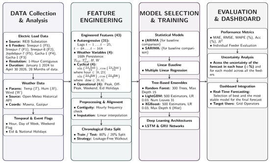
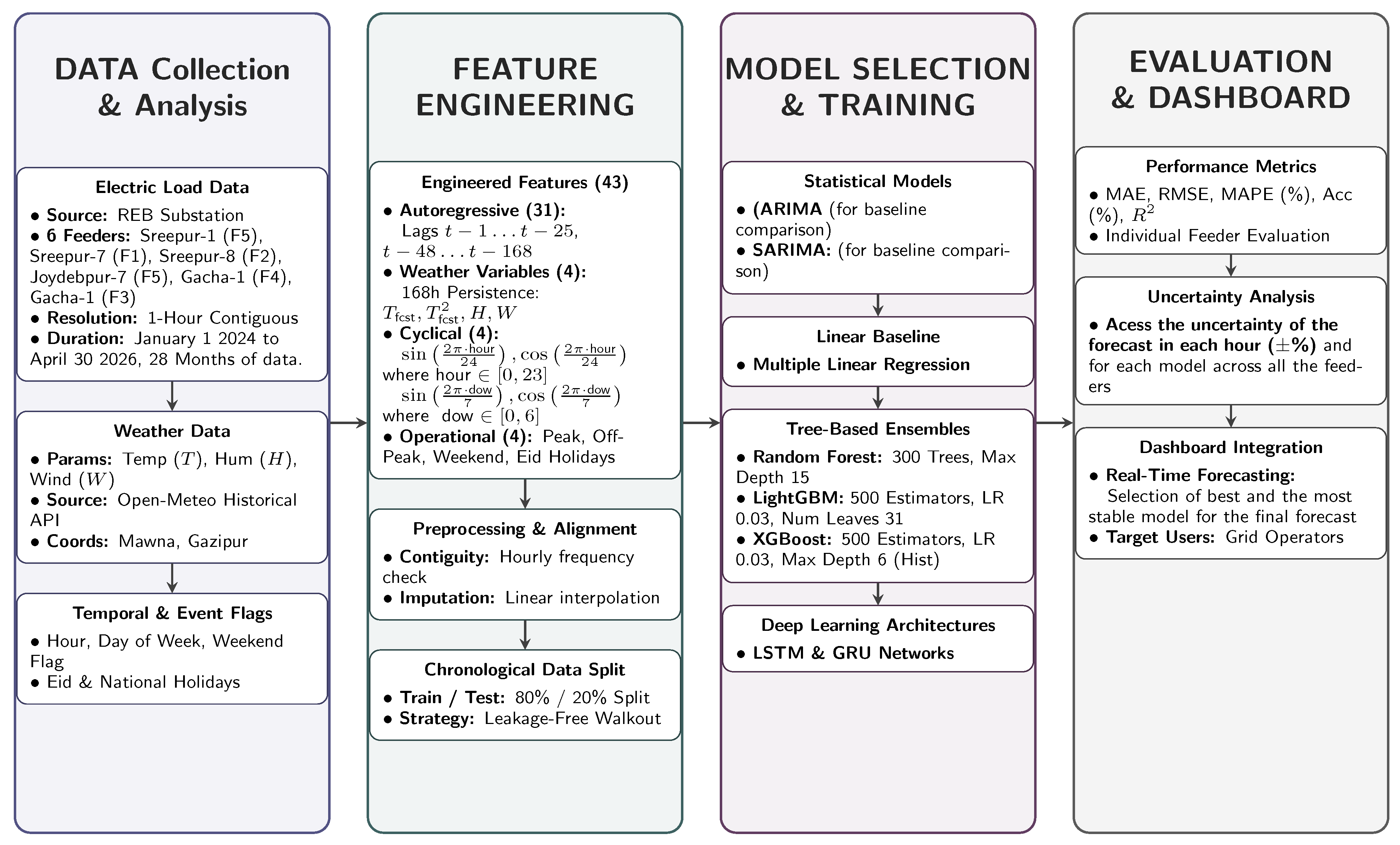
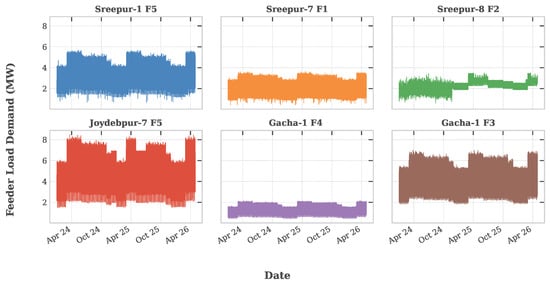
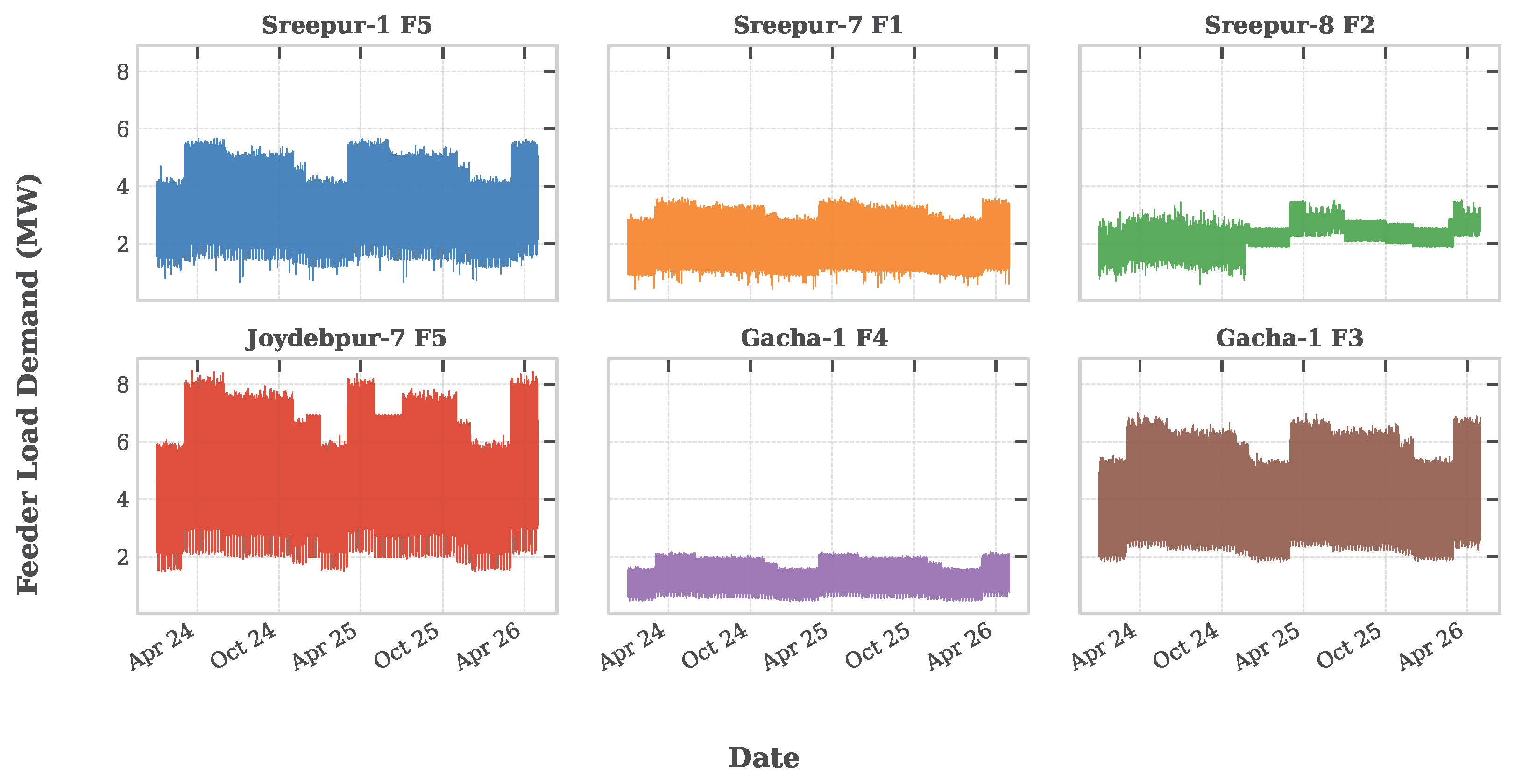
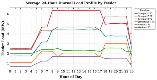
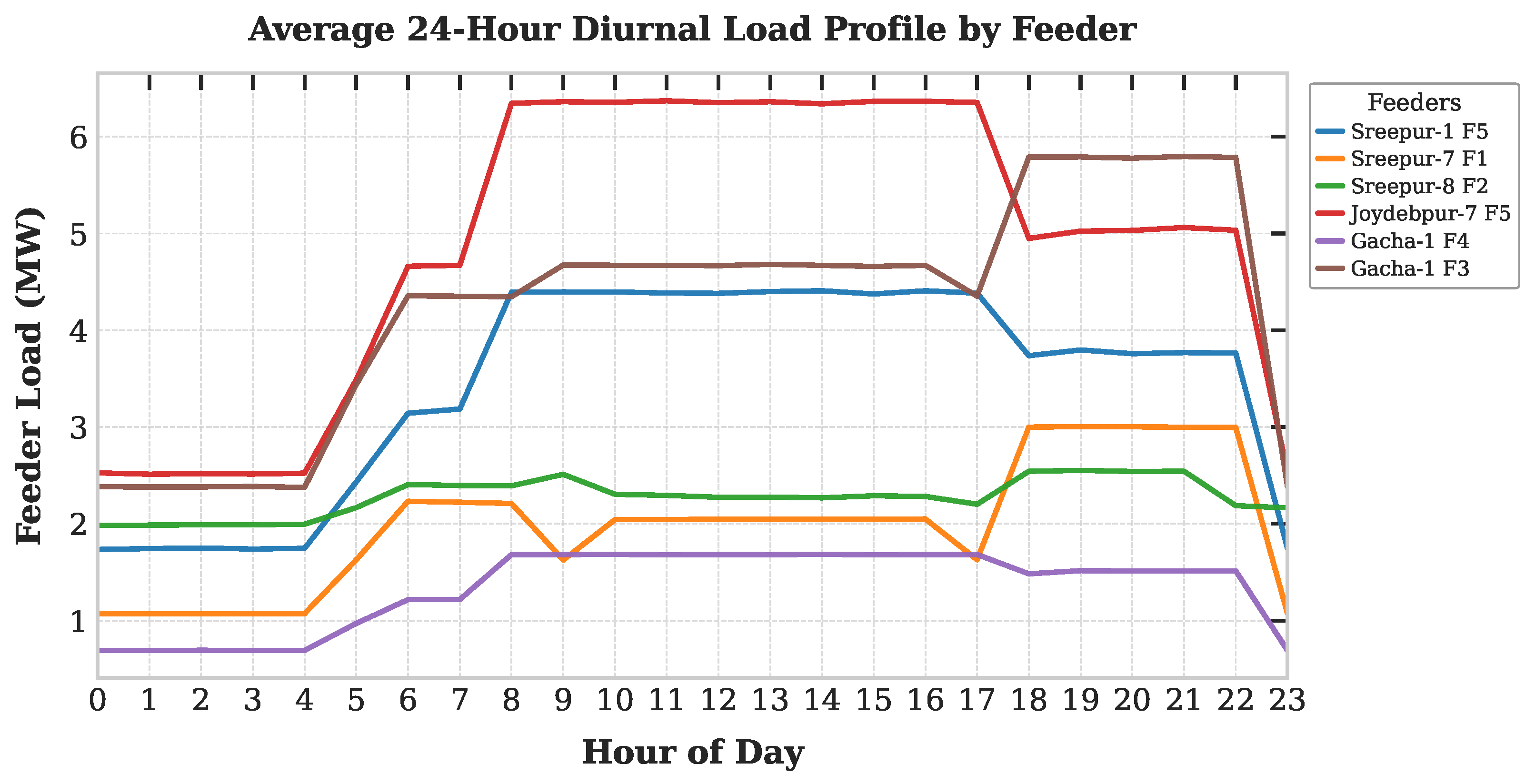
The overall end-to-end forecasting pipeline, spanning data ingestion through model deployment, is illustrated in Figure 1, while the long-term historical hourly load distributions and average 24 h diurnal consumption patterns across all six feeders are presented in Figure 2 and Figure 3, respectively.

Figure 1. Systematic workflow of the multi-feeder load forecasting framework: from raw feeder and weather acquisition (via substation power loggers), through 43-feature engineering, to individual model training, testing, and deployment.

Figure 2. Historical hourly load curves decomposed across individual distribution feeders in a $2\times 3$ grid panel, illustrating baseline load disparities, seasonal peak oscillations, and feeder-specific outages over the study period. Feeder subplots are color-coded for visual distinction.

Figure 3. Average 24 h diurnal load profiles across individual distribution feeders, highlighting distinct temporal consumption patterns and consumer heterogeneity across the distribution network.

3.1. Data Collection and Preprocessing

The load data is collected from the substation power loggers introduced in Section 1, one per feeder, across all six distribution feeders (Sreepur-1 F5, Sreepur-7 F1, Sreepur-8 F2, Joydebpur-7 F5, Gacha-1 F4, and Gacha-1 F3), spanning from 1 January 2024 to 30 April 2026.

Mathematical Scaling and Power Derivation: Each power logger records secondary-side electrical parameters (i.e., the low-voltage, low-current signals output by the substation’s instrument transformers) at high-frequency 5 min sampling intervals. To reconstruct true primary-side active power demand ($P_{\mathrm{primary}}$ in MW) from secondary-side readings ($P_{\mathrm{secondary}}$ in W), Potential Transformer ($K_{\mathrm{PT}}$) and Current Transformer ($K_{\mathrm{CT}}$) scaling multipliers were applied across all three phases, as follows:

$$P_{\mathrm{primary}}=P_{\mathrm{secondary}}\times K_{\mathrm{PT}}\times K_{\mathrm{CT}}$$

(1)

For instance, given secondary parameters $U_A=63.95\mathrm{V}$, $I_A=1.743\mathrm{A}$, and $P{F}_A=0.945$, the secondary active power $P_{A,\mathrm{secondary}}=105.39\mathrm{W}$ scales with transformation ratios $K_{\mathrm{PT}}=100$ and $K_{\mathrm{CT}}=100$ to yield $1.054\mathrm{MW}$ per phase, yielding a total three-phase primary load $P_{\mathrm{total}}\approx 3.006\mathrm{MW}$.

Data Quality Enhancement and Temporal Aggregation: Raw hardware logs exhibited operational anomalies due to instrument calibration drifts, telemetry dropouts, and line faults. Data preprocessing followed a rigorous cleaning workflow:

• Anomaly Removal: Unphysical negative power readings resulting from reverse-current sensor artifacts were removed and flagged as missing values.
• Outlier Filtering: Extreme value spikes exceeding physical feeder thermal limits were identified and removed using rolling z-score statistical thresholding ($\left|z\right|>3.5$).
• Imputation Strategy: Short contiguous missing values (≤3 consecutive hours) were imputed using linear interpolation, while larger structural gaps were resolved using same-hour profile mapping from identical days of preceding weeks.
• Resampling: The cleaned 5 min active power time-series was temporally averaged to an hourly frequency profile to match the target operational horizon for short-term load forecasting (STLF).

Across the entire dataset, negative values, outliers and missing observations accounted for under 1.2% of total records, as shown in Table 2. To evaluate the statistical behavior and dynamic properties of the multi-feeder load data, we conducted descriptive statistical profiling and stationarity analysis across all six distribution channels. Stationarity was evaluated using the Augmented Dickey–Fuller (ADF) test.

Table 2. Raw data collection, cleaning statistics ($z=3.5$), effective hours, and per-feeder missing ratios across the six BREB distribution feeders.

Feeder Name	Data Span	Freq.	Raw Records	Effective Hours	Zeros/Neg.	Outliers	Per-Feeder Missing (%)
Sreepur-1 F5	1 January 2024 to 30 April 2026	5 min	245,088	20,424	2316	413	1.11%
Sreepur-7 F1	1 January 2024 to 30 April 2026	5 min	245,088	20,424	2863	337	1.31%
Sreepur-8 F2	1 January 2024 to 30 April 2026	5 min	245,088	20,424	6986	249	2.95%
Joydebpur-7 F5	1 January 2024 to 30 April 2026	5 min	245,088	20,424	2062	435	1.02%
Gacha-1 F4	1 January 2024 to 30 April 2026	5 min	245,088	20,424	1070	679	0.71%
Gacha-1 F3	1 January 2024 to 30 April 2026	5 min	245,088	20,424	83	123	0.08%
Average/Total	All Feeders	5 min	1,470,528	122,544	13,894	2458	1.20% (Avg.)

3.2. Feature Engineering

To capture the key drivers of electrical demand, we constructed 43 features of four main categories, as summarized in Table 3. Here, autoregressive lags capture historical load patterns and daily cycles; weather variables account for temperature and humidity changes; cyclical features maintain smooth transitions across hours and days; and event flags account for weekends, holidays, and peak hours in which load changes. The empirical justification for these feature selections, including temporal lag structure and weather variable correlation analyses, is detailed in Section 4.2.

Table 3. Summary of engineered features.

Category	Count	Variables
Weather	4	Temp, Temp2, Relative Humidity, Wind Speed
Autoregressive	31	$L_{t-1\dots t-25}$, $L_{t-48}$, $L_{t-72}$, $L_{t-96}$, $L_{t-120}$, $L_{t-144}$, $L_{t-168}$
Cyclical	4	$\sin \left({\displaystyle \frac{2\pi ·\mathrm{hour}}{24}}\right)$, $\cos \left({\displaystyle \frac{2\pi ·\mathrm{hour}}{24}}\right)$, $\sin \left({\displaystyle \frac{2\pi ·\mathrm{dow}}{7}}\right)$, $\cos \left({\displaystyle \frac{2\pi ·\mathrm{dow}}{7}}\right)$
Events	4	Eid Vacation, Peak, Off-Peak, Weekend
Total	43

During the 168 h rolling forecasting evaluation, weather variables (temperature, relative humidity, and wind speed) are generated without look-ahead bias by employing a 168 h historical persistence proxy. For each step $t+\tau$ within the horizon, weather values are derived from observations exactly 168 h prior ($t+\tau -168$). This ensures future weather ground truth is strictly excluded, preventing look-ahead bias.

3.3. Data Partitioning

To eliminate look-ahead bias and data leakage, all dataset boundaries were split chronologically using an 80/20 ratio, spanning the total study period from 1 January 2024 to 30 April 2026 (20,424 h). Specifically, the initial 80% (covering 1 January 2024 to 12 November 2025) was reserved for model training, and the final unseen 20% (covering 13 November 2025 to 30 April 2026) was held out as an unseen test set for multi-step recursive evaluation across 1 to 168 h look-ahead horizons. For the deep learning models, LSTM and GRU, we created a validation set from 10% of the training set to prevent overfitting by using early stopping. So, for the LSTM and GRU models, the data partition is 72% training, 8% validation, and 20% testing.

3.4. Model Training and Evaluation Framework

We benchmarked eight predictive models across four architectural paradigms: classical statistical baselines, linear regression, gradient-boosted/bagged tree ensembles, and recurrent deep neural networks.

3.4.1. Phase I: Statistical Baselines and Linear Regression

Classical statistical baselines (ARIMA, SARIMA, and linear regression) were configured via the statsmodels framework with rigorous, empirically justified specifications. For ARIMA, parameters $(p,q)$ were tuned per feeder using Akaike Information Criterion (AIC) minimization over a localized 672 h validation sample (corresponding to the final 4 weeks of the training split), with the differencing order d set from ADF tests ($d=1$ for Sreepur-8 F2; $d=0$ elsewhere). This yielded tailored specifications: $\mathrm{ARIMA}(2,0,2)$ for Sreepur-1 F5 and Gacha-1 F4; $\mathrm{ARIMA}(3,0,1)$ for Sreepur-7 F1; $\mathrm{ARIMA}(3,1,2)$ for Sreepur-8 F2; and $\mathrm{ARIMA}(3,0,2)$ for Joydebpur-7 F5 and Gacha-1 F3.

For SARIMA, unconstrained grid searches were avoided due to the computational cost of fitting seasonal models across multiple distribution feeders. Instead, configurations were evaluated over a targeted candidate set of the following four parsimonious structures:

(1)

$\mathrm{SARIMA}(1,0,0)\times {(1,1,0)}_{24}$ (Fast pure AR daily model);

(2)

$\mathrm{SARIMA}(2,0,0)\times {(1,1,0)}_{24}$ (Extended AR model);

(3)

$\mathrm{SARIMA}(1,0,1)\times {(1,1,0)}_{24}$ (Mixed non-seasonal ARMA model); 

(4)

$\mathrm{SARIMA}(1,0,0)\times {(0,1,1)}_{24}$ (Seasonal moving-average model).

All candidates incorporated $s=24$ with first-order seasonal differencing ($D=1$). AIC selection on the validation sample consistently identified $\mathrm{SARIMA}(1,0,0)\times {(0,1,1)}_{24}$ as the optimal model across all channels. Additionally, linear regression was evaluated using the full 43-variable feature matrix to establish a benchmark on the linear regression model.

3.4.2. Phase II: Tree-Based Ensemble Models

To model non-linear interactions and high-dimensional feature dependencies, three tree ensemble architectures were trained:

• Random Forest: A bagging ensemble constructed with 300 decision trees (maximum depth of 15), in line with empirical findings in STLF [16], as setting the estimator count to 300 stabilizes prediction variance while mitigating overfitting.
• LightGBM: A gradient-boosted decision tree model trained using Mean Squared Error (MSE) loss with 500 estimators, a learning rate of 0.03, and leaf-wise tree growth (num_leaves = 31) for optimal execution speed.
• XGBoost: A gradient-boosted decision tree model trained using MSE loss with 500 estimators, a learning rate of 0.03, a maximum tree depth of 6, and a histogram-based split method (tree_method = ‘hist’).

3.4.3. Phase III: Recurrent Deep Learning Networks

Recurrent neural networks (LSTM and GRU) were constructed to process 3D sequential feature tensors across a 24 h historical look-back window ($W=24$) with 43 input features. Both networks share a stacked two-layer architecture (64 and 32 hidden units) followed by a 16-unit dense layer (ReLU activation), utilizing a $20\%$ dropout rate after each recurrent layer to mitigate overfitting. Feature data and target variables were normalized using MinMaxScaler ($[0,1]$). Model optimization was conducted using the Adam optimizer ($\eta =0.001$) with Mean Squared Error (MSE) loss. Training was executed with a batch size of 32 for up to 50 epochs, incorporating an early stopping callback (patience = 7 epochs) based on 10% held-out validation loss to prevent overtraining and restore optimal model weights.

3.4.4. Computational Environment and Experimental Setup

All the training and experiments were executed within a standardized cloud-based Google Colab Linux environment.

The hardware and software specifications utilized for all benchmarking measurements are detailed as follows:

• Hardware Configuration: Operating within Google Colab’s standard cloud compute tier, the execution backend featured 2 logical vCPUs (1 socket, 1 core per socket, and 2 threads per core, with NUMA node 0 bound to CPUs $0,1$) and $12.67\mathrm{GB}$ of total system RAM.
• Operating System: Google Colab backend Linux kernel version 6.6.122+-x86_64 with GNU C Library (glibc) version 2.39.
• Software and Library Ecosystem: Built on Python version 3.13.16, incorporating key scientific and machine learning frameworks: statsmodels (0.15.0) for statistical baselines, Scikit-Learn (1.6.1) for regression benchmarks, XGBoost (3.4.1) and LightGBM (4.6.0) for gradient-boosted models, and TensorFlow (2.21.0) for deep learning architectures.

To rigorously evaluate model generalizability and identify the most suitable architecture for deployment in resource-constrained distribution substations (such as BREB), the evaluation followed a structured four-stage experimental protocol across the unseen 20% test split (spanning 13 November 2025 to 30 April 2026 across all six BREB feeders):

• Initial 1-Step-Ahead Screening: All eight candidate models were initially screened across 1-step-ahead test forecasts to filter out underperforming architectures.
• Multi-Step Recursive Evaluation: The top-performing architectures were advanced to a 168 h (7-day) recursive rolling multi-step forecasting evaluation across 24 forecast windows (comprising 4032 total forecast instances per model) on test data to simulate real-world operational lead times and quantify autoregressive error accumulation over extended horizons.
• Comparative Statistical Validation: The surviving models were subjected to rigorous comparative performance metrics (MAE, RMSE, MAPE, $R^2$) alongside Diebold–Mariano (DM) and Wilcoxon signed-rank significance tests to evaluate predictive superiority over the naive lag-168 h persistence model.
• Deployment Feasibility Selection: The final model selection balances predictive accuracy with computational efficiency.

4. Results

4.1. Feeder-Wise Statistical and Stationarity Profiling

As summarized in Table 4, each feeder records 20,424 hourly observations spanning from 1 January 2024 to 30 April 2026. Demand magnitude and volatility vary significantly across the six distribution channels. Mean load ranges from $1.3297\mathrm{MW}$ (Gacha-1 F4) to $4.8591\mathrm{MW}$ (Joydebpur-7 F5), with standard deviations highlighting high dynamic dispersion on Joydebpur-7 F5 ($1.7964\mathrm{MW}$) and Sreepur-1 F5 ($1.2127\mathrm{MW}$). Base loads range between $0.4338\mathrm{MW}$ and $1.8214\mathrm{MW}$, while peak demand reaches $8.4865\mathrm{MW}$ on Joydebpur-7 F5, underscoring capacity scale differences across rural and industrial circuits.

Table 4. Statistical properties across the six BREB distribution feeders.

Property	Sreepur-1 F5	Sreepur-7 F1	Sreepur-8 F2	Joydebpur-7 F5	Gacha-1 F4	Gacha-1 F3
Study Period (Start)	1 January 2024	1 January 2024	1 January 2024	1 January 2024	1 January 2024	1 January 2024
Study Period (End)	30 April 2026	30 April 2026	30 April 2026	30 April 2026	30 April 2026	30 April 2026
Total Data Points	20,424	20,424	20,424	20,424	20,424	20,424
Mean Load (MW)	3.4156	1.9709	2.2725	4.8591	1.3297	4.2268
Median Load (MW)	3.6076	1.9834	2.2815	5.1287	1.4152	4.5102
Mode Load (MW)	1.6640	1.0876	2.4905	2.7205	0.7604	2.4678
Standard Deviation (MW)	1.2127	0.6979	0.4302	1.7964	0.4593	1.2813
Variance	1.4705	0.4871	0.1851	3.2272	0.2110	1.6418
Minimum Load/Base Load (MW)	0.6769	0.4338	0.5993	1.4839	0.4429	1.8214
Maximum Load/Peak Demand (MW)	5.6581	3.6347	3.5093	8.4865	2.1480	6.9938
Skewness	−0.1998	0.2472	−0.0218	−0.0215	−0.2439	−0.2200
Kurtosis	−1.1588	−0.8068	0.0585	−1.1197	−1.1861	−0.9415
ADF Statistic	−13.3338	−6.1705	−2.8232	−16.4480	−13.7921	−6.4952
p-value	$6.1093\times {10}^{-25}$	$6.8237\times {10}^{-8}$	0.0550	$2.3931\times {10}^{-29}$	$8.8867\times {10}^{-26}$	$1.1993\times {10}^{-8}$
Stationarity	Stationary	Stationary	Non-Stationary	Stationary	Stationary	Stationary
	($p<0.05$)	($p<0.05$)	($p\ge 0.05$)	($p<0.05$)	($p<0.05$)	($p<0.05$)

Distributional metrics indicate predominantly left-skewed load profiles (skewness from $-0.0215$ to $-0.2439$) due to sustained commercial operation, except for Sreepur-7 F1 ($+0.2472$). The negative kurtosis across most channels reflects platykurtic distributions shaped by structured diurnal switching rather than extreme random spikes.

Augmented Dickey–Fuller (ADF) tests confirm that the five feeders strictly reject the unit-root null hypothesis ($p<0.05$), establishing statistical stationarity. Sreepur-8 F2 exhibits weak non-stationarity ($p=0.0550$), indicating localized trend dynamics that justify first-order differencing ($d=1$) for classical baseline models on this channel.

4.2. Feature Correlation Analysis

To empirically validate the drivers of electrical demand across the distribution grid, we examined the effects of lag features using ACF, weather variables (temperature, humidity, and wind) and their correlation with load, alongside calendar dynamics.

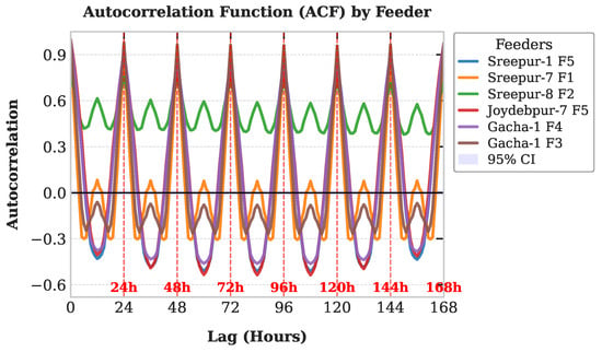
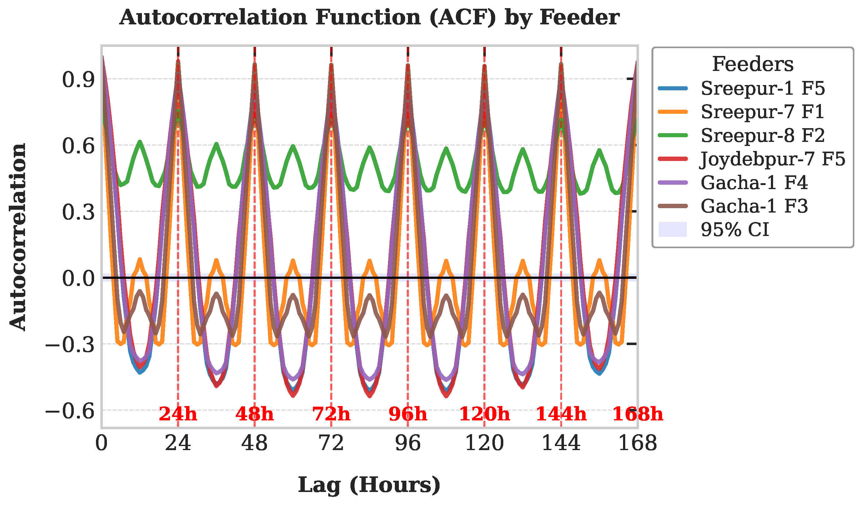
Autocorrelation Function (ACF) analysis (Figure 4) shows that pronounced peaks occur at 24 h intervals ($24n$), confirming strong daily seasonality across all feeder profiles. These findings validate our construction of the 31-variable autoregressive feature block, comprising the first 25 consecutive hourly lags ($L_1$ to $L_{25}$) alongside weekly seasonal lags ($L_{48}$, $L_{72}$, $L_{96}$, $L_{120}$, $L_{144}$, and $L_{168}$).

Figure 4. Autocorrelation Function (ACF) up to 168 h (7-day) lags across individual distribution feeders. Vertical dashed red lines highlight strong 24 h diurnal and weekly periodicity across all feeder channels.

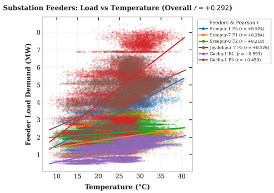
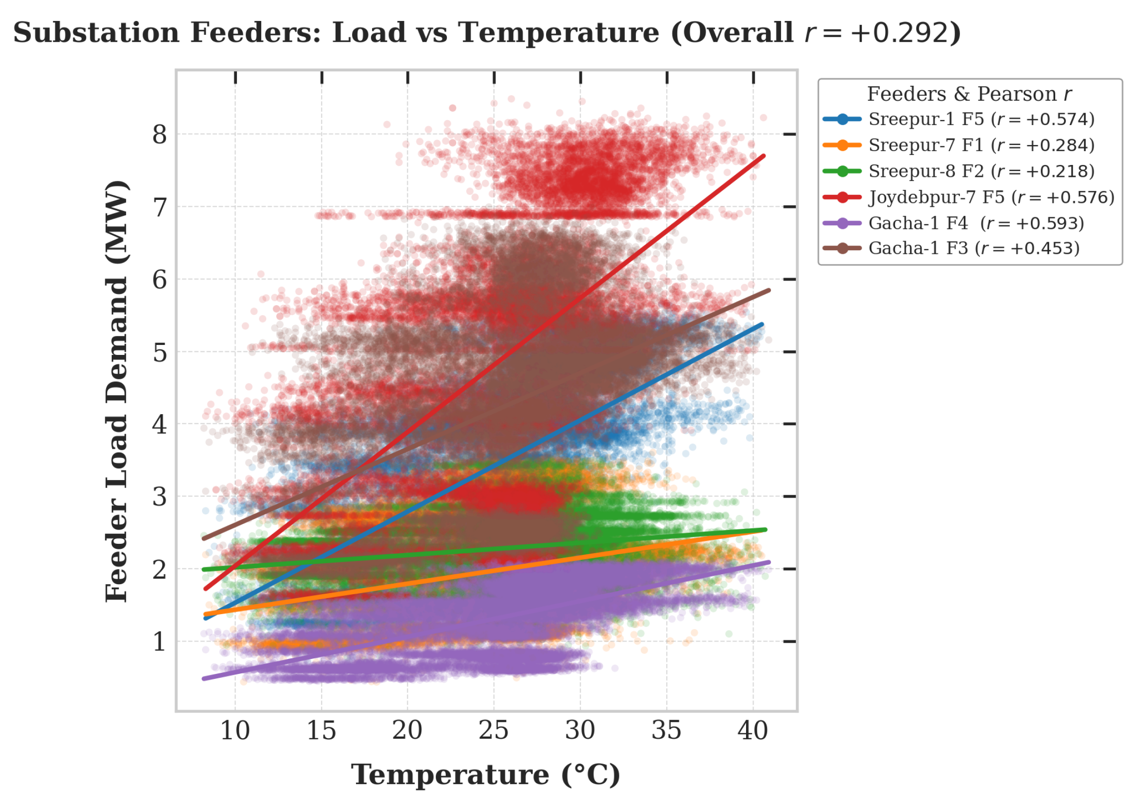
Temperature displays a positive overall correlation ($r=+0.292$) with electrical demand due to increased cooling loads during high-temperature intervals (Figure 5). Thermal sensitivity varies across individual channels: Gacha-1 F4 ($r=+0.593$), Joydebpur-7 F5 ($r=+0.576$), and Sreepur-1 F5 ($r=+0.574$) exhibit pronounced temperature dependencies, whereas Sreepur-8 F2 displays more moderate sensitivity ($r=+0.218$). These quantitative findings justify the inclusion of raw ambient temperature and the non-linear squared term ($T^2$) in our feature space.

Figure 5. Multi-feeder correlation analysis between hourly ambient temperature and demand. Fitted linear regression trends illustrate distinct temperature sensitivities across individual feeders (overall $r=+0.292$).

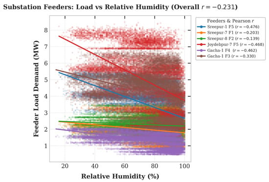
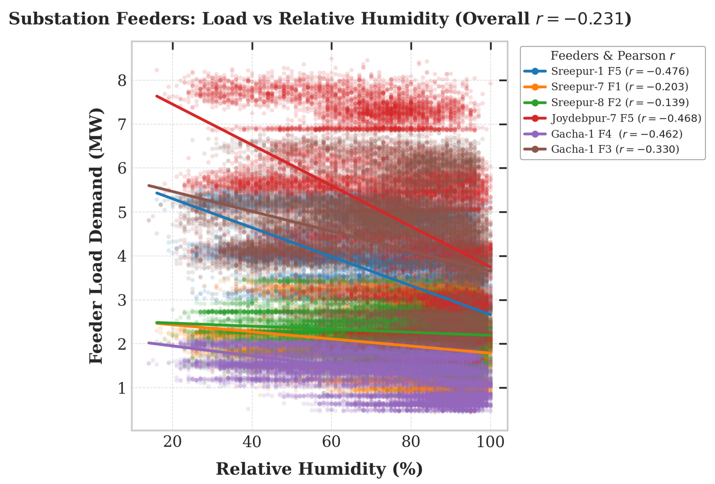
As illustrated in Figure 6, relative humidity exhibits an overall negative correlation with aggregate demand ($r=-0.231$), which is particularly strong on Sreepur-1 F5 ($r=-0.476$) and Joydebpur-7 F5 ($r=-0.468$). Peak humidity thresholds (95–100%) heavily coincide with monsoon precipitation and cloud cover, suppressing cooling load demand.

Figure 6. Multi-feeder correlation analysis between relative humidity and demand, showing localized negative correlation trends across distribution feeders ($r=-0.231$).

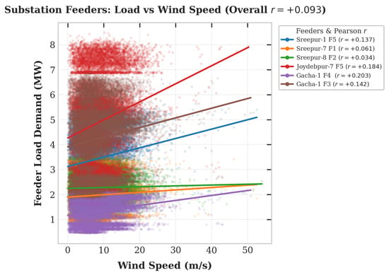
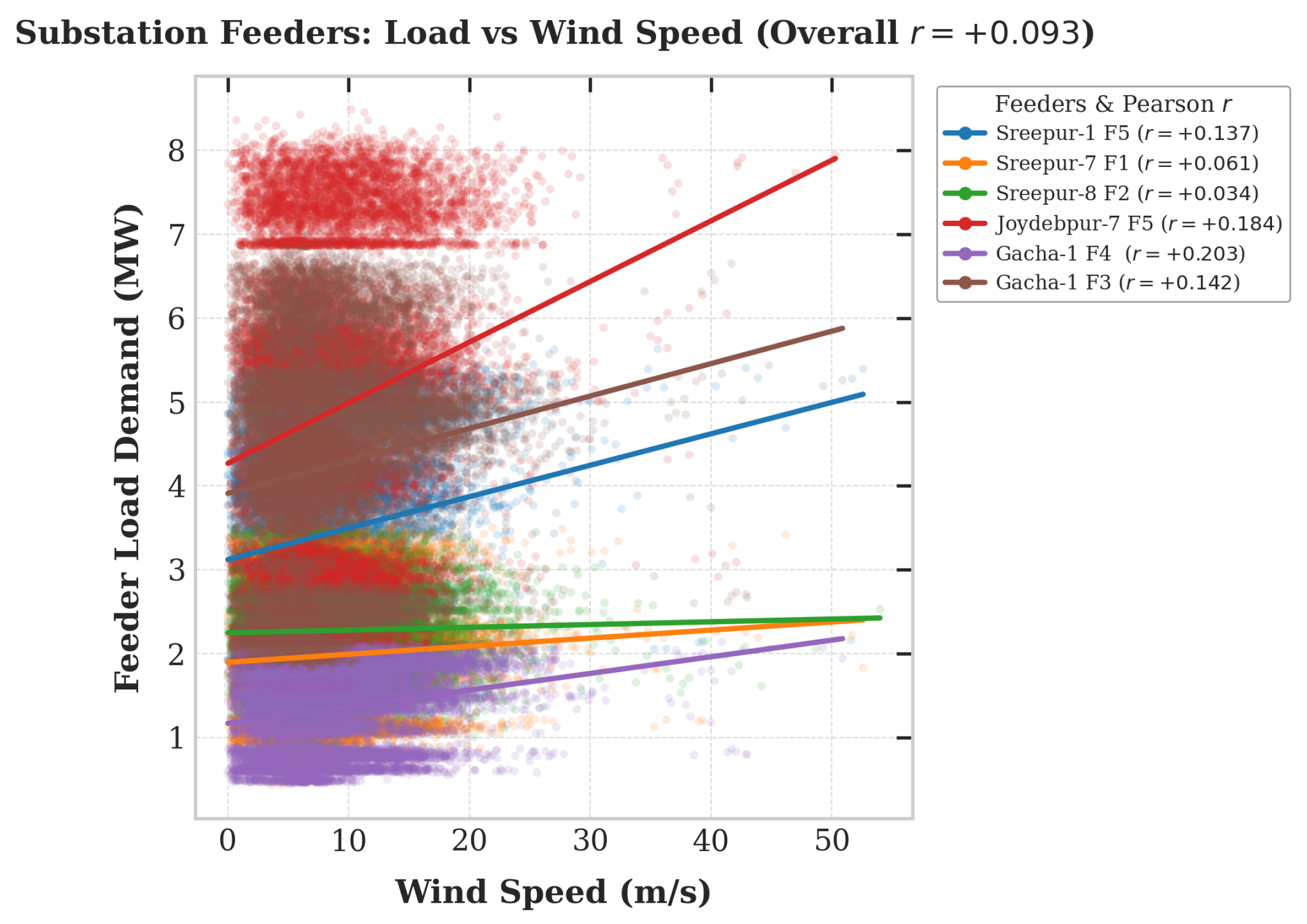
Conversely, local wind speed (Figure 7) shows a weak overall positive correlation ($r=+0.093$), ranging from $r=+0.203$ on Gacha-1 F4 to $r=+0.034$ on Sreepur-8 F2, driven by a diurnal increase in wind speed coinciding with afternoon industrial load ramps.

Figure 7. Multi-feeder correlation analysis between local wind speed and electrical demand, illustrating weak positive correlation trends ($r=+0.093$).

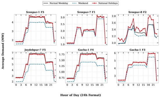
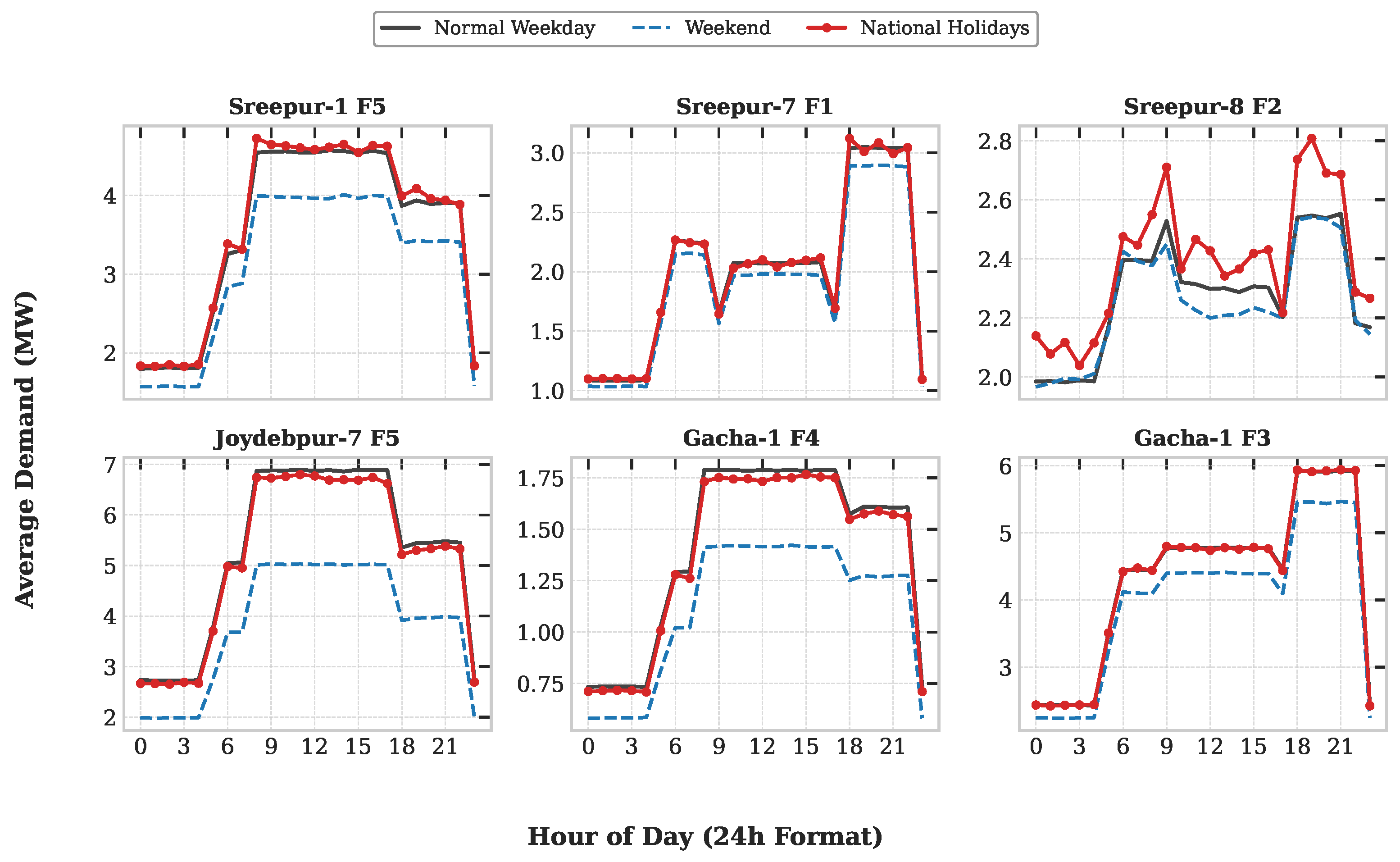
Electricity consumption shifts during non-working days and major cultural events, as illustrated in (Figure 8), validating the integration of binary indicator variables for weekends, daily operating windows, and holidays like Eid.

Figure 8. Comparative analysis of hourly demand profiles across six individual distribution feeders, illustrating distinct consumption patterns for normal weekdays, weekends, and national holidays.

4.3. 1-Step-Ahead Forecasting Performance

As summarized in Table 5 and Table 6, tree-based ensemble architectures consistently demonstrated superior predictive performance across all six feeders, with Random Forest achieving the lowest overall Mean MAPE of 2.35%, closely followed by XGBoost (2.52% Mean MAPE) and LightGBM (2.56% Mean MAPE).

Table 5. Feeder-wise error evaluation (MAE, RMSE) across 1-step-ahead forecasting models. Feeders are labeled as Substation Name + Feeder Code (e.g., “Sreepur-1 F5” = Feeder 5 at the Sreepur-1 substation). MAE: Mean Absolute Error (MW); RMSE: Root Mean Squared Error (MW).

Category	Model	Sreepur-1 F5		Sreepur-7 F1		Sreepur-8 F2		Joydebpur-7 F5		Gacha-1 F4		Gacha-1 F3
		MAE	RMSE	MAE	RMSE	MAE	RMSE	MAE	RMSE	MAE	RMSE	MAE	RMSE
		(MW)	(MW)	(MW)	(MW)	(MW)	(MW)	(MW)	(MW)	(MW)	(MW)	(MW)	(MW)
Stat. Baselines	ARIMA	0.83	1.0184	0.46	0.5721	0.20	0.24	1.36	1.6682	0.32	0.4011	0.85	1.1076
	SARIMA	0.30	0.4116	0.08	0.1313	0.06	0.1045	0.47	0.6672	0.11	0.1495	0.17	0.2448
Linear Reg.	Linear Reg.	0.22	0.3119	0.08	0.1283	0.09	0.1265	0.27	0.3781	0.07	0.0902	0.16	0.2187
Tree Ensembles	LightGBM	0.09	0.1263	0.06	0.1030	0.03	0.0505	0.11	0.1484	0.03	0.0466	0.10	0.1343
	XGBoost	0.08	0.1196	0.06	0.1031	0.03	0.0487	0.11	0.1477	0.03	0.0454	0.10	0.1344
	Random Forest	0.06	0.0922	0.06	0.1058	0.02	0.0460	0.10	0.1606	0.03	0.0463	0.09	0.1345
Deep Learning	LSTM	0.17	0.2282	0.07	0.1135	0.09	0.1241	0.26	0.3464	0.04	0.0524	0.13	0.1733
	GRU	0.14	0.2010	0.07	0.1110	0.05	0.0701	0.17	0.2332	0.04	0.0551	0.10	0.1381

Table 6. Feeder-wise evaluation: MAPE (Mean Absolute Percentage Error) and $R^2$ score (Coefficient of Determination) calculated on test data across 1-step-ahead forecasting models.

Category	Model	Sreepur-1 F5		Sreepur-7 F1		Sreepur-8 F2		Joydebpur-7 F5		Gacha-1 F4		Gacha-1 F3		Metrics
		MAPE	R2	MAPE	R2	MAPE	R2	MAPE	R2	MAPE	R2	MAPE	R2	Mean MAPE
		(%)		(%)		(%)		(%)		(%)		(%)		(%)
Stat. Baselines	ARIMA	34.84	0.2622	31.31	0.3034	8.33	0.4940	40.78	0.1016	35.52	0.2052	28.55	0.2315	29.89
	SARIMA	9.42	0.8795	4.50	0.9633	2.40	0.9089	11.24	0.8563	8.98	0.8896	4.23	0.9625	6.79
Linear Reg.	Linear Reg.	7.39	0.9308	4.70	0.9649	3.43	0.8667	6.75	0.9539	5.96	0.9598	4.23	0.9700	5.41
Tree Ensembles	LightGBM	3.11	0.9887	3.46	0.9774	1.14	0.9788	2.46	0.9929	2.84	0.9893	2.36	0.9887	2.56
	XGBoost	3.02	0.9898	3.44	0.9773	1.07	0.9803	2.44	0.9930	2.81	0.9898	2.36	0.9887	2.52
	Random Forest	2.30	0.9940	3.52	0.9762	0.83	0.9825	2.36	0.9917	2.74	0.9894	2.32	0.9887	2.35
Deep Learning	LSTM	5.88	0.9630	4.02	0.9725	3.54	0.8720	5.20	0.9613	3.18	0.9864	3.32	0.9812	4.19
	GRU	4.64	0.9713	3.86	0.9738	1.94	0.9592	4.21	0.9825	3.27	0.9850	2.64	0.9880	3.43

In terms of absolute errors (Table 5), Random Forest attained the minimum MAE across five out of six feeders, reaching a peak precision of 0.02 MW MAE (0.0460 MW RMSE) on Sreepur-8 F2 and 0.06 MW MAE (0.0922 MW RMSE) on Sreepur-1 F5. XGBoost and LightGBM exhibited closely competitive RMSE bounds, with XGBoost recording the lowest RMSE on Joydebpur-7 F5 (0.1477 MW) and Gacha-1 F4 (0.0454 MW), while LightGBM led on Sreepur-7 F1 (0.1030 MW) and Gacha-1 F3 (0.1343 MW).

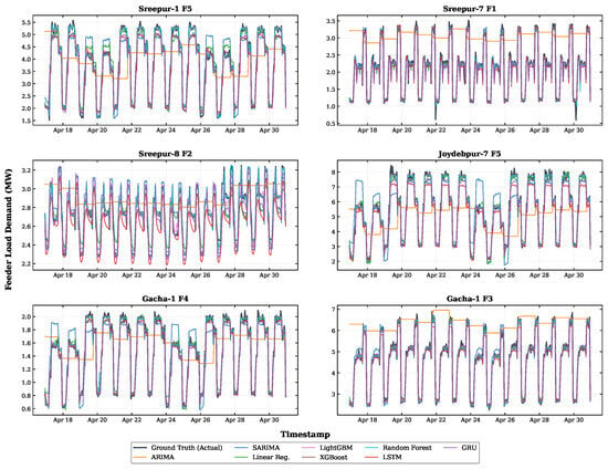
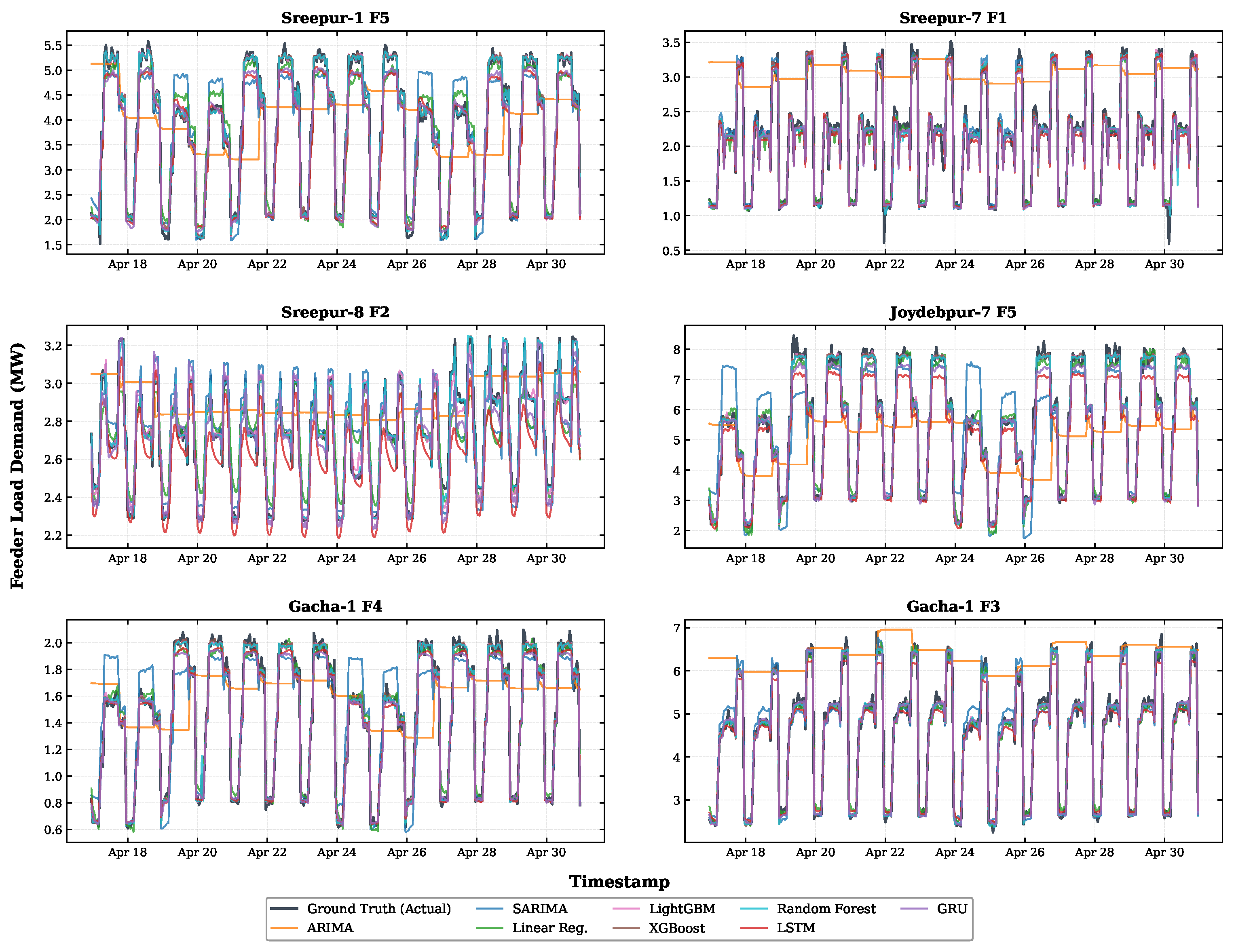
Goodness-of-fit evaluations on test data (Table 6) further reinforce the robustness of the ensemble models, all maintaining $R^2$ scores exceeding 0.976 across all feeders and reaching up to 0.9940 (Random Forest on Sreepur-1 F5). The deep learning architectures (GRU and LSTM) formed the next best performing class, achieving Mean MAPEs of 3.43% ($R^2\ge 0.9592$) and 4.19% ($R^2\ge 0.8720$), respectively, outperforming linear regression (5.41% Mean MAPE). The statistical baselines struggled on dynamic load profiles, with SARIMA achieving a 6.79% Mean MAPE, whereas standard ARIMA exhibited significant residual tracking errors, yielding negative test $R^2$ values on Sreepur-7 F1 (−1.4604) and Gacha-1 F3 (−1.3978) due to severe uncaptured non-stationarity. Visual inspection of the 14-day forecast horizon (Figure 9) confirms that tree ensembles closely track ground-truth load profiles across both peak industrial hours and non-working demand dips.

Figure 9. Comparative evaluation of 1-step-ahead hourly load forecasting models evaluated across a 14-day test window (336 consecutive hours) for six primary distribution feeders. Ground-truth actual load demand is highlighted in bold and slated against machine learning and statistical model predictions.

4.4. Multi-Step Rolling Horizon Forecasting and Statistical Validation

When evaluating long-term multi-step performance over the 168 h recursive rolling horizon across 24 evaluation windows in the full test set (Table 7 and Table 8), a clear operational divergence emerges. While deep learning sequence models (LSTM and GRU) performed competitively in static single-step tests, they exhibited severe autoregressive error propagation over the continuous $h=168$ forecast window, resulting in average MAPEs exceeding 17% (specifically reaching 17.29% for LSTM and 19.67% for GRU) and negative $R^2$ scores on volatile feeders, such as $-0.5123$ for LSTM on Sreepur-7 F1 and $-0.3122$ for GRU on Gacha-1 F3.

Table 7. Feeder-wise 168-hour rolling forecast performance matrix (MAE and RMSE) across machine learning models. Feeders are labeled as Substation Name + Feeder Code (e.g., “Sreepur-1 F5” = Feeder 5 at the Sreepur-1 substation). MAE: Mean Absolute Error (MW); RMSE: Root Mean Squared Error (MW).

Category	Model	Sreepur-1 F5		Sreepur-7 F1		Sreepur-8 F2		Joydebpur-7 F5		Gacha-1 F4		Gacha-1 F3		Overall Average
		MAE	RMSE	MAE	RMSE	MAE	RMSE	MAE	RMSE	MAE	RMSE	MAE	RMSE	Avg MAE	Avg RMSE
		(MW)	(MW)	(MW)	(MW)	(MW)	(MW)	(MW)	(MW)	(MW)	(MW)	(MW)	(MW)	(MW)	(MW)
Baseline Models	Persistence (Lag-168)	0.1634	0.2951	0.0948	0.1602	0.0627	0.1269	0.2026	0.3869	0.0584	0.0995	0.1625	0.2684	0.1241	0.2228
	Linear Regression	0.2259	0.3128	0.0830	0.1307	0.0875	0.1304	0.2823	0.3940	0.0701	0.0951	0.1699	0.2374	0.1531	0.2168
Tree Ensembles	LightGBM	0.1353	0.2367	0.0679	0.1201	0.0606	0.1171	0.1651	0.3395	0.0480	0.0872	0.1229	0.2100	0.1000	0.1851
	XGBoost	0.1453	0.2503	0.0677	0.1201	0.0551	0.1082	0.1644	0.3352	0.0455	0.0826	0.1195	0.2060	0.0996	0.1837
	Random Forest	0.1183	0.2229	0.0687	0.1220	0.0473	0.1116	0.1634	0.3444	0.0426	0.0795	0.1152	0.2024	0.0926	0.1805
Deep Learning	LSTM	0.4225	0.6037	0.5925	0.8417	0.2285	0.2978	0.7595	1.0347	0.1578	0.2407	0.5786	0.9763	0.4566	0.6658
	GRU	0.4401	0.6570	0.4707	0.5810	0.1494	0.2145	0.8725	1.0939	0.2233	0.3353	0.9966	1.4447	0.5254	0.7211

Table 8. Feeder-wise 168-hour rolling forecast performance matrix (MAPE and $R^2$) across machine learning models. Feeders are labeled as Substation Name + Feeder Code (e.g., “Sreepur-1 F5” = Feeder 5 at the Sreepur-1 substation). MAPE: Mean Absolute Percentage Error (%); $R^2$: Coefficient of Determination.

Category	Model	Sreepur-1 F5		Sreepur-7 F1		Sreepur-8 F2		Joydebpur-7 F5		Gacha-1 F4		Gacha-1 F3		Overall Average
		MAPE	R2	MAPE	R2	MAPE	R2	MAPE	R2	MAPE	R2	MAPE	R2	Avg MAPE	Avg R2
		(%)		(%)		(%)		(%)		(%)		(%)		(%)
Baseline Models	Persistence (Lag-168)	5.09	0.9376	5.12	0.9450	2.38	0.8635	4.30	0.9513	4.63	0.9507	3.94	0.9545	4.24	0.9338
	Linear Regression	7.51	0.9301	4.74	0.9635	3.51	0.8574	6.95	0.9497	6.20	0.9552	4.45	0.9646	5.56	0.9368
Tree Ensembles	LightGBM	4.51	0.9600	3.74	0.9692	2.30	0.8850	3.51	0.9627	3.77	0.9623	2.97	0.9723	3.47	0.9519
	XGBoost	4.81	0.9553	3.72	0.9692	2.12	0.9020	3.48	0.9636	3.60	0.9662	2.89	0.9733	3.44	0.9549
	Random Forest	3.90	0.9645	3.78	0.9682	1.80	0.8957	3.46	0.9616	3.38	0.9687	2.79	0.9742	3.19	0.9555
Deep Learning	LSTM	14.71	0.7399	33.38	-0.5123	8.85	0.2567	16.28	0.6533	14.81	0.7130	15.73	0.4007	17.29	0.3752
	GRU	14.53	0.6919	34.49	0.2794	5.99	0.6146	22.50	0.6125	18.06	0.4431	24.46	−0.3122	19.67	0.3882

Consequently, only the persistence baseline model and the tree-based ensemble models (LightGBM, Random Forest, and XGBoost) demonstrated robust, non-divergent forecasting trajectories across the entire 168 h rolling evaluation, with Random Forest recording the lowest overall average MAPE of 3.19% (and overall average MAE of 0.0926 MW and RMSE of 0.1805 MW, as detailed in Table 7 and Table 8), closely followed by XGBoost at 3.44% MAPE and LightGBM at 3.47% MAPE. For this reason, formal statistical significance testing—comprising pair-wise Diebold–Mariano (DM) tests and Wilcoxon signed-rank tests ($\alpha =0.05$)—was conducted exclusively among the tree ensembles and the naive persistence baseline (Table 9).

Table 9. Statistical significance tests across the test set (24 rolling windows with 168 h horizon, each model having 4032 data points).

Model Comparison	DM Stat (h = 168)	DM p-Value	Wilcoxon p-Value	Significant? (α = 0.05)
LightGBM vs. Persistence	14.8435	<0.0001	<0.0001	Yes (Model Superior)
RandomForest vs. Persistence	14.8644	<0.0001	<0.0001	Yes (Model Superior)
XGBoost vs. Persistence	14.8696	<0.0001	<0.0001	Yes (Model Superior)
LightGBM vs. RandomForest	0.7806	0.4350	<0.0001	No (Equivalent)
LightGBM vs. XGBoost	−0.0970	0.9227	0.0791	No (Equivalent)
RandomForest vs. XGBoost	−0.9317	0.3515	<0.0001	No (Equivalent)

The statistical tests confirmed that all three tree models significantly outperformed the persistence benchmark ($p<0.0001$). However, the pair-wise DM test revealed no statistically significant performance difference between the tree architectures themselves (LightGBM vs. Random Forest: $p=0.4350$; LightGBM vs. XGBoost: $p=0.9227$). Because LightGBM achieves statistically equivalent performance while drastically reducing 168 h horizon inference latency to just 0.55 s per window—compared to 1.37 s for XGBoost and 15.15 s for Random Forest—and maintaining a minimal model size of 1.2 MB (a 100-fold reduction from Random Forest’s 120 MB and smaller than XGBoost’s 1.5 MB), alongside a highly efficient training time of 3.47 s (Table 10), it avoids memory bandwidth bottlenecks and represents the optimal candidate for resource-constrained edge deployment in BREB distribution substations.

Table 10. Computational efficiency and deployment metrics across top 5 forecasting models. Inference time measured on 168 h rolling forecast.

Model	Training Time (s)	Model Size (MB)	Inference Time (s)
Tree Ensembles
LightGBM	3.47	1.2	0.55
XGBoost	7.92	1.5	1.37
Random Forest	235.30	120.0	15.15
Deep Learning Models
LSTM	321.86	0.42	18.07
GRU	385.95	0.53	15.48

4.5. Predictive Uncertainty and Risk Analysis

To quantify forecast risk across multi-step horizon rollouts, empirical prediction intervals were evaluated using non-overlapping 24 h evaluation windows extracted from the test set across all six distribution feeders. For each discrete horizon step $h\in \{1,2,\dots ,24\}$, the relative uncertainty margin $U_h$ ($\pm \%$) under a $95\%$ statistical confidence level ($\alpha =0.05$, $z_{0.025}=1.96$) is computed as

$$U_h=\left({\displaystyle \frac{1.96·{\sigma }_{e,h}}{{\overline{y}}_h}}\right)\times 100$$

(2)

where ${\sigma }_{e,h}$ represents the sample standard deviation ($\mathtt{ddof}=1$) of model forecast residuals $e_{i,h}=y_{i,h}-{\widehat{y}}_{i,h}$ across N test windows, and ${\overline{y}}_h$ denotes the mean observed feeder load at step h. Here, $U_h$ serves as a normalized parametric proxy for relative error dispersion across evaluation windows under asymptotic Gaussian assumptions.

The uncertainty analysis demonstrates that tree-based models, particularly LightGBM, achieve superior variance bounds compared to deep learning architectures—a finding that aligns with recent probabilistic forecasting where LGBM-Q performed better than DeepAR and MQRNN [26].

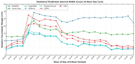
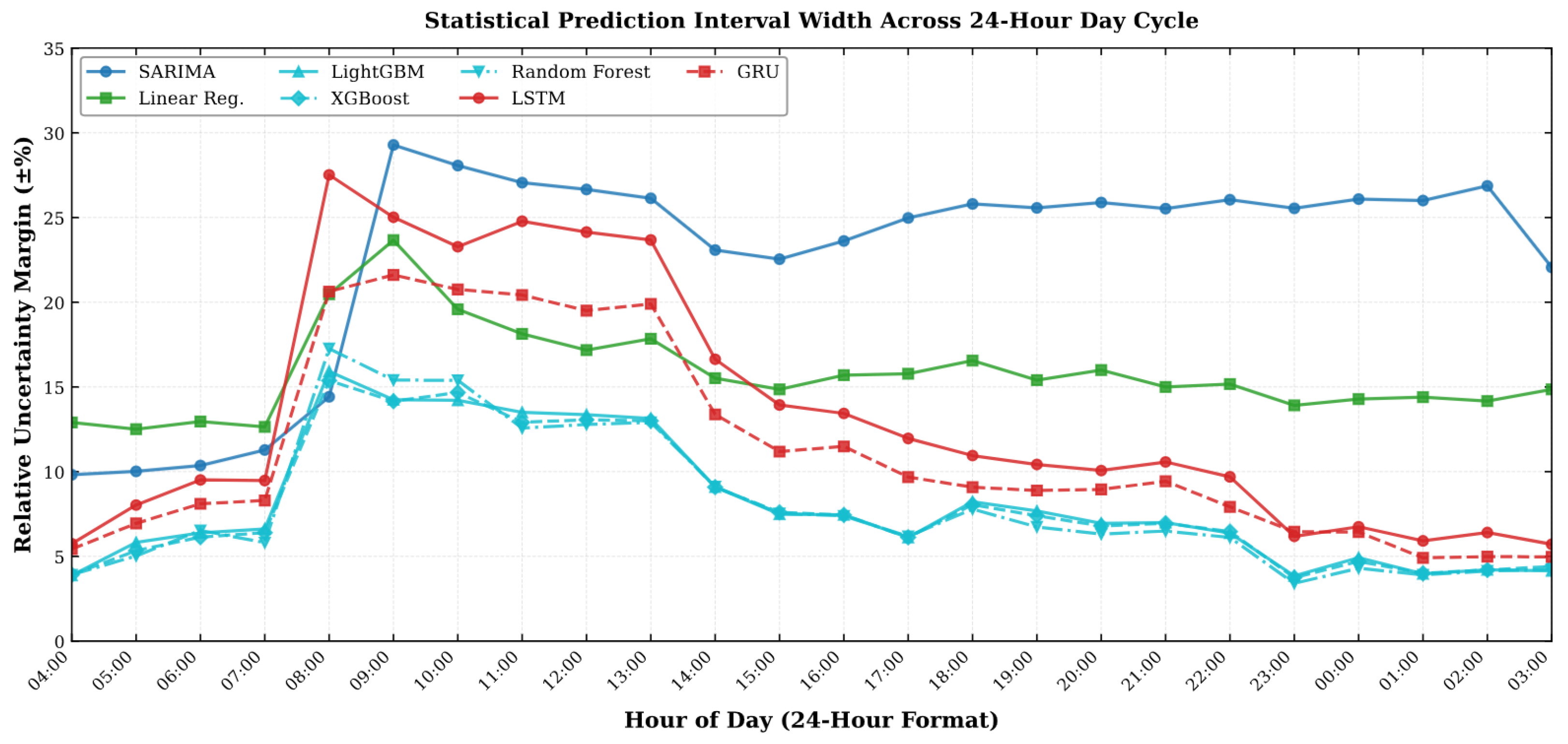
As illustrated in Figure 10, predictive uncertainty exhibits severe heteroscedasticity linked to diurnal grid dynamics over the 24 h look-ahead horizon starting at 04:00:

Figure 10. Statistical prediction interval margins (±%) across the 24 h look-ahead horizon starting at the test forecast origin (04:00). Computed at a $95\%$ confidence level ($1.96{\sigma }_e/\overline{y}$). Note: ARIMA is omitted due to relative uncertainty margins exceeding $100\%$.

• Early Morning Base (Step 1–4/04:00–07:00): Forecast risk remains tightly constrained during low-demand off-peak hours. Tree ensembles (LightGBM, XGBoost, Random Forest) deliver the narrowest uncertainty bands, ranging from $\pm 3.9\%$ to $\pm 6.8\%$. Linear regression establishes a near-constant baseline around $\pm 12.5$–$\pm 12.8\%$.
• Diurnal Ramp-Up Surge (Step 5–6/08:00–09:00): Rapid industrial shift initiations and load ramping trigger a sharp expansion in residual variance. LSTM and GRU experience an immediate spike at Step 5 (08:00), expanding to relative uncertainty margins of $\pm 27.4\%$ and $\pm 20.6\%$, respectively. SARIMA reaches its overall maximum uncertainty of $\pm 29.1\%$ at Step 6 (09:00). Tree ensembles display strong robustness during this transition, bounding uncertainty to $\pm 15.8$–$\pm 17.2\%$.
• Midday Industrial Operating Plateau (Step 7–10/10:00–13:00): LSTM retains an elevated risk profile fluctuating between $\pm 23.2$ and $\pm 24.7\%$, whereas tree-based ensembles rapidly cool down to a stable $\pm 12.6$–$\pm 15.8\%$ interval.
• Overnight Convergence (Step 20–24/23:00–03:00): As grid operational variance drops overnight, all machine learning architectures converge toward minimal uncertainty. Tree ensembles hit their global minimum at Step 20 (23:00), shrinking to $\pm 3.4$–$\pm 4.0\%$. GRU and LSTM decay to $\pm 5.1\%$ and $\pm 5.7\%$ by Step 24 (03:00), while non-seasonal ARIMA is excluded from the analysis as its relative uncertainty exceeds $100\%$.

5. Discussion

The benchmarking results highlight a clear trade-off between predictive accuracy and computational footprint across model families. While non-linear tree-based ensembles consistently dominated the top performance tier, their operational deployment characteristics vary significantly:

• MAE/MAPE Precision vs. Memory Footprint: Random Forest achieved the lowest overall average error ($2.35\%$ Mean MAPE; $0.06\mathrm{MW}$ MAE on Sreepur-1 F5) and the lowest single-feeder MAPE ($0.83\%$ with $0.02\mathrm{MW}$ MAE on Sreepur-8 F2). However, this marginal gain over gradient boosting frameworks comes at the cost of a massive model file size ($120\mathrm{MB}$) and a high inference latency of 15.15 s, as shown in Table 10.
• Optimal Production Selection: LightGBM established the most favorable operational profile, achieving a highly competitive $2.56\%$ Mean MAPE while executing in just $0.55\mathrm{s}$ with a lightweight $1.2\mathrm{MB}$ footprint, making it the ideal candidate for real-time edge integration in automated feeder load management. These findings align directly with recent empirical benchmarks on real-world power distribution systems, such as those of Shiblee and Koukaras (2025) [17], who similarly demonstrated that LightGBM systematically outperforms deep recurrent architectures (LSTM, GRU) and hybrid CNN-LSTM networks across standard error metrics while maintaining superior computational efficiency and model interpretability.
• Deep Learning vs. Linear Baselines: Deep recurrent architectures captured diurnal dependencies effectively (GRU achieving a $3.43\%$ Mean MAPE and LSTM a $4.19\%$ Mean MAPE), but were outperformed by tree ensembles due to the strong tabular signal provided by the engineered 43-variable feature vector. Classical non-seasonal ARIMA failed to generalize ($29.89\%$ Mean MAPE) due to its inability to account for sudden holiday shocks and rapid industrial ramping.

Study Limitations and Operational Vulnerabilities

Despite the strong empirical performance of gradient-boosted tree ensembles, several operational boundaries and methodological limitations must be acknowledged:

• Susceptibility to Missing Lag Values: The 168 h recursive forecasting protocol is highly susceptible to missing or corrupted historical load lags, as an unhandled missing value at step t rapidly propagates through autoregressive feature updates across the remaining forecast horizon.
• Dependency on Meteorological Forecasting Quality: Predictive performance remains tightly coupled to the accuracy of external meteorological inputs, leaving the pipeline vulnerable to forecast errors or unexpected localized micro-climate shifts in the weather data stream.
• Geographic and Topological Boundaries:The empirical evaluation is restricted to six distribution feeders across two operational zones, limiting immediate zero-shot generalization to unobserved feeder topologies and densely populated urban networks without prior retraining.

6. Conclusions

This study addresses the critical challenge of localized short-term load forecasting at the feeder level, directly targeting the operational constraints of resource-constrained distribution substations under the Bangladesh Rural Electrification Board (BREB). While traditional national-scale models smooth out localized demand fluctuations, our multi-feeder benchmarking across Gazipur PBS-1 and Mymensingh PBS-2 demonstrates that capturing micro-climate variations and feeder-specific consumer behaviors requires a carefully balanced combination of domain-specific feature engineering and lightweight model architectures.

Addressing the core objective of balancing predictive precision against operational overhead, Random Forest achieved the minimum overall error (2.35% Mean MAPE, reaching 0.83% MAPE and 0.02 MW MAE on Sreepur-8 F2), but incurred substantial inference time for 168 h forecast (15.15 s) and memory footprint ($120\mathrm{MB}$), as shown in Table 10. In contrast, LightGBM achieved statistically equivalent accuracy (2.56% Mean MAPE; $p=0.4350$ in Diebold–Mariano testing) with a 168 h inference time of just 0.55 s and a minimal 1.2 MB footprint. This demonstrates that gradient-boosted tree ensembles offer the optimal balance of accuracy, scalability, and computational efficiency required for seamless deployment in real-time power quality monitoring dashboards and automated feeder dispatching across rural utility zones.

References

- Habbak, H.; Mahmoud, M.; Metwally, K.; Fouda, M.M.; Ibrahem, M.I. Load Forecasting Techniques and Their Applications in Smart Grids. Energies 2023, 16, 1480. [Google Scholar] [CrossRef] [Scilit]
- Hasan, M.; Mifta, Z.; Papiya, S.J.; Roy, P.; Dey, P.; Salsabil, N.A.; Chowdhury, N.U.R.; Farrok, O. A state-of-the-art comparative review of load forecasting methods: Characteristics, perspectives, and applications. Energy Convers. Manag. X 2025, 26, 100922. [Google Scholar] [CrossRef] [Scilit]
- Gasparin, A.; Lukovic, S.; Alippi, C. Deep learning for time series forecasting: The electric load case. CAAI Trans. Intell. Technol. 2022, 7, 1–25. [Google Scholar] [CrossRef] [Scilit]
- Islam, S.; Zaber, M.; Ali, A.A. A smart grid prerequisite: Survey on electricity demand forecasting models and scope analysis of demand forecasting in Bangladesh. In Proceedings of the 2017 IEEE Region 10 Humanitarian Technology Conference (R10-HTC), Dhaka, Bangladesh, 21–23 December 2017; pp. 691–696. [Google Scholar] [CrossRef] [Scilit]
- Rafi, S.H.; Nahid-Al-Masood; Deeba, S.R.; Hossain, E. A Short-Term Load Forecasting Method Using Integrated CNN and LSTM Network. IEEE Access 2021, 9, 32436–32448. [Google Scholar] [CrossRef] [Scilit]
- Hasan-Al-Shaikh; Rahman, M.A.; Zubair, A. Electric Load Forecasting with Hourly Precision Using Long Short-Term Memory Networks. In Proceedings of the 2019 International Conference on Electrical, Computer and Communication Engineering (ECCE), Cox’s Bazar, Bangladesh, 7–9 February 2019; pp. 1–6. [Google Scholar] [CrossRef] [Scilit]
- Nti, I.K.; Teimeh, M.; Nyarko-Boateng, O.; Adekoya, A.F. Electricity load forecasting: A systematic review. J. Electr. Syst. Inf. Technol. 2020, 7, 13. [Google Scholar] [CrossRef] [Scilit]
- Ullah, K.; Ahsan, M.; Hasanat, S.M.; Haris, M.; Yousaf, H.; Raza, S.F.; Tandon, R.; Abid, S.; Ullah, Z. Short-Term Load Forecasting: A Comprehensive Review and Simulation Study with CNN-LSTM Hybrids Approach. IEEE Access 2024, 12, 111858–111881. [Google Scholar] [CrossRef] [Scilit]
- Cordeiro-Costas, M.; Villanueva, D.; Eguía-Oller, P.; Martínez-Comesaña, M.; Ramos, S. Load Forecasting with Machine Learning and Deep Learning Methods. Appl. Sci. 2023, 13, 7933. [Google Scholar] [CrossRef] [Scilit]
- Zippenfenig, P. Open-Meteo.com Weather API, Version 0.2.69; Zenodo: Geneva, Switzerland, 2023. [CrossRef]
- Breiman, L. Random forests. Mach. Learn. 2001, 45, 5–32. [Google Scholar] [CrossRef] [Scilit]
- Chen, T.; Guestrin, C. XGBoost: A scalable tree boosting system. In Proceedings of the 22nd ACM SIGKDD International Conference on Knowledge Discovery and Data Mining, San Francisco, CA, USA, 13–17 August 2016; pp. 785–794. [Google Scholar] [CrossRef] [Scilit]
- Ke, G.; Meng, Q.; Finley, T.; Wang, T.; Chen, W.; Ma, W.; Ye, Q.; Liu, T.Y. LightGBM: A Highly Efficient Gradient Boosting Decision Tree. In Advances in Neural Information Processing Systems (NeurIPS 2017); Guyon, I., Luxburg, U.V., Bengio, S., Wallach, H., Fergus, R., Vishwanathan, S., Garnett, R., Eds.; Curran Associates, Inc.: Long Beach, CA, USA, 2017; Volume 30. [Google Scholar]
- Hochreiter, S.; Schmidhuber, J. Long short-term memory. Neural Comput. 1997, 9, 1735–1780. [Google Scholar] [CrossRef] [Scilit] [PubMed]
- Cho, K.; Van Merriënboer, B.; Gulcehre, C.; Bahdanau, D.; Bougares, F.; Schwenk, H.; Bengio, Y. Learning phrase representations using RNN encoder–decoder for statistical machine translation. arXiv 2014, arXiv:1406.1078. [Google Scholar]
- Magalhães, B.; Bento, P.; Pombo, J.; Calado, M.R.; Mariano, S. Short-Term Load Forecasting Based on Optimized Random Forest and Optimal Feature Selection. Energies 2024, 17, 1926. [Google Scholar] [CrossRef] [Scilit]
- Shiblee, M.F.H.; Koukaras, P. Short-Term Load Forecasting in the Greek Power Distribution System: A Comparative Study of Gradient Boosting and Deep Learning Models. Energies 2025, 18, 5060. [Google Scholar] [CrossRef] [Scilit]
- Kong, W.; Dong, Z.Y.; Jia, Y.; Hill, D.J.; Xu, Y.; Zhang, Y. Short-Term Residential Load Forecasting Based on LSTM Recurrent Neural Network. IEEE Trans. Smart Grid 2017, 8, 2811–2821. [Google Scholar] [CrossRef] [Scilit]
- Pavlatos, C.; Makris, E.; Fotis, G.; Vita, V.; Mladenov, V. Enhancing electrical load prediction using a bidirectional LSTM neural network. Electronics 2023, 12, 4652. [Google Scholar] [CrossRef] [Scilit]
- Abumohsen, M.; Owda, A.Y.; Owda, M. Electrical Load Forecasting Using LSTM, GRU, and RNN Algorithms. Energies 2023, 16, 2283. [Google Scholar] [CrossRef] [Scilit]
- Pentsos, V.; Tragoudas, S.; Wibbenmeyer, J.; Khdeer, N. A Hybrid LSTM-Transformer Model for Power Load Forecasting. IEEE Trans. Smart Grid 2025, 16, 2624–2634. [Google Scholar] [CrossRef] [Scilit]
- Figueiró, I.C.; Abaide, A.R.; Knak Neto, N.; Silva, L.N.F.; Santos, L.L.C. Bottom-Up Short-Term Load Forecasting Considering Macro-Region and Weighting by Meteorological Region. Energies 2023, 16, 6857. [Google Scholar] [CrossRef] [Scilit]
- Liu, H.; Wang, Y.; Wei, C.; Li, J.; Lin, Y. Two-Stage Short-Term Load Forecasting for Power Transformers Under Different Substation Operating Conditions. IEEE Access 2019, 7, 161424–161436. [Google Scholar] [CrossRef] [Scilit]
- Akarne, Y.; Essadki, A.; Nasser, T.; Annoukoubi, M. Enhanced smart microgrid scheduling: An empirical study on simultaneous energy supply and demand optimization using binary sparrow search algorithm. Results Eng. 2025, 27, 106811. [Google Scholar] [CrossRef] [Scilit]
- Shahinzadeh, H.; Nafisi, H.; Zamani, A.; Mehrabani-Najafabadi, S.; Mahmoudi, A.; Ebrahimi, F. Probabilistic Short-Term Load Forecasting Using GBDT-Based Sister Forecasts and Ensemble Methods. In Proceedings of the 2025 15th International Conference on Computer and Knowledge Engineering (ICCKE), Mashhad, Iran, 28–29 October 2025. [Google Scholar]
- Ryu, S.; Yu, J.B. Quantile-Mixer: A Novel Deep Learning Approach for Probabilistic Short-Term Load Forecasting. IEEE Trans. Smart Grid 2024, 15, 2237–2250. [Google Scholar] [CrossRef] [Scilit]
Disclaimer/Publisher’s Note: The statements, opinions and data contained in all publications are solely those of the individual author(s) and contributor(s) and not of MDPI and/or the editor(s). MDPI and/or the editor(s) disclaim responsibility for any injury to people or property resulting from any ideas, methods, instructions or products referred to in the content. |
© 2026 by the authors. Licensee MDPI, Basel, Switzerland. This article is an open access article distributed under the terms and conditions of the Creative Commons Attribution (CC BY) license.