


Abstract
Electricity market settlement rules shape the financial exposure of energy aggregators when generation deviates from contracted positions, yet their interaction with Conditional-Value-at-Risk (CVaR) based risk aversion in aggregator scheduling remains unexplored. This paper studies how imbalance penalty design shapes the risk–return tradeoff in a stochastic unit commitment framework for a network-constrained aggregator with a diversified generation portfolio. Five settlement regimes are compared, spanning liberal, baseline, and strict penalty levels together with two zero-contract regimes that settle all exchange as imbalance. The risk-aversion weight is swept at a fixed confidence level on a modified IEEE 9-bus system using 200 stochastic scenarios, complemented by a continuous penalty-multiplier sweep. Stricter settlement disproportionately increases tail-risk exposure at the risk-neutral baseline, with the excess tail-risk ratio rising from 49% under liberal to 89% under strict penalties. Risk weighting reduces CVaR by 1.5–7.1% for an expected-profit sacrifice of at most 1.2%, with the largest absolute reductions where baseline tail risk is highest. Battery storage throughput falls by 22–35 MWh/day under market-participatory regimes but changes by less than 5 MWh/day once the contracted position is removed, becoming effectively invariant to the risk weight. The results give quantitative guidance on how settlement regime should inform aggregator risk management.
1. Introduction
The rapid growth of variable renewable energy sources (RES) and battery energy storage systems (BESS) has transformed energy aggregators into key market participants that must jointly coordinate diversified portfolios, optimize market positions, and manage the financial consequences of forecast uncertainty [1,2]. In liberalized electricity markets, aggregators submit day-ahead (DA) contracts and are subsequently exposed to imbalance settlement: any deviation between realized generation or consumption and the contracted position is financially settled by the transmission system operator (TSO) at prevailing penalty rates. The design of these settlement rules varies significantly across European markets, ranging from mild dual-price mechanisms to strict fixed-penalty regimes and self-balancing requirements [3,4].
Stochastic unit commitment (SUC) has emerged as the standard framework for scheduling aggregator portfolios under renewable uncertainty. Risk-neutral SUC minimizes expected operating cost across scenarios but can leave the aggregator exposed to large losses in rare but severe outcomes. Conditional Value-at-Risk (CVaR) has therefore been incorporated into the objective function to provide explicit control over tail-risk exposure, through a risk-aversion weight that linearly combines expected cost with the average cost in the worst (1-) fraction of scenarios [5,6].
Despite substantial work on risk-averse scheduling for individual resources and system operators [7,8], the interaction between settlement design and the suitable risk weight for aggregator portfolios has received little attention. The only closely related study is [9], which shows that one-price versus two-price imbalance settlement significantly changes the risk-aversion level needed to optimize an energy storage operator’s day-ahead bid. However, that analysis is limited to a single storage asset without a full generation portfolio or network constraints.
Using a risk-based stochastic UC framework developed for this study, this paper provides a systematic analysis of how market settlement design shapes the risk-return tradeoff for a network-constrained aggregator with a diversified portfolio. Five settlement regimes are evaluated over a continuous sweep, producing the following contributions:
- A comparative analysis of expected profit and risk across five settlement regimes at the risk-neutral baseline, quantifying the baseline tail-risk induced purely by penalty structure.
- A parametric characterization of how affects expected profit, CVaR, BESS throughput, and imbalance penalty exposure across regimes, revealing regime-dependent saturation behavior.
- Evidence that BESS responsiveness to CVaR weighting is suppressed under self-balancing rules: daily storage throughput becomes nearly invariant to , while the risk weight continues to reshape the intra-day timing of dispatch.
- A continuous penalty-multiplier sweep that resolves the discrete settlement regimes as points on a single curve and disentangles the effect of settlement stringency from that of the risk-aversion weight.
This framework was introduced in a companion study [10], which analyzes the CVaR confidence level and risk-aversion weight for a single market setup; the present paper reuses that framework as a validated vehicle and contributes a distinct analysis of how imbalance settlement design shapes the risk–return tradeoff, a dimension not considered in [10].
The rest of the paper is organized as follows. Section 1 covers the literature review. Section 2 briefly describes the optimization model, how the settlement regimes are defined and how the analysis is organized. Section 3 presents the case study. Section 4 presents and elaborates on the results. Section 5 discusses findings, limitations and future work. Section 6 concludes the paper.
Literature Review
Two-stage stochastic UC has become the standard tool for scheduling under RES uncertainty. First-stage commitment decisions are fixed day-ahead while second-stage dispatch adapts to each renewable and demand scenario. Risk-neutral SUC formulations minimize expected cost or maximize expected profit [11], but this leaves the aggregator exposed to extreme outcomes in the tail of the cost distribution.
Recent studies continue to extend this framework: a two-stage stochastic UC model has been developed for large-scale planning under combined renewable and electric-vehicle variability [12], and day-ahead dispatch optimization has been applied to insular systems with hydro-pumped storage and high renewable penetration [13].
A foundational benchmark for risk-based risk-averse scheduling under renewable uncertainty is established in [14], which demonstrates that risk assessment substantially reduces tail-risk exposure relative to risk-neutral stochastic unit commitment in isolated systems.
CVaR has been widely adopted to address this shortcoming because it is a coherent risk measure that can be embedded in a mixed-integer linear program (MILP) [5]. In [6] the value of multi-stage over two-stage stochastic programming is evaluated for risk-averse unit commitment models, showing that scheduling flexibility increases with the level of uncertainty and decreases with the degree of risk aversion, which provides context for the two-stage CVaR-based approach adopted in this study. In [7] stochastic scheduling for hydro-dominated systems with weekly energy storage is developed using a hybrid decomposition approach. The paper demonstrates that risk-aware solutions reduce exposure to adverse inflow scenarios at the cost of higher expected operating expenditure.
A network-constrained perspective on CVaR-based scheduling with battery storage is provided in [15], where storage participation is shown to alleviate ramping burdens and constrain real-time imbalance risk in a contingency-constrained unit commitment setting, though without considering the effect of settlement design itself.
Aggregators coordinate heterogeneous distributed energy resources (DER) and act as single market participants on behalf of local producers and consumers [1]. Security-constrained UC and economic dispatch (ED) remain the dominant operational frameworks for joint commitment, dispatch, and market participation optimization [11]. In [16] a risk-averse scheduling framework is applied to interconnected microgrids with price-responsive demand, showing that risk-averse hedging significantly reduces tail-cost exposure under price uncertainty. However, the role of penalty structure in shaping the appropriate level of risk aversion is not examined. Risk-constrained energy management has likewise been applied to multi-energy multi-microgrid systems with integrated demand response using hybrid risk-assessment approaches [17].
Closely related to the present market-oriented setting, a pan-European CVaR-constrained stochastic UC has been formulated jointly across day-ahead and intraday markets [18], while a mixed CVaR/information-gap framework has been applied to a multi-energy system participating in multiple energy markets [19]. These works confirm the suitability of CVaR for market-facing scheduling but do not examine how the imbalance settlement structure itself reshapes the suitable risk weight.
Recent work has extended risk-averse aggregator scheduling beyond a single asset class: [20] develops a risk-based coordinated trading strategy for load aggregators with energy storage across both spot and demand-response markets, while [21] evaluates the impact of risk measures and degradation cost specifically on battery storage arbitrage schedules. Risk-averse bidding for virtual power plants, a closely related aggregator archetype, has also been comprehensively surveyed in [22], which categorizes risk-based and robust optimization approaches across resource types. Complementary risk-based bidding frameworks have additionally been proposed for other distributed aggregator classes, including electric vehicle aggregators [23] and frequency-regulation virtual power plants [24], underscoring the breadth of recent interest in risk-averse aggregator participation.
Imbalance settlement rules define how deviations from contracted energy positions are financially reconciled. Mechanisms range from single-price systems, where one price applies to both positive and negative imbalances, to dual price systems with asymmetric shortfall and over-delivery penalties, to self-balancing requirements that prohibit contracted exchange entirely [3,4]. Paper [4] proposes a separated dual-price penalty mechanism as an incentive for self-balancing and shows analytically that stricter penalties reduce deviation volumes across market parties. Paper [3] demonstrates that a rolling horizon management approach reduces real-time imbalances for a renewable energy community operating under self-balancing rules, but does not examine the interaction with risk-aversion parameters.
The financial consequences of imbalance settlement design for aggregators have also been examined empirically: [25] develops a simulation model quantifying the balancing costs borne by renewable energy aggregators under the Greek market’s non-compliance charge structure, while [26] examines how renewable energy aggregators in Nordic markets can limit their imbalance settlement costs by choosing between internal balancing and balancing market participation, showing that the optimal strategy depends on forecast accuracy and the prevailing penalty structure.
The closest antecedent to this study is [9], which compares one-price and two-price imbalance settlement for a risk-averse energy storage operator in the Swedish market. That analysis finds that the two-price system, which imposes a fixed deviation fee, results in more moderate day-ahead bids and requires a CVaR weight to achieve optimal risk management compared to the one-price system . Although this directly motivates the present research question, the model in [9] covers only a single asset without a generation portfolio, network constraints, or the self-balancing regime.
No published study has systematically evaluated how the imbalance penalty structure affects the CVaR risk-return tradeoff across the full parametric range of for a network-constrained aggregator with a diversified portfolio. In particular, the behavior of BESS utilization and penalty exposure as a function of under qualitatively different settlement designs, including the removal of the contracted position (a settlement-induced self-balancing incentive), has not been characterized. This paper addresses that gap.
Table 1 gives a comparison of relevant literature to the work in this paper.
Table 1.
Positioning relative to representative literature. Agg.: aggregator-centric profit perspective; Net.: network-constrained model; Settle.: compares distinct imbalance settlement designs; -sweep: parametric sweep of the risk-aversion weight; Self-bal.: includes a zero-contract/self-balancing regime.
2. Methodology
For the goals of the study the authors used an aggregator-oriented stochastic scheduling model that solves an hourly UC/ED problem under renewable uncertainty, based on a MILP formulation [10]. The model takes the perspective of a single energy aggregator that coordinates a diversified portfolio on behalf of its local producers and consumers and participates in the wholesale day-ahead market on their behalf. Accordingly, the objective minimizes the aggregator’s own net operating cost (generation, storage degradation, imbalance and carbon penalties, net of revenue from supplying local demand and from market exchange) rather than a system-wide or social cost. The model supports different types of dispatchable units, RES (hydro power plants (HPP), solar photovoltaic (PV) and wind power plants (WPP)), BESS, and single or multiple PCCs for exchange with the central grid. A 24 h optimization is performed in the study.
The optimization is performed following day-ahead market clearing: the contracted quantity and the hourly day-ahead price for each hour are therefore known inputs, and the aggregator schedules its portfolio against them. Any failure to meet demand, or mismatch against the contracted position, is settled as an imbalance and priced through the shortfall and over-delivery penalties described below. Additionally, carbon-dioxide-related penalties are explicitly incorporated into the objective function of the model.
Inputs of the model include: generator data, PV and WPP generation, power demand data, BESS data, network line data and market data.
Because the developed model isn’t the focus of this paper, the full mathematical formulation will not be explained in detail. The risk-adjusted objective of the model is:
where is the total net cost in scenario s (generation, BESS degradation, penalties, minus revenues), is the equal scenario probability, is the VaR proxy, is the excess cost above , and is the risk-aversion weight. Setting recovers the risk-neutral stochastic UC.
The full model comprises 50 variable types and 77 constraint categories; a more detailed derivation is given in [10]. The constraints that bear directly on the settlement-regime analysis are reproduced below, while the remainder (generator minimum up/down times, reserve requirements, and the detailed piecewise cost linearization) follow [10].
For every hour, dispatchable generation, net storage discharge, renewable dispatch and unserved energy must equal net demand:
where , , and are the sets of dispatchable generators, BESS units, wind and PV plants; , and are the corresponding dispatch quantities; and are storage charge and discharge power; and is energy not served (ENS) in scenario s at hour t. Grid exchange at the point of common coupling (PCC) is modeled as a dispatchable resource whose signed power () is positive on import and negative on export, so no separate exchange variable is required.
The net PCC exchange is settled against the contracted day-ahead position, and its signed departure is split into a shortfall and an over-delivery component:
where is the contracted day-ahead quantity at hour t, is the shortfall (net exchange below contract) and the over-delivery (net exchange above contract). These are the variables penalized in the settlement terms of the cost function (9); under the zero-contract regimes S4 and S5, and the entire PCC exchange is therefore registered as deviation. Following the sign convention introduced above, PCC power () is positive on import and negative on export; consistently, a day-ahead export position has . The contracted quantities in Table A3 are reported as export magnitudes .
Dispatchable units operate between their power bounds only when committed, and renewable dispatch is capped by the scenario-dependent available output:
where , are the output limits of unit i, and is the first-stage commitment status of unit i at hour t, shared across all scenarios. When the unit is offline and its output is forced to zero; when the unit operates within . The quantities , are the available PV and wind outputs reflecting the sampled irradiance and wind-speed realizations.
Battery state of charge propagates according to
bounded by and a mutual-exclusion condition that prevents simultaneous charging and discharging, with , the charge and discharge efficiencies and , the binary status indicators.
Network security is imposed through a Generalized Generation Distribution Factor (GGDF) representation, so that the flow on each line l stays within its thermal rating:
where is the capacity of line l, the net injection at bus n, and the set of buses. Bus voltage magnitudes are held within their admissible band through a linearized Voltage Transfer Distribution Factor (VTDF) mapping with penalized slack variables, as detailed in [10].
The conditional value-at-risk in objective (1) is enforced through its standard epigraph reformulation:
where approximates the value-at-risk at confidence level and measures the cost excess of scenario s beyond ; together with the second term of (1) these yield the CVaR of the cost distribution.
The resulting objective function for a single scenario can be written as:
In (9), denotes the startup cost. represents the generation production cost of each unit per hour. The penalty on unserved energy is included to preserve the balance between generation and demand. BESS degradation for each unit is represented through the term , where is the marginal cost. The cost would be derived from the projected BESS operating life and cost during its operation. Market deviation variables and split the net deviation into shortfall and over-delivery of electrical energy, enabling settlement through penalties for shortfall and for over-delivery. In addition to penalties, deviations are also settled at the day-ahead price, corresponding to extra purchases to cover shortfall and reduced revenue (or buy-back) in case of over-delivery. Carbon costs are implemented through the CO2 price and unit emission factors . These are only for units that emit CO2.
The aggregator’s economic performance is evaluated as net profit, defined as total revenue minus total cost. Total cost comprises generation cost, BESS degradation, imbalance penalties, the day-ahead settlement of contracted and deviation quantities, and carbon cost. Total revenue comprises retail sales to served demand and the market value of net export (including export in excess of the contracted position). Net profit is their difference, evaluated per scenario and reported as the probability-weighted expectation across the scenario set.
The key methodological contribution of this paper is the definition of five settlement regimes applied to the same model and test system. The regimes differ only in penalty prices and contracted day-ahead quantity; all other inputs (generator data, network parameters, scenario sets, market prices) are held constant. The five regimes are defined as follows and summarized in Table 2.
Table 2.
Settlement regime definitions.
- S1—Liberal: Penalty prices are scaled to and , representing a market environment with mild imbalance costs. The contracted day-ahead quantity is the same as the baseline case.
- S2—Baseline: Historical values of hourly penalty prices and are used unmodified. The hourly contracted day-ahead quantity is predetermined and used as an input in the model.
- S3—Strict: Penalty prices are scaled to and , representing an environment with strong financial incentives to minimize deviations.
- S4—Self-balancing: The S3 penalty profile is retained, and the contracted day-ahead quantity is set to zero for all hours (). Grid exchange is not physically prohibited; rather, with no contracted position, every unit of import or export is registered as an imbalance deviation and settled at the S3 penalty rates.
- S5—Zero-contract, baseline penalty: The baseline (S2) penalty prices are retained while the contracted day-ahead quantity is set to zero (). This regime differs from S4 only in penalty level and from S2 only in the contracted position, so the pair of comparisons S4–S5 and S2–S5 isolates, respectively, the effect of penalty stringency and the effect of market participation on the risk–return outcome.
Formally, the five regimes are realized entirely through the settlement parameters of the cost function (9): S1–S3 scale the penalty prices and , S4 retains the S3 penalties and additionally sets ; and S5 sets at the baseline penalty level. No additional constraint restricts the power exchanged at the PCC in any regime; the market rule is imposed purely through the settlement terms, so the deviation variables and absorb the entire exchange under S4 and S5.
The zero-contract regimes (S4, S5) correspond to an aggregator that holds no day-ahead position and balances its portfolio in real time (for example a self-consuming energy community, microgrid, or prosumer aggregator under net-billing, or a balance-responsible party under a self-balancing obligation that settles all exchange at imbalance prices), with S4 and S5 representing a strict and a lenient imbalance-pricing regime, respectively.
The risk-aversion weight is swept over the range [0, 2.0]. For S1 a fine grid with step 0.1 (21 points) is used to resolve the saturation behavior in detail. For S2, S3, S4 and S5 a coarser grid {0, 0.1, 0.2, 0.3, 0.5, 0.75, 1.0, 1.5, 2.0} is used (9 points each), yielding 57 optimization runs in total. The risk confidence level is fixed at throughout. To resolve the transition between the discrete regimes, the penalty multiplier is additionally swept continuously over [0, 2.0] at 14 points and two risk-aversion weights, and , the latter lying beyond the CVaR saturation point identified for all regimes. This yields 28 additional optimization runs and isolates the effect of settlement stringency from that of risk weighting.
For each run the following metrics are recorded: expected profit E[Profit], expected cost E[Cost], VaRα (Cost), CVaRα (Cost), expected BESS energy throughput (charged and discharged), and expected imbalance penalty (shortfall and over-delivery separately), all computed as probability-weighted averages across the 200 scenarios.
3. Case Study
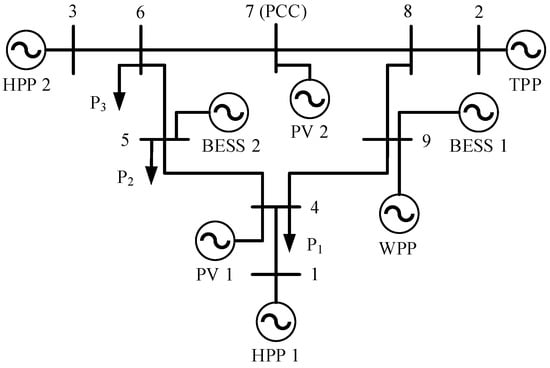
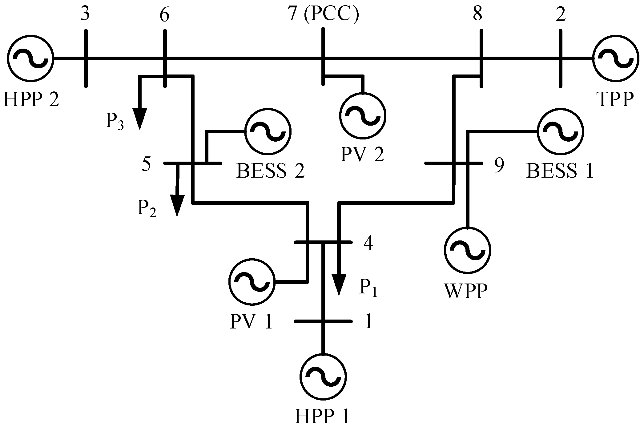
The analysis is conducted on a modified IEEE 9-bus transmission test system that is adapted to represent the operational setting of an energy aggregator. A graphical representation of the network topology is shown in Figure 1.
Figure 1.
Topology of the test system.
The network includes conventional generation from a thermal power plant (TPP), two PV power plants, one WPP, two HPPs and two BESS units. A PCC is placed at node 7. The network topology, transmission line, and load parameters follow [10]; the technical and cost parameters of the generators and renewable units are listed in Table A4, and the battery storage parameters in Table A5, in Appendix A, with the cost values updated for the market conditions of the present study. Generation from RES takes up approximately 74% of installed generation capacity. All market and demand data correspond to a single operating day, 4 November 2025. The hourly day-ahead prices, the contracted day-ahead quantities, and the aggregate demand profile used are listed in Table A1, Table A2 and Table A3 in Appendix A. Day-ahead price data is obtained from the Macedonian electricity market operator MEMO [27], the hourly imbalance (deviation) penalty prices from the Macedonian Transmission System Operator MEPSO [28], and the retail supply price for serving local demand from the Energy and Water Services Regulatory Commission of North Macedonia [29]. The demand follows a typical daily load curve; its hourly values and those of the imbalance penalties for the stated day are available from the cited sources.
Uncertainty in PV output, wind output, and hourly demand is represented by a set of equally probable scenarios, each assigned probability . A convergence study confirming the sufficiency of this count is presented in Section 4.2. Scenarios are generated by applying multiplicative deviations to the deterministic day-ahead forecast of each uncertain quantity. For every scenario, the deviation of quantity x at hour t combines a single per-scenario daily bias , constant across the day, with an hourly fluctuation drawn independently for each hour; the hourly component is smoothed with a three-point moving average to impose temporal correlation between adjacent hours and avoid physically implausible hour-to-hour jumps. The combined deviation is clipped to a bounded range, and the perturbed profile is floored at zero to preclude negative generation or demand:
Demand uses , , and a symmetric bound . PV and wind use larger dispersions, and , with an asymmetric bound that allows availability to fall to zero while limiting upward deviation to of the forecast. All scenarios are drawn with a fixed random seed to ensure reproducibility. The same scenario set is held fixed across all settlement regimes and penalty-multiplier values, so that observed differences are attributable to settlement design rather than to sampling variation.
All optimization runs are executed with the CPLEX MILP solver (Armonk, NY, USA), on an Intel Core i7-9700F workstation (32 GB RAM). Each 200-scenario stochastic MILP involves approximately 379,584 variables and 617,904 constraints; solve times range from 10 to 15 min per run.
4. Results
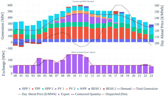
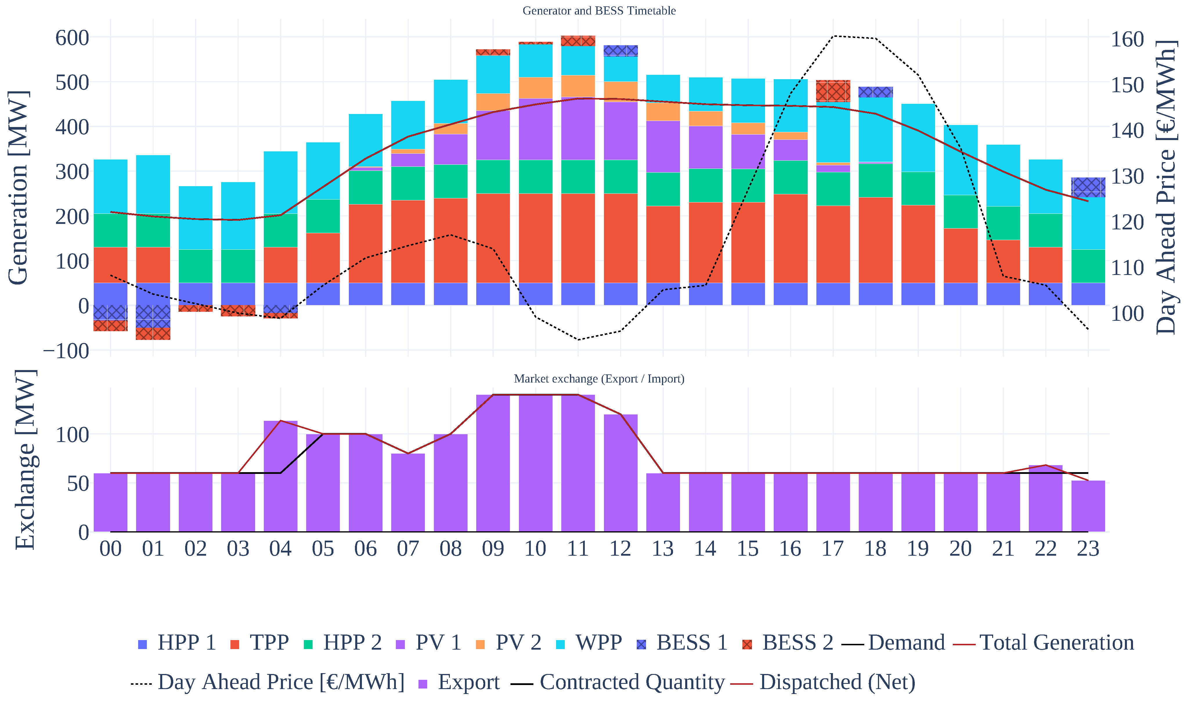
Figure 2 shows the hourly unit commitment and dispatch timetable for the baseline settlement regime (S2) at , for the scenario whose net profit is closest to the expected value of 768,514 € (calculated across all scenarios). This is scenario No. 127, which has an expected profit of 768,836 €, a difference of 322 € compared to the expected profit of the scenario set. Since first-stage commitment decisions are common to all scenarios, the dispatch structure shown is representative of the baseline operating strategy. All subsequent analyses are based on the full distribution of 200 scenarios rather than any single case. From the timetable it can be observed that PV and WPP generation is dispatched at maximum available output throughout the day, reflecting their zero marginal cost. HPP units carry significant load given their low marginal cost relative to the TPP. The TPP is committed during morning and evening peak hours to satisfy demand when renewable availability is lower. BESS units perform intra-day energy shifting, charging during midday solar peaks and discharging during evening demand peaks.
Figure 2.
Hourly dispatch timetable for the baseline settlement regime (S2) at , scenario No.127 with net profit 768,836 €.
The two storage units are identical in rating, efficiency, and degradation cost, differing only in network location (buses 5 and 9). Their dispatch follows conventional intra-day arbitrage, and each cycles the same total energy over the day (91.2 MWh in the scenario shown). The only difference is the particular hours in which each is active; because the units are interchangeable, the optimal aggregate storage trajectory can be split between them in more than one way, so the per-unit allocation carries no significance beyond their combined contribution.
Table 3 presents the key financial risk metrics at the risk-neutral baseline () across all five regimes. Two principal observations emerge.
Table 3.
Financial risk metrics at risk-neutral baseline (, ).
First, removing the contracted position raises profitability while lowering cost. Regimes S4 and S5, which set the contracted day-ahead quantity to zero, avoid the commitment–imbalance cycle that arises when contracted export cannot be delivered in adverse scenarios. Expected cost falls from 478,169 € (S1) to 288,801 € (S4) and 282,955 € (S5), and despite the loss of export revenue the net effect is higher expected profit for S5 (778,284 €), comparable to the liberal regime S1 (782,971 €). Conversely, the strict regime S3 yields the lowest expected profit (744,374 €): the doubled penalty rates make deviations from contracted positions more costly, compelling a more conservative and expensive commitment schedule even under risk-neutral optimization.
Second, tail-risk exposure increases with penalty stringency among the contracted regimes, with CVaR ordered S1 < S2 < S3. The strict regime S3 shows the highest exposure (938,324 €), reflecting the amplification of imbalance costs by doubled penalties in adverse renewable scenarios, while the zero-contract regimes S4 and S5 exhibit the lowest CVaR (455,344 and 431,989 €) by eliminating the variance source associated with contracted market positions. The excess tail-risk ratio rises monotonically with stringency among the contracted regimes (48.6% for S1, 65.2% for S2, and 89.3% for S3), confirming that strict penalties disproportionately inflate tail exposure relative to expected cost; the zero-contract regimes sit between these (57.7% for S4, 52.7% for S5).
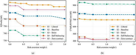
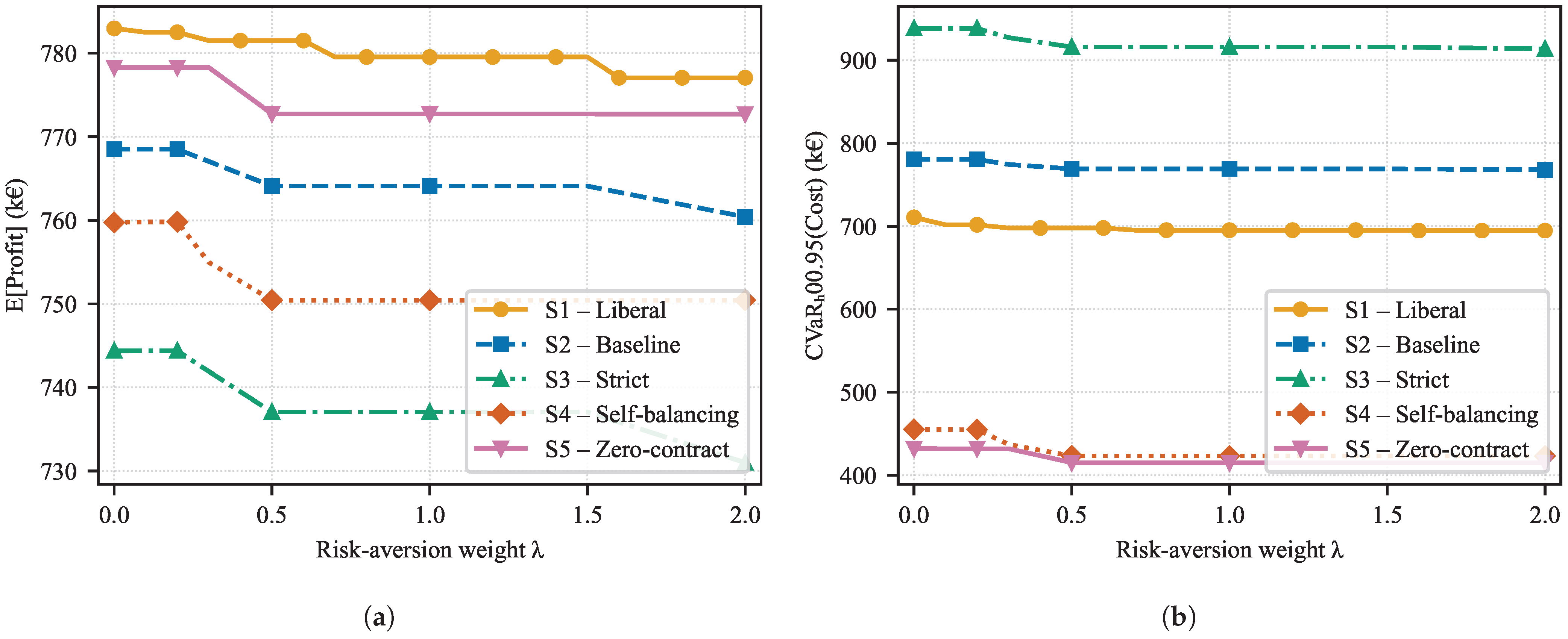
Figure 3 shows the evolution of E[Profit] and CVaRα[Cost] as increases from 0 to 2 for all five regimes.
Figure 3.
Expected profit and CVaR of cost as a function of the risk-aversion weight for all five settlement regimes. (a) Expected profit; (b) CVaR of cost.
All regimes exhibit the same qualitative pattern: CVaRα falls sharply for small and then flattens. Defining the saturation point as the beyond which CVaRα decreases by less than 0.1% per unit increase, the zero-contract regimes saturate earliest ( for both S4 and S5) and the liberal regime shortly after ( for S1), whereas the baseline and strict contracted regimes (S2, S3) continue to yield small CVaR reductions up to the end of the tested range (). The regimes with the least tail risk to remove thus exhaust the available structural adjustments first, while stricter contracted settlement retains a residual benefit from higher risk weights.
At relative to , the absolute CVaR reductions are 15,383 € for S1 (2.2%), 11,486 € for S2 (1.5%), 22,448 € for S3 (2.4%), 32,106 € for S4 (7.1%), and 16,819 € for S5 (3.9%). In absolute terms the reduction is largest for the regimes that start from the highest tail risk relative to their cost base: the zero-contract regime S4 benefits most, and among the contracted regimes the strict regime S3 yields a larger absolute reduction than the liberal S1.
The corresponding expected-profit reductions are 3429 € for S1 (0.4%), 4422 € for S2 (0.6%), 7322 € for S3 (1.0%), 9311 € for S4 (1.2%), and 5545 € for S5 (0.7%). The resulting risk–return efficiency (CVaR reduction per euro of expected profit sacrificed) is high across all regimes, ranging from roughly 2.6 to 4.5, but does not follow a simple monotonic ordering in penalty stringency. This is because the regimes saturate at different risk weights: the liberal regime S1 attains its full available CVaR reduction over a very small profit sacrifice and therefore shows a high ratio, whereas the strict regime S3 is still reducing CVaR at and beyond, so the window understates its total attainable benefit. The robust conclusion is that risk weighting delivers a substantial reduction in tail risk for a small expected-profit cost in every settlement regime, and that the absolute magnitude of that reduction grows with the baseline tail-risk exposure. Table 4 summarizes the key metrics at .
Table 4.
Financial risk metrics at ().
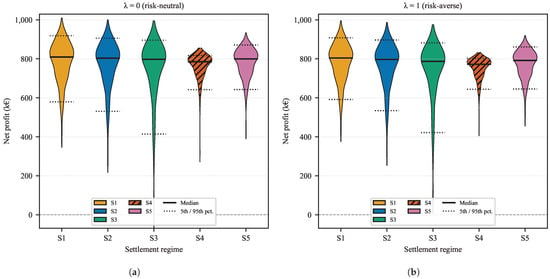
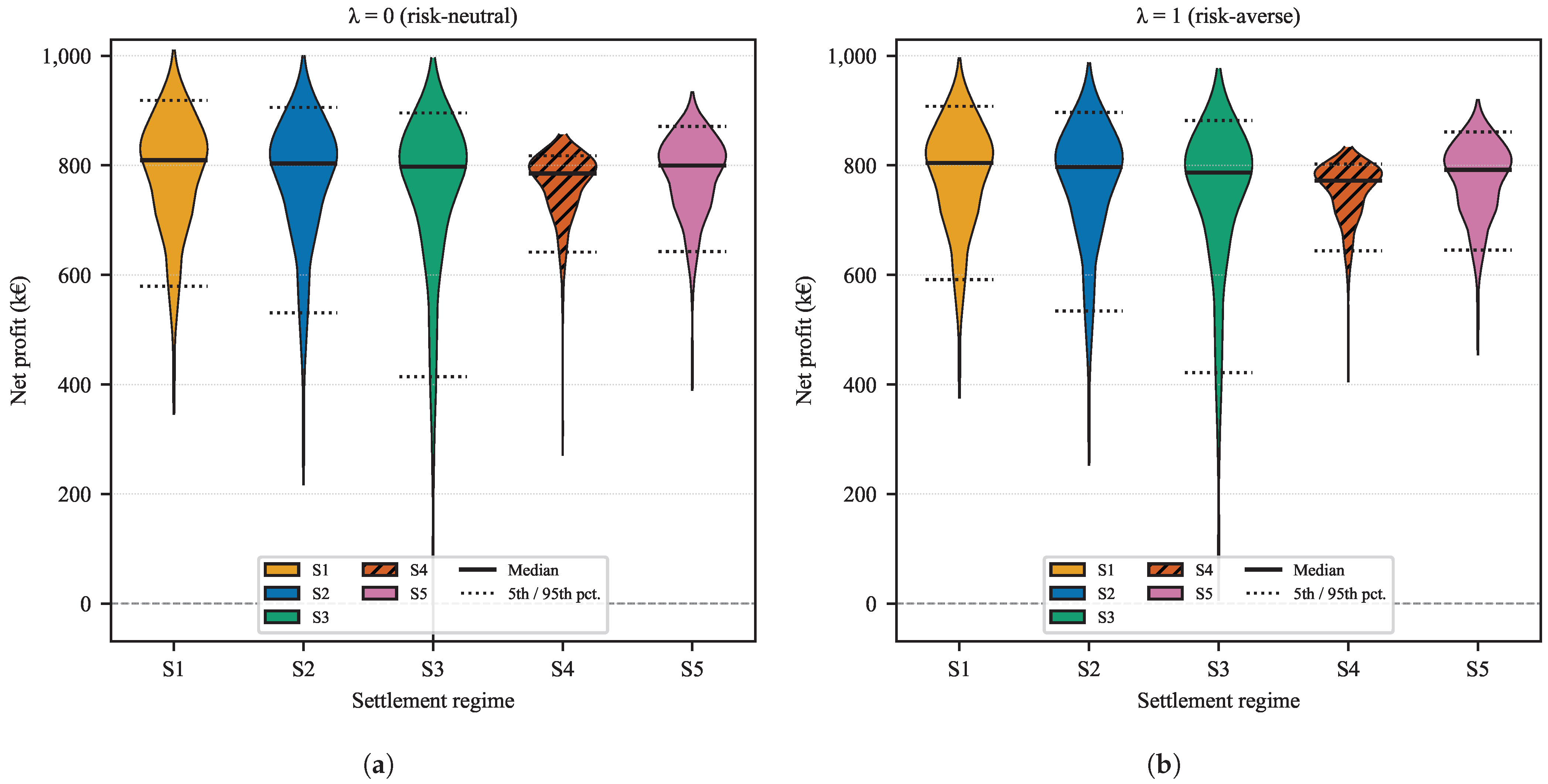
Figure 4 shows the probability-weighted violin plots of the net profit distribution at and for all five regimes.
Figure 4.
Probability-weighted violin plots of per-scenario net profit. Horizontal lines mark the 5th percentile, median, and 95th percentile. (a) Risk-neutral case (); (b) Risk-averse case ().
At , the strict regime S3 exhibits the widest and most left-skewed net-profit distribution, reflecting the amplification of downside outcomes by doubled penalties, while the liberal regime S1 has the narrowest spread. Introducing compresses the lower tail in every regime, most visibly in S3 and in the zero-contract regimes S4 and S5. The compression is achieved by shifting commitment decisions toward greater conservatism, accepting slightly lower median profit in exchange for removing the most extreme losses. In S4 and S5 the distribution at closely mirrors that at except in the lower tail, indicating that risk aversion specifically targets the adverse scenarios associated with high over-delivery penalties.
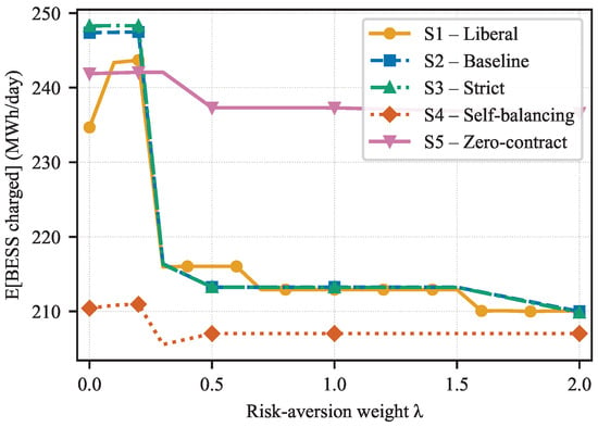
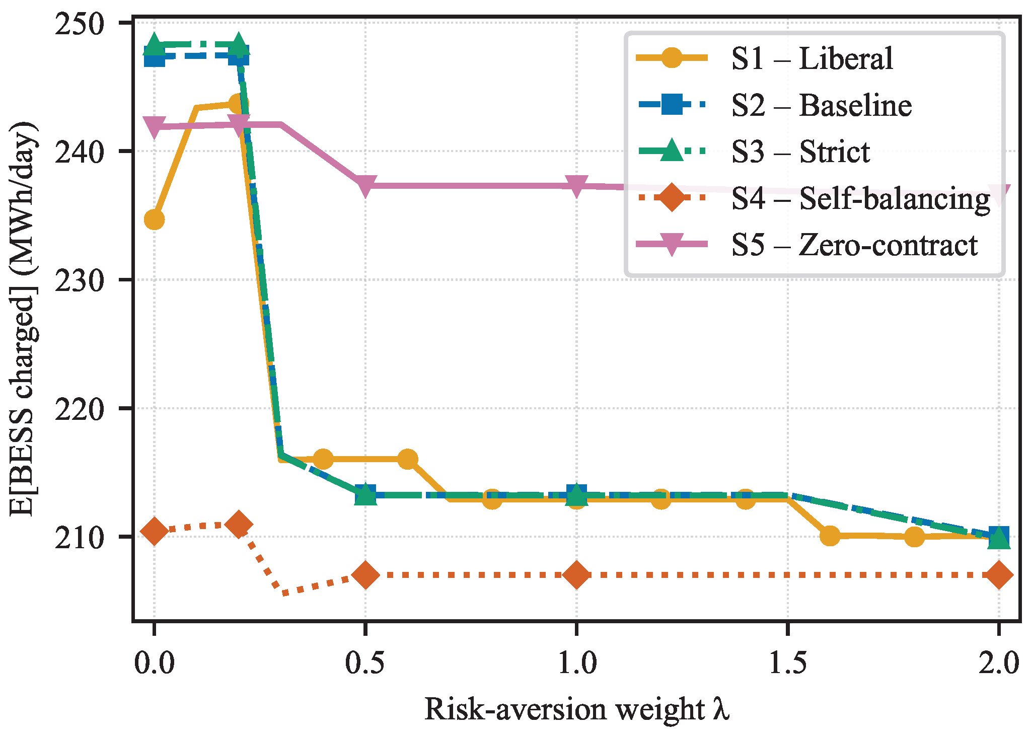
Figure 5 shows the expected BESS energy charged per day as a function of for all five regimes.
Figure 5.
Expected BESS energy charged (MWh/day) as a function of for all five settlement regimes.
For the contracted regimes S1, S2, and S3, BESS throughput decreases with from approximately 235–248 MWh at to a common floor near 213 MWh. The optimizer shifts storage from aggressive energy arbitrage toward a more conservative reserve role, accepting lower expected throughput to reduce exposure to scenarios where arbitrage opportunities fail to materialize.
The zero-contract regimes present a fundamentally different picture: BESS throughput is nearly invariant to , changing by only 3.4 MWh in S4 (210.4 to 207.0) and 4.6 MWh in S5 (241.9 to 237.3), compared with a 22–35 MWh reduction in the contracted regimes. Because S4 and S5 differ only in penalty level (doubled versus baseline) yet both exhibit this invariance, the decoupling is attributable to the removal of the contracted position rather than to penalty stringency. With no contracted exchange, storage is the primary intra-day flexibility resource for matching generation to local demand, so its utilization is set by the load profile and RES availability rather than by risk preferences. The settlement design effectively pre-commits storage to a fixed utilization level that risk weighting cannot override.
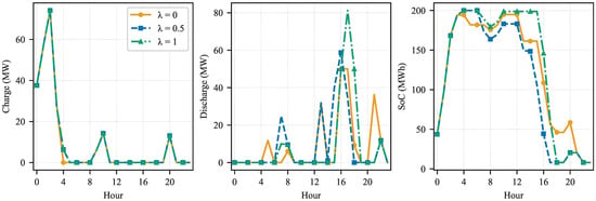
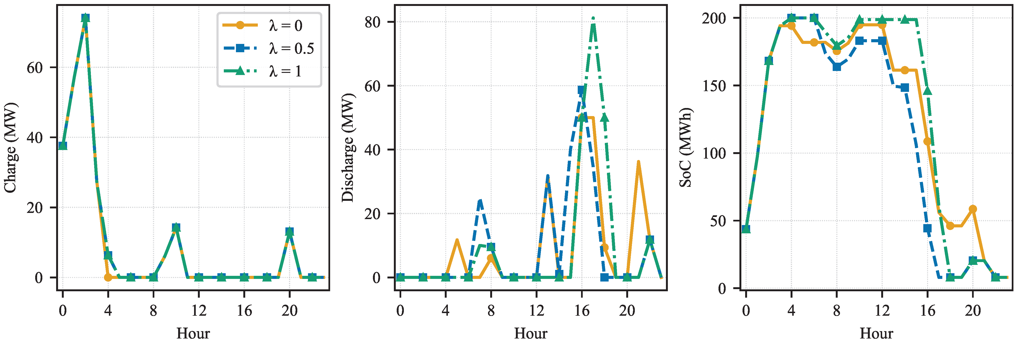
Figure 6 resolves this at the hourly level for the self-balancing regime S4, showing the aggregate charge, discharge, and state-of-charge trajectories at , , and on a common scenario. The daily totals remain relatively unchanged across the three weights, consistent with the throughput invariance reported above. Risk aversion does, however, redistribute storage activity within the day: as increases, discharge is concentrated more tightly around the evening peak (around hour 17) rather than spread across the afternoon and later evening, and the state of charge is held higher through midday before a steeper evening draw-down. Under a zero contracted position the amount of storage cycling is therefore fixed by the demand-matching role and is insensitive to , while the risk weight only reshapes the timing of that cycling, in contrast to the contracted regimes, where higher reduces throughput outright.
Figure 6.
Aggregate hourly BESS operation under the self-balancing regime (S4) at , , and on a common scenario (left to right): charge power; discharge power; state of charge. Daily throughput is nearly invariant to , while the intra-day timing of discharge shifts toward the evening peak as increases.
This finding has practical implications for aggregator technology sizing: in self-balancing environments, the energy throughput that BESS capacity must support is set by the demand-driven flexibility requirement rather than the risk-optimal dispatch strategy. This concerns the throughput (energy) dimension only; a complete sizing study must additionally account for the required power rating and the state-of-charge trajectory, which jointly determine the energy and power capacity of the installation.
A notable and counter-intuitive result across all regimes is that the expected total imbalance penalty increases slightly with rather than decreasing. From to it rises from 18,087 to 19,011 € in S1, 24,449 to 27,485 in S2, 47,462 to 49,617 in S3, 27,627 to 30,570 in S4, and 20,005 to 24,536 in S5.
This arises from the mean–variance trade-off intrinsic to the CVaR objective: to suppress extreme penalties in the worst-case scenarios, the optimizer accepts marginally higher penalties in typical scenarios. The effect is most pronounced in the zero-contract regimes, where the dominant penalty component is over-delivery: in S4 the over-delivery penalty rises from 25,041 to 29,665 € while the shortfall component falls from 2585 to 905 €, and S5 shows the same pattern (over-delivery 18,721 to 24,073 €, shortfall 1285 to 462 €). Under a zero contracted position, risk-averse scheduling commits more conservative generation to avoid shortfall, which in turn raises over-delivery in high-renewable scenarios.
4.1. Continuous Penalty-Multiplier Sweep
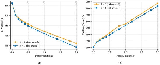
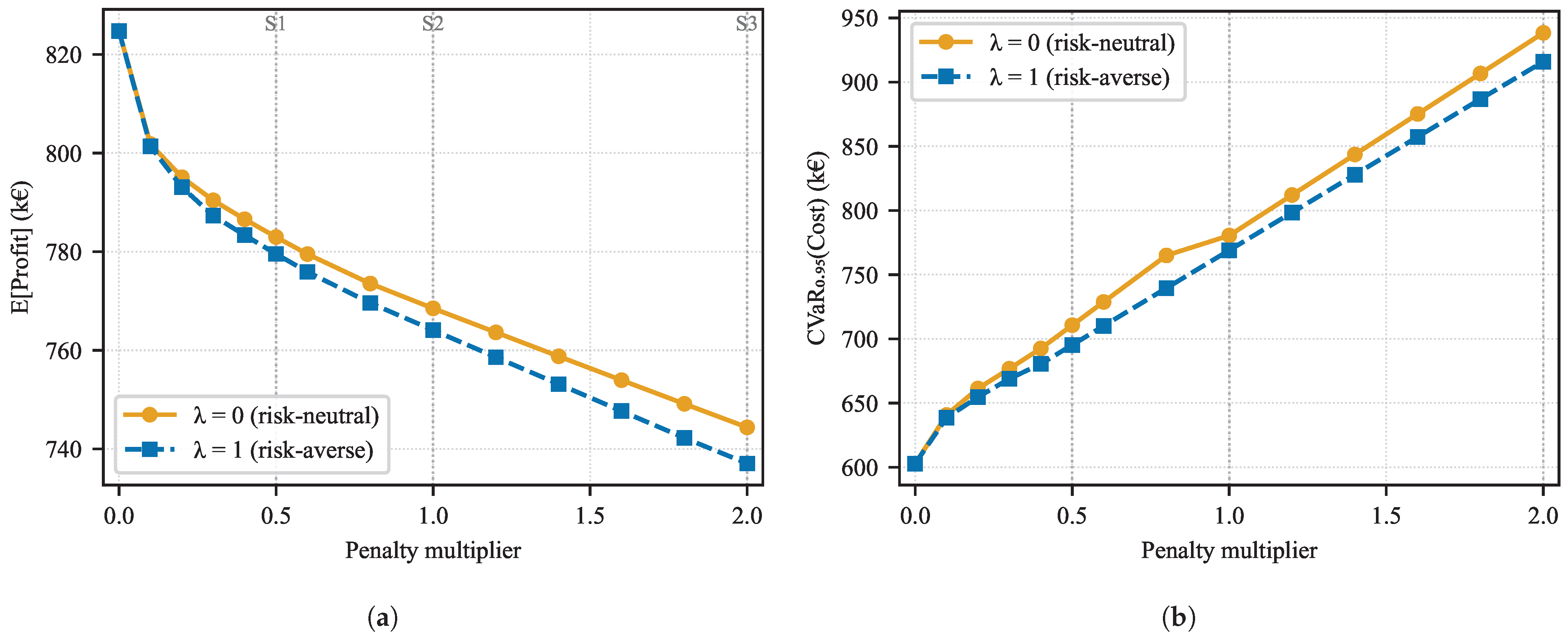
Figure 7 and Figure 8 present a continuous sweep of the penalty multiplier over [0, 2.0] at and . The multipliers 0.5, 1.0, and 2.0 reproduce the S1, S2, and S3 penalty profiles exactly, and the corresponding sweep values coincide with those of Table 3, confirming that the discrete regimes are points on a single continuous curve.
Figure 7.
Expected profit and CVaR of cost as a function of the penalty multiplier, for and . Vertical marks indicate the multipliers reproducing regimes S1, S2, and S3. (a) Expected profit; (b) CVaR of cost.
Figure 8.
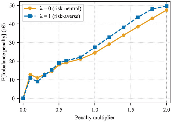
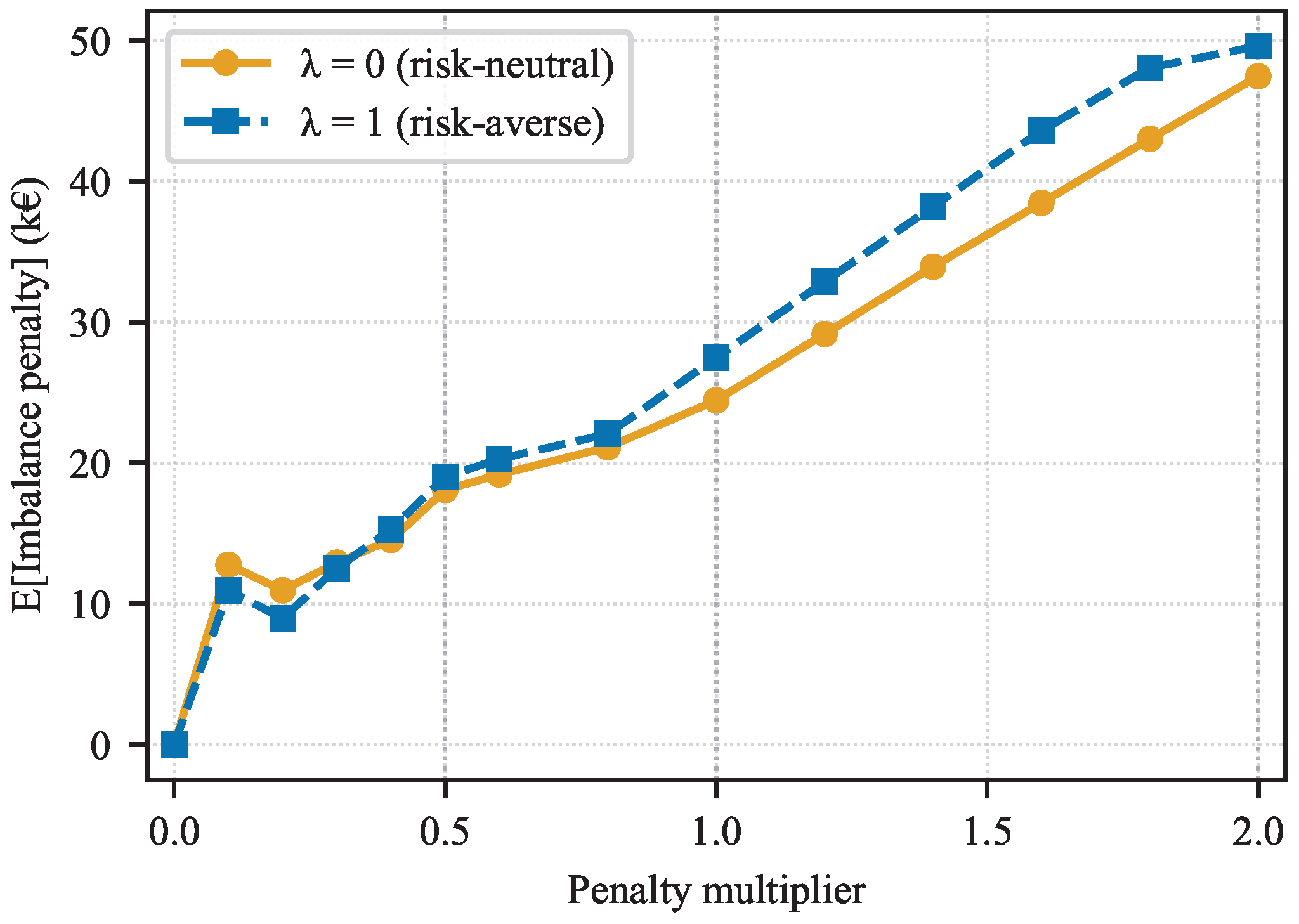
Expected total imbalance penalty as a function of the penalty multiplier, for and . Vertical marks indicate the multipliers reproducing regimes S1, S2, and S3.
Expected profit falls sharply as the multiplier rises from zero, reflecting the onset of imbalance settlement, and then declines steadily, from 824,732 € at a zero multiplier to 744,377 € at a multiplier of 2.0 (), the latter coinciding with the strict regime S3. CVaR(cost) rises monotonically, and beyond a multiplier of approximately 0.3 the increase is close to linear, at roughly 151,000 € per unit multiplier for and 147,000 € for . This near-linearity indicates that the settlement-induced deviation volume remains approximately constant across the tested range: the optimizer absorbs stricter penalties as higher settlement cost rather than restructuring its commitment to eliminate the underlying deviations.
The two risk-aversion weights separate as stringency increases: at a unit multiplier, risk aversion reduces CVaR by 11,486 € for a 4420 € reduction in expected profit, while at a doubled multiplier it reduces CVaR by 22,448 € for a 7325 € profit sacrifice. The absolute tail-risk reduction available from risk weighting thus grows with settlement stringency, consistent with the regime-level findings.
Figure 8 shows expected imbalance penalty against the multiplier. For multipliers of 0.3 and above, the risk-averse schedule () incurs a higher expected penalty than the risk-neutral one, rising in parallel with it—the mean-for-variance trade characteristic of the CVaR objective, which accepts marginally higher typical-case penalties to suppress tail outcomes. At the lowest non-zero multipliers (up to 0.3) the ordering reverses and the curve is non-monotonic; this reflects near-degenerate first-stage commitment decisions in the regime—where the penalty term carries little weight and where the solver selects among near-optimal schedules at adjacent multiplier values—and should not be read as a structural reversal.
4.2. Scenario Convergence
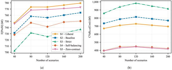
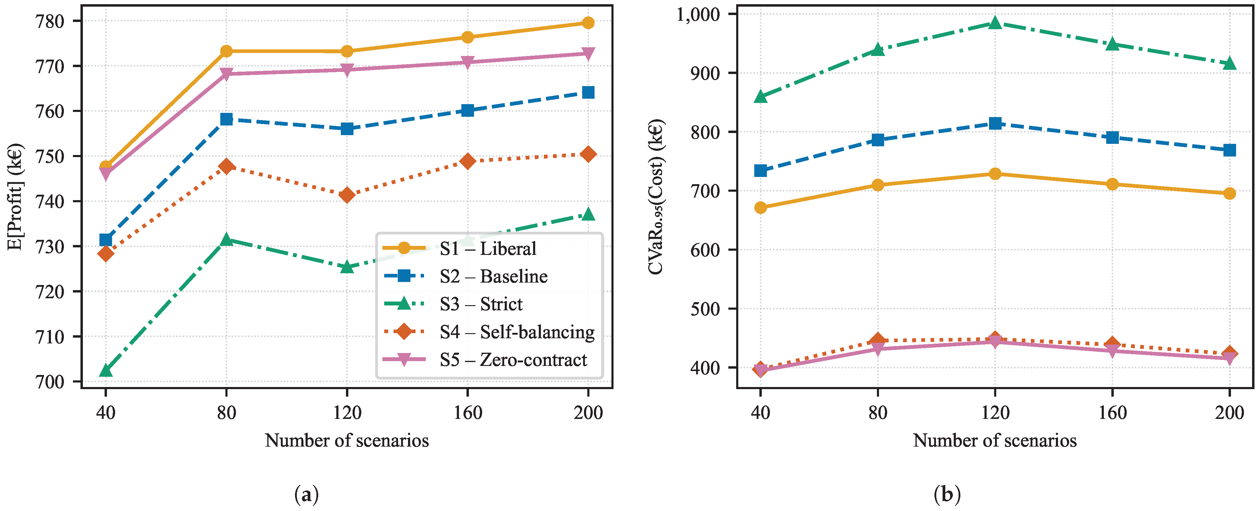
To verify that the 200-scenario set is sufficient to resolve the reported metrics and, in particular, that the regime comparisons are not an artifact of sampling, the full five-regime analysis was repeated at for scenario counts of 40, 80, 120, 160, and 200. The scenario sets are nested (each larger set contains all scenarios of the smaller ones, generated from the same seed), so the trajectories isolate the effect of adding scenarios rather than resampling. The risk-averse weight is used throughout, as it activates the CVaR term and therefore places the greatest demand on the tail estimate; convergence of the risk-neutral case () is at least as fast, since it does not depend on the tail.
Figure 9 shows the behaviour of expected profit and CVaR(cost) as the scenario count increases. Expected profit stabilizes quickly: beyond 120 scenarios the change in each regime is below 1% of the final value (0.25–1.0% from 160 to 200 scenarios), and the ordering of the regimes by expected profit is identical at every scenario count. CVaR(cost), being a tail quantity, converges more slowly and retains a small residual variation: the change from 160 to 200 scenarios is 2.5–4.0% of the final value, with successive increments diminishing but not strictly monotone, as expected for a 5%-tail estimate drawn from a few hundred scenarios. The rank ordering of the regimes by CVaR is invariant across all tested counts (S5 < S4 < S1 < S2 < S3), as is the ordering by expected profit (S3 < S4 < S2 < S5 < S1). The absolute metrics therefore exhibit at most a few per cent of sampling variation at 200 scenarios, while the comparative findings on which the paper’s conclusions rest are stable with respect to the scenario count.
Figure 9.
Convergence of the reported metrics with scenario count, at , for all five settlement regimes. (a) Expected profit; (b) CVaR of cost.
4.3. Confidence-Level Sensitivity
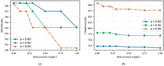
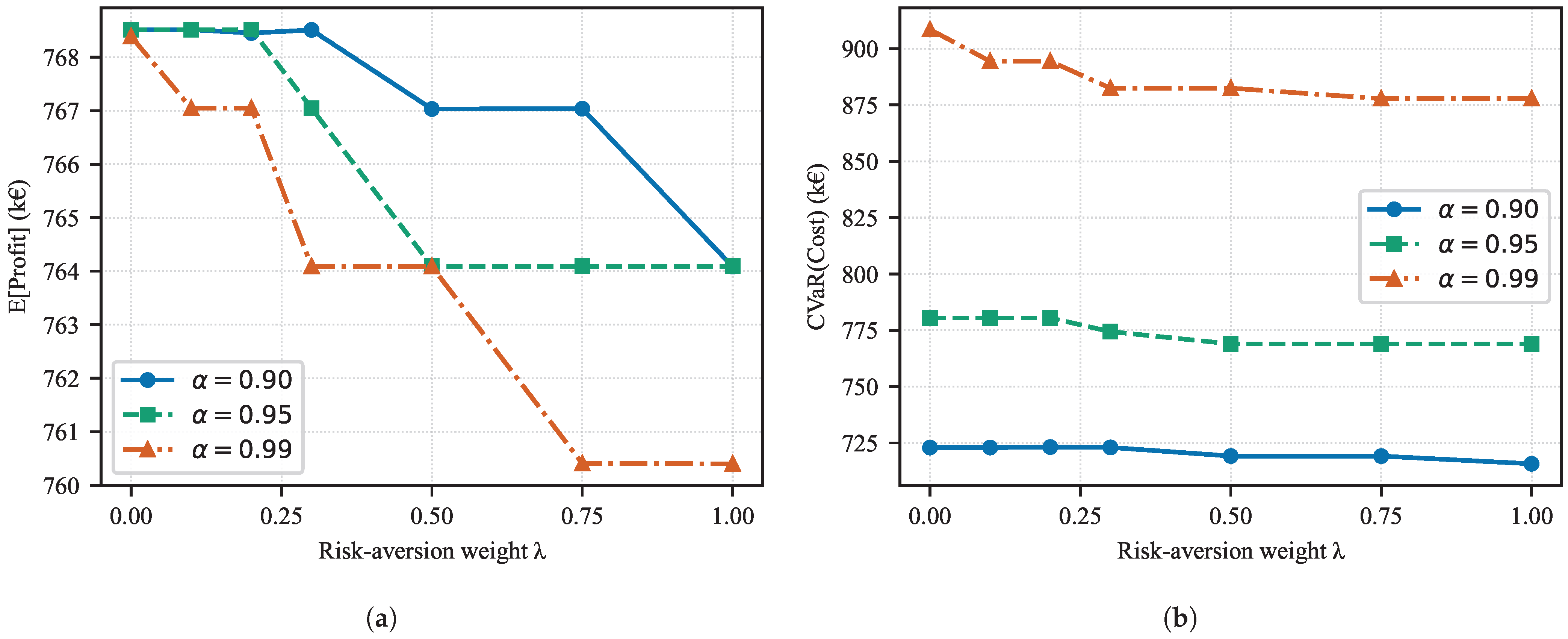
The settlement-regime analysis above fixes the CVaR confidence level at . Because the study characterizes tail-risk behaviour, the choice of could in principle influence both the optimal schedule and the saturation of the risk-aversion weight. To assess this, the baseline regime (S2) -sweep was repeated at , , and . Figure 10 shows the resulting expected profit and CVaR of cost as functions of for the three confidence levels.
Figure 10.
Sensitivity of the baseline regime (S2) to the CVaR confidence level , as a function of the risk-aversion weight . (a) Expected profit; (b) CVaR of cost.
As expected, a higher confidence level targets a thinner tail: the risk-neutral () CVaR of cost rises from approximately 723,000 € at to 780,000 € at and 908,000 € at . The expected-profit cost of risk aversion grows correspondingly, from 0.58% of the risk-neutral profit over the full range at and to 1.04% at .
The saturation behaviour of the risk-aversion weight is robust to this choice. At every confidence level, CVaR falls steeply for small and then saturates, with the location of the saturation point shifting only modestly, from at to at . Beyond no further tail-risk reduction is obtained: the CVaR values are unchanged between and at both and . The conclusion that a moderate risk weight captures essentially the entire available tail-risk reduction therefore holds across confidence levels, with the quantitative effect of on the targeted tail region consistent with the detailed treatment in [10].
4.4. Policy Implications
Three policy-relevant conclusions emerge from the combined results.
First, settlement design is a principal determinant of baseline tail-risk exposure. Even before any risk aversion is applied, CVaR rises from 710,631 € under the liberal regime (S1) to 938,324 € under the strict regime (S3), a 32% increase for a doubling of penalty rates, and the continuous sweep shows this exposure growing almost linearly with penalty stringency rather than saturating. More tellingly, the excess tail-risk ratio climbs from 49% to 89% over the same range, so stricter penalties inflate tail risk disproportionately relative to expected cost. Regulators designing settlement mechanisms should be aware that the optimizer cannot fully hedge these amplified costs through scheduling adjustments alone.
Second, risk-based scheduling delivers a favourable risk–return trade in every settlement regime, and its absolute value grows with baseline tail-risk exposure. At , risk weighting reduces CVaR by between 1.5% and 7.1% for an expected-profit sacrifice of at most about 1.2%, with the largest absolute reductions in the regimes that start from the highest tail risk. A moderate weight is sufficient to capture most of the available benefit: the zero-contract and liberal regimes saturate near –, while the baseline and strict contracted regimes continue to benefit from higher weights. Aggregators should therefore scale their risk weight to the tail-risk exposure implied by the prevailing settlement design rather than apply a single fixed value.
Third, self-balancing constraints decouple the volume of storage cycling from risk preferences. Under a zero contracted position, daily BESS throughput is fixed by the demand-matching role and is nearly invariant to ; risk aversion reshapes only the intra-day timing of charging and discharging, not the total energy cycled (Figure 6). Aggregators operating under self-balancing rules therefore cannot use to modulate the amount of BESS utilization, although it still influences when storage is dispatched within the day. Consequently, BESS sizing (which depends on cycled energy rather than its timing) must be determined from the structural demand-matching role, and the co-optimization of risk-aversion strategy with storage sizing is most meaningful for aggregators that retain market participation rights. This sizing guidance should be read as first-order: the degradation cost here is a throughput-linear operating term applied identically across regimes, and a cycle-resolved model capturing depth-of-discharge, state-of-charge, and temperature-dependent aging would be required for detailed lifetime or warranty-level storage assessment, as noted in Section 5.
5. Discussion
The proposed framework provides a single, internally consistent environment in which the effect of imbalance settlement design on risk-averse aggregator scheduling can be isolated. Because all five regimes share the same portfolio, network model, and scenario set, the observed differences in expected profit, tail risk, storage utilization, and penalty exposure are attributable to settlement design alone. The continuous penalty-multiplier sweep further resolves the discrete regimes as points on a single curve, giving a quantitative rather than categorical view of how stringency shapes the risk–return tradeoff. Beyond scheduling, the results serve a diagnostic purpose, indicating which flexibility resources absorb uncertainty at each level of risk aversion and how that role changes once the contracted market position is removed.
As an analysis built on an established modeling framework rather than a new solution algorithm, the study is validated through internal consistency and provenance rather than against field measurements. The underlying stochastic UC/CVaR engine is the peer-reviewed formulation of the companion study [10], reused here without modification. The discrete settlement regimes and the continuous penalty-multiplier sweep are produced by two independent configurations of the same model, and they coincide exactly at the multipliers that reproduce the S1, S2, and S3 penalty profiles, confirming internal consistency. The analysis is conducted on the modified IEEE 9-bus system, a widely adopted benchmark that keeps the setup reproducible and comparable with related work. Finally, the qualitative behavior matches theoretical expectations: CVaR rises monotonically with penalty stringency, risk weighting reduces tail risk at a small expected-profit cost, and the two electrically identical storage units cycle equal total energy. The comparative findings are robust to the scenario sample: a convergence study (Section 4.2) shows that, although the absolute profit and CVaR values retain a few per cent of sampling variation at 200 scenarios, the ordering of regimes by both expected profit and tail risk is invariant across scenario counts from 40 to 200.
Several limitations should be stated plainly. The study compares the five settlement regimes under a single, fixed set of operating conditions (one representative day of demand, renewable availability, and market prices on a transmission-level benchmark with a linearized network and voltage representation). Holding these conditions constant across all regimes is what isolates the effect of settlement design, and is therefore a deliberate scope choice rather than a data constraint; the comparative relationships reported here are structural and do not depend on the particular day, although the absolute profit and cost levels naturally do. By the same token, the main regime comparison uses the CVaR risk measure at a single confidence level (), with robustness to this choice examined in Section 4.3, and the scenario set, although enlarged to 200 samples, rests on a parametric Gaussian error model rather than field-derived forecast errors and a single random seed, so the tail estimates carry sampling variability that is largest at , where the conditional average is taken over only the worst 1% of scenarios. These choices are appropriate for a controlled comparative study but limit direct transfer to field operation. The conclusions are limited to the modified IEEE 9-bus network studied, and the sensitivity of the results to relaxing individual network limits has not been evaluated. Future work will characterize how the settlement effect itself varies across multiple representative days, seasons, and renewable-penetration levels; address multi-period and rolling-horizon scheduling, the joint optimization of storage sizing with the risk-aversion strategy, and validation on a distribution-level aggregator network with higher R/X ratios; and compare against alternative uncertainty distributions and risk measures such as distributionally robust or chance-constrained formulations. The battery degradation cost is modeled as a linear function of energy throughput, which captures the first-order cost of cycling but not depth-of-discharge, state-of-charge, or temperature-dependent aging effects; incorporating a nonlinear, cycle-resolved degradation model [21] is a worthwhile refinement left to future work, although it is not expected to alter the settlement-regime comparison, since the same degradation cost applies across all regimes. Relatedly, the present study addresses financial and operational risk only; the physical safety risks of large-scale battery storage, such as thermal runaway and its propagation, are a distinct and important concern documented in the dedicated safety literature [30,31].
6. Conclusions
This paper has studied how imbalance settlement design shapes the risk–return tradeoff for a network-constrained energy aggregator, using a risk-based stochastic unit commitment framework applied to a modified IEEE 9-bus test system across five settlement regimes and a parametric sweep from 0 to 2.
At the risk-neutral baseline, stricter penalty rates substantially increase CVaR without a proportional increase in expected cost, with the excess tail-risk ratio reaching 89% under doubled penalties compared to 49% under liberal settlement. The zero-contract regimes yield the lowest tail risk and, in the baseline-penalty case (S5), an expected profit comparable to the liberal regime, by removing the contracted position and settling all exchange as imbalance—at the cost of structural inflexibility.
Across all regimes CVaR falls steeply for small and then flattens; the zero-contract and liberal regimes saturate near –, while the baseline and strict contracted regimes retain a residual benefit up to . Risk weighting reduces tail risk by 1.5–7.1% for an expected-profit cost of at most about 1.2%, with the largest absolute reductions where baseline tail risk is highest. Under the zero-contract regimes, BESS throughput changes by under 5 MWh/day across the full range, compared with a 22–35 MWh/day reduction in the contracted regimes, becoming effectively invariant to . The continuous penalty-multiplier sweep confirms that tail-risk exposure scales almost linearly with settlement stringency because the underlying deviation volume remains approximately fixed across the tested range. These comparative conclusions are stable with respect to the scenario count (Section 4.2), and the saturation of the risk-aversion weight is robust to the CVaR confidence level (Section 4.3).
The practical implication is that aggregators should calibrate their risk weight jointly with the prevailing settlement regime: a moderate weight () captures most of the available benefit in the zero-contract and liberal regimes, while stricter contracted settlement rewards somewhat higher weights.
Author Contributions
Conceptualization, P.P.; methodology, P.P.; software, P.P.; validation, P.P., G.V., M.A., S.N.P. and A.C.; formal analysis, P.P. and G.V.; investigation, P.P.; resources, P.P.; data curation, P.P. and G.V.; writing—original draft preparation, P.P.; writing—review and editing, P.P.; visualization, P.P.; supervision, P.P., G.V., M.A., S.N.P. and A.C.; project administration, P.P. All authors have read and agreed to the published version of the manuscript.
Funding
This research received no external funding.
Data Availability Statement
Data will be made available upon request.
Acknowledgments
During the preparation of this work, the authors used Claude Opus 4.8 (Anthropic, San Francisco, CA, USA), in order to assist with text refinement and language editing. After using this tool, the authors reviewed and edited the content as needed and take full responsibility for the content of the publication.
Conflicts of Interest
The authors declare no conflicts of interest.
Abbreviations and Nomenclature
The following abbreviations and nomenclature are used in this manuscript:
| BESS | Battery energy storage systems |
| CVaR | Conditional value-at-risk |
| DER | Distributed energy resource |
| DA | Day-ahead |
| ED | Economic dispatch |
| GGDF | Generalized generation distribution factor |
| HPP | Hydro power plant |
| MILP | Mixed-integer linear program |
| MVA | Megavolt-Amperes |
| MW | Megawatt |
| MWh | Megawatt-hour |
| PCC | Point of common coupling |
| PV | Photovoltaic |
| p.u. | Per-unit |
| RES | Renewable energy sources |
| SOC | State of charge |
| SUC | Stochastic unit commitment |
| TPP | Thermal power plant |
| UC | Unit commitment |
| VTDF | Voltage transfer distribution factor |
| WPP | Wind power plant |
| The following nomenclature is used in this manuscript: | |
| Indices and sets | |
| s | Scenario index, |
| i | Dispatchable generator index |
| e | BESS unit index |
| w | Wind power plant index |
| p | PV power plant index |
| l | Transmission line index |
| n | Bus index |
| t | Hour index, |
| Cardinalities | |
| S | Total number of scenarios |
| T | Scheduling horizon (hours) |
| Number of dispatchable generators | |
| Number of emitting units | |
| Number of BESS units | |
| Number of wind power plants | |
| Number of PV power plants | |
| Number of buses | |
| First-stage decision variable | |
| Binary commitment status of generator i at hour t | |
| Second-stage decision variables | |
| Active power output of generator i [MW] | |
| Wind generation dispatch [MW] | |
| Solar PV generation dispatch [MW] | |
| BESS charging power [MW] | |
| BESS discharging power [MW] | |
| Binary charging status indicator | |
| Binary discharging status indicator | |
| State of charge of BESS unit e [MWh] | |
| Net power injection at bus n [MW] | |
| Energy not served [MW] | |
| Over-delivery deviation from contracted quantity [MW] | |
| Shortfall deviation from contracted quantity [MW] | |
| CVaR auxiliary variables | |
| VaR proxy (lower bound on the -quantile) | |
| Excess cost above in scenario s | |
| Cost and market parameters | |
| Probability of scenario s | |
| CVaR confidence level | |
| Risk-aversion weight | |
| Total operating cost in scenario s | |
| Generation cost of unit i [€] | |
| Marginal degradation cost of BESS unit e [€/MWh] | |
| Carbon emission price [€/tCO2] | |
| ENS penalty price [€/MWh] | |
| Start-up cost of unit i at hour t [€] | |
| Contracted day-ahead quantity at hour t [MWh] | |
| Day-ahead market price at hour t [€/MWh] | |
| Retail supply tariff at hour t [€/MWh] | |
| Over-delivery imbalance penalty [€/MWh] | |
| Shortfall imbalance penalty [€/MWh] | |
| Technical parameters | |
| Emission factor of unit i [tCO2/MWh] | |
| Minimum and maximum active power output of unit i [MW] | |
| Minimum and maximum state of charge of BESS unit e [MWh] | |
| Charging efficiency of BESS unit e | |
| Discharging efficiency of BESS unit e | |
| Thermal capacity limit of line l [MW] | |
| GGDF matrix | |
| Scenario-dependent maximum available PV output [MW] | |
| Scenario-dependent maximum available wind output [MW] | |
| Net grid demand in scenario s at hour t [MW] | |
Appendix A. Hourly Input Data and Specifications
This appendix reports the deterministic hourly input data for the operating day (4 November 2025), provided to support reproducibility. Table A1 gives the demand of each load (P1 at bus 4, P2 at bus 5, P3 at bus 6), Table A2 the available output of each renewable plant (PV 1 at bus 4, PV 2 at bus 7, and the wind plant WPP at bus 9), and Table A3 the market inputs common to all settlement regimes. Renewable availability is the hourly upper bound on dispatch. The demand and renewable profiles listed here are the nominal profiles around which the 200 scenarios are generated, following the procedure in Section 3. In Table A3, the penalty prices are the baseline (S2) values, scaled by in S1 and in S3 and S4; the contracted quantity is set to zero in regimes S4 and S5. The retail tariff is 129 EUR/MWh in all hours.
Table A1.
Hourly demand per load point [MW].
Table A2.
Hourly renewable availability (upper bound on dispatch) per plant.
Table A3.
Hourly market inputs, common to all settlement regimes.
Table A4.
Generator and renewable unit specifications.
Table A5.
Battery energy storage specifications (both units identical).
References
- Kerscher, S.; Arboleya, P. The key role of aggregators in the energy transition under the latest European regulatory framework. Int. J. Electr. Power Energy Syst. 2021, 134, 107361. [Google Scholar] [CrossRef] [Scilit]
- Da Costa, V.B.F.; de Doile, G.N.D.; Troiano, G.; Dias, B.H.; Bonatto, B.D.; Soares, T.; de Freitas Filho, W. Electricity Markets in the context of Distributed Energy Resources and Demand Response Programs: Main developments and challenges based on a systematic literature review. Energies 2022, 15, 7784. [Google Scholar] [CrossRef] [Scilit]
- Brusco, G.; Menniti, D.; Sorrentino, N. A rolling horizon management model to reduce imbalance in real-time for a renewable energy community. Sustain. Energy Grids Netw. 2025, 43, 101828. [Google Scholar] [CrossRef] [Scilit]
- Algarvio, H.; Couto, A.; Estanqueiro, A. A Double Pricing and Penalties ‘Separated’ Imbalance Settlement Mechanism to Incentive Self Balancing of Market Parties. In Proceedings of the 20th International Conference on the European Energy Market (EEM), Istanbul, Turkey, 10–12 June 2024; pp. 1–6. [Google Scholar] [CrossRef] [Scilit]
- Huang, Y.; Zheng, Q.P.; Wang, J. Two-stage stochastic unit commitment model including non-generation resources with conditional value-at-risk constraints. Electr. Power Syst. Res. 2014, 116, 427–438. [Google Scholar] [CrossRef] [Scilit]
- Mahmutoğulları, A.İ.; Ahmed, S.; Çavuş, Ö.; Aktürk, M.S. The Value of Multi-Stage Stochastic Programming in Risk-Averse Unit Commitment Under Uncertainty. IEEE Trans. Power Syst. 2019, 34, 3667–3676. [Google Scholar] [CrossRef] [Scilit]
- Constante-Flores, G.E.; Conejo, A.J.; Lima, R.M. Stochastic scheduling of generating units with weekly energy storage: A hybrid decomposition approach. Int. J. Electr. Power Energy Syst. 2022, 145, 108613. [Google Scholar] [CrossRef] [Scilit]
- Yang, C.; Sun, W.; Yang, J.; Han, D. Risk-averse two-stage distributionally robust economic dispatch model under uncertain renewable energy. CSEE J. Power Energy Syst. 2024, 10, 1514–1524. [Google Scholar] [CrossRef] [Scilit]
- Herre, L. Impact of Imbalance Settlement System Design on Risk-Averse Energy Storage. In Proceedings of the 17th International Conference on the European Energy Market (EEM), Stockholm, Sweden, 16–18 September 2020; pp. 1–6. [Google Scholar] [CrossRef] [Scilit]
- Popovski, P.; Veljanovski, G.; Atanasovski, M.; Nikolova Poceva, S.; Chaushevski, A. Conditional Value-at-Risk Optimization in Stochastic Unit Commitment for Energy Aggregator Scheduling. Energies 2026, 19, 3874. [Google Scholar] [CrossRef] [Scilit]
- Latify, M.A.; Mokhtari, A.; Alavi-Eshkaftaki, A.; Rajaei Najafabadi, F.; Hashemian, S.N.; Khaleghizadeh, A.; Nezamabadi, H.; Yousefi Ramandi, M.; Mozdawar, S.A.; Hatziargyriou, N.D.; et al. Security-constrained unit commitment: Modeling, solutions and evaluations. Appl. Energy 2025, 390, 125796. [Google Scholar] [CrossRef] [Scilit]
- Kaewpasuk, S.; Intiyot, B.; Jeenanunta, C. A Two-Stage Stochastic Unit Commitment Model for Sustainable Large-Scale Power System Planning under Renewable and EV Variability. Energies 2025, 18, 4614. [Google Scholar] [CrossRef] [Scilit]
- Malamaki, K.-N.D.; Fotopoulou, M.; Martinez-Lopez, D.; Lampsidis, G.; Ferrer-Fernandez, P.; Andriopoulos, N.; Tzanis, N.; Kaousias, K.; Chassioti, E.; Moraitis, I. Day ahead optimization of insular systems considering future interconnection: The case of Ikaria island. Sustain. Energy Grids Netw. 2025, 44, 102018. [Google Scholar] [CrossRef] [Scilit]
- Asensio, M.; Contreras, J. Stochastic unit commitment in isolated systems with renewable penetration under CVaR assessment. IEEE Trans. Smart Grid 2016, 7, 1356–1367. [Google Scholar] [CrossRef] [Scilit]
- Moreira, A.; Fanzeres, B.; Silva, P.; Heleno, M.; Marcato, A.L.M. On the role of Battery Energy Storage Systems in the day-ahead Contingency-Constrained Unit Commitment problem under renewable penetration. Electr. Power Syst. Res. 2024, 235, 110856. [Google Scholar] [CrossRef] [Scilit]
- Fazlhashemi, S.S.; Khodayar, M.E.; Sedighizadeh, M.; Khodayar, M. Risk-averse operation of microgrids in distribution systems with price-responsive demands. Int. J. Electr. Power Energy Syst. 2025, 168, 110581. [Google Scholar] [CrossRef] [Scilit]
- Datta, J.; Das, D. Risk-constrained energy management of multi-energy multi-microgrids system with integrated demand response using hybrid risk assessment approach. Energy 2025, 331, 136638. [Google Scholar] [CrossRef] [Scilit]
- Nobis, M.; Schmitt, C.; Schemm, R.; Schnettler, A. Pan-European CVaR-Constrained Stochastic Unit Commitment in Day-Ahead and Intraday Electricity Markets. Energies 2020, 13, 2339. [Google Scholar] [CrossRef] [Scilit]
- Mirzaei, M.A.; Ahmadian, A.; Mohammadi-Ivatloo, B.; Zare, K.; Elkamel, A. A mixed conditional value-at-risk/information gap decision theory framework for optimal participation of a multi-energy distribution system in multiple energy markets. J. Clean. Prod. 2022, 371, 133283. [Google Scholar] [CrossRef] [Scilit]
- Xiang, Z.; Huang, C.; Li, K.; Wang, C.; Siano, P. A risk-aware coordinated trading strategy for load aggregators with energy storage systems in the electricity spot market and demand response market. iEnergy 2025, 4, 31–42. [Google Scholar] [CrossRef] [Scilit]
- Camuñas García-Miguel, P.L.; Alonso-Martinez, J.; Arnaltes Gómez, S.; Rodríguez-Amenedo, J.L. Impact of risk measures and degradation cost on the optimal arbitrage schedule for battery energy storage systems. Int. J. Electr. Power Energy Syst. 2024, 157, 109883. [Google Scholar] [CrossRef] [Scilit]
- Xiao, D. A Review on Risk-Averse Bidding Strategies for Virtual Power Plants with Uncertainties: Resources, Technologies, and Future Pathways. Technologies 2025, 13, 488. [Google Scholar] [CrossRef] [Scilit]
- Zheng, Y.; Wang, Y.; Yang, Q. Bidding strategy design for electric vehicle aggregators in the day-ahead electricity market considering price volatility: A risk-averse approach. Energy 2023, 283, 129138. [Google Scholar] [CrossRef] [Scilit]
- Mujeeb, A.; Hu, Z.; Wang, J.; Diao, R.; Liu, L.; Bao, Z. Optimizing Virtual Power Plant Operations in Energy and Frequency Regulation Reserve Markets: A Risk-Averse Two-Stage Scenario-Oriented Stochastic Approach. Int. Trans. Electr. Energy Syst. 2025, 2025, 6640754. [Google Scholar] [CrossRef] [Scilit]
- Ioannidis, F.; Georgitsioti, T.; Kosmidou, K.; Zopounidis, C.; Andriosopoulos, K. A simulation model for imbalance costs of renewable energy aggregators: The case of Greek balancing market. Energy Econ. 2025, 142, 108155. [Google Scholar] [CrossRef] [Scilit]
- Klyve, Ø.S.; Klæboe, G.; Nygård, M.M.; Marstein, E.S. Limiting imbalance settlement costs from variable renewable energy sources in the Nordics: Internal balancing vs. balancing market participation. Appl. Energy 2023, 350, 121696. [Google Scholar] [CrossRef] [Scilit]
- Macedonian National Electricity Market Operator (MEMO). Day-Ahead Market Results. Available online: https://www.memo.mk (accessed on 2 October 2026).
- Macedonian Transmission System Operator (MEPSO). Balancing and Imbalance Settlement Data. Available online: https://web.archive.org/web/20260501041011/https:/www.mepso.com.mk/index.php/mk/ (accessed on 2 October 2026).
- Energy and Water Services Regulatory Commission of the Republic of North Macedonia. Regulated Electricity Supply Prices. Available online: https://www.erc.org.mk (accessed on 2 October 2026).
- Chen, Y.; Zhu, M.; Chen, M. Comprehensive experimental research on wrapping materials influences on the thermal runaway of lithium-ion batteries. Emerg. Manag. Sci. Technol. 2025, 5, e007. [Google Scholar] [CrossRef] [Scilit]
- Wang, C.; Yang, J.; Yu, K.; Zhang, J.; Wang, J.; Huang, Y.; Wang, Z.; Wang, Z.; Cai, W. Multi-dimensional signal evolution and early warning strategy for thermal runaway of large-capacity lithium-ion battery under preload force. Process Saf. Environ. Prot. 2026, 209, 108503. [Google Scholar] [CrossRef] [Scilit]

Disclaimer/Publisher’s Note: The statements, opinions and data contained in all publications are solely those of the individual author(s) and contributor(s) and not of MDPI and/or the editor(s). MDPI and/or the editor(s) disclaim responsibility for any injury to people or property resulting from any ideas, methods, instructions or products referred to in the content. |
© 2026 by the authors. Licensee MDPI, Basel, Switzerland. This article is an open access article distributed under the terms and conditions of the Creative Commons Attribution (CC BY) license.