Three-Phase Photovoltaic System with Battery Energy Storage and Volt–VAR Reactive Power Support: Architecture Assessment and Integrated Control Proposal

Abstract

The growing share of photovoltaic generation in power grids intensifies the need for converter architectures capable of combining efficient energy conversion, DC-bus stability, and ancillary service provision at the grid coupling point. This paper presents the modeling, implementation, and simulation-based evaluation of a 91 kWp three-phase photovoltaic (PV) system integrated with a battery energy storage system (BESS), developed in the PLECS environment. The proposed architecture comprises three interleaved Boost stages for maximum power point tracking (MPPT), a DC bus regulated at 600 V, three independent bidirectional buck–boost converters for LiFePO₄ bank management, and a two-level three-phase voltage source inverter (VSI) with an LC output filter. The control is organized in cascade voltage–current loops for the DC–DC stages and in vector control within the synchronous reference frame (SRF) for the inverter, with synchronization via SRF-PLL. A C-Script supervisory block integrates the Perturb and Observe (P&O) MPPT algorithm, independent state of charge (SOC) estimation per bank via coulomb counting, and Volt–VAR reactive power reference generation with a dead band of 0.90–1.10 pu. Five scenarios are analyzed for validation: DC-bus regulation under irradiance transients; reactive power support during undervoltage and overvoltage events (0.80–0.85 pu and 1.15–1.20 pu); BESS operation as an active DC-link support element; and PV curtailment with fully charged banks. All five scenarios were additionally corroborated on a Typhoon HIL402 Pro 2 hardware-in-the-loop platform, reproducing the PLECS waveforms within the amplitude and timing resolution of the oscilloscope captures. Across all scenarios, the DC bus is held within $\pm 15$ V (2.5%) of the 600 V reference, with the worst-case transient recovering in 80–100 ms; under a sustained 9 s bidirectional disturbance, redirecting PV surplus to BESS charging in both the undervoltage and overvoltage segments—with no externally imposed active-current limit—keeps the current-vector magnitude $\sqrt{i_d^2+i_q^2}$ below the 335 A rating throughout (≈271 A and ≈242 A, respectively), while the available reactive margin $Q_{disp}$ reaches ≈78–80 kVAr in both segments and the bank SOC advances by ≈$0.03$ pu; and supervisory curtailment under a sustained overvoltage ride-through with a saturated bank keeps the per-bank SOC dispersion within $4\times {10}^{-5}$ pu while expanding the available reactive margin $Q_{disp}$ from ≈50 to ≈90 kVAr.

1. Introduction

Solar photovoltaic and wind sources connect to the power grid through power electronic converters, which become primarily responsible for active power flow regulation, synchronization, and power quality at the point of common coupling (PCC) [1]. Unlike synchronous machines, these sources provide neither intrinsic inertia nor automatic reactive power support, transferring both functions to the converters themselves.

The scale of this challenge is growing worldwide. Globally, the accumulated PV capacity increased from 774 GW in 2020 to 2247 GW in 2024 [2,3,4]. In Brazil, the National Energy Balance of 2024 recorded an electricity supply of 762.9 TWh, with renewables accounting for approximately 88.2% of the total [2]. Solar PV generation reached 70.7 TWh (annual growth of 39.6%), while wind expanded its share from 13.2% to 14.1% [2]. In grids with low short-circuit ratios (SCRs), i.e., long rural distribution feeders where any active power injection produces pronounced local voltage variation, the SRF-PLL responsible for synchronization degrades under the resulting distortion, and reactive power support becomes essential to keep the voltage within normative limits [1,5]. This degradation is not merely theoretical: recent stability assessments of inverter-based resources in weak grids confirm that synchronization dynamics become a limiting factor well before thermal or voltage-magnitude limits are reached [5], and the interaction between PLL dynamics and current control under low-SCR conditions has been shown to require dedicated controller redesign even for well-established LCL-filtered grid-connected converters [6]. Effective strategies for this scenario remain under active discussion in the literature, ranging from distribution-level coordinated Volt–VAR schemes [7,8] to converter-level reactive dispatch and curtailment [9,10,11,12], to coordinated hybrid VAR compensation with grid-forming BESS and PV [13], and to coordinated PV–BESS energy-management strategies addressing DC-bus regulation and power quality under SOC constraints [14,15].

Recent works address reactive support and storage management as isolated objectives: refs.  [16,17,18,19] demonstrate reactive compensation with PV inverters but without storage or voltage-conditioned Volt–VAR logic; refs. [20,21,22] integrate BESS for DC-bus regulation or energy management, but the approach of these works does not combine curtailment triggered by SOC (state of charge) saturation with simultaneous reactive dispatch in a single grid-connected architecture. More recently, ref. [14] optimized DC-bus voltage regulation for a grid-connected PV–BESS system via metaheuristic controller tuning, and ref. [15] coordinated distributed storage under explicit SOC and ramp-rate constraints for power-quality objectives in high-renewable distribution networks; neither combined this with a Volt–VAR dead-band function or SOC-triggered PV curtailment at the converter level, the specific gap this paper targets. When these subsystems operate together (interleaved Boost stages, regulated DC bus, bidirectional converters with individual SOC estimation per bank, curtailment logic, and Volt–VAR support), design decisions propagate across layers in ways that isolated models do not capture. Individually, MPPT, DC-bus regulation, SRF vector control, coulomb-counting SOC estimation, and Volt–VAR dispatch are established techniques, and similar functions coexist in commercial PV + BESS inverters and in the functional set defined by IEEE 1547-2018 [23]. The contribution claimed here is narrower and more specific: an architecture- and control-level integration in which SOC-triggered curtailment, active Volt–VAR dispatch, and DC-bus regulation are implemented as three interacting layers of the same supervisory block and evaluated together, rather than in isolation, across five scenarios that progressively combine irradiance transients, voltage disturbances, and storage saturation. This paper addresses that specific integration gap. Table 1 positions this work against representative recent studies on the same functional axes.

Table 1. Functional comparison with representative recent works on PV/PV–BESS converter control and reactive support.

References	MPPT	DC-Bus reg.	BESS	Volt–VAR	SOC-trig. curt.
[19]	—	—	No	Yes (fixed)	No
[17,18]	—	—	No/partial	Yes	No
[20,22]	Partial	Yes	Yes	No/limited	No
[21]	—	Yes (LQR)	Yes	No	No
[16]	—	—	No	Yes	No
[9,11]	—	—	Partial	Yes	Yes (grid-level)
[7,8]	—	—	No	Yes	No
[13]	—	—	Yes (grid-forming)	Yes	No
[14]	Partial	Yes	Yes	No	No
[15]	—	Partial	Yes (SOC/ramp)	No	No (grid-level)
This work	Yes	Yes	Yes	Yes (dead band)	Yes (per bank)

Note: “—” denotes a function outside the scope of the cited study (e.g., grid-level coordination studies that do not model an individual PV–BESS converter stage). Classification reflects the functions reported in the cited abstracts/methodology, not an independent replication of those works.

The main contributions of this work are as follows:

(i)

A complete converter architecture for a three-phase 91 kWp photovoltaic system with three independent LiFePO₄ battery banks, analytically sized and implemented in PLECS;

(ii)

A C-Script supervisory block integrating P&O MPPT with step-direction memory, independent SOC estimation per bank via coulomb counting, and Volt–VAR reactive reference generation with a dead band of 0.90–1.10 pu;

(iii)

Five simulation scenarios covering DC-bus regulation under irradiance steps, reactive power inversion under voltage disturbances, BESS charging with active current limiting, and curtailment with a fully charged bank, with transient metrics quantified in each scenario.

The remainder of this paper is organized as follows. Section 2 describes the implemented system architecture and sizing; Section 3 presents the proposed control strategy; Section 4 reports and discusses the simulation results; and Section 5 presents conclusions, limitations, and future directions.

2. System Architecture and Sizing

2.1. Overview

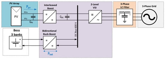
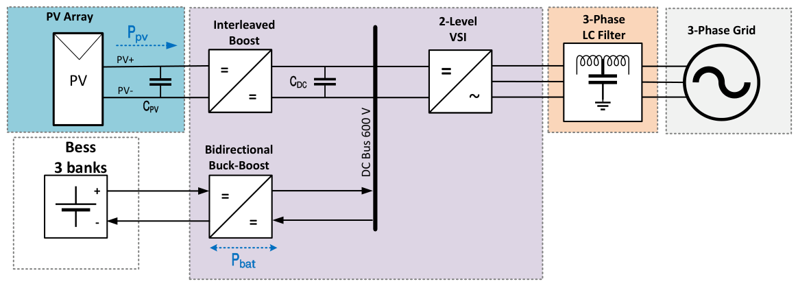
The architecture shown in Figure 1 was implemented, comprising a 91 kWp PV array connected to the grid through three cascaded conversion stages sharing a common 600 V DC bus: three interleaved Boost stages for PV conditioning and MPPT; three bidirectional buck–boost stages managing independent LiFePO₄ banks; and a two-level three-phase voltage source inverter (VSI) with an LC output filter. The 600 V DC bus is the architectural node integrating all subsystems. Its voltage stability conditions the quality of power delivered by the inverter, and this stability depends directly on the ability of the BESS to absorb or supply power during irradiance transients or increases in reactive demand. The main electrical parameters of each stage are consolidated in Table 2.

Figure 1. Functional block diagram of the proposed three-phase photovoltaic system with the BESS and grid connection.

Table 2. Main electrical parameters of each stage of the proposed architecture.

Stage	Main Parameters
PV Array	140 modules; $N_s=10$, $N_p=14$; $V_{mpp,\mathrm{str}}\approx 374 \mathrm{V}$; $I_{mpp,\mathrm{arr}}\approx 250 \mathrm{A}$; $C_{PV}=470 \mathrm{\mu }\mathrm{F}$
Interleaved Boost	3 legs; $f_{sw}=18 \mathrm{k}\mathrm{H}\mathrm{z}$; $D_{nom}\approx 0.38$; $L=1.8 \mathrm{m}\mathrm{H}$
DC Bus	$V_{dc}^{★}=600 \mathrm{V}$; bus capacitance $C_{dc}=12 \mathrm{m}\mathrm{F}$
BESS	3 LiFePO4 banks; $V_{bat}=384 \mathrm{V}$; $I_{max}=100 \mathrm{A}$; $Q_{nom}=100 \mathrm{A}\mathrm{h}$
Bidirectional Buck–Boost	3 legs; $f_{sw}=9 \mathrm{k}\mathrm{H}\mathrm{z}$; $D_{buck}\approx 0.64$; $D_{boost}\approx 0.36$; $L=1.8 \mathrm{m}\mathrm{H}$
Two-Level Three-Phase VSI	$f_{sw}=9 \mathrm{k}\mathrm{H}\mathrm{z}$; d–q control; Volt–VAR support
LC Filter	$L=1.25 \mathrm{m}\mathrm{H}$; $C_f=15 \mathrm{\mu }\mathrm{F}$; $R_f=3.0 \Omega$
Grid	3-phase; $V_{LL}\approx 220 \mathrm{V}$ ($V_{phase}\approx 127 \mathrm{V}$ RMS); $f=60 \mathrm{H}\mathrm{z}$; $P_{max}\approx 91 \mathrm{k}\mathrm{W}$; $Q\le 65 \mathrm{k}\mathrm{V}\mathrm{A}\mathrm{r}$

2.2. PV Array and Interleaved Boost Stage

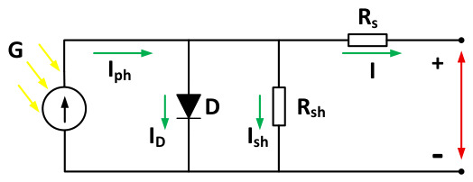
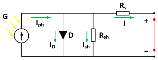
The PV array of Figure 1 is modeled by the single-diode equivalent circuit [24] according to Equation (1):

$$I=I_{ph}-I_0\left[exp\left({\displaystyle \frac{q(V+I{R}_s)}{nkT}}\right)-1\right]-{\displaystyle \frac{V+I{R}_s}{R_{sh}}},$$

(1)

where $I_{ph}$ is the photocurrent, $I_0$ is the reverse saturation current, $R_s$ and $R_{sh}$ are the series and shunt resistances, n is the ideality factor, q is the electron charge, k is the Boltzmann constant, and T is the junction temperature. A three-dimensional look-up table, implemented in PLECS and indexed by voltage, irradiance, and temperature, replaces the iterative numerical solution at each time step, preserving model fidelity without the associated computational cost.

The single-diode equivalent circuit is illustrated in Figure 2, where all variables of Equation (1) are identified.

Figure 2. Single-diode equivalent circuit of the photovoltaic cell. Green arrows indicate current directions ($I_{ph}$, $I_D$, $I_{sh}$, I); yellow arrows indicate the incident solar irradiance (G); the red arrow indicates the output voltage (V).

The PV array consists of 140 Trina Solar TSM-NEG20C.20 panels [25] ($N_s=10$ in series, $N_p=14$ in parallel) at 650 W each, totaling 91 kWp. Table 3 lists the main parameters at STC.

Table 3. Electrical characteristics of the TSM-NEG20C.20 module at STC [25].

Parameter	Value
Maximum power, $P_{max}$	650 W
MPP voltage, $V_{mpp}$	$37.4$ V
MPP current, $I_{mpp}$	$17.38$ A
Open-circuit voltage, $V_{oc}$	$45.1$ V
Short-circuit current, $I_{sc}$	$18.36$ A
Temp. coeff. of $I_{sc}$	0.04%/°C
Temp. coeff. of $V_{oc}$	$-0.24$%/°C
Temp. coeff. of $P_{\max }$	$-0.29$%/°C
NOCT	43(2) °C

At the array MPP, with string voltage $V_{mpp,\mathrm{str}}\approx 374 \mathrm{V}$ (STC nameplate value, $10\times 37.4 \mathrm{V}$, Table 3), the nominal duty cycle of each Boost leg is $D\approx 0.377$. Each leg processes $P_{leg}\approx 30.3 \mathrm{k}\mathrm{W}$. The lower value of 367 V reported for $v_{PV}$ and $V_{mpp}$ in the Case 1 and Case 3 simulation results (Section 4.1 and Section 4.3) is the actual array operating voltage tracked by P&O under the simulated irradiance/temperature profile, which is not required to coincide exactly with the STC nameplate value used here for the nominal sizing calculation. The minimum inductance for continuous conduction mode (CCM) at $f_{sw}=18 \mathrm{k}\mathrm{H}\mathrm{z}$ is $L_{min}\approx 0.05 \mathrm{m}\mathrm{H}$ [26]; the adopted value $L=1.8 \mathrm{m}\mathrm{H}$ ($36\times$ the minimum) substantially reduces the current ripple seen by the array. This margin over $L_{min}$ reflects a deliberate design trade-off rather than an arbitrary choice. Operating close to $L_{min}$ minimizes inductor size, mass, and cost, but leaves little margin against entering discontinuous conduction mode (DCM) during the fast irradiance transients evaluated in Case 1 (Section 4.1), where DCM would distort the P&O power measurement and slow MPP reacquisition. The peak-to-peak current ripple of a Boost stage is $\mathsf{\Delta }{I}_L=D(1-D)V_{in}/\left(L{f}_{sw}\right)$; at the nominal operating point ($D\approx 0.377$, $V_{in}\approx 374 \mathrm{V}$), increasing L from $L_{min}$ to $1.8$ mH reduces $\mathsf{\Delta }{I}_L$ by the same $36\times$ factor, directly lowering the RMS ripple current seen by the PV array and the associated conduction losses and MPPT-induced power oscillation, at the cost of a larger magnetic component and a slower current-loop transient response. Table 4 quantifies this trade-off for three values of L using closed-form relations rather than additional simulation: the ripple formula above, and a current-loop crossover estimate $f_c\approx V_{in}{K}_{p,PV,inner}/\left(2\pi L\right)$ obtained with the same linearized-integrator method used for the DC-bus loop in Section 3.4 (plant $G_p\left(s\right)=V_{in}/\left(Ls\right)$, confirmed PV Boost inner-loop gain $K_p=0.001$ from Table 5). Relative inductor volume is a first-order estimate assuming volume scales linearly with L at fixed peak current, not a physical component measurement. At $L_{min}$, the ripple reaches ≈$39\%$ of the nominal array current $I_{mpp,arr}$ (consistent with the DCM risk flagged above), while the current-loop crossover (≈1.19 kHz) is still comfortably below the 9 kHz Nyquist limit of the 18 kHz sample rate. This confirms that the switching/sampling rate is not the binding constraint across this entire range of L: the $36\times$ increase in L trades a $36\times$ reduction in crossover frequency (from ≈1.19 kHz to ≈33 Hz) and a proportional increase in estimated volume for a $36\times$ reduction in ripple, and the adopted $1.8$ mH was chosen because the resulting 33 Hz bandwidth remains far more than adequate for tracking the second-scale irradiance transients evaluated in this work (Case 1), so the ripple and DCM-margin benefits dominated the selection.

Table 4. Sensitivity of PV Boost ripple, current-loop bandwidth, and relative inductor volume to L (closed-form estimates; see text for the formulas used).

L	$\mathbf{\Delta }{\mathit{I}}_{\mathit{L}}$ (A)	$\mathbf{\Delta }{\mathit{I}}_{\mathit{L}}/{\mathit{I}}_{\mathit{mpp},\mathit{arr}}$	${\mathit{f}}_{\mathit{c}}$ (Hz)	Relative Volume
$L_{min}\approx 0.05 \mathrm{m}\mathrm{H}$	97.6	39%	1190	≈$0.03\times$
$10\times L_{min}=0.5 \mathrm{m}\mathrm{H}$	9.8	3.9%	119	≈$0.28\times$
$36\times L_{min}=1.8 \mathrm{m}\mathrm{H}$ (adopted)	2.7	1.1%	33	$1\times$ (reference)

Table 5. PI gains and output-saturation limits of the seven discrete control loops, extracted directly from the PLECS model (Caso_5Plecs.plecs); all run at $T_s=1/18 \mathrm{k}\mathrm{H}\mathrm{z}$.

Loop	${\mathit{K}}_{\mathit{p}}$	${\mathit{K}}_{\mathit{i}}$	Output Limits
VSI—outer $V_{dc}$ ($\to i_{d,ref}$)	20	200	$\pm 600 \mathrm{A}$
VSI—inner current (→ duty, $d_{Conv}$)	20	200	$\pm 600 \mathrm{A}$
BESS—outer ($V_{dc}\to i_{Lbat,ref}$) ‡	0.0012	0.0008	$\pm 240 \mathrm{A}$
BESS—inner (current $\to d_{bat}$)	0.003	15	$[0.20,0.75]$
PV Boost—outer (voltage $\to i_{ref}$)	0.5	50	$[0,285]$ A
PV Boost—inner (current $\to d_{PV}$)	0.001	0.5	$[0,0.95]$
VSI—Volt–VAR ($\to i_{q,ref}$)	0.1	500	$\pm 390 \mathrm{A}$

Note: loop identity (outer/inner, which stage) follows each loop’s input error source and, for inner loops, the destination Goto tag (dPv, dBat, or dConv) in the PLECS Connection table. No dedicated inner PI loop exists for $i_q$; the C-Script instead applies a first-order smoothing filter (ICOMP_ALPHA_UP/DOWN) to the reactive current command before it reaches the modulator. ^‡ The Sum-block inputs feeding both outer loops show that both the VSI and the BESS outer loops compare the same $V_{dc}$ measurement against the same $600 \mathrm{V}$ reference: a coordinated, dual-actuator DC-bus regulation scheme, not two independently tuned voltage loops. The VSI loop’s proportional and integral gains are, respectively, ∼$1.7\times {10}^4$ and ∼$2.5\times {10}^5$ times larger than the BESS loop’s, so the VSI loop dominates the fast bus dynamics while the BESS loop acts as a slow trim term (consistent with the $0.05i_{Lbat,\Sigma }[k-1]$ damping term described in Section 3.2).

The variables D, $L_{min}$, and $P_{leg}$ are identified in the PV Boost control structure detailed in Section 3.1. A 470 μF capacitor on the PV bus, combined with the array’s incremental output impedance, sets a corner frequency of ≈$250 \mathrm{H}\mathrm{z}$ for the PV-side voltage ripple; keeping this corner well above the 10 Hz P&O sampling rate ($1/100 \mathrm{m}\mathrm{s}$) prevents the switching-frequency ripple from being aliased into the MPPT power measurement, while remaining well below $f_{sw}$ so that the capacitor does not need to attenuate switching harmonics directly (that role is left to the interleaving of the three legs) [27]. The three legs operate with 120°-shifted PWM carriers, partially canceling individual ripples without increasing the switching frequency per device.

2.3. LC Output Filter

The VSI is current-controlled, as detailed in Section 3.3; the LC topology, rather than a simple L filter, was chosen at the output stage because its $-40 \mathrm{dB}/\mathrm{dec}$ second-order roll-off attenuates PWM switching harmonics more efficiently per millihenry of series inductance, for a given ripple and total component volume, independently of whether the converter is voltage- or current-controlled [28,29]. With $S_{nom}\approx 91 \mathrm{k}\mathrm{V}\mathrm{A}$ and $V_{LL}\approx 220 \mathrm{V}$, the nominal RMS line current is $I_L=S_{nom}/\left(\sqrt{3}{V}_{LL}\right)\approx 238.8 \mathrm{A}$ (peak $\approx 337.7 \mathrm{A}$). This value ($V_{phase}\approx 127 \mathrm{V}$ RMS, ≈$180 \mathrm{V}$ peak) is the correct design voltage, independently corroborated by four sources in the PLECS/HIL model: the grid-source amplitude block, the HIL three-phase source parameter, direct measurement of the Vabc signal at the PCC, and algebraic reconstruction of $v_d,v_q$ from the simulated P, Q, $i_d$, $i_q$ of Case 3. Limiting the peak current ripple to 10% of this peak at $f_{sw}=9 \mathrm{kHz}$, the minimum required inductance is $L_{min}=V_{dc}/\left(8f_{sw}\mathsf{\Delta }{I}_{L,max}\right)\approx 0.25 \mathrm{m}\mathrm{H}$; the adopted value $L=1.25 \mathrm{m}\mathrm{H}$ ($5\times$ the minimum) reduces the actual ripple to ≈$2.0\%$ of the peak line current. With the adopted capacitor $C_f=15 \mathrm{\mu }\mathrm{F}$, the resulting voltage ripple is ≈$3.1 \mathrm{V}$, or ≈$1.7\%$ of the (corrected) phase peak voltage, comfortably within typical grid-interface tolerances, yielding a resonance frequency

$$f_{res}={\displaystyle \frac{1}{2\pi \sqrt{L{C}_f}}}\approx 1.16 \mathrm{k}\mathrm{H}\mathrm{z},$$

(2)

satisfying $f_{grid}<f_{res}<f_{sw}/2$ (60 Hz < 1.16 kHz < 4.5 kHz). Passive damping is provided by $R_f=3.0 \Omega$ in series with $C_f$, sized as one-third of the capacitor impedance at resonance [29].

2.4. Battery Energy Storage System

Each of the three independent battery banks consists of 30 series LiFePO₄ modules (Power Queen, 12.8 V/100 Ah), resulting in $V_{bat}=384 \mathrm{V}$, a maximum current of 100 A, a maximum power of $38.4$ kW, and an energy capacity of $38.4$ kWh (numerically equal to the power rating at the 1C discharge rate). Three banks in parallel therefore provide a total power capacity of $115.2$ kW and a total energy capacity of $115.2$ kWh.

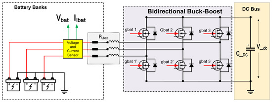
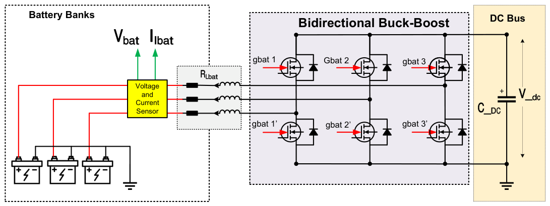
Each bank is interfaced to the 600 V DC bus through a bidirectional buck–boost leg (Figure 3), with nominal duty cycles $D_{buck}\approx 0.64$ and $D_{boost}\approx 0.36$. Three parallel legs at 9 kHz require $L_{min}=0.26 \mathrm{m}\mathrm{H}$; the same 1.8 mH inductor from the Boost stage is adopted for component standardization. In PLECS, each bank is represented by a reduced-order L–C equivalent circuit ($L=1.8 \mathrm{m}\mathrm{H}$, $C=25$ F) that reproduces the dynamic voltage variation within the simulation window [30]. The energy-equivalent capacitor for the full bank would be approximately 1875 F (i.e., C stores only ≈$1/75$ of the energy an equivalent full-scale capacitor would). This simplification is adequate for the transient behavior analyzed here (voltage response of the DC-bus and current-loop controllers over intervals of seconds), but it is not intended to reproduce the long-horizon SOC trajectory of a real 100 Ah bank: the SOC integrator of Equation (7) is driven directly by the measured bank current rather than by the reduced capacitor voltage, so the coulomb-counted SOC and the curtailment trigger remain physically scaled to the real 100 Ah capacity even though the L–C circuit’s own energy content does not. Extending the model to multi-hour or multi-day charge/discharge cycles would require a full-capacity electrochemical or equivalent-circuit battery model rather than this reduced-order representation. The parameter $R_{Lbat}$ in Figure 3 represents the series resistance of the buck–boost leg inductor.

Figure 3. Bidirectional buck–boost interface between the three BESS banks and the 600 V DC bus, as implemented in PLECS. Green arrows indicate the bank voltage ($V_{bat}$) and current ($I_{bat}$) measurement points; black arrows indicate the DC-bus voltage.

The inverter reactive power capacity as a function of active power is $Q_{max}\left(P\right)=\sqrt{S_{nom}^2-P^2}$, with $S_{nom}\approx 91 \mathrm{k}\mathrm{V}\mathrm{A}$. For $P=65 \mathrm{k}\mathrm{W}$, $Q_{max}\approx 64.3 \mathrm{k}\mathrm{V}\mathrm{A}\mathrm{r}$, evidencing the reactive margin gained whenever active power is reduced, the same mechanism that widens $Q_{disp}$ as PV surplus is redirected to BESS charging during the overvoltage segment of Case 4 (Section 4.4). This apparent-power limit is not the only physical constraint on the achievable $(i_d,i_q)$ pair. Two additional limits bound the operating region. First, the line current itself is bounded: at $S_{nom}$, the nominal RMS line current is $I_L=S_{nom}/\left(\sqrt{3}{V}_{LL}\right)\approx 238.8 \mathrm{A}$ (peak $\approx 337.7 \mathrm{A}$, matching the $I_{d,max}=335 \mathrm{A}$ saturation limit configured in the PLECS current-loop controllers), the same current level used to size the LC filter in Section 2.3; any $(i_d,i_q)$ combination whose vector magnitude exceeds this current stresses the filter inductor and the semiconductors beyond their design point even when $S\le S_{nom}$ is nominally satisfied by the outer-loop reference. Second, the modulation index is bounded by the DC-bus voltage: with $V_{dc}=600 \mathrm{V}$ and space-vector modulation, the maximum linear-region phase peak voltage is $V_{dc}/\sqrt{3}\approx 346.4 \mathrm{V}$; at the nominal grid phase peak voltage of ≈$180 \mathrm{V}$, the modulation index is $m_a\approx 0.52$, leaving a comfortable margin before saturation even under the overvoltage excursions evaluated in Cases 4–5. $Q_{max}\left(P\right)$ therefore represents a necessary but not sufficient condition for feasible operation; a combined current-magnitude and modulation-index limiter, in addition to the $S\le S_{nom}$ check, is recommended for scenarios approaching the current boundary in particular, since it is markedly closer to the values reached in Cases 3–5 (Section 4) than the modulation-index boundary is. In the C-Script source, the supervisory block computes $I_{q,req}=\mathrm{sat}(\left|Q_{ref}\right|/K_{IQ\_TO\_KVAR},0,I_{MAX\_INV})$ and $I_{d,allowed}=\sqrt{I_{MAX\_INV}^2-I_{q,req}^2}$, i.e., a genuine vector-magnitude circle limit on $\sqrt{i_d^2+i_q^2}\le I_{MAX\_INV}=335 \mathrm{A}$, not a check on $i_d$ in isolation. The resulting margin $I_{MAX\_INV}-I_{d,allowed}$ directly feeds the $\mathsf{\Delta }{I}_{d,max}$ mechanism already described in Section 3.4, i.e., $I_{d,max}$ is dynamically reduced whenever the reactive demand alone would otherwise push the current vector outside the 335 A circle. $Q_{max}\left(P\right)$ constrains apparent power, while this separate current-circle mechanism constrains the current vector magnitude directly, and both act simultaneously on the achievable $(i_d,i_q)$ operating region in Cases 3–5.

3. Proposed Control Strategy

3.1. PV Stage: Cascade Control and MPPT

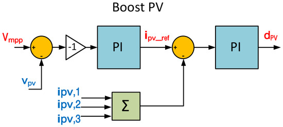
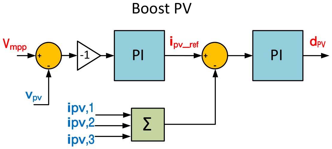
An interleaved Boost stage was implemented to operate under a two-loop cascade controller (Figure 4). The outer voltage loop tracks the MPPT reference $V_{mpp}$ and generates $i_{PV,ref}$ via a PI regulator. The inner loop converts this reference into the duty cycle $d_{PV}$ applied to the three legs, with 120°-shifted PWM carriers.

Figure 4. Voltage–current cascade structure of the interleaved PV Boost stage.

The Perturb and Observe (P&O) algorithm, a maximum-power-point-tracking method that periodically increments or decrements the voltage reference and observes the sign of the resulting power variation, was implemented in the C-Script block with a period of 100 ms (1800 cycles). A step-direction memory variant was adopted to reduce oscillation around the MPP under constant irradiance while preserving tracking speed under transient variations. P&O was selected over model-based or soft-computing alternatives (e.g., incremental conductance, fuzzy-logic, or particle-swarm MPPT) because it requires only the voltage and current already measured for the outer control loop; it adds no extra sensing hardware; and its known drawback, steady-state oscillation around the MPP and transient mistracking under fast-changing irradiance, is directly mitigated here by the step-direction memory variant together with the ≈$250 \mathrm{H}\mathrm{z}$ PV-bus ripple corner discussed in Section 2.2. The irradiance profiles evaluated in this work (Case 1) are ramps on the order of seconds, well within the P&O tracking bandwidth at a 100 ms update period; faster-changing profiles, such as fast-moving cloud edges, would favor a model-based method and are identified as future work.

3.2. BESS: DC-Bus Regulation

The BESS converters were implemented as the primary active regulators of the DC bus. The power balance at the bus is given by

$$C_{dc}{V}_{dc}{\displaystyle \frac{d{V}_{dc}}{dt}}=p_{PV}+p_{BESS}-p_{inv}-p_{losses},$$

(3)

where $C_{dc}$ is the bus capacitance, $V_{dc}$ its voltage, $p_{PV}$ the power injected by the PV array, $p_{BESS}$ the power supplied or absorbed by the storage system, $p_{inv}$ the power transferred to the inverter, and $p_{losses}$ the losses in passive elements. This equation shows that any imbalance between generation and load manifests directly as a deviation in $V_{dc}$.

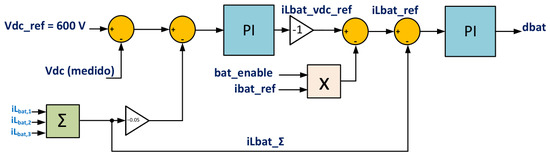
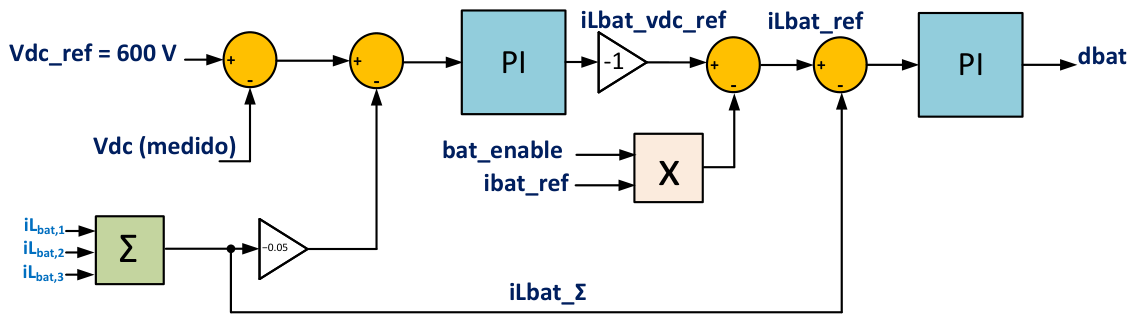
A discrete cascade controller was implemented (Figure 5): the outer voltage loop compares $V_{dc}$ with the 600 V reference, adds a partial derivative damping term based on the total bank current $i_{Lbat,\Sigma }$, and generates $i_{Lbat,ref}^{★}$; the inner current loop produces the duty cycle $d_{bat}$ for three 120°-interleaved buck–boost legs. The term $0.05i_{Lbat,\Sigma }[k-1]$ improves the transient response without altering the steady-state operating point. The voltage reference $V_{dc}^{★}=600 \mathrm{V}$ is the outer-loop setpoint, as indicated in Figure 5.

Figure 5. Discrete voltage–current cascade control of the BESS buck–boost stage.

3.3. Grid-Connected Inverter: SRF Vector Control and Volt–VAR

The VSI is controlled in the synchronous reference frame (SRF). The SRF-PLL estimates $\widehat{\theta }$ by driving the q-axis voltage to zero via the Park Transform, applied to the instantaneous three-phase quantities:

$$\left[\begin{array}{c}{v}_d\\ v_q\end{array}\right]={\displaystyle \frac{2}{3}}\left[\begin{array}{ccc}cos\left(\widehat{\theta }\right)& cos(\widehat{\theta }-{\displaystyle \frac{2\pi }{3}})& cos(\widehat{\theta }+{\displaystyle \frac{2\pi }{3}})\\ -sin\left(\widehat{\theta }\right)& -sin(\widehat{\theta }-{\displaystyle \frac{2\pi }{3}})& -sin(\widehat{\theta }+{\displaystyle \frac{2\pi }{3}})\end{array}\right]\left[\begin{array}{c}{v}_a\\ v_b\\ v_c\end{array}\right],$$

(4)

the same transform applied to the line currents to obtain $i_d,i_q$. Under synchronism, $v_q\approx 0$ and the active and reactive powers decouple:

$$P={\displaystyle \frac{3}{2}}\left(v_d{i}_d+v_q{i}_q\right)\approx {\displaystyle \frac{3}{2}}{v}_d{i}_d,Q={\displaystyle \frac{3}{2}}\left(v_d{i}_q-v_q{i}_d\right)\approx {\displaystyle \frac{3}{2}}{v}_d{i}_q,$$

(5)

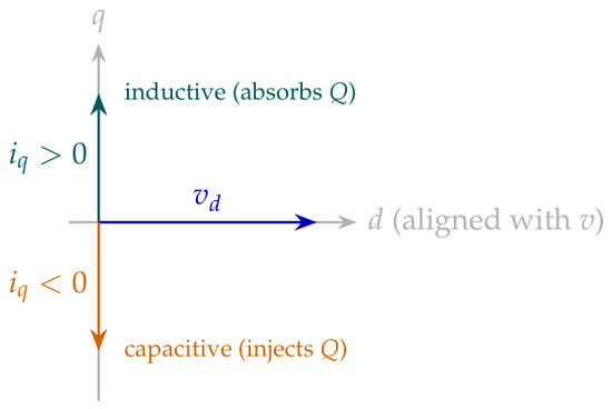
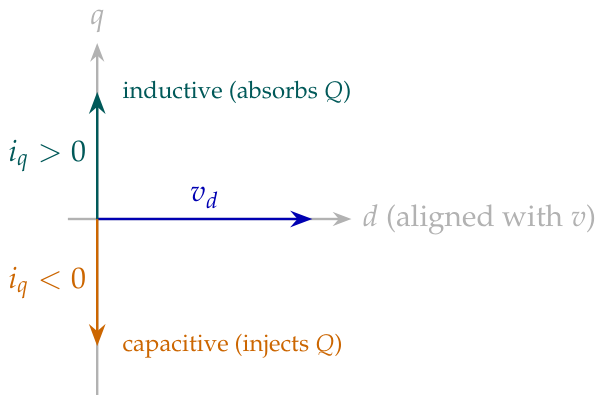
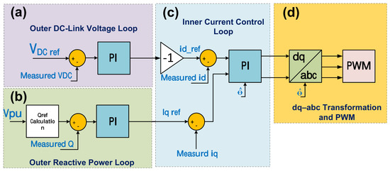
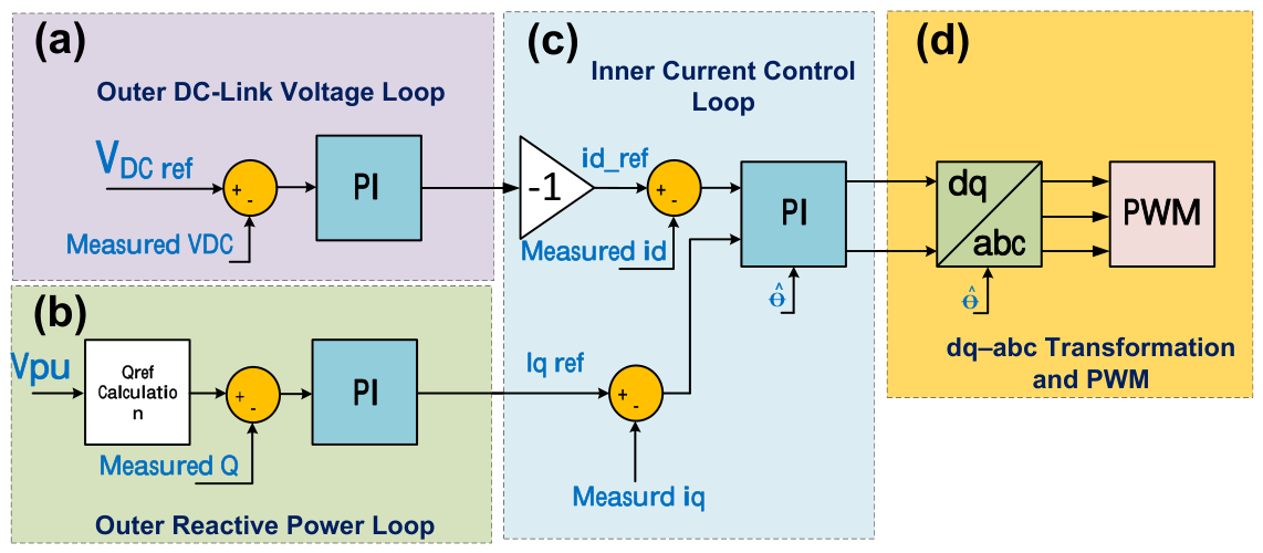
with the $2/3$ forward-transform and $3/2$ power coefficients corresponding to the amplitude-invariant Clarke/Park convention (i.e., $v_a,v_b,v_c$ are instantaneous peak-scaled quantities, and $v_d$, $i_d$, $i_q$ are consequently peak, not RMS, quantities). Under this convention, d-axis current aligned with the grid voltage vector produces positive active power, and a negative $i_q$ corresponds to leading (capacitive) reactive current injection, while a positive $i_q$ corresponds to lagging (inductive) absorption, as illustrated by the phasor diagram of Figure 6. The outer DC-bus voltage loop defines $i_{d,ref}$; the Volt–VAR loop defines $i_{q,ref}$; inner PI current controllers track both references (Figure 7).

Figure 6. Sign convention for the reactive current $i_q$ relative to the grid voltage vector $v_d$, consistent with $Q\approx \frac{3}{2}{v}_d{i}_q$ under the amplitude-invariant Park transform used throughout this work.

Figure 7. Block diagram of the VSI control in the synchronous reference frame: (a) outer DC-bus voltage loop; (b) outer reactive power loop; (c) inner current control loop; (d) $dq$–$abc$ transformation and PWM modulator. The angle $\widehat{\theta }$ is supplied by the SRF-PLL.

The Volt–VAR function applies no reactive action within the dead band $[0.90,1.10]$ pu: below 0.90 pu, it injects capacitive reactive power (negative $i_q$); above 1.10 pu, it absorbs inductive reactive power (positive $i_q$); the reactive reference is bounded at every instant by $Q_{max}\left(P\right)$, preventing inverter overload. This $\pm 10\%$ band is wider than the default $\pm 3\%$ dead band of IEEE 1547-2018 [23] Category B ($V_2$–$V_3=0.97$–$1.03$ pu) and wider than the $0.85$–$1.10$ pu normal-operation range shared by EN 50549-1 [31] and IEC 61727 [32] and, for this 220 V-line system (Section 2.3), by ANEEL PRODIST Module 8 [33] (202–231 V, i.e., $0.918$–$1.050$ pu). It was adopted deliberately so the reactive channel stays inactive through Case 1’s moderate excursions (0.93–1.07 pu, within IEEE 1547-2018’s own dead band) while engaging the severe low-SCR events of Cases 2–5, which exceed the normal-service range of all four standards and are intended as ride-through stress tests rather than routine regulation; IEEE 1547-2018’s tighter $\pm 3\%$ curve is the recommended starting point for a deployment-oriented retuning. Case 4 (Section 4.4) sustains a 0.80 pu undervoltage segment for 4.5 s followed by a 1.20 pu overvoltage segment for 3 s, each exceeding the continuous operating range defined by most interconnection standards and therefore explicitly framed here as ride-through tests, verifying that the reactive control loop remains stable and correctly signed under abnormal, non-momentary events, rather than as sustained normal-operation conditions. Case 5 (Section 4.5) evaluates a comparable sustained overvoltage step to ≈$1.20$ pu, but with the BESS already saturated at $SOC\approx 0.97$ rather than the 50% headroom available in Case 4, explicitly testing the limit at which PV curtailment, rather than reactive support or BESS charging, must protect the DC bus.

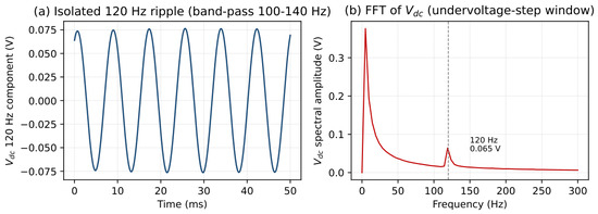
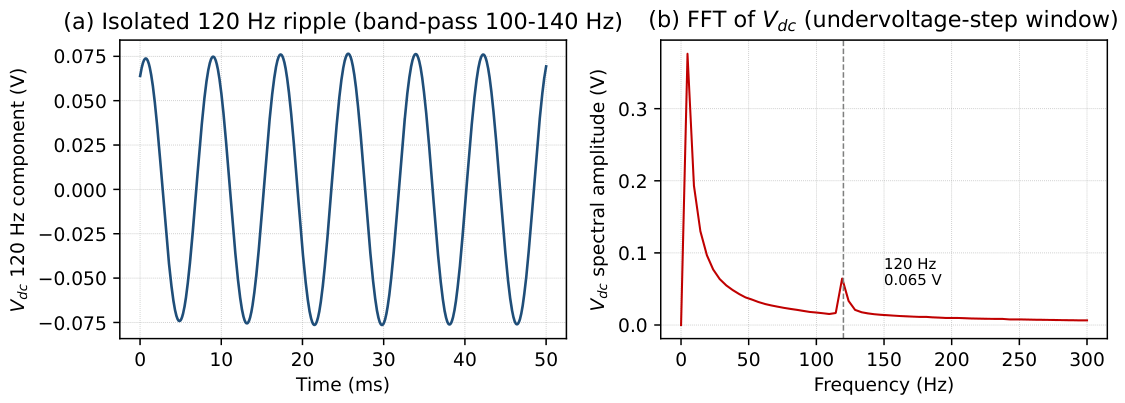
A known limitation of the SRF-PLL, well documented in recent stability studies of inverter-based resources under weak-grid and unbalanced conditions [5,6], is its performance under unbalanced grid conditions: a 2% negative-sequence component rotates at $-60 \mathrm{H}\mathrm{z}$ in the stationary frame, so relative to the SRF rotating at $+60 \mathrm{H}\mathrm{z}$, it appears as a 120 Hz oscillation that the SRF-PLL cannot attenuate, leaking into the estimated angle $\widehat{\theta }$ and producing a 120 Hz ripple on $V_{dc}$. This was verified directly by injecting a 2% negative-sequence component into the grid-side source (reordering the phase sequence of the existing positive-sequence signal to a-c-b, scaling by 0.02, and summing it back before the point of common coupling) and re-running the Case 1 disturbance profile. An initial estimate using a 500 Hz low-pass filter on $V_{dc}$ overstated the ripple because it also captured slower, unrelated settling dynamics from the grid-voltage and irradiance steps; isolating the ripple with a narrow 100–140 Hz band-pass filter, its true peak-to-peak amplitude is ≈0.13–0.18 V across the three tested disturbance windows (undervoltage step, overvoltage step, and post-irradiance step), essentially independent of the operating current level within this range. Figure 8 shows the isolated time-domain ripple and its FFT, confirming the peak at exactly 120 Hz (ruling out switching-frequency leakage) and two orders of magnitude smaller than a simplified analytical upper bound of 8–15 V, which does not capture the attenuating effect of the large bus capacitance $C_{dc}=12 \mathrm{m}\mathrm{F}$ on a 2% negative-sequence imbalance (Section 3.4). All five main scenarios (Section 4.1, Section 4.2, Section 4.3, Section 4.4 and Section 4.5) otherwise assume a balanced, undistorted grid; a DSOGI-PLL or dual-sequence extractor, which would eliminate this sensitivity entirely, is reserved for future work.

Figure 8. $V_{dc}$ ripple under a 2% negative-sequence grid imbalance: (a) time-domain ripple isolated with a 100–140 Hz band-pass filter; (b) FFT spectrum of $V_{dc}$, confirming a distinct peak at 120 Hz separated from the larger low-frequency content associated with the Case 1 disturbance transients.

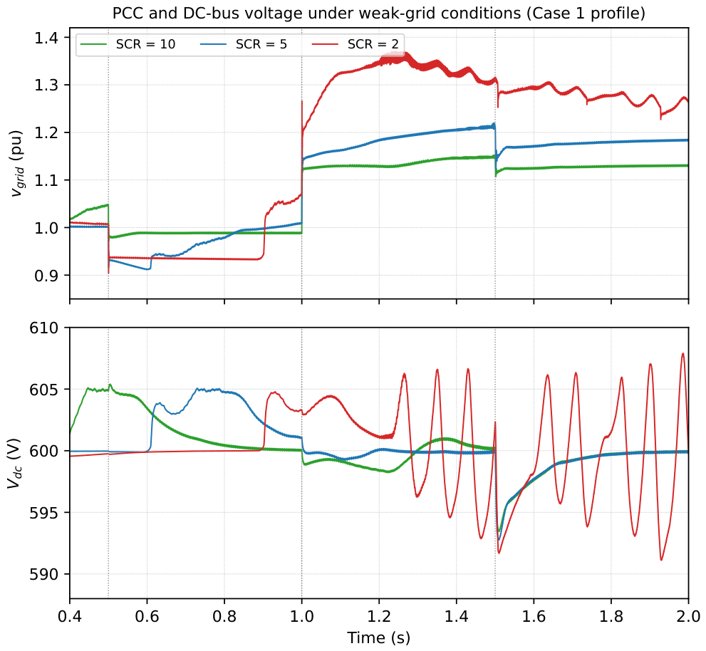
Additionally, all five scenarios of Section 4.1, Section 4.2, Section 4.3, Section 4.4 and Section 4.5 represent the grid as an ideal voltage source with a prescribed voltage profile. Under an ideal source, reactive current injection cannot, by construction, change the voltage at the point of common coupling (PCC), so those results demonstrate correct commanded-current tracking and DC-bus/BESS stability but not PCC voltage support on a weak feeder. To address this directly, a Thévenin equivalent $Z_{th}=R_{th}+j{X}_{th}$ (assuming $X/R=1$, representative of a low-voltage rural feeder where resistance is not negligible relative to reactance) was inserted between the LC-filter output and the ideal source, sized from the declared short-circuit ratio, $Z_{th}=V_{LL}^2/(SCR·S_{nom})$, for $SCR\in \{10,5,2\}$ ($S_{nom}\approx 91 \mathrm{k}\mathrm{V}\mathrm{A}$, $V_{LL}=220 \mathrm{V}$); $L_{th}=0.10 \mathrm{m}\mathrm{H}$/$R_{th}=0.038 \Omega$ for $SCR=10$; $L_{th}=0.20 \mathrm{m}\mathrm{H}$/$R_{th}=0.075 \Omega$ for $SCR=5$; and $L_{th}=0.50 \mathrm{m}\mathrm{H}$/$R_{th}=0.188 \Omega$ for $SCR=2$. The Case 1 disturbance profile (Section 4.1) was re-run once per SCR value with the source held at nominal voltage, so that any PCC voltage deviation would be attributable only to the inverter’s own current flowing through $Z_{th}$ and not to an externally imposed source-side step.

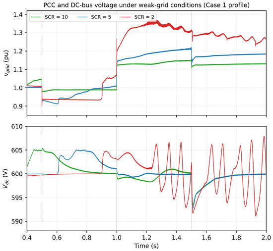
Figure 9 shows the resulting $v_{grid}$ (PCC, per unit) and $V_{dc}$ traces. Following the irradiance step at $t=1.5$ s (the cleanest window, isolating the weak-grid effect from the source-side voltage steps at $t=0.5$ s and $t=1.0$ s), the PCC voltage settles at ≈1.13 pu for $SCR=10$, ≈1.18 pu for $SCR=5$, and ≈1.27 pu for $SCR=2$, a monotonic, roughly threefold increase in PCC voltage deviation as the grid weakens from $SCR=10$ to $SCR=2$ for the identical disturbance, directly demonstrating the degraded voltage-regulation authority expected on low-SCR feeders. During the source-side voltage steps ($t=0.5$–$1.5$ s), the ordering across SCR values is less clean, since the closed-loop Volt–VAR response to the imposed step interacts with $Z_{th}$ rather than reflecting the weak-grid sensitivity in isolation. A further finding, verified at 50 kHz temporal resolution (well above the 18 kHz switching frequency, ruling out aliasing of PWM ripple), to confirm it is a genuine low-frequency phenomenon and not a sampling artifact, is that at $SCR=2$, $V_{dc}$ develops a sustained, slowly growing oscillation with a period of ≈80–115 ms (≈9–12 Hz) and peak-to-peak amplitude reaching ≈17 V by the end of the window, which is absent at $SCR=5$ and $SCR=10$ (which both settle smoothly to 600 V). This indicates that at $SCR=2$, the coordinated VSI/BESS DC-bus regulation (Section 3.4) approaches its stability margin under the added grid impedance, a genuine weak-grid interaction effect rather than a modeling artifact, and is reported here as a limitation requiring further controller re-tuning or feed-forward compensation for deployment on very weak feeders ($SCR\lesssim 2$).

Figure 9. PCC voltage $v_{grid}$ (pu) and DC-bus voltage $V_{dc}$ (V) under the Case 1 disturbance profile, repeated for three short-circuit ratios ($SCR=10,5,2$) with a Thévenin equivalent grid impedance. Vertical dotted lines mark the grid-voltage steps ($t=0.5$, $1.0$ s) and the irradiance step ($t=1.5$ s).

3.4. Controller Design and Tuning

All converter stages (PV Boost, BESS buck–boost, and VSI) are regulated by discrete cascade PI structures: an outer loop that tracks the stage’s energy/voltage reference and an inner loop that tracks the resulting current reference. All seven PI controllers execute at the same discrete sample time, $T_s=1/f_{sw,PV}=1/18 \mathrm{k}\mathrm{H}\mathrm{z}\approx 55.6 \mathrm{\mu }\mathrm{s}$, independent of each stage’s own PWM carrier frequency (18 kHz for the PV Boost and BESS legs, 9 kHz for the VSI, per Table 2); the control update rate and the switching/carrier frequency are therefore distinct design parameters in this implementation. Table 5 lists the proportional and integral gains and output-saturation limits of each loop, extracted directly from the PLECS model. State-space/pole-placement and LQR alternatives were considered and discarded in favor of this discrete PI cascade because it is directly compatible with the block-diagram implementation adopted in PLECS, its tuning is more direct, and it is sufficient for the DC-bus and current-regulation objectives pursued here. The BESS outer voltage loop adds a one-sample-delayed proportional damping term on the total bank current, $0.05i_{Lbat,\Sigma }[k-1]$ (Section 3.2), which improves transient response without changing the steady-state operating point. The Volt–VAR loop tracks the reactive power error $e_Q\left[k\right]=Q_{ref}\left[k\right]-Q_{out}\left[k\right]$ directly with a discrete PI, followed by a saturation block that bounds $i_{q,ref}$ to the values admissible by the converter; anti-windup is implemented by clamping each PI integrator whenever the corresponding duty cycle or current reference saturates, preventing integrator wind-up when the requested reactive power exceeds the instantaneous inverter capacity. Discretization uses the trapezoidal (Tustin) integration method for every loop, and anti-windup is implemented predominantly by back-calculation, with output clamping applied to the BESS inner current loop.

The dominant DC-bus loop (VSI outer $V_{dc}\to i_{d,ref}$) was linearized around the $V_{dc}^{★}=600 \mathrm{V}$ operating point using the power-balance relation of Equation (3). With the inverter’s active-power injection $p_{inv}=\frac{3}{2}{v}_d{i}_d$ (amplitude-invariant convention, grid-voltage-oriented frame, and peak phase voltage) and treating it as a slow disturbance, the small-signal plant is a pure integrator,

$$G_p\left(s\right)={\displaystyle \frac{\mathsf{\Delta }{V}_{dc}\left(s\right)}{\mathsf{\Delta }{i}_d\left(s\right)}}={\displaystyle \frac{3v_d}{2C_{dc}{V}_{dc}^{★}s}}\approx {\displaystyle \frac{37.5}{s}},$$

(6)

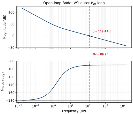
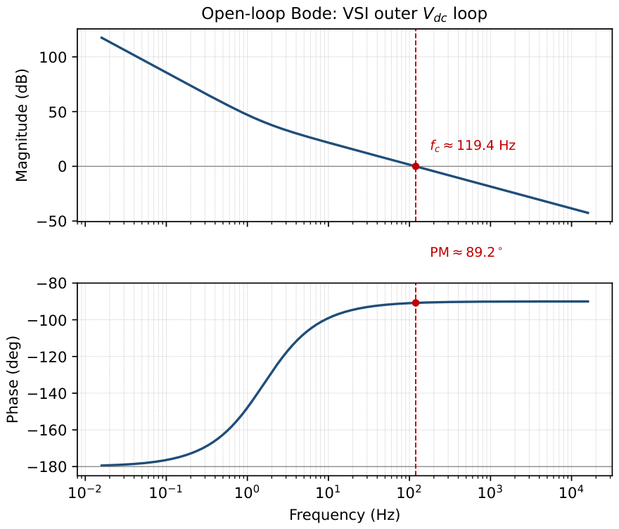
using the confirmed bus capacitance $C_{dc}=12 \mathrm{m}\mathrm{F}$ (three capacitors, $10 \mathrm{m}\mathrm{F}+1 \mathrm{m}\mathrm{F}+1 \mathrm{m}\mathrm{F}$, tied to the shared VDC+ net across the three inverter legs in Caso_5Plecs.plecs). With the continuous-time approximation of the discrete PI ($K_p=20$, $K_i=200$, valid since the resulting crossover is far below the $T_s=1/18 \mathrm{k}\mathrm{H}\mathrm{z}$ Nyquist frequency of 9 kHz), the open-loop transfer function $L\left(s\right)=(K_p+K_i/s)G_p\left(s\right)$ has a gain crossover at $f_c\approx 119 \mathrm{H}\mathrm{z}$ with a phase margin of $\mathrm{PM}\approx {89}^{\circ }$; no phase crossover occurs below the Nyquist limit, so the gain margin is effectively unbounded within the loop’s valid bandwidth. Figure 10 shows the corresponding Bode diagram. The large phase margin reflects the deliberately conservative, well-damped tuning already used in the PLECS model rather than an artifact of the linearization, characterizing the small-signal stability margin of the system’s most critical loop.

Figure 10. Open-loop Bode diagram of the dominant DC-bus voltage loop (VSI outer $V_{dc}\to i_{d,ref}$), linearized per Equation (6): gain crossover $f_c\approx 119 \mathrm{H}\mathrm{z}$, phase margin $\approx {89}^{\circ }$.

3.5. C-Script Supervisory Block

A C-Script block running at 18 kHz was implemented to integrate three supervisory functions:

(i)

P&O MPPT producing $V_{mpp}$ every 1800 cycles.

(ii)

Per-bank SOC estimation via coulomb counting, according to

$$SO{C}_k[n+1]=SO{C}_k\left[n\right]+i_{Lbat,k}\left[n\right]·K_{SOC},K_{SOC}={\displaystyle \frac{T_s}{C_{bat}·3600}};$$

(7)

with the control sample time $T_s=1/18 \mathrm{k}\mathrm{H}\mathrm{z}$ and the nominal bank capacity $C_{bat}=100 \mathrm{A}\mathrm{h}$, Equation (7) yields $K_{SOC}\approx 1.54\times {10}^{-10}$. In the C-Script implementation, however, the bank-capacity macro is set to #define CAP_BANK_AH 1.0f (i.e., 1 Ah) rather than the physical 100 Ah value, so the coulomb counter used to produce the SOC traces in Section 4.4 and Section 4.5 advances $100\times$ faster than the real battery bank would. For a 27 A charging current, this yields the simulated rate of $27/(1\times 3600)\approx 7.5\times {10}^{-3}$ pu/s reported in Section 4.4, a factor of ≈$100\times$ faster than the physically correct bank, which would charge at ≈$7.5\times {10}^{-5}$ pu/s, i.e., 100 times slower. The authors have elected not to re-run Cases 4–5 and instead report the SOC results with this accelerated internal time base made explicit: every SOC excursion and rate quoted for Cases 4–5 should be read as occurring on a time scale $100\times$ faster than a physical 100 Ah bank would exhibit under the same current profile, with the qualitative behavior (monotonic charging, curtailment trigger at $SOC=1.0$, per-bank balance) unaffected by the scaling.

(iii)

Curtailment logic that limits the PV active power reference to the available grid export capacity whenever any bank reaches $SOC=1.0$, preventing DC-bus overvoltage while keeping the reactive channel fully operational.

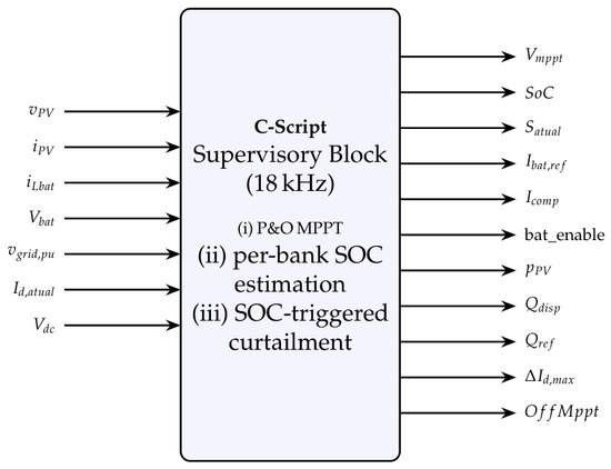
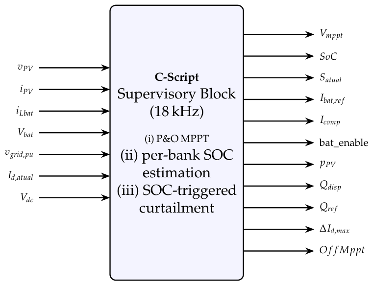
The input–output interface of the C-Script block is illustrated in Figure 11. Inputs comprise the PV voltage $v_{PV}$, PV current $i_{PV}$, battery current $i_{Lbat}$, battery voltage $V_{bat}$, grid voltage in per unit $v_{grid,pu}$, measured active current $I_{d,atual}$, and DC-bus voltage $V_{dc}$. The block exposes 11 outputs to the local control loops: $V_{mppt}$, $SoC$, $S_{atual}$ (estimated apparent power), $I_{bat,ref}$, $I_{comp}$, $bat\_enable$, $p_{PV}$, $Q_{disp}$, $Q_{ref}$, $\mathsf{\Delta }{I}_{d,max}$, and $OffMppt$.

Figure 11. Input–output interface of the C-Script supervisory block, as implemented in PLECS (redrawn natively for clarity and consistent labeling; see Section 3.5 for the full input/output list).

4. Results and Discussion

All five scenarios share the following base conditions: grid frequency 60 Hz, $V_{dc}^{★}=600 \mathrm{V}$, array temperature 25 °C, and Volt–VAR enabled. An initial transient settling interval is excluded from each analysis window. Table 6 summarizes the main differences between scenarios before the individual subsections.

Table 6. Characterization of the five simulation scenarios.

Case	Irradiance (pu)	Grid Voltage (pu)	BESS	Curt.	Main Feature
1	1.00 → 0.50	0.93–1.07 (dead band)	Inactive	No	DC-bus regulation under irradiance step
2	0	0.80 → 1.20	Inactive †	No	Pure reactive compensator without PV
3	1.00	0.85 → 1.15	Inactive	No	Full PV with grid voltage steps
4	1.00	0.80 → 1.20 ‡	50% → Charging (both segments)	No	Bidirectional 9 s test; current-vector limiter redirects PV surplus to BESS in both directions
5	1.00	1.00 → 1.20 (sustained)	SOC ≈ 0.97 (saturated)	Yes	Overvoltage ride-through with curtailment

^† With PV and BESS both inactive, DC-bus regulation duty transfers to the VSI, which imports a small active current from the grid to cover filter and switching losses (see Section 4.2). ^‡ Case 4 additionally holds a 1 s dead interval at a nominal voltage between the two disturbance segments (see Section 4.4).

The scenarios progress from a reactive-free reference (Case 1), through isolated evaluation of the reactive channel (Cases 2–3), to coordinated multi-subsystem operation (Cases 4–5).

4.1. Case 1: Moderate Grid Voltage Variations with Irradiance Step

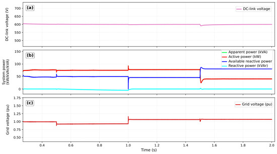
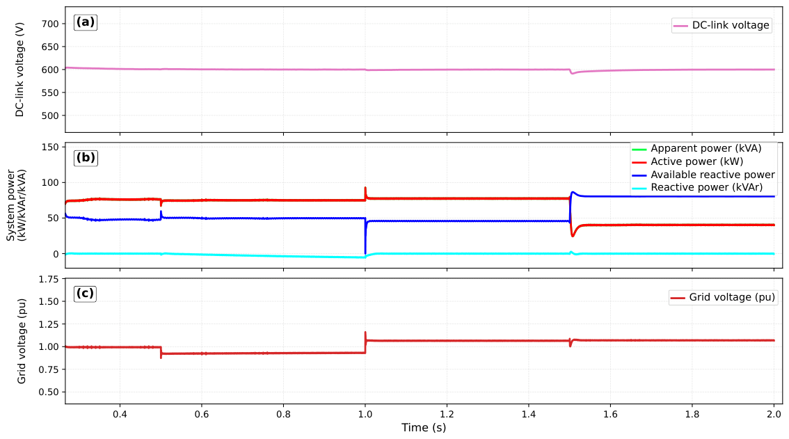
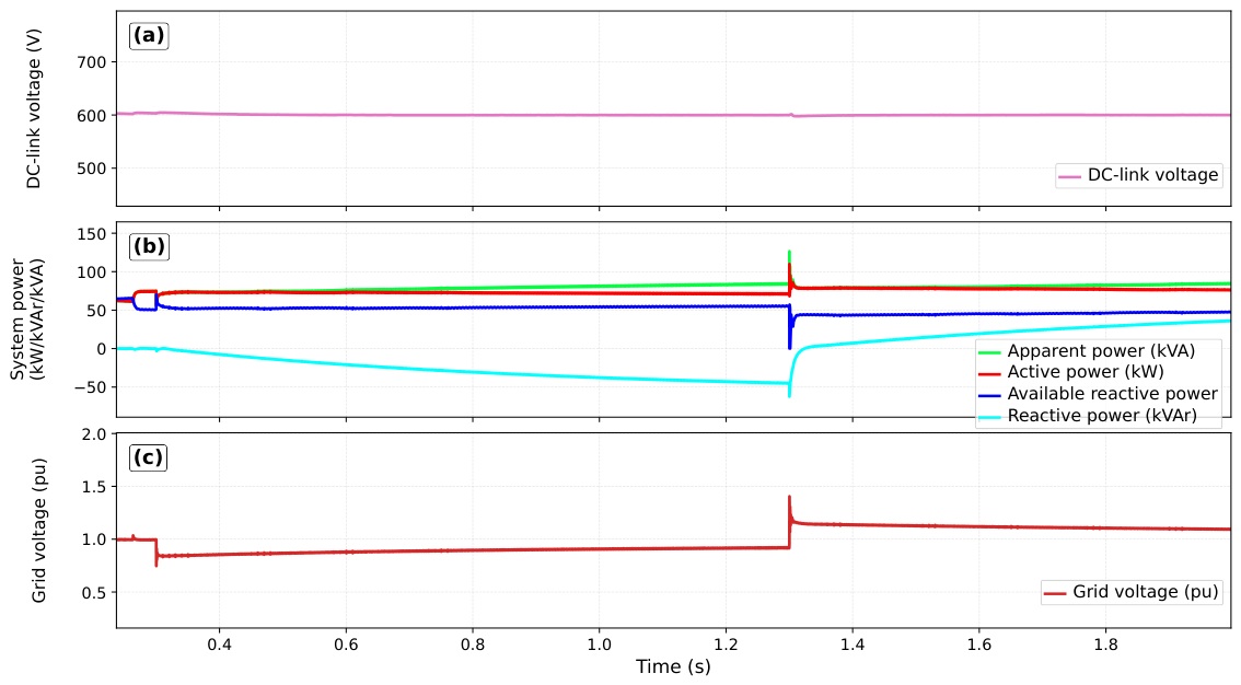
In this case, irradiance is held at 1.00 pu from $t=0$ to $t=1.5$ s and steps to 0.50 pu at that instant, remaining there for the rest of the window. The grid voltage shifts from 1.00 pu to 0.93 pu at $t=0.5$ s and to 1.07 pu at $t=1.0$ s; both levels remain within the Volt–VAR dead band.

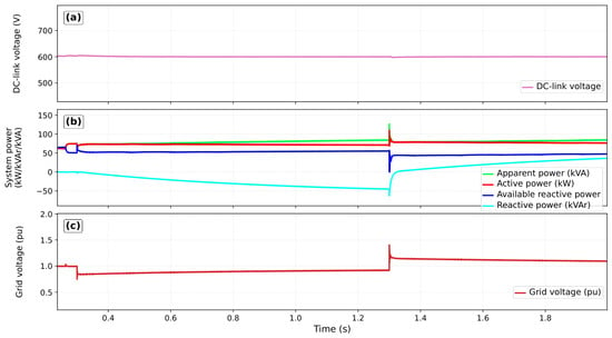
The DC bus tracks the 600 V reference throughout the scenario, as shown in Figure 12. At $t=1.5$ s, when irradiance drops abruptly by half, $V_{dc}$ deviates to a nadir of approximately 585 V, a 2.5% transient deviation from the 600 V reference, and recovers to within $\pm 2$ V of the reference in approximately 80–100 ms, consistent with the bandwidth of the BESS outer voltage loop. Active power drops from ≈80 kW to ≈40 kW, tracking the reduced PV generation. Reactive power remains near zero during both voltage disturbances, confirming the absence of Volt–VAR action within the dead band. The $Q_{disp}$ margin grows from ≈50 kVAr to ≈80 kVAr after $t=1.5$ s, with the release of apparent capacity from the lower active dispatch.

Figure 12. DC-bus voltage (V), system powers (kW, kVAr, kVA), and grid voltage (pu) in Case 1: (a) DC-bus voltage (V); (b) active, reactive, apparent power and $Q_{disp}$ (kW, kVAr, kVA); (c) grid voltage (pu).

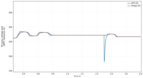
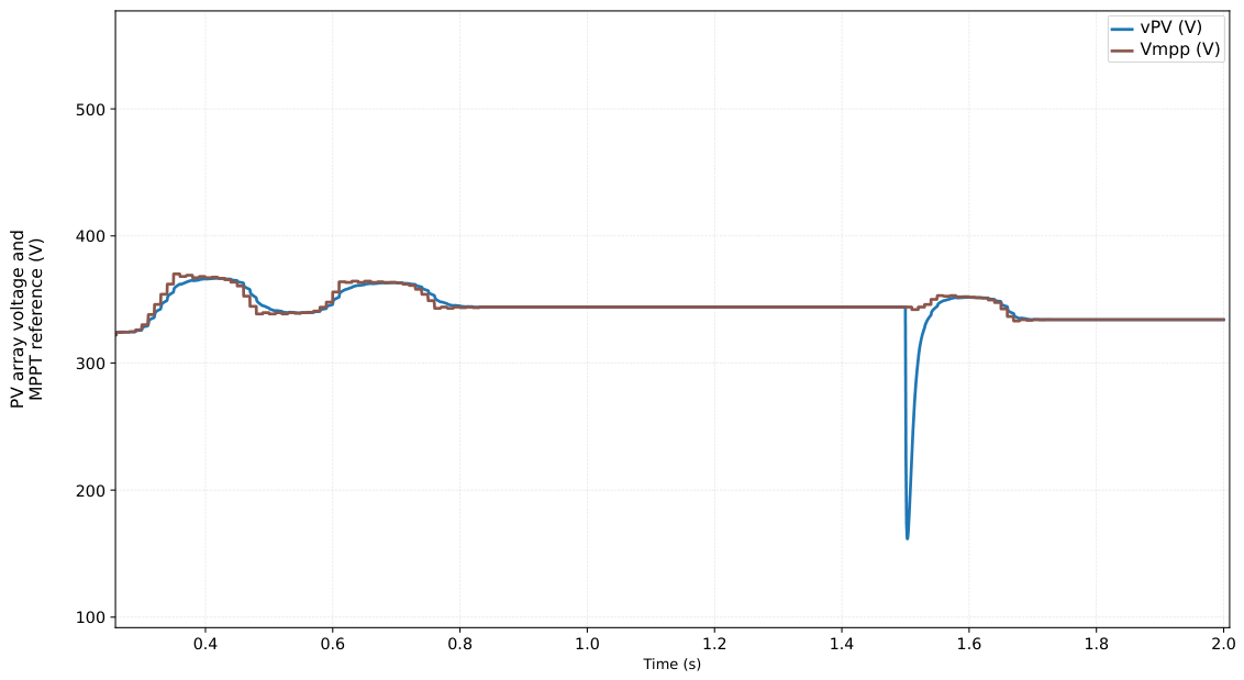
Figure 13 confirms that $v_{PV}$ and $V_{mpp}$ track together at 367 V and descend together after $t=1.5$ s. Voltage disturbances within the dead band produce no measurable effect on the PV stage. Throughout Case 1, the BESS remains completely inactive: zero currents and bank voltages stabilized at 384.00 V ($\pm 0.02$ V) and SOC at 0.800 pu.

Figure 13. PV array terminal voltage $v_{PV}$ and MPPT reference $V_{mpp}$ (V) over time in Case 1.

4.2. Case 2: Reactive Compensation Without PV Generation

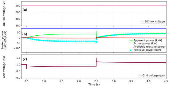
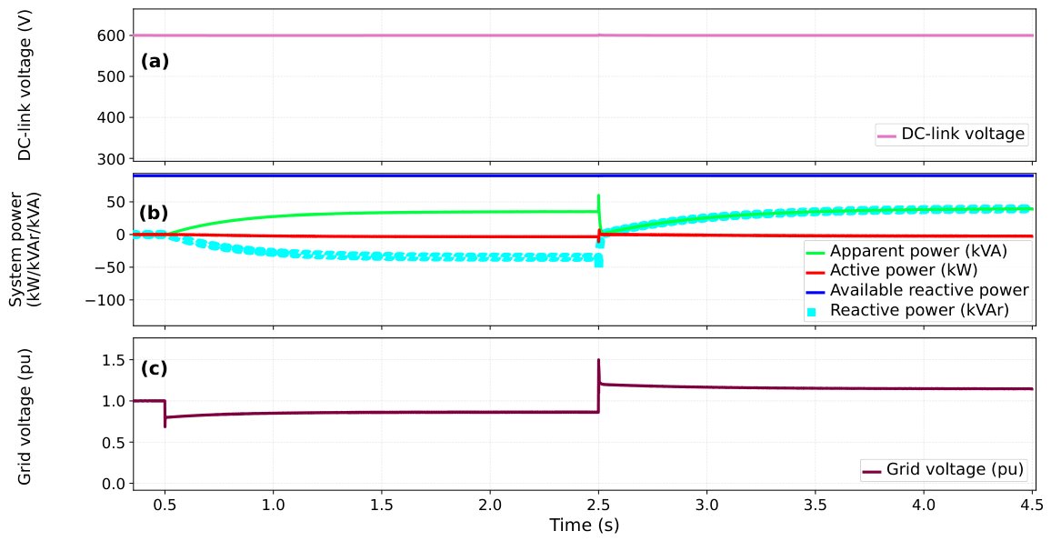
With zero irradiance, the inverter operates as a pure reactive compensator. Voltage sequence: 1.00 pu (0–0.5 s), sag to 0.80 pu (0.5–2.5 s), rise to 1.20 pu (2.5–4.5 s); the transition skips the brief return to 1.00 pu used elsewhere so that each direction gets a longer, uninterrupted window (Section 3.3 explains why this matters for the undervoltage direction).

The DC bus remains at 600 V throughout the scenario, with no measurable disturbance at either transition, as shown in Figure 14. Active power is negligible: with both the PV array and the BESS inactive, DC-bus regulation duty transfers to the VSI itself, which imports a small active current from the grid ($i_d$ slightly negative in Figure 14) to cover the LC-filter and switching losses that would otherwise discharge $C_{dc}$; this differs from Cases 1, 3, and 4, where the BESS is the active bus regulator and is not currently distinguished in Table 6. Reactive power ramps up in the negative direction throughout the undervoltage interval but never converges: it instead enters a self-sustained limit cycle around ≈$-35$ kVAr once the reactive injection raises the PCC voltage enough to trigger the supervisory logic’s fault-recovery reset, restarting the ramp from zero (mechanism detailed in Section 3.3). The overvoltage direction does not exhibit this limit cycle and settles cleanly to ≈$+39$ kVAr within ≈1.57 s of the step, faster than the 5 s default open-loop response time specified for Category B Volt–VAR in IEEE 1547-2018 [23]. The $Q_{disp}$ margin remains near 90 kVAr, confirming that the full inverter capacity is available for reactive support when $i_d$ is zero.

Figure 14. DC-bus voltage (V), system powers, and grid voltage (pu) in Case 2: (a) DC-bus voltage (V); (b) active, reactive, apparent power and $Q_{disp}$ (kW, kVAr, kVA); (c) grid voltage (pu).

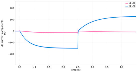
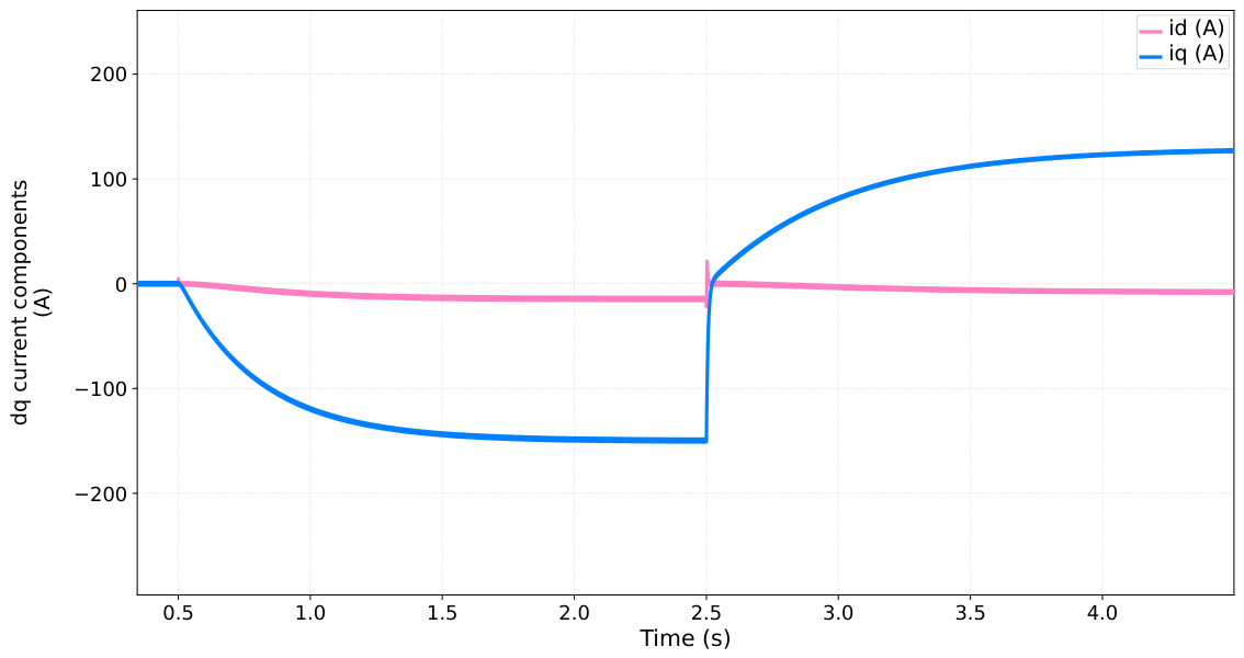
The d–q decomposition in Figure 15 confirms clean channel separation: $i_d$ remains near zero throughout, while $i_q$ reaches ≈$-150$ A during the undervoltage (limit-cycle bound, per the discussion above) and settles at ≈$+125$ A during the overvoltage. The sign reversal of $i_q$ follows the voltage step at $t=2.5$ s. The SOC asymmetry across banks stays below 0.002 pu, attributable to asymmetric residual currents in the inductors, not a systematic estimation error.

Figure 15. Inverter $i_d$ and $i_q$ components in Case 2 (A).

4.3. Case 3: Grid Voltage Steps with Full PV Generation

Irradiance is held at 1.00 pu. The grid voltage steps to 0.85 pu at $t\approx 0.3$ s and to 1.15 pu at $t\approx 1.3$ s, requiring the inverter to simultaneously process ≈90 kW and deliver reactive support.

The DC bus remains at 600 V throughout the scenario, as shown in Figure 16. Reactive power reaches $-55$ kVAr at the end of the undervoltage interval and $+50$ kVAr after the overvoltage step. The $Q_{disp}$ margin is 45–55 kVAr, ≈40 kVAr below Case 2, because unrestricted $i_d$ occupies a significant fraction of the inverter’s apparent capacity. With $P\approx 90$ kW and $\left|Q\right|$ up to 55 kVAr simultaneously, $S=\sqrt{P^2+Q^2}\approx 105 \mathrm{k}\mathrm{V}\mathrm{A}$ transiently exceeds $S_{nom}\approx 91 \mathrm{k}\mathrm{V}\mathrm{A}$; this scenario is deliberately left unconstrained beyond the vector-magnitude circle limiter of Section 3.4, exposing a transient overload (independently confirmed at 101.5% of $I_{MAX\_INV}$ from the raw current trace) rather than an internally inconsistent operating point. The PV array operates near 90 kW with $v_{PV}$ and $V_{mpp}$ fixed at 367 V during both disturbances; AC-side disturbances produce no measurable effect on the PV stage. The BESS remains inactive.

Figure 16. DC-bus voltage (V), system powers, and grid voltage (pu) in Case 3: (a) DC-bus voltage (V); (b) active, reactive, apparent power and $Q_{disp}$ (kW, kVAr, kVA); (c) grid voltage (pu).

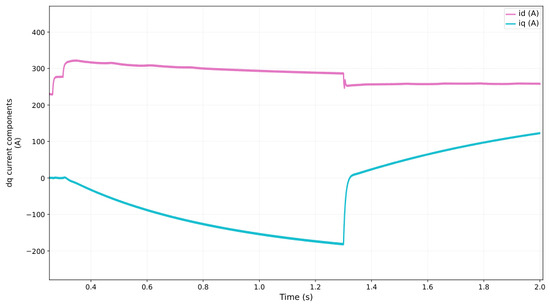
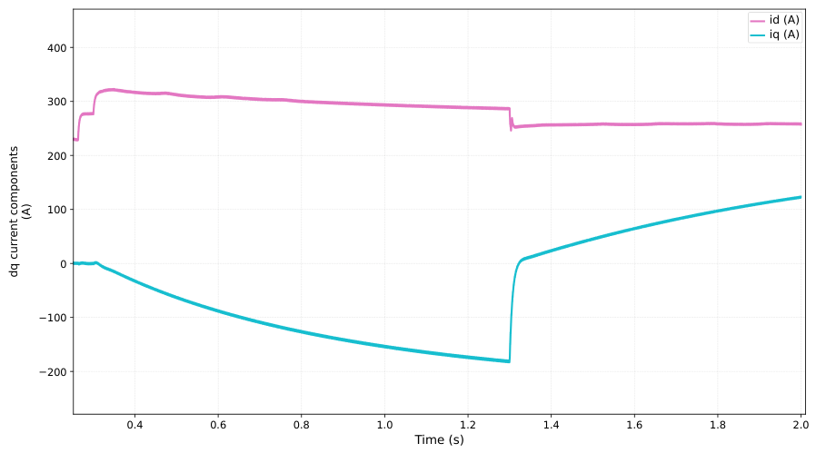
The d–q components of Figure 17 show $i_d$ ranging from 250 to 320 A. During undervoltage, $i_q$ reaches $-190$ A; during overvoltage, it reaches $+120$ A. The 2.5:1 dominance of $i_d$ over $i_q$ quantifies the reactive support penalty of unconstrained active current injection under full PV generation; Case 4 (Section 4.4) shows how redirecting active power to BESS charging, rather than an externally imposed current limit, achieves a comparable expansion of the reactive margin. These $i_d$ magnitudes are consistent with the nominal $\approx 180 \mathrm{V}$ grid phase peak voltage confirmed for this model (Section 2.3): applying $P\approx {\displaystyle \frac{3}{2}}{v}_d{i}_d$ with $v_d\approx 180 \mathrm{V}$ reproduces the reported 250–320 A range for $P=80$–100 kW (predicted $i_d\approx 296$–370 A, matching within the expected variation from the simultaneous $i_q$ contribution and the voltage-step dynamics within the window), and is independently confirmed by solving $P={\displaystyle \frac{3}{2}}(v_d{i}_d+v_q{i}_q)$, $Q={\displaystyle \frac{3}{2}}(v_d{i}_q-v_q{i}_d)$ for $v_d,v_q$ directly from the raw Case 3 simulation data ($P=71.8$ kW, $Q=-10.9$ kVAr, $i_d=310.5$ A, $i_q=-42.4$ A at $v_{grid,pu}=0.856$), which yields $v_d\approx 154.5$ V, $v_q\approx 2.3$ V, i.e., a nominal (1.0 pu) $v_d\approx 180.5 \mathrm{V}$, matching the confirmed grid voltage exactly. The filter design current in Section 2.3, based on the confirmed 220 V line voltage (peak line current ≈$337.7 \mathrm{A}$), comfortably covers the $i_d$ range reported here.

Figure 17. Inverter $i_d$ and $i_q$ components in Case 3 (A).

4.4. Case 4: Bidirectional Voltage Support and BESS Charging Under Sustained Disturbances

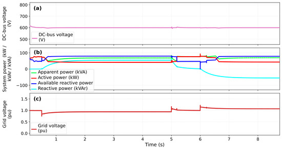
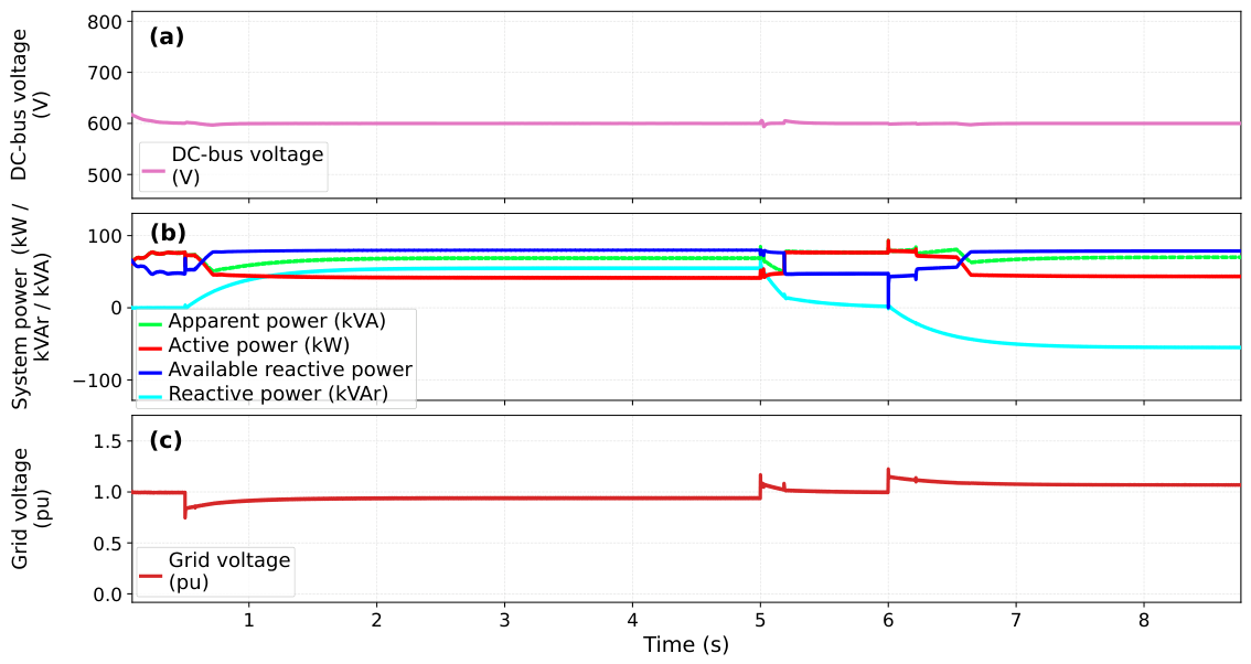
This scenario evaluates, over a 9 s window, the coordinated response of PV generation at maximum power, bidirectional Volt–VAR support, the inverter’s current-vector limiter, and BESS charging under two sequential grid-voltage disturbances. Irradiance is held at 1.00 pu with MPPT and the Boost stage continuously active. Grid voltage follows a programmed sequence: nominal until $t=0.5$ s; sag to 0.80 pu from $t=0.5$ s to $t=5.0$ s (undervoltage segment); return to nominal from $t=5.0$ s to $t=6.0$ s (an accommodation interval, not itself an analyzed steady state), and rise to 1.20 pu from $t=6.0$ s to $t=9.0$ s (overvoltage segment). The BESS is initialized at 50% SOC (≈350 V). No active-current limit is imposed externally: the supervisory logic enforces the vector-magnitude constraint $I_{dq}=\sqrt{i_d^2+i_q^2}\le I_{MAX\_INV}=335 \mathrm{A}$ (Section 3.4), so that $i_{d,max}=\sqrt{I_{MAX\_INV}^2-i_q^2}$ shrinks dynamically as reactive demand $|i_q|$ grows. The excess PV power $P_{exc}=max(P_{PV}-\left|P_{out}\right|,0)$ is redirected to BESS charging in both disturbance segments, so the bank acts as an energy buffer for the current-vector limiter under undervoltage as well as overvoltage.

The DC bus remains regulated near 600 V throughout (Figure 18), with only brief deviations at the three step instants before recovering within a few grid cycles, confirming that the active power withheld from the PCC is absorbed by the BESS rather than accumulating on the DC-link capacitor. In the undervoltage segment, PCC active power reduces progressively and stabilizes near 42 kW while reactive power grows to ≈$55 \mathrm{k}\mathrm{V}\mathrm{A}\mathrm{r}$ injected (positive, per this work’s sign convention); apparent power settles between 68 and 69 kVA and $Q_{disp}$ rises to ≈$80 \mathrm{k}\mathrm{V}\mathrm{A}\mathrm{r}$, the withheld active power corresponding not to lost generation but to PV surplus redirected to BESS charging (detailed below). Between $t=5.0$ and $6.0$ s, as the grid returns to nominal, reactive demand tends to zero, active power recovers to ≈76–78 kW, and BESS charging current drops to near zero, a temporary decoupling of the storage stage before the second disturbance. The overvoltage segment mirrors this pattern with the reactive-power sign inverted: active power converges to ≈$44 \mathrm{k}\mathrm{W}$, reactive power reaches $-53$ to $-55 \mathrm{k}\mathrm{V}\mathrm{A}\mathrm{r}$ (absorption), apparent power remains near 69 kVA, and $Q_{disp}$ returns to ≈$78 \mathrm{k}\mathrm{V}\mathrm{A}\mathrm{r}$, again freeing the current-vector margin for Volt–VAR support while the PV surplus is absorbed by the bank.

Figure 18. DC-bus voltage (V), system powers, and grid voltage (pu) in Case 4: (a) DC-bus voltage (V); (b) active, reactive, apparent power and $Q_{disp}$ (kW, kVAr, kVA); (c) grid voltage (pu).

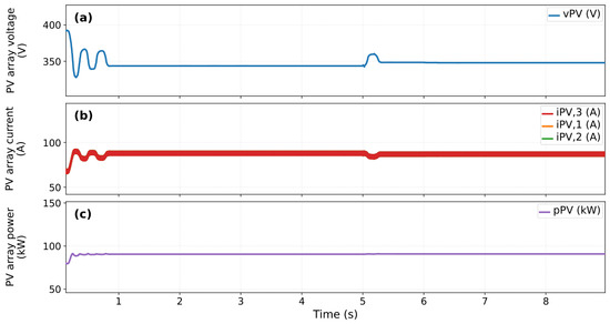
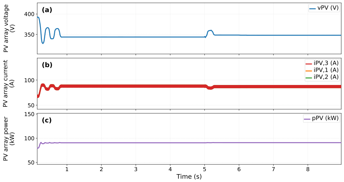
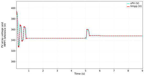
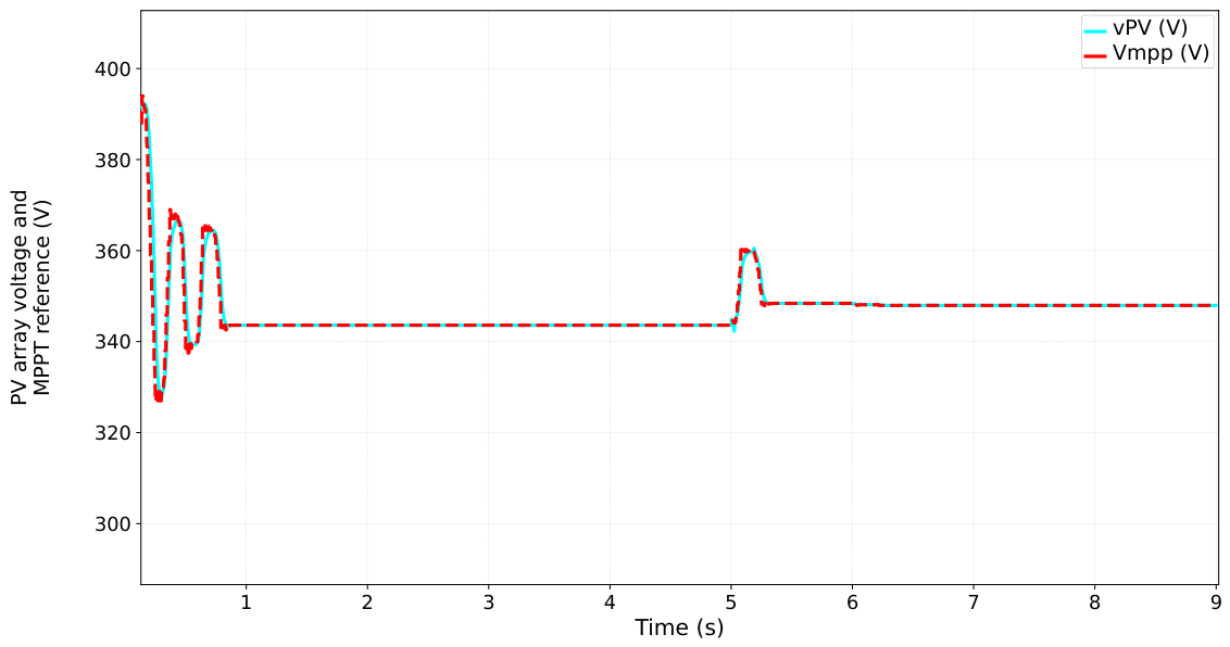
Because the grid source is not an ideal step, the measured PCC voltage evolves within each segment: it bottoms near 0.80 pu immediately after the undervoltage step and rises progressively to ≈0.94 pu as the growing reactive injection provides partial voltage support, while in the overvoltage segment, after the transient peak, growing reactive absorption pulls it back down to a steady ≈1.07 pu, a measurable effect on the PCC voltage in both directions, not merely a reactive reference. The PV array (Figure 19) operates essentially undisturbed by these grid events: after the initial transient, $v_{PV}$ stabilizes near 343 V, the three branch currents remain balanced near 88–90 A, and array power converges to ≈$91 \mathrm{k}\mathrm{W}$, staying practically constant for the entire window; a brief disturbance near $t=5$ s is followed by rapid recomposition of the operating point, confirming that the MPPT loop (Figure 20) tracks independently of the grid/BESS power-sharing decision. $v_{PV}$ and $V_{mpp}$ remain almost exactly superposed throughout (Figure 20): both stay near 343 V before $t=5$ s and converge to ≈$348 \mathrm{V}$ afterward, confirming that redistributing power among the inverter, the grid, and the BESS does not sustainedly displace the array from its maximum-power point.

Figure 19. Voltage (V), current (A), and power (kW) of the PV array in Case 4: (a) array voltage $v_{PV}$ (V); (b) array current (A); (c) array power (kW).

Figure 20. PV array terminal voltage $v_{PV}$ and MPPT reference $V_{mpp}$ (V) over time in Case 4.

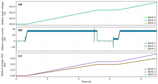
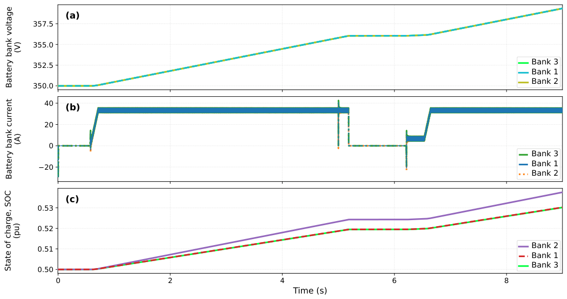
The BESS (Figure 21) is active in both disturbance segments. In the undervoltage segment, charging current rises shortly after the disturbance begins and stabilizes near 33–35 A per bank, sustained until the grid returns to nominal; bank voltage rises from ≈350 to 356 V; and SOC advances from 0.500 to ≈0.519–0.524 pu. This is not active PCC voltage support: the BESS does not discharge to raise it; rather, it charges, absorbing the PV power share withheld from the grid when $i_d$ is reduced to preserve $i_q$ priority and the inverter’s current limit, acting as an energy buffer for the DC link while preserving MPPT operation, reactive support, and $V_{dc}$ regulation. Between $t=5$ and 6 s, bank current returns to near zero and voltage/SOC remain practically constant. Charging re-enables once the overvoltage segment begins, with a brief low-current interval as the control progressively arms, followed by a rise to ≈33–35 A per bank from $t\approx 6.7$ s; by the end of the window, bank voltage approaches 359–360 V and SOC reaches ≈0.530–0.537 pu.

Figure 21. Bank voltage (V), current (A), and state of charge (pu) in Case 4: (a) bank voltage (V); (b) bank current (A); (c) bank SOC (pu).

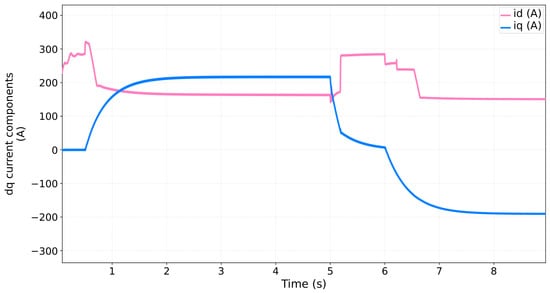
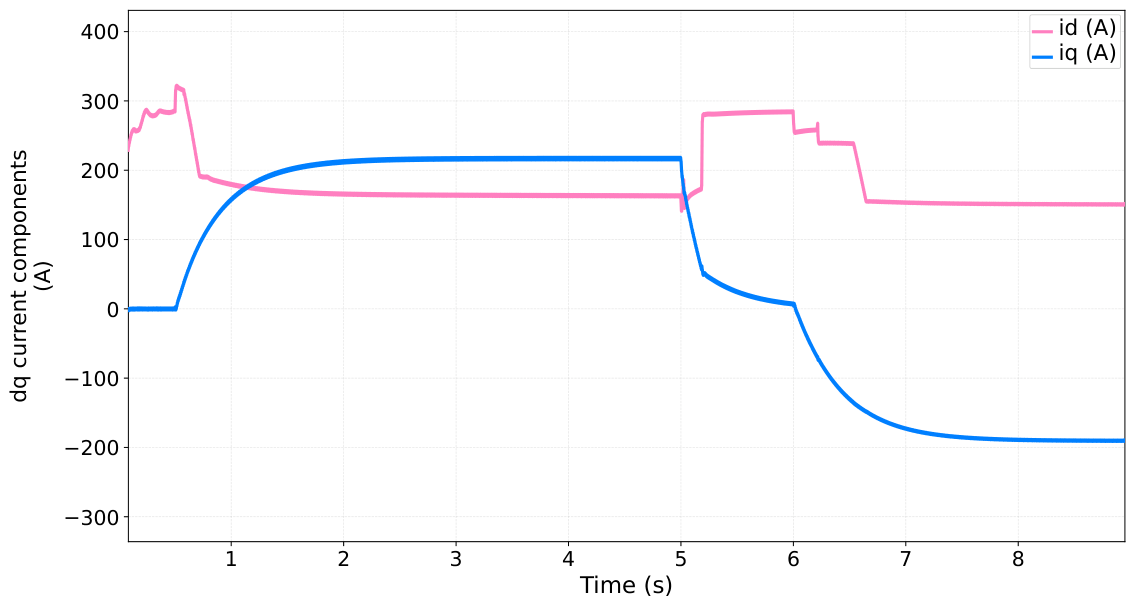
The split between active and reactive current (Figure 22) results solely from the vector-magnitude constraint together with Volt–VAR priority; no external $i_d$ limit is imposed. After the initial transients, $i_q$ grows to ≈215–218 A in the undervoltage segment while $i_d$ is correspondingly reduced to ≈163–165 A, giving $I_{dq}\approx \sqrt{{164}^2+{216}^2}\approx 271 \mathrm{A}$, comfortably below the 335 A limit: giving priority to reactive support does not cause a sustained current overrun, since the active share is reduced instead and the corresponding energy is absorbed by the BESS. During the accommodation, interval $i_q$ returns gradually toward zero and $i_d$ recovers most of the available current; in overvoltage, segment $i_q$ changes sign and converges to ≈$-188$ to $-190 \mathrm{A}$ while $i_d$ reduces to $\approx 150 \mathrm{A}$, giving $I_{dq}\approx \sqrt{{150}^2+{190}^2}\approx 242 \mathrm{A}$, again below the rated limit. This dynamic split preserves Volt–VAR priority without exceeding the converter’s current circle in either direction of the disturbance; phase voltages track the grid profile at each step without loss of three-phase balance, and the output current amplitude falls from the undervoltage to the overvoltage segment in the same proportion as $i_d$, with synchronism preserved throughout, including across the accommodation interval.

Figure 22. Inverter $i_d$ and $i_q$ components in Case 4 (A).

4.5. Case 5: Overvoltage Ride-Through with PV Curtailment and a Fully Charged Bank

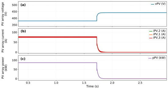
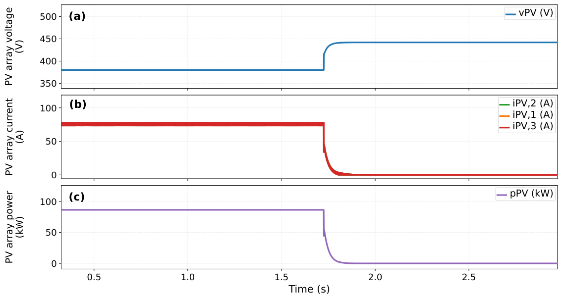
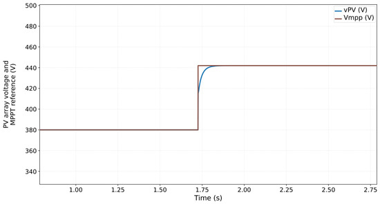
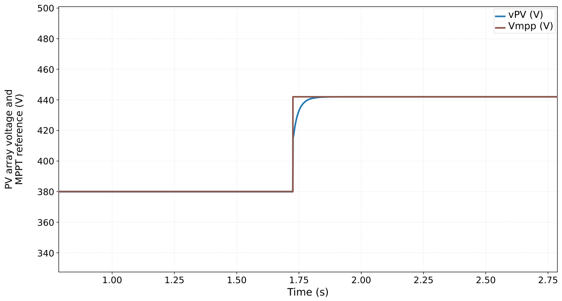
All three banks begin this scenario already saturated, at $SOC\approx 0.97$ pu (a level the supervisory logic treats as the operational ceiling), so the BESS neither charges nor discharges throughout. Irradiance is held at 1.00 pu. Grid voltage remains at 1.00 pu until $t=0.4$ s, then steps to $\approx 1.20$ pu and is sustained for the remainder of the 3 s window; unlike Cases 2–4, this scenario evaluates overvoltage exclusively, with no undervoltage segment. With the BESS unable to absorb the PV surplus, the supervisory curtailment logic limits the PV active power reference to the available export capacity once the DC bus can no longer be balanced by storage alone. Mechanistically, the P&O block continues computing $V_{mpp}$ from the array’s $v_{PV}$–$i_{PV}$ measurements as in the other scenarios, but curtailment overrides the current reference fed to the Boost outer voltage loop, clamping it below the value $V_{mpp}$ would otherwise command; the PV operating point is thereby displaced off the I–V curve’s maximum-power point even though the MPPT reference itself keeps tracking, so generation can resume at the true MPP as soon as export capacity or the storage margin becomes available again, without restarting the P&O search. Curtailment (engaging at $t\approx 1.7$ s) displaces $v_{PV}$ from ≈380 V to ≈442 V (toward the array’s open-circuit region), while the per-leg PV current collapses from ≈76 A to near zero within ≈0.1 s (see Figure 23), with $v_{PV}$ tracking $V_{mpp}$ (including the shifted reference) without overshoot (see Figure 24). In the C-Script source, the curtailment offset is added to the MPPT reference, $V_{mppt,final}=V_{mppt,base}+\mathrm{CurtOffset}$, engaging whenever $V_{dc}$ exceeds a threshold or the active/apparent-power limits are approached and recovering slowly once conditions clear. A second, discrete protection layer exists beneath it: if $V_{dc}$ continues rising to $615 \mathrm{V}$ despite maximum curtailment, the Boost PWM itself is latched off entirely (independent of the continuous $\mathrm{CurtOffset}$ path) until $V_{dc}$ recovers below $602 \mathrm{V}$ for a minimum hold time, the same mechanism behind the secondary protection event identified in the extended HIL observation window (Section 4.7): once curtailment saturates at its $\mathrm{CURT}\_\mathrm{MAX}$ limit and $V_{dc}$ keeps rising, this discrete latch interrupts PV generation entirely.

Figure 23. Voltage (V), current (A), and power (kW) of the PV array in Case 5: (a) array voltage $v_{PV}$ (V); (b) array current (A); (c) array power (kW).

Figure 24. PV array terminal voltage $v_{PV}$ and MPPT reference $V_{mpp}$ (V) over time in Case 5.

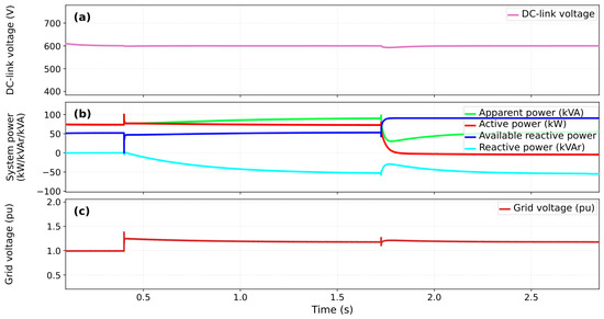
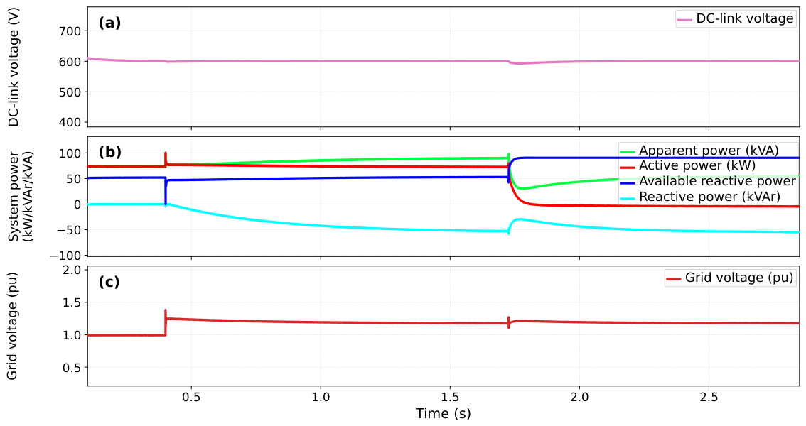
The DC bus tracks the 600 V reference throughout the scenario, as shown in Figure 25, with only a momentary dip to ≈592.6 V ($-7$ V, $-1.2\%$) at the curtailment instant ($t\approx 1.77$ s), settling back to within $\pm 2$ V of the reference within ≈150–200 ms. Between the voltage step and the curtailment instant, reactive power grows continuously in the negative (inductive-absorption) direction, from near zero to ≈$-55$ kVAr, as the Volt–VAR loop responds to the sustained overvoltage; active power remains near 75–87 kW in this interval. At $t\approx 1.7$ s, curtailment engages: active power collapses to near zero and $Q_{disp}$ jumps from ≈50 kVAr to ≈90 kVAr, releasing nearly the full inverter capacity for reactive support. The grid voltage measured at the PCC settles near 1.20 pu immediately after the step and decreases gradually to ≈1.17 pu over the remainder of the window, evidencing the (partial) voltage-support effect of the inductive reactive injection despite the ideal-source representation discussed in Section 3.3.

Figure 25. DC-bus voltage (V), system powers, and grid voltage (pu) in Case 5: (a) DC-bus voltage (V); (b) active, reactive, apparent power and $Q_{disp}$ (kW, kVAr, kVA); (c) grid voltage (pu).

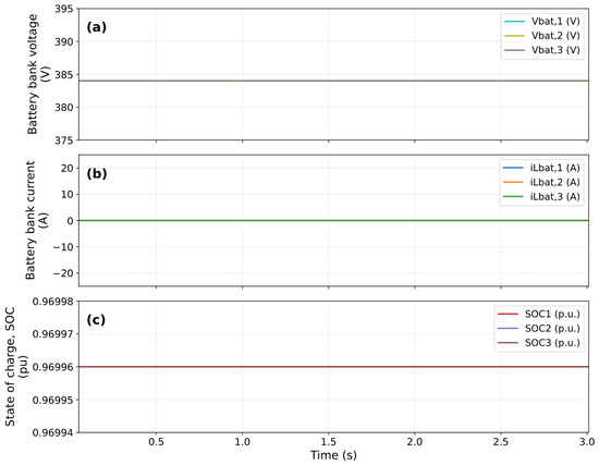
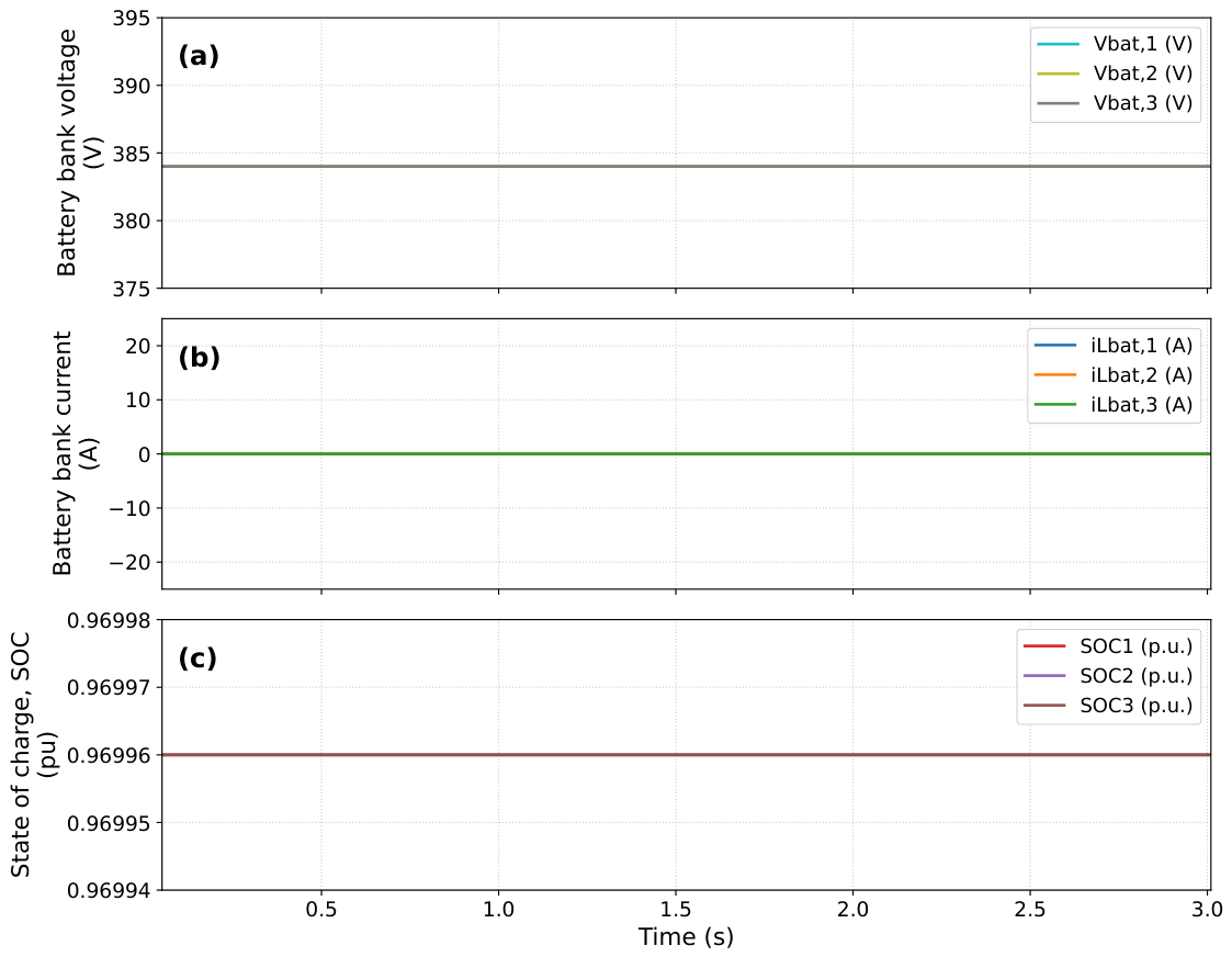
Bank voltages remain stable near 384 V throughout, currents stay near zero, and SOC values remain confined to the range 0.96994–0.96998 pu (Figure 26), with the $4\times {10}^{-5}$ pu span across the three banks reflecting asymmetric residual inductor currents, not a systematic estimation error. The P&O algorithm continues to execute; curtailment acts on the active power reference, not on the tracking algorithm, preserving MPPT integrity for when storage margin becomes available again.

Figure 26. Bank voltage (V), current (A), and state of charge (pu) in Case 5: (a) bank voltage (V); (b) bank current (A); (c) bank SOC (pu).

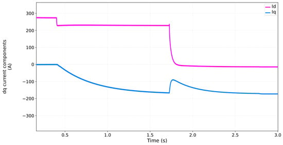
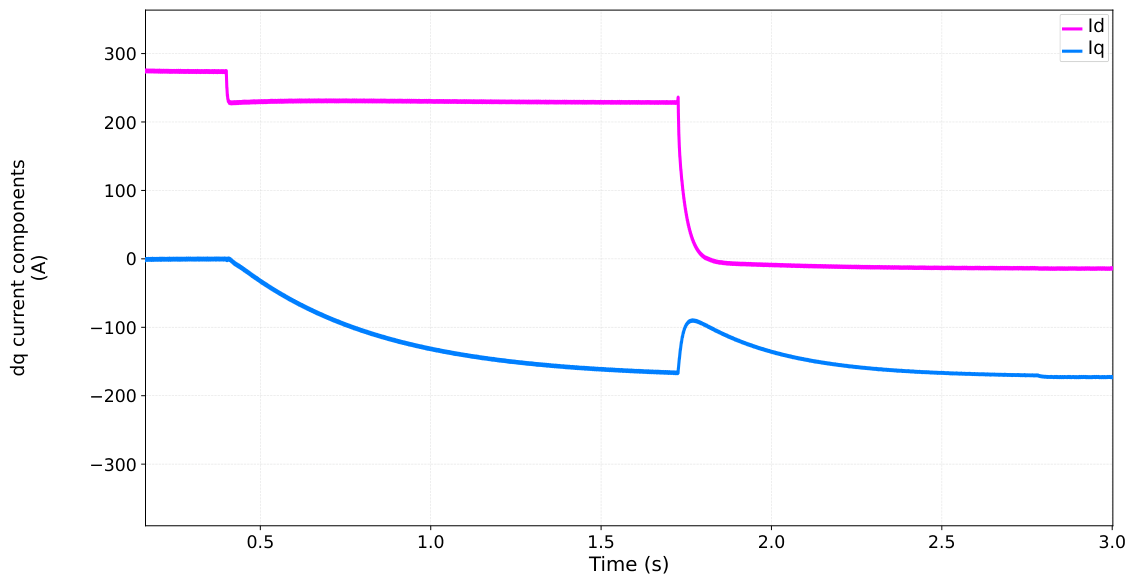
Figure 27 shows $i_d$ settling near 275 A during the initial 1.00 pu interval, decreasing to ≈230 A after the voltage step (the same active power at a higher grid voltage requires less $i_d$), and decaying to near zero once curtailment engages. The reactive component $i_q$ remains near zero before the step, then grows steadily in magnitude, with a brief reduction to ≈$-90$ A at the curtailment instant before resuming toward ≈$-175$ A by the end of the window, staying negative throughout, consistent with a scenario restricted to overvoltage. The inverter line current peaks near 280 A before curtailment and, after the active-power collapse, reorganizes into an envelope growing from ≈100 A to ≈180 A as $|i_q|$ increases, current that is by then almost entirely reactive, with no measurable disruption to reactive support capacity, confirming that the supervisory logic successfully decouples the active-power protection function from the reactive-power control path.

Figure 27. Inverter $i_d$ and $i_q$ components in Case 5 (A).

The longer observation window used during HIL validation of this scenario (beyond the 3 s PLECS window presented above) additionally revealed a secondary protection event: once curtailment alone can no longer contain the PV surplus with a permanently saturated bank, PV generation is interrupted entirely (Boost current and active power fall to zero), while Volt–VAR reactive support remains active throughout. This event is part of the same Case 5 validation window (not a sixth scenario) and was reproduced at the same relative instant in both the PLECS and HIL environments, as detailed in Section 4.7.

4.6. Summary of Results

Table 7 consolidates the main quantitative results, including the transient metrics extracted from the simulated waveforms.

Table 7. Summary of simulation results across the five scenarios. Transient metrics were extracted directly from the simulated waveforms.

Case	Nadir/Overshoot of ${\mathit{V}}_{\mathit{dc}}$	${\mathit{V}}_{\mathit{dc}}$ Settling	Q Range (kVAr)	${\mathit{Q}}_{\mathit{disp}}$ (kVAr)
1 (irradiance step)	585 V ($-2.5\%$)	≈80–100 ms	≈0	50–80
2 (reactive only, no PV)	600 V	—	$-35$ to $+39$ ‡	≈90
3 (full PV + steps)	600 V	—	$-55$ to $+50$	45–55
4 (bidirectional, 9 s) §	$-6.5$/$+20.1$ V	few grid cycles	$-55$ to $+55$	78–80
5 (OV ride-through, curt.)	$-7$ V ($-1.2\%$) †	≈150–200 ms †	0 to $-55$	50–90

Note: settling time measured to $\pm 2$ V from the 600 V reference. ^† Case 5’s $V_{dc}$ dip magnitude and settling time at the curtailment instant (Section 4.5) are extracted directly from the HIL scope trace (nadir ≈592.6 V at $t\approx 1.77$ s, settling to within $\pm 2$ V by $t\approx 1.93$ s), closely reproducing the corresponding PLECS waveform. ^‡ Case 2’s Q range uses an extended disturbance window (Section 3.3): the overvoltage value ($+39$ kVAr) is a settled reading ($\pm 2\%$, reached in ≈1.57 s); the undervoltage value ($-35$ kVAr) is the value reached within the ≈2 s available before a self-sustained limit cycle (grid-voltage-triggered reset interacting with the non-zero grid-side coupling impedance) restarts the ramp, and it is not a converged steady-state value. ^§ Case 4’s Q range and $Q_{disp}$ are the steady-state values of each 4.5 s disturbance segment (Section 4.4); brief transients immediately after each step are absorbed by the current-control loop within a few cycles.

Case 2’s disturbance window is long enough to test whether Q reaches a genuine steady state, revealing a genuine control interaction rather than a simple window-length limitation: the supervisory logic instantly discharges the reactive accumulator ($I_{comp}\to 0$) whenever the measured PCC voltage re-enters the $0.91$–$1.09$ pu relaxation band. Because the grid-side coupling inductance ($L=200 \mathrm{\mu }\mathrm{H}$/phase, the same non-zero impedance used in the weak-grid test above) makes the reactive injection itself raise the PCC voltage, a sustained undervoltage condition drives Q high enough to push the PCC voltage back across the relaxation threshold, triggering the reset and restarting the ramp from zero, a self-sustained limit cycle (≈2 s period) rather than convergence to a fixed value, and a genuine emergent behavior under non-ideal grid coupling, not a simulation artifact; the overvoltage direction does not exhibit it and settles cleanly instead. Section 4.2 reports the measured values (Figure 14 and Figure 15) from this extended-window test. This limit cycle is reported here as a known characteristic of the current reset logic rather than mitigated with an additional hysteresis band, which would require new PLECS re-simulation and HIL re-validation beyond the scope of this study; it is noted as a direction for future controller refinement.

In all cases but Case 4, $V_{dc}$ remained within $\pm 15$ V of the 600 V reference (Table 7); the largest transient deviation, a 15 V drop in Case 1, recovered in approximately 80–100 ms. Case 4’s step transients stay within $-6.5$/$+20.1 \mathrm{V}$ of the 600 V reference and recover within a few grid cycles each time, consistent with the well-damped $V_{dc}$ loop exercised over its longer, 9 s bidirectional window; its steady-state $Q_{disp}$ reaches ≈78–80 kVAr in both disturbance segments, as PV surplus is redirected to BESS charging under both undervoltage and overvoltage, with charging current stabilizing at 33–35 A per bank, achieved without any externally imposed active-current limit and with the current-vector magnitude confirmed below 335 A throughout (≈271 A/≈242 A). Case 5 demonstrates that curtailment eliminates the DC-bus overvoltage risk with a saturated, fully charged bank under a sustained overvoltage ride-through (1.00 to 1.20 pu), with only a brief $V_{dc}$ dip at the curtailment instant, while $Q_{disp}$ rises from ≈50 to ≈90 kVAr, showing that Volt–VAR capacity is not only preserved but substantially expanded once active power is curtailed.

The metrics above characterize transient behavior but stop short of the steady-state power-quality and loading indicators expected of a grid-interface study. Table 8 completes this picture by post-processing the same PLECS traces (no new simulation) for injected-current RMS and THD, VSI and BESS loading margins, and DC-bus ripple, in all five cases.

Table 8. Injected-current quality and converter loading margins, post-processed from the switching-resolution simulation traces of each case.

Case	RMS (A)	THD (5% Limit)	VSI Margin	BESS Margin	DC Ripple (kHz/V)
1	135.5	0.012% pass	59.3%	—	36.0/0.58
2 †	85.2/52.1	0.41/0.94% pass	49.5%	—	18.2/0.12
3	232.3/191.6	0.16/0.29% pass	101.5% ‡	—	17.8/0.60
4	191.9/171.2	0.05/0.01% pass	81.4/72.8%	33.3/33.3%	18.2–36.0/ 0.28–0.17
5	190.5/118.2	0.11/0.05% pass	84.8%	—	36.0–17.8/ 0.46–0.25

Paired values are undervoltage/overvoltage (Cases 2, 3) or pre-/post-curtailment (Case 5). RMS/THD computed over an integer number of 60 Hz cycles in the steady-state portion of each disturbance; THD sums the 2nd–40th harmonics per the IEEE 1547-2018 convention (5% limit, which by design excludes switching-frequency content). VSI/BESS margins are the peak current as a percentage of $I_{MAX\_INV}=335 \mathrm{A}$ and $I_{BAT,REF\_MAX}=100 \mathrm{A}$/bank, respectively; the BESS margin is marked where the bank is inactive or saturated in that case. ^† Full-resolution phase-current data for the specific $4.5$ s extended-disturbance window of Case 2 (Section 3.3) was not available in the archived traces; the values shown come from a shorter, full-resolution run of the same undervoltage/overvoltage scenario and should be read as representative of injected-current quality, not as a precise measurement at the reported limit-cycle operating point. ^‡ Case 3’s 101.5% VSI loading (peak 340 A) is the transient overload already discussed in Section 4.3 ($S\approx 105 \mathrm{k}\mathrm{V}\mathrm{A}$ momentarily exceeding $S_{nom}$), independently corroborated here from the raw current trace, and is bounded only by the vector-magnitude circle limiter of Section 3.4. Case 4’s paired values are undervoltage/overvoltage segments, computed from real switching-resolution phase-current traces (fundamental amplitude cross-checked against the $dq$-derived $\sqrt{i_d^2+i_q^2}$ to within 2 A in both segments).

Efficiency and conduction/switching losses could not be reliably estimated from the available traces: none of the logged runs pair DC-side input power with AC-side output power at matching time alignment, and the PLECS model does not appear to be instrumented for loss accounting (consistent with the near-ideal switch representation used throughout this study).

4.7. Hardware-in-the-Loop Corroboration

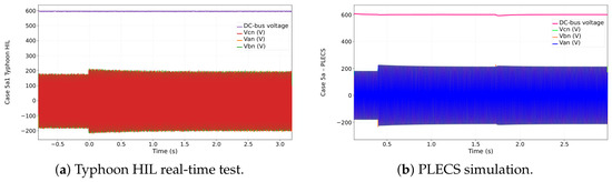
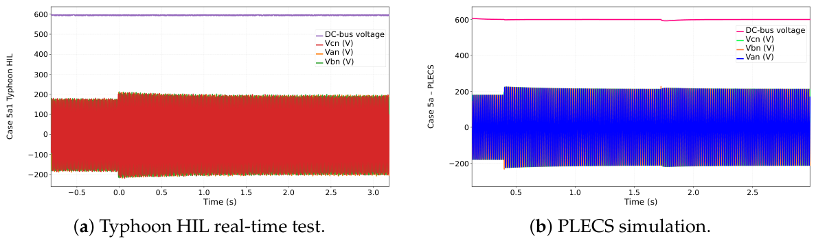
All five scenarios were repeated on a Typhoon HIL402 Pro 2 real-time platform and compared against the corresponding PLECS waveforms, following the same base conditions and disturbance sequence described above. Voltages, currents, and active/reactive power were captured with three synchronized Agilent Technologies InfiniiVision MSO-X 3014A oscilloscopes per case, reading the HIL analog outputs at fixed voltage-to-quantity scale factors. A representative comparison for Case 5 is shown in Figure 28; the full oscilloscope-by-oscilloscope record for all five cases is reported in the source dissertation.

Figure 28. Phase voltages and DC-bus voltage during the Case 5 overvoltage step: Typhoon HIL real-time test (a) versus PLECS simulation (b).

In Case 1, the DC bus remained regulated at 600 V and the phase voltages tracked the 127 V RMS/180 V peak nominal level in both environments; the current transient following the 50% irradiance step recovered within ≈30 ms on the real-time platform, consistent with the PLECS response. In Case 2, the DC bus stayed at 600 V throughout both the undervoltage and overvoltage disturbances, while the line currents and reactive power ramped up gradually and symmetrically in the HIL captures, matching the integral action of the Volt–VAR controller observed in simulation, with the BESS and PV stages confirmed inactive in both environments. Case 3 reproduced the same 600 V bus regulation together with sustained PV power near 90 kW and Boost current near 85–90 A across both voltage disturbances, with the BESS remaining inactive in both environments. Case 4 reproduced stable bus regulation across both the undervoltage and overvoltage steps, together with the gradual, symmetric reactive power evolution, and confirmed that BESS charging begins at the same relative instant as the active-power reduction in both environments. Case 5 confirmed 600 V bus regulation during the sustained overvoltage ride-through with a saturated BESS, effective PV curtailment near 90 kW immediately after the step, and (using a longer HIL observation window than the original PLECS analysis) the same secondary protection event described in Section 4.5: PV generation is fully interrupted once curtailment alone can no longer contain the surplus with a permanently saturated bank, reproduced at the same relative instant in both environments, while Volt–VAR support remains active throughout.

Across all five cases, the discrepancies between the two environments were limited to small amplitude differences in the transients, attributable to the different simulation time-step and switching-model resolution between PLECS and the Typhoon real-time solver, without affecting the qualitative or quantitative agreement of the operating regimes.

5. Conclusions

A 91 kWp three-phase photovoltaic architecture with BESS integration was modeled, implemented, and evaluated through five simulation scenarios in PLECS. Three findings are stated precisely.

The DC-bus regulation strategy maintained the 600 V reference within $\pm 15$ V in all five scenarios. The worst transient deviation, a 15 V drop during a 50% irradiance step in Case 1, recovered in approximately 80–100 ms, consistent with the bandwidth of the outer voltage loop. Coordinated bidirectional operation in Case 4 kept the DC bus close to its 600 V reference across the three step instants over its 9 s window, with only brief deviations recovering within a few grid cycles each time, within the safe operating range of the bus capacitors.

The Volt–VAR function correctly inverted reactive power between undervoltage and overvoltage in all scenarios with PCC excursion. With no externally imposed active-current limit, Case 4 sustained $Q_{disp}\approx$ 78–80 kVAr in both disturbance segments by redirecting PV surplus to BESS charging in each direction (≈33–35 A per bank), keeping the current-vector magnitude below the 335 A rating throughout (≈271 A under undervoltage; ≈242 A under overvoltage). This demonstrates that the same reactive-margin expansion achieved by active-current restriction in Case 3’s overload condition (Section 4.3) also arises naturally, and without any sustained current-limit violation, from SOC-based power coordination.

The supervisory curtailment of Case 5 prevented DC-bus overvoltage under a sustained overvoltage ride-through (1.00 to 1.20 pu) with a saturated, fully charged bank. Bank voltages remained stable near 384 V and SOC values within $4\times {10}^{-5}$ pu across three independent banks, confirming the accuracy of the per-bank coulometric estimator. The reactive channel not only remained fully operational throughout the curtailment state but gained capacity, with $Q_{disp}$ rising from ≈50 to ≈90 kVAr once active power was curtailed.

Four limitations delimit the scope of these conclusions. The results reported above are based on PLECS simulations, but all five scenarios were additionally corroborated by hardware-in-the-loop validation on the Typhoon HIL402 Pro 2 platform (Section 4.7). The grid is represented as an ideal voltage source with a prescribed voltage profile in the five main scenarios; this isolates and validates the inverter’s commanded-current tracking and the DC-bus/BESS dynamics, but, because an ideal source is by construction insensitive to reactive injection, it does not by itself demonstrate PCC voltage support on the low-SCR rural feeders that motivate this work (Section 1). A dedicated weak-grid Thévenin-equivalent test ($SCR=10,5,2$, Section 3.3) directly addresses this: PCC voltage deviation for the same disturbance grows monotonically from ≈1.13 to ≈1.27 pu as $SCR$ drops from 10 to 2, and the $SCR=2$ case additionally reveals a sustained low-frequency (≈9–12 Hz) $V_{dc}$ oscillation absent at higher SCR, evidence that the present tuning approaches its stability margin on very weak feeders and would require re-tuning or feed-forward compensation before deployment at $SCR\lesssim 2$. The SRF-PLL operates reliably under the balanced, undistorted conditions of the five main scenarios; a dedicated test with a 2% negative-sequence imbalance injected into the grid source (Section 3.3) confirmed, via FFT, a genuine 120 Hz $V_{dc}$ ripple that the SRF-PLL cannot attenuate, with peak-to-peak amplitude of only ≈0.13–0.18 V once isolated with a 100–140 Hz band-pass filter (Figure 8), two orders of magnitude smaller than a simplified analytical upper bound of 8–15 V, which does not capture the attenuating effect of the large $C_{dc}=12 \mathrm{m}\mathrm{F}$ bus capacitance. This small ripple adds to, rather than replaces, the balanced-grid transient envelope of $\pm 15$ V already reported in Table 7. A DSOGI-PLL, which would eliminate this sensitivity entirely, is reserved for future work. The LC filter provides adequate quality for the simulated scenarios, but an LCL topology would offer superior attenuation of the harmonics in the current injected into the grid.

Future steps include extending hardware-in-the-loop validation to weak-grid and unbalanced-voltage conditions, re-tuning or adding feed-forward compensation to remove the $V_{dc}$ oscillation observed at $SCR=2$ (Section 3.3), DSOGI-PLL integration, extension of the Volt–VAR function to frequency response, analysis of system behavior under partial shading on the PV array, and reporting of the small-signal loop parameters and quantitative power-quality metrics identified as pending in Section 3.4 and Section 4.6.

References

- Teodorescu, R.; Liserre, M.; Rodríguez, P. Grid Converters for Photovoltaic and Wind Power Systems; Wiley–IEEE Press: Chichester, UK, 2011. [Google Scholar]
- Empresa de Pesquisa Energética (EPE). Balanço Energético Nacional 2025—Base Year 2024; EPE: Rio de Janeiro, Brazil, 2025. [Google Scholar]
- PVPS, I.E.A. Snapshot of Global PV Markets 2024; IEA PVPS T1-47:2024; IEA: Paris, France, 2024. [Google Scholar]
- SolarPower Europe. Global Market Outlook for Solar Power 2025–2029; SolarPower Europe: Brussels, Belgium, 2025. [Google Scholar]
- Saleem, M.I.; Saha, S.; Izhar, U.; Ang, L. Stability Assessment of Inverter-Based Renewable Energy Sources Integrated to Weak Grids. IET Energy Syst. Integr. 2024, 6, 525–544. [Google Scholar] [CrossRef] [Scilit]
- Zhu, D.; Zhou, S.; Zou, X.; Kang, Y. Improved Design of PLL Controller for LCL-Type Grid-Connected Converter in Weak Grid. IEEE Trans. Power Electron. 2020, 35, 4715–4727. [Google Scholar] [CrossRef] [Scilit]
- Wang, H.; Chen, Q.; Zhang, L.; Yin, X.; Zhang, Z.; Wei, H.; Chen, X. Research and Engineering Practice of Var-Voltage Control in Primary and Distribution Networks Considering the Reactive Power Regulation Capability of Distributed PV Systems. Energies 2025, 18, 2135. [Google Scholar] [CrossRef] [Scilit]
- Fan, Y.; Yang, Y.; Wu, F.; Qiu, H.; Ye, P.; Xu, W.; Zhong, Y.; Zhang, L.; Chen, Y. Coordinated Reactive Power–Voltage Control in Distribution Networks with High-Penetration Photovoltaic Systems Using Adaptive Feature Mode Decomposition. Energies 2025, 18, 2866. [Google Scholar] [CrossRef] [Scilit]
- Gebbran, D.; Mhanna, S.; Ma, Y.; Chapman, A.C.; Verbič, G. Fair Coordination of Distributed Energy Resources with Volt-Var Control and PV Curtailment. IEEE Trans. Sustain. Energy 2023, 14, 1085–1099. [Google Scholar]
- Saleem, M.I.; Savier, J.S.; Das, S. Reactive Power Control of PV Inverters in Active Distribution Grids with High PV Penetration. IEEE Trans. Power Deliv. 2023, 11, 81477–81496. [Google Scholar] [CrossRef] [Scilit]
- Polat, S.; Biyik, E.; Şekerci Öztura, H. Optimal Active and Reactive Power Scheduling for Inverter-Integrated PV and BESS Under Inverter Current Constraints. Electr. Power Syst. Res. 2025, 245, 111629. [Google Scholar] [CrossRef] [Scilit]
- Meng, Q.; Zhao, L.; She, Q.; Guo, Q.; Guo, L.; Chen, P.; Zhao, J.; Yao, W.; Gao, Y.; Wang, S.; et al. Generation–Grid–Load–Storage Coordination for a Park-Level Integrated Energy Microgrid Under New-Type Power Systems. Energy Rep. 2026, 15, 108924. [Google Scholar] [CrossRef] [Scilit]
- Bhutto, J.K.; Kumar, A.; Kamangar, S.; Arabi, A.I.A.; Hakami, H.; Mushtaque, N. Coordinated Hybrid VAR Compensation Strategy with Grid-Forming BESS and Solar PV for Enhanced Stability in Inverter-Dominated Power Systems. Sustainability 2025, 17, 10820. [Google Scholar] [CrossRef] [Scilit]
- Alshdaifat, Y.I.R.; Prasad, K.; Al-Tameemi, Z.H.A.; Kilby, J.; Lie, T.T. Optimal Energy Storage Management in Grid-Connected PV-Battery Systems Based on GWO-PSO. Energies 2025, 18, 6036. [Google Scholar] [CrossRef] [Scilit]
- Duan, R.; Jiang, Y.; Zhu, X.; Song, X.; Luo, J.; Jia, Y. Coordinated Energy Storage Optimization for Power Quality in High-Renewable Distribution Networks. Energies 2026, 19, 2373. [Google Scholar] [CrossRef] [Scilit]
- Ramos Parqui, W.O. Arquitetura de Controle em Tempo Real para Redes de Distribuição com Geração Fotovoltaica e Sistemas de Armazenamento de Energia em Baterias. Master’s Thesis, Universidade Federal de Santa Maria (UFSM), Santa Maria, Brazil, 2025. [Google Scholar]
- Silva, É.G.d.O. Coordenação de Plantas Solares Multifuncionais em Sistemas Elétricos de Média Tensão. Master’s Thesis, Universidade de São Paulo (USP), São Carlos, Brazil, 2024. [Google Scholar]
- Carvalho, J.H.S.; Santos, B.F.; Barcelos, S.L.; dos Santos, W.M. Sistema Fotovoltaico Conectado à Rede com Capacidade de Compensação de Potência Reativa. In Proceedings of the IX Simpósio Brasileiro de Sistemas Elétricos (SBSE 2022), Sociedade Brasileira de Automática (SBA), Santa Maria, Brazil, 10–13 July 2022; pp. 1113–1120. [Google Scholar]
- Souza, W.G. 2.0 kVA Photovoltaic Inverter with Reactive Power Control at the PCC. Ph.D. Thesis, UNIFEI, Itabira, Brazil, 2018. [Google Scholar]
- Medeiros, L.T.P. Inversor Fotovoltaico Operando nos Modos Ilhado e Conectado à Rede com Armazenamento de Energia. Master’s Thesis, Universidade Federal do Ceará (UFC), Sobral, Brazil, 2023. [Google Scholar]
- Andrade, E.V.d. Modelagem e Controle de Conversor CC–CC Aplicado a Sistemas Fotovoltaicos com Armazenamento em Baterias. Master’s Thesis, Universidade Federal de Lavras (UFLA), Lavras, Brazil, 2022. [Google Scholar]
- Soares, L.C.S. Estratégia de Gerenciamento de Microrrede Trifásica com PV e Bateria Incluindo o Corte de Carga Baseado na Tensão do Barramento CC. Master’s Thesis, Universidade Federal da Paraíba (UFPB), João Pessoa, Brazil, 2022. [Google Scholar]
- IEEE Std 1547-2018; IEEE Standard for Interconnection and Interoperability of Distributed Energy Resources with Associated Electric Power Systems Interfaces. IEEE: Piscataway, NJ, USA, 2018.
- Villalva, M.G.; Gazoli, J.R.; Filho, E.R. Comprehensive Approach to Modeling and Simulation of Photovoltaic Arrays. IEEE Trans. Power Electron. 2009, 24, 1198–1208. [Google Scholar] [CrossRef] [Scilit]
- Trina Solar. TSM-NEG20C.20 Datasheet; Trina Solar: Changzhou, China, 2024; Available online: https://www.trinasolar.com (accessed on 1 January 2025).
- Erickson, R.W.; Maksimović, D. Fundamentals of Power Electronics, 2nd ed.; Kluwer Academic: New York, NY, USA, 2001. [Google Scholar]
- Santra, S.B.; Chatterjee, D.; Kumar, K.; Bertoluzzo, M.; Sangwongwanich, A.; Blaabjerg, F. Capacitor Selection Method in PV Interfaced Converter Suitable for Maximum Power Point Tracking. IEEE J. Emerg. Sel. Top. Power Electron. 2021, 9, 2136–2146. [Google Scholar] [CrossRef] [Scilit]
- Souza, S.L. Design and Implementation of Output Filters for Single-Phase PV Inverters. Master’s Thesis, UNESP, Ilha Solteira, Brazil, 2018. [Google Scholar]
- Oliveira, T.R. Repetitive Control Applied to Photovoltaic Inverters. Master’s Thesis, UNIFEI, Itajubá, Brazil, 2013. [Google Scholar]
- Chen, M.; Rincón-Mora, G.A. Accurate Electrical Battery Model Capable of Predicting Runtime and I–V Performance. IEEE Trans. Energy Convers. 2006, 21, 504–511. [Google Scholar] [CrossRef] [Scilit]
- EN 50549-1:2019; Requirements for Generating Plants to Be Connected in Parallel with Distribution Networks—Part 1: Connection to a LV Distribution Network. CENELEC: Brussels, Belgium, 2019.
- IEC 61727:2004; Photovoltaic (PV) Systems—Characteristics of the Utility Interface. IEC: Geneva, Switzerland, 2004.
- Agência Nacional de Energia Elétrica (ANEEL). PRODIST Módulo 8—Qualidade da Energia Elétrica; ANEEL: Brasília, Brazil, 2024. [Google Scholar]
Disclaimer/Publisher’s Note: The statements, opinions and data contained in all publications are solely those of the individual author(s) and contributor(s) and not of MDPI and/or the editor(s). MDPI and/or the editor(s) disclaim responsibility for any injury to people or property resulting from any ideas, methods, instructions or products referred to in the content. |
© 2026 by the authors. Licensee MDPI, Basel, Switzerland. This article is an open access article distributed under the terms and conditions of the Creative Commons Attribution (CC BY) license.