Dynamic Model of the European Power System for Wide-Area Monitoring and Control Applications

Abstract

The article presents the development of a large-scale dynamic model of the European power system, including all essential features for wide-area monitoring and control studies. The simulated system includes 3809 nodes, 7343 branches, 618 synchronous machines with 1854 controllers, and 1573 PMUs. The system also integrates inverter-based resources, controlled in either grid-following or grid-forming mode. The model is developed in the phasor-based simulation domain and implemented in MATLAB/Simulink for computation according to a modelling approach that combines vectorized and elementwise operations. The model is publicly available and represents a fundamental tool for investigating transient phenomena and advanced control strategies at a wide-area level. As a demonstration of the possible use of the model, an innovative wide-area damping control is also applied. Numerical experiments are conducted under different configurations, investigating relevant inter-area oscillation phenomena in the European system and assessing the opportunity of the proposed wide-area damping control architectures. The main findings of the case study indicate a definite improvement in the dynamic performance of the system when a wide-area control is applied, leading to a sixfold increase in inter-area oscillation damping, with a reduction of about 80% in the energy involved during the system oscillations.

1. Introduction

Modern power systems are rapidly evolving towards challenging operating conditions, characterized by massive integration of inverter-based resources (IBRs) and increased vulnerability to contingencies. Several stability aspects are affected, including oscillatory stability, critical lack of damping, and sustained oscillations between remote areas. A promising solution for those oscillatory stability issues is the application of wide-area monitoring and control architectures. Supported by increasing integration of phasor measurement units (PMUs) and recent advancements in wide-area measurement system technology, wide-area controls represent a modern and effective solution for power oscillation damping, complementing the actions of local controllers such as power system stabilizers (PSSs) and FACTS devices. The relevance of wide-area damping control applications in power systems is demonstrated by recent literature on the topic [1,2,3,4,5], where different advanced approaches and technologies are discussed. Several recent works also point out the increasing importance of open-source dynamic models [6,7,8,9,10] and dynamic simulators [11,12,13], envisioning them as essential tools for modelling and technological advances in modern power systems. In this context, it is essential to develop appropriate dynamic models that can capture the transient characteristics of the system on a wide-area scale, enabling the investigation of advanced wide-area monitoring and control strategies. The development of such large-scale dynamic models represents a valuable contribution, but it also requires addressing several different challenges, especially from the modelling and computational points of view. Several models of the European power system exist. However, there is a noticeable lack of publicly available models suitable for large-scale dynamic simulations. Moreover, there is no existing model of the European system that addresses wide-area monitoring and control applications.

The aim of this work is therefore to fill this gap and develop a large scale dynamic model of the European power system, with the implementation of all the required features for wide-area monitoring and control applications. The development of the model will take the data available at [14] as its starting point. These data refer to the PanTaGruEl model, a grid model designed to investigate the propagation of disturbances in the continental European transmission grid. The construction and application of this model are described in [15]. Although the model is openly available, only data for power flow and OPF can be found [14], and no representation of wide-area monitoring and control is included.This work presents a new large-scale dynamic model of the European system for wide-area monitoring and control, providing a comprehensive description of mathematical development and software implementation details. The use of the proposed model is demonstrated by applying a specific wide-area damping control concept that relies on grid-forming converters as actuators. The model presented in this work—denominated Wide-Area Monitoring and Control of the European power System (WAMCES)—is public and can be accessed at [16].

The remaining part of the article is structured as follows. Section 2 discusses the motivation and the novelty of the work, with an overview of the existing models of the European power system. Section 3 describes the mathematical formulation of the overall simulation model, with particular focus on the main dynamic elements such as synchronous machines, inverter-based resources, and wide-area control components. The implementation of the model in MATLAB/Simulink is presented in Section 4, along with some numerical experiments and results. Finally, the conclusions are drawn in Section 6.

2. Literature Overview and Motivation of the Work

The European power system has been studied in several works, and many different models have been applied to it for different purposes and analyses. The model described in [17] and applied in [18] includes a detailed description of the 400/230 kV transmission systems of all countries in Continental Europe. The model is suitable for performing frequency stability and small-signal stability analysis, since it represents the main frequency response of the system as well as the main inter-area oscillation modes. This model is not public and can be requested at [19]. In [20], the authors describe an equivalent dynamic model of the synchronous area of continental Europe. The model was developed by integrating synchrophasor measurements and a general multi-area simulation model and can be used for dynamic analysis with RMS phasor simulations. In [21], the authors discuss the development of a large-scale European transmission system model for market simulation, AC power flow and dynamic simulation. Although the development is based on openly available data, the resulting model is not public. Another study, [22], presents the development of an approximate model of the European interconnected system, dedicated to studying the effects of cross-border trades. The model was developed using publicly available information and can perform DC power flow calculations. The authors of [23] present and apply a model of the European continental system with a high penetration of wind and photovoltaic generation. The model is based on a simplified single-bus primary frequency model of the synchronous area of continental Europe, and it is mainly focused on assessing the impact of variable renewable generation on frequency stability. The model available at [14] and applied in [15] is realized by importing and combining publicly available data to construct a geolocalized model of the European system, including voltage levels, line lengths, generator types and rated power levels. Although the model features extension for dynamic simulations, only data for DC power flow and OPF can be found [14]. Two works [24,25] describe and apply a large-scale model representative of the European interconnected transmission network. The model was built from an initial steady-state condition of the transmission network provided for research purposes, and it can be enriched with network structure extensions and integration of renewable energy sources. The model is public, but only data for power flow and OPF can be found [26]. In [27], the authors implement a reduced dynamic model of the synchronous area of continental Europe, intended for simplified single-bus frequency stability studies. In [28], the authors present an open model dataset of the European power system at the transmission network level. The model includes a high-resolution network model, with load and generation power data. The model is public and is intended to be used in steady-state studies for operational and expansion planning.

A summary of the above-described existing models of the European system is reported in Table 1. From this overview, one can immediately note the lack of a public model suitable for large-scale dynamic simulations of the European system. Furthermore, there is no model specifically featuring wide-area monitoring and control studies.

Table 1. Overview of existing models of the European power system.

Model	Scale	LF	OPF	DYN	WAMC	Public
[14,15]	large	✓	✗	✗	✗	✓
[25]	large	✓	✓	✗	✗	✓
[28]	large	✓	✓	✗	✗	✓
[17,18]	large	✓	✗	✓	✗	✗
[21]	large	✓	✓	✓	✗	✗
[22]	large	✓	✗	✗	✗	✗
[20]	reduced	✓	✗	✓	✗	✗
[23]	reduced	✓	✗	✓	✗	✗
[27]	reduced	✓	✗	✓	✗	✗

The model developed in this work aims to fill this gap, providing a tool for studies and research in the field of wide-area measurement and control, thus improving upon existing models by including the corresponding novel features.

3. Model Development

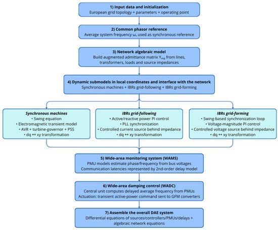
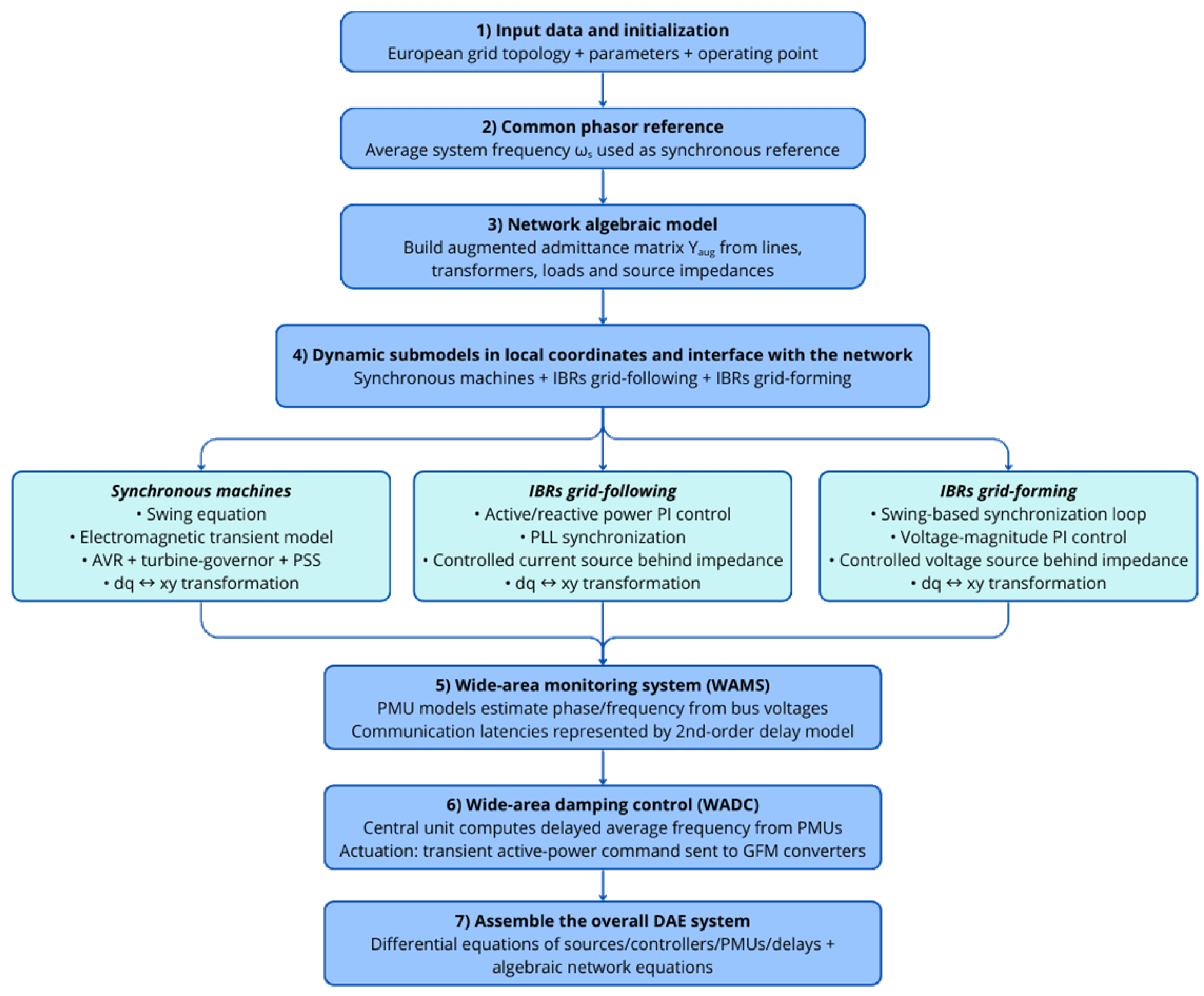
This section presents the mathematical backbone of the overall simulation model. All mathematical models are given in the differential/algebraic equation (DAE) formulation, typically used for power system dynamics [29]. The main references supporting the models can be found in [30,31]. The phasor-based approach has been shown to be suitable for studying slow transients such as in inter-area oscillations and wide-area control applications, even in the presence of inverter-based resources [32]. For the phasor models of all elements, the subscripts xy will denote the rotating coordinates of the system with respect to a common reference frequency, while the subscripts dq will denote the rotating coordinates of the element referenced to its local frequency. The transformations between the coordinate systems will be provided whenever pertinent. The flowchart of the implemented modelling methodology is shown in Figure 1.

Figure 1. Flowchart of the implemented modelling methodology.

3.1. Phasor Reference

The phasor models are formulated with respect to a given reference frequency. This reference frequency for the determination of the angles can be any of the following: a fixed value, typically set to the nominal frequency; the frequency of a selected synchronous machine, usually of relevant rated power; or the centre of inertia of the system [33]. In this work, an alternative reference is proposed and applied. The average frequency of the system is used here as synchronous reference frequency. This approach is preferred to the centre of inertia to reduce the dependence on the knowledge of the inertia of all individual elements while still providing a robust and effective mathematical reference, thus also allowing the inclusion of frequency measurements from PMUs for a more comprehensive determination. The reference ${\omega }_s$ is then given by

$${\omega }_s={\displaystyle \frac{1}{N}}\sum _{i=1}^N{\omega }_i$$

(1)

where N is the number of dynamic elements contributing to the determination of the reference, while ${\omega }_i$ is the frequency of the given dynamic element. In (1), the angular frequency $\omega$ is used instead of the frequency f for consistency with the formulation of the elements models, as shown in the next sections. When working in per-unit values, angular frequency and frequency numerically coincide.

3.2. Network

The overall model of the system is represented in a common rotating xy coordinate system. The network is represented with the nodal equations, which, in matrix, form read as follows:

$${\mathbf{I}}_{inj,x}+j{\mathbf{I}}_{inj,y}=\left({\mathbf{G}}_{aug}+j{\mathbf{B}}_{aug}\right)\left({\mathbf{V}}_x+j{\mathbf{V}}_y\right)$$

(2)

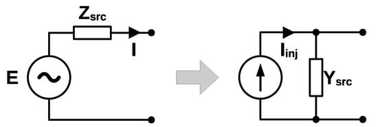
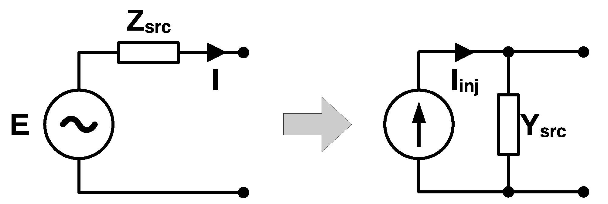
The currents ${\mathbf{I}}_{inj,x}+j{\mathbf{I}}_{inj,y}$ correspond to the currents injected by the active sources. In this work, active sources are synchronous machines and inverter-based resources. The sources are represented as voltages behind impedances. For implementation in the software environment, it is convenient to consider the Norton equivalent of the sources, as shown in Figure 2.

Figure 2. Norton-equivalent implementation of generation sources.

The internal voltage E is determined according to the specific model of the different sources, as described in the next subsections. The generated current $I_x+j{I}_y$ is determined for internal use within the element model if necessary. The injected current $I_{inj,x}+j{I}_{inj,y}$ is instead determined as $\left(E_x+j{E}_y\right)/\left(R_{src}+j{X}_{src}\right)$ to interface with the network equations. The matrix ${\mathbf{G}}_{aug}+j{\mathbf{B}}_{aug}$ is the augmented admittance matrix of the system. This matrix is formed by adding the single admittances of the generation sources to the diagonal of the admittance matrix $\mathbf{G}+j\mathbf{B}$ formed by lines, transformers and constant loads. The determination of the admittance matrix $\mathbf{G}+j\mathbf{B}$ will be presented in the next sections.

The matrix ${\mathbf{G}}_{aug}+j{\mathbf{B}}_{aug}$ is then reduced to the active nodes, where a current injection is present. The reduced matrix is computed as

$${\widehat{\mathbf{Y}}}_{red}={\widehat{\mathbf{Y}}}_{rr}-{\widehat{\mathbf{Y}}}_{re}{\widehat{\mathbf{Y}}}_{ee}^{-1}{\widehat{\mathbf{Y}}}_{er}$$

(3)

where the hat symbol denotes complex quantities, while the subscripts r and e denote the retained and eliminated nodes, respectively. The sub-matrices in (3) correspond to partitions of the augmented admittance matrix. This reduction corresponds to the calculation of the Schur complement of the matrix, and it exploits the condition of zero net injected currents at the eliminated nodes. The voltages ${\widehat{\mathbf{V}}}_r$ of the retained nodes with active generation sources are then computed as ${\widehat{\mathbf{Z}}}_{red}{\widehat{\mathbf{I}}}_{inj}$, with ${\widehat{\mathbf{Z}}}_{red}={\widehat{\mathbf{Y}}}_{red}^{-1}$. The voltages ${\widehat{\mathbf{V}}}_e$ of the eliminated nodes can be calculated as $-{\widehat{\mathbf{Y}}}_{ee}^{-1}{\widehat{\mathbf{Y}}}_{er}{\widehat{\mathbf{V}}}_r$.

3.3. Synchronous Machines

Synchronous machines are represented with a conventional two-axis transient model [34].

The mechanical behaviour of the machine is described by the following swing equations:

$$\begin{array}{cc}\hfill \dot{\delta }& ={\omega }_n\left(\Delta \omega -\Delta {\omega }_s\right)\hfill \end{array}$$

(4)

$$\begin{array}{cc}\hfill 2H\Delta \dot{\omega }& =P_m-P_e-D\Delta \omega \hfill \end{array}$$

(5)

$$\begin{array}{cc}\hfill P_e& =V_q{I}_q+V_d{I}_d\hfill \end{array}$$

(6)

where $\delta$ is the rotor angle, $\Delta \omega$ is the angular speed variation with respect to the nominal speed 1 pu, $P_m$ is the mechanical power, and $P_e$ is the electrical power. The parameter ${\omega }_n$ is the rated angular speed; H is the inertia constant; and D is the friction factor. In (4), ${\omega }_s$ is the common synchronous frequency reference for the system, assigned as discussed in Section 3.1. The variation $\Delta {\omega }_s={\omega }_s-1$ with respect to the nominal 1 pu is considered for modelling convenience.

The electromagnetic behaviour of the machine is described by the following equations:

$$\begin{array}{cc}\hfill T_{d0}^{\prime }{\dot{E}}_q^{\prime }& =-E_q^{\prime }+(X_d-X_d^{\prime })I_d+E_{fd}\hfill \end{array}$$

(7)

$$\begin{array}{cc}\hfill T_{q0}^{\prime }{\dot{E}}_d^{\prime }& =-E_d^{\prime }-(X_q-X_q^{\prime })I_q\hfill \end{array}$$

(8)

where $E_q^{\prime }$ is the transient electromagnetic force due to field flux linkages, $E_d^{\prime }$ is the transient electromagnetic force due to flux linkage in the q-axis damper winding, and $E_{fd}$ is the field excitation voltage. The parameters $X_d$, $X_d^{\prime }$, $X_q$ and $X_q^{\prime }$ are the synchronous and transient reactances along the d-axis and q-axis, respectively; $T_{d0}^{\prime }$ and $T_{q0}^{\prime }$ are the d-axis and q-axis open-circuit transient time constants, respectively. The internal voltage $E_{int,q}^{\prime }+j{E}_{int,d}^{\prime }$ is therefore given by

$$E_{int,q}^{\prime }+j{E}_{int,d}^{\prime }=E_q^{\prime }+j\left[E_d^{\prime }-\left(X_d^{\prime }-X_q^{\prime }\right)I_q\right]$$

(9)

setting the voltage behind the impedance $R_a+j{X}_d^{\prime }$ of the machine. The parameter $R_a$ is the armature resistance.

In (5) and (7), the variables $P_m$ and $E_{fd}$ are input provided by the turbine-governor system and the automatic voltage regulator, respectively.

The current $I_q+j{I}_d$ is obtained with the following equation:

$$I_q+j{I}_d={\displaystyle \frac{E_{int,q}^{\prime }+j{E}_{int,d}^{\prime }-\left(V_q+j{V}_d\right)}{R_a+j{X}_d^{\prime }}}$$

(10)

The injected current is then obtained as

$$I_{inj,q}+j{I}_{inj,d}={\displaystyle \frac{E_{int,q}^{\prime }+j{E}_{int,d}^{\prime }}{R_a+j{X}_d^{\prime }}}$$

(11)

A generic variable $\chi$ of the model (either voltage or current) can be then transformed from the rotating dq coordinates of the machine to the common rotating xy coordinates of the system and vice versa with the following equations:

$$\begin{array}{cc}\hfill {\chi }_x+j{\chi }_y& =\left({\chi }_q+j{\chi }_d\right)e^{j\delta }\hfill \end{array}$$

(12)

$$\begin{array}{cc}\hfill {\chi }_q+j{\chi }_d& =\left({\chi }_x+j{\chi }_y\right)e^{-j\delta }\hfill \end{array}$$

(13)

with anticlockwise and clockwise complex rotations, using the rotor angle $\delta$ of the machine.

It is important to notice that the implemented model of the synchronous machines follows the q-axis alignment for the coordinate transformations and the load convention for the sign of the currents. The models of the primary controllers of the machines are derived from [35] and are described in the next subsections.

3.3.1. Automatic Voltage Regulator

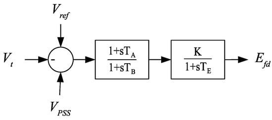
The model of the implemented automatic voltage regulator is described by the following equations:

$$\begin{array}{cc}\hfill T_B{\dot{x}}_f& =-x_f+u\hfill \end{array}$$

(14)

$$\begin{array}{cc}\hfill y_f& =\left(1-{\displaystyle \frac{T_A}{T_B}}\right)x_f+{\displaystyle \frac{T_A}{T_B}}u\hfill \end{array}$$

(15)

$$\begin{array}{cc}\hfill T_E{\dot{E}}_{fd}& =-E_{fd}+K{y}_f\hfill \end{array}$$

(16)

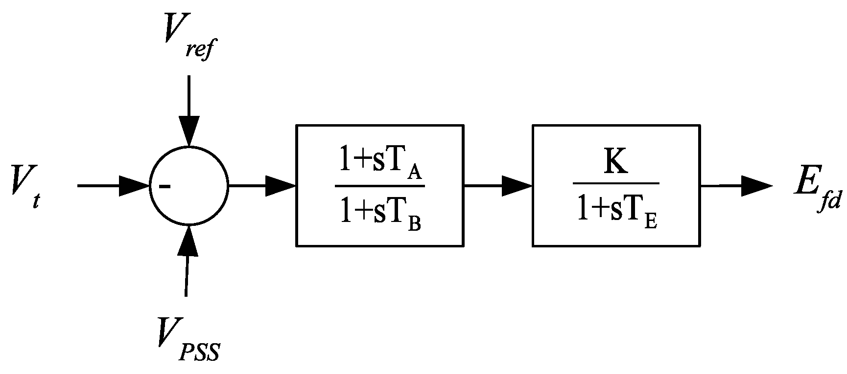
where (14) and (15) implement the lead–lag block of transient gain reduction, while (16) implements the lag block of an amplifier with regulator gain K and time constant $T_E$. The input u is given by $V_{ref}-V_t-V_{PSS}$, where $V_{ref}$ is a constant, $V_t$ is the magnitude of the voltage at the machine terminal, and $V_{PSS}$ is the auxiliary local signal provided by the PSS. For convenience, a block diagram of the automatic voltage regulator is presented in Figure 3.

Figure 3. Block diagram of the automatic voltage regulator.

This specific model of the automatic voltage regulator is considered because it is a standard ENTSO-E controller [35].

3.3.2. Turbine-Governor System

The model of the implemented turbine governor is described by the following equations:

$$\begin{array}{cc}\hfill T_1{\dot{x}}_g& =-x_g+{\displaystyle \frac{1}{R}}\Delta \omega \hfill \end{array}$$

(17)

$$\begin{array}{cc}\hfill T_2{\dot{x}}_t& =-x_t+x_g\hfill \end{array}$$

(18)

$$\begin{array}{cc}\hfill T_m& =\left(1-{\displaystyle \frac{T_1}{T_2}}\right)x_t+{\displaystyle \frac{T_1}{T_2}}{x}_g\hfill \end{array}$$

(19)

where (17) implements the lag block representing the valve, while (18) and (19) implement the lead–lag block representing the reheater. The parameter R is the permanent droop of the regulator. For convenience, a block diagram of the turbine-governor system is presented in Figure 4.

Figure 4. Block diagram of the turbine-governor system.

This specific model of the turbine-governor system is considered because it is a standard ENTSO-E controller [35].

3.3.3. Power System Stabilizer

The model of the implemented power system stabilizer is described by the following equations:

$$\begin{array}{cc}\hfill T_{W1}{\dot{x}}_{w1}& =-x_{w1}+\Delta \omega \hfill \end{array}$$

(20)

$$\begin{array}{cc}\hfill y_{w1}& =-x_{w1}+\Delta \omega \hfill \end{array}$$

(21)

$$\begin{array}{cc}\hfill T_{W2}{\dot{x}}_{w2}& =-x_{w2}+y_{w1}\hfill \end{array}$$

(22)

$$\begin{array}{cc}\hfill y_{w2}& =-x_{w2}+y_{w1}\hfill \end{array}$$

(23)

$$\begin{array}{cc}\hfill T_{W3}{\dot{x}}_{w3}& =-x_{w3}+P_e\hfill \end{array}$$

(24)

$$\begin{array}{cc}\hfill y_{p1}& =-x_{w3}+P_e\hfill \end{array}$$

(25)

$$\begin{array}{cc}\hfill T_7{\dot{x}}_{p2}& =-x_{p2}+K_{S2}{y}_{p1}\hfill \end{array}$$

(26)

$$\begin{array}{cc}\hfill y_{c1}& =y_{w2}+\left(K_{S3}-1\right)x_{p2}\hfill \end{array}$$

(27)

$$\begin{array}{cc}\hfill T_2{\dot{x}}_{c1}& =-x_{c1}+K_{S1}{y}_{c1}\hfill \end{array}$$

(28)

$$\begin{array}{cc}\hfill y_{c2}& =\left(1-{\displaystyle \frac{T_1}{T_2}}\right)x_{c1}+{\displaystyle \frac{T_1}{T_2}}{K}_{S1}{y}_{w2}\hfill \end{array}$$

(29)

$$\begin{array}{cc}\hfill T_4{\dot{x}}_{c2}& =-x_{c2}+y_{c2}\hfill \end{array}$$

(30)

$$\begin{array}{cc}\hfill V_{PSS}& =\left(1-{\displaystyle \frac{T_3}{T_4}}\right)x_{c2}+{\displaystyle \frac{T_3}{T_4}}{y}_{c2}\hfill \end{array}$$

(31)

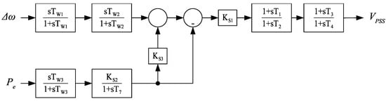
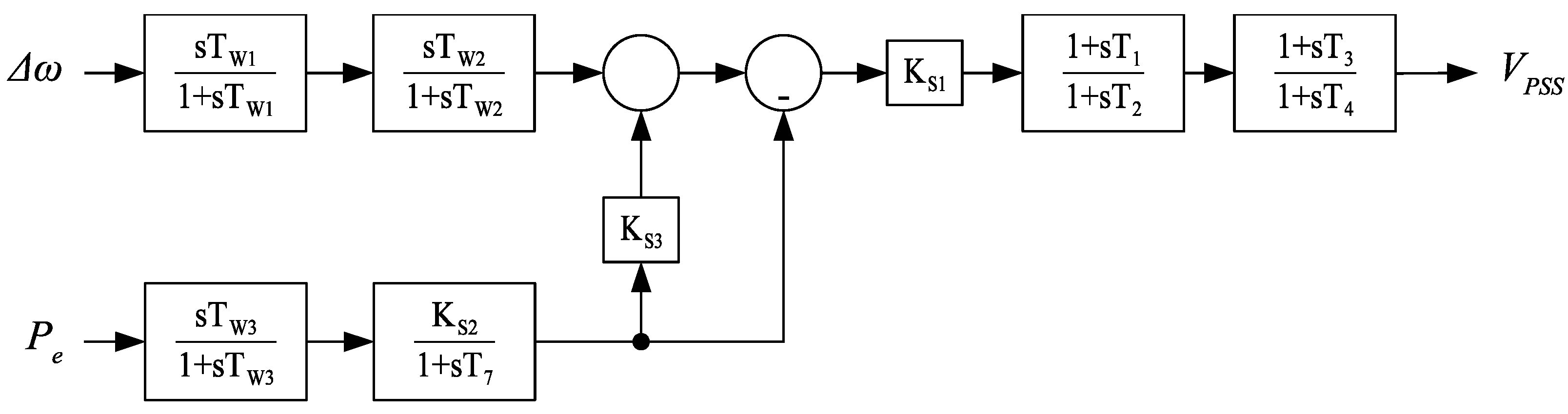
where (20)–(21) and (22)–(23) implement the first and second washout filters on the input variable $\Delta \omega$, respectively; (24)–(25) and (26) implement the washout filter and the low-pass filter on the input variable $P_e$, respectively; (27) combines the control actions on the two input variables; and (28)–(29) and (30)–(31) implement the first and second lead–lag blocks for phase compensation, respectively. For convenience, a block diagram of the power system stabilizer is presented in Figure 5.

Figure 5. Block diagram of the power system stabilizer.

This specific model of the power system stabilizer is considered because it is a standard ENTSO-E controller [35].

3.4. Inverter-Based Resources

Inverter-based resources are represented with a conventional average model [36]. This model uses the average value of the currents and voltages over one switching cycle, effectively modelling the converter as a controlled source. The controlled source is governed by the slower time constants of its outer control loops, which are the loops directly interacting with the time scale of the slow frequency dynamics that are the target of this work.The inverter-based resources are then represented as controlled sources behind a given impedance. The impedance $R_f+j{X}_f$ accounts for the output filter and the coupling transformer of the converter. Depending on the control strategy, the controlled source is a voltage or current source. The implemented control strategies are typical schemes of grid-forming and grid-following converters, as described in the next subsections.

3.4.1. Grid-Forming

The model of the implemented grid-forming control system represents the main outer loops of the control, which are the angle and voltage magnitude control loops. The considered model corresponds to a typical swing-based virtual synchronous machine [37]. The control of the angle is the synchronization loop of the converter, and it is implemented according to the following equations:

$$\begin{array}{cc}\hfill \dot{\delta }& ={\omega }_n\left(\Delta \omega -\Delta {\omega }_s\right)\hfill \end{array}$$

(32)

$$\begin{array}{cc}\hfill K_i\Delta \dot{\omega }& =P_{ref}-P-K_f\Delta \omega \hfill \end{array}$$

(33)

$$\begin{array}{cc}\hfill P& =V_d{I}_d+V_q{I}_q\hfill \end{array}$$

(34)

where $\delta$ is the synchronization angle, $\Delta \omega$ is the frequency variation with respect to the nominal frequency 1 pu, and P is the measured active power. The parameter $P_{ref}$ is the set point for the active power; ${\omega }_n$ is the rated angular speed; $K_i$ is the gain for the emulation of inertia; $K_f$ is the gain for the frequency droop. In (32), $\Delta {\omega }_s$ is the variation of the common synchronous frequency reference (see Section 3.1) with respect to the nominal 1 pu value. The control of the voltage magnitude is implemented according to the following equations:

$$\begin{array}{cc}\hfill {\dot{x}}_V& =K_{Vi}u\hfill \end{array}$$

(35)

$$\begin{array}{cc}\hfill E_{ctrl}& =K_{Vp}u+x_V\hfill \end{array}$$

(36)

where the input u is given by the difference between the voltage set point $V_{ref}$ and the measured voltage V at the converter terminal. The parameters $K_{Vp}$ and $K_{Vi}$ are the proportional and integral gains of the control, respectively. The internal voltage of the controlled source is therefore given by

$$E_d+j{E}_q=E_{ctrl}+j0$$

(37)

The injected current is obtained with the following equation:

$$I_{inj,d}+j{I}_{inj,q}={\displaystyle \frac{E_d+j{E}_q}{R_f+j{X}_f}}$$

(38)

The current $I_d+j{I}_q$ is finally obtained as

$$I_d+j{I}_q={\displaystyle \frac{E_d+j{E}_q-\left(V_d+j{V}_q\right)}{R_f+j{X}_f}}$$

(39)

A generic variable $\chi$ of the model (either voltage or current) can be then transformed from the rotating dq coordinates of the converter to the common rotating xy coordinates of the system and vice versa with the following equations:

$$\begin{array}{cc}\hfill {\chi }_x+j{\chi }_y& =\left({\chi }_d+j{\chi }_q\right)e^{j\delta }\hfill \end{array}$$

(40)

$$\begin{array}{cc}\hfill {\chi }_d+j{\chi }_q& =\left({\chi }_x+j{\chi }_y\right)e^{-j\delta }\hfill \end{array}$$

(41)

with anticlockwise and clockwise complex rotations, using the synchronizing angle $\delta$ of the converter.

3.4.2. Grid-Following

The model of the implemented grid-following control system represents the main outer loops, which are the active power and the reactive power control loops. The model also includes the synchronization loop with a phase-locked loop (PLL) block. The active power control loop is implemented according to the following equations:

$$\begin{array}{cc}\hfill {\dot{x}}_P& =K_{Pi}u\hfill \end{array}$$

(42)

$$\begin{array}{cc}\hfill I_{ctrl,d}& =K_{Pp}u+x_P\hfill \end{array}$$

(43)

where the input u is given by the difference between the power set point $P_{ref}$ and the measured power P at the converter terminal. The parameters $K_{Pp}$ and $K_{Pi}$ are the proportional and integral gains of the control, respectively. The reactive power control loop is implemented according to similar equations:

$$\begin{array}{cc}\hfill {\dot{x}}_Q& =K_{Qi}u\hfill \end{array}$$

(44)

$$\begin{array}{cc}\hfill I_{ctrl,q}& =K_{Qp}u+x_Q\hfill \end{array}$$

(45)

where the input u is given by the difference between the power set point $Q_{ref}$ and the measured power Q at the converter terminal. The parameters $K_{Qp}$ and $K_{Qi}$ are the proportional and integral gains of the control, respectively. The PLL is implemented according to the following equations:

$$\begin{array}{cc}\hfill {\dot{x}}_{\omega }& =K_{PLL,i}{V}_q\hfill \end{array}$$

(46)

$$\begin{array}{cc}\hfill \Delta \omega & =K_{PLL,p}{V}_q+x_{\omega }\hfill \end{array}$$

(47)

$$\begin{array}{cc}\hfill \dot{\delta }& ={\omega }_n\left(\Delta \omega -\Delta {\omega }_s\right)\hfill \end{array}$$

(48)

where $\delta$ is the synchronization angle and $\Delta \omega$ is the frequency variation with respect to the nominal frequency of 1 pu. The parameters $K_{PLL,p}$ and $K_{PLL,i}$ are the proportional and integral gains of the loop filter, respectively.

The current $I_d+j{I}_q$ is simply obtained as

$$I_d+j{I}_q=I_{ctrl,d}+j{I}_{ctrl,q}$$

(49)

The internal voltage of the controlled source is determined with the following equation:

$$E_d+j{E}_q=V_d+j{V}_q+\left(I_d+j{I}_q\right)\left(R_f+j{X}_f\right)$$

(50)

The injected current is then obtained as

$$I_{inj,d}+j{I}_{inj,q}={\displaystyle \frac{E_d+j{E}_q}{R_f+j{X}_f}}$$

(51)

A generic variable $\chi$ of the model (either voltage or current) can be then transformed from the rotating dq coordinates of the converter to the common rotating xy coordinates of the system and vice versa with the following equations:

$$\begin{array}{cc}\hfill {\chi }_x+j{\chi }_y& =\left({\chi }_d+j{\chi }_q\right)e^{j\delta }\hfill \end{array}$$

(52)

$$\begin{array}{cc}\hfill {\chi }_d+j{\chi }_q& =\left({\chi }_x+j{\chi }_y\right)e^{-j\delta }\hfill \end{array}$$

(53)

with anticlockwise and clockwise complex rotations using the synchronizing angle $\delta$ of the converter.

3.5. Lines, Transformers and Loads

Lines and transformers are represented with two-port models, described by the following equations:

$$\begin{array}{cc}\hfill I_{x1}+j{I}_{y1}=& \left(G_{11}+j{B}_{11}\right)\left(V_{x1}+j{V}_{y1}\right)\hfill \\ \hfill +& \left(G_{12}+j{B}_{12}\right)\left(V_{x2}+j{V}_{y2}\right)\hfill \end{array}$$

(54)

$$\begin{array}{cc}\hfill I_{x2}+j{I}_{y2}=& \left(G_{21}+j{B}_{21}\right)\left(V_{x1}+j{V}_{y1}\right)\hfill \\ \hfill +& \left(G_{22}+j{B}_{22}\right)\left(V_{x2}+j{V}_{y2}\right)\hfill \end{array}$$

(55)

where G and B are the real and imaginary parts of the complex admittances, respectively. For a line represented with resistance R and reactance X, the longitudinal admittance ${\widehat{Y}}_{li}$ of the line is $1/(R+jX)$, and the four parameters are given by $G_{11}=\Re \left({\widehat{Y}}_{li}\right)$ and $B_{11}=\Im \left({\widehat{Y}}_{li}\right)$, $G_{12}=G_{21}=\Re (-{\widehat{Y}}_{li})$ and $B_{12}=B_{21}=\Im (-{\widehat{Y}}_{li})$, $G_{22}=\Re \left({\widehat{Y}}_{li}\right)$ and $B_{22}=\Im \left({\widehat{Y}}_{li}\right)$. For transformers, tap positions are not considered because the input data in [14] do not include them. However, when tap positions are available, their consideration in the mathematical formulation of (54) and (55) is straightforward.

Loads are represented in the model as constant shunt admittances, described by the following equation:

$$I_x+j{I}_y=\left(G_{lo}+j{B}_{lo}\right)\left(V_x+j{V}_y\right)$$

(56)

where $G_{lo}+j{B}_{lo}$ is the complex admittance given by $(P_{lo}+j{Q}_{lo})/V_0^2$, considering the active $P_{lo}$ and reactive $Q_{lo}$ power of the load and the initial value $V_0$ of the voltage.

3.6. Phasor Measurement Units

The PMUs are included in the model with the representation of the key PLL-based component. The model measures the frequency and phase of the complex input voltage in the xy coordinates of the system. Assuming that $V_x+j{V}_y$ is the voltage of the node, the PMU is described by the following equations:

$$\begin{array}{cc}\hfill V_q& =-V_{x}sin\left(\delta \right)+V_{y}cos\left(\delta \right)\hfill \end{array}$$

(57)

$$\begin{array}{cc}\hfill {\dot{x}}_{\omega }& =K_{PLL,i}{V}_q\hfill \end{array}$$

(58)

$$\begin{array}{cc}\hfill \dot{\delta }& ={\omega }_n\left(\Delta \omega -\Delta {\omega }_s\right)\hfill \end{array}$$

(59)

$$\begin{array}{cc}\hfill \Delta \omega & =K_{PLL,p}{V}_q+x_{\omega }\hfill \end{array}$$

(60)

where $K_{PLL,p}$ and $K_{PLL,i}$ are the proportional and integral gain of the loop filter, respectively. The frequency $\omega$ is then given per unit by $\Delta \omega +1$. Since the PMU ultimately tracks the frequency of the phasors, the model also accounts for the reference frequency ${\omega }_s$ of the overall mathematical system, as described in Section 3.1.

3.7. Wide-Area Communication System

The communication system is represented with appropriate models of latencies. For power system simulations, the time delays can be modelled with Padé approximants [38]. Here, a rational transfer function strictly of the second order will be taken into consideration. In the time domain, the model of the communication latency is therefore described by the following equations:

$$\begin{array}{cc}\hfill {\dot{x}}_1& =-{\displaystyle \frac{4}{T_d}}{x}_1-{\displaystyle \frac{6}{T_d^2}}{x}_2+u\hfill \end{array}$$

(61)

$$\begin{array}{cc}\hfill {\dot{x}}_2& =x_1\hfill \end{array}$$

(62)

$$\begin{array}{cc}\hfill u_d& =-{\displaystyle \frac{2}{T_d}}{x}_1+{\displaystyle \frac{6}{T_d^2}}{x}_2\hfill \end{array}$$

(63)

where u is the input variable of the delay model, $u_d$ is the delayed variable. The parameter $T_d$ is the time delay.

3.8. Wide-Area Damping Control

The wide-area damping control considered in this work relies on the average frequency of the system as a global feedback signal. This concept was originally introduced in [39,40]. The feedback signal is computed as average of all collected PMU measurements:

$${\omega }_{avg}\left(t\right)={\displaystyle \frac{1}{N}}\sum _i^N{\omega }_{PMU,i}\left(t-T_{di}\right)$$

(64)

The feedback signal ${\omega }_{avg}$ is then sent to the actuators of the wide-area control scheme. The actuation is implemented in the form of transient active power injections:

$$\Delta P_w\left(t\right)=K_w\left[{\omega }_{avg}\left(t-T_d\right)-\omega \left(t\right)\right]$$

(65)

where $\omega$ is the local frequency at the terminal of the actuator. The parameter $K_w$ is a proportional gain to determine the intensity of the control. In this work, the actuators are the grid-forming converters operating in the system. In (64) and (65), the dependence on time has been made explicit, thus denoting the inclusion of the latencies in the model. The round-trip delay will be given by the sum of the latencies in delivering the frequencies ${\omega }_{PMU}$ to the central unit and the latencies in delivering the global feedback signal ${\omega }_{avg}$ to the local actuators.

4. Model Implementation

This sections describes the main features underlying the implementation of the model in the MATLAB/Simulink software (version 2024b). Even if the model is made openly available, this description allows comprehensive insight, fostering model transparency and simulation replicability.

4.1. MATLAB/Simulink Features

The development of the model in the MATLAB/Simulink environment starts from the implementation principles reported in [41] for the benchmark IEEE 68-bus system. Fundamental modifications and extensions are made.

In the model designed for the benchmark system, the synchronous machines must be strictly connected to the first nodes in numeric order, and unit transformation matrices are used for the construction of the voltages and currents. In this work, the model is modified by introducing arrays of indexes, removing the limitation of the rigid progressive order of generation nodes. Using Assignment and Selector blocks, this approach eliminates the need of transformation matrices, thus allowing a completely general interface between active sources and network equations. Another important modification concerns the implementation of the admittance matrix. While, in the model designed for the benchmark system, the full admittance matrix is considered and inverted, the Simulink model implemented in this work relies on a computational efficient approach based on the Schur complement.

The parameters of the model are loaded and assigned through the initial execution of a MATLAB script. In the script, the initialization of the state variables is also performed. A given power flow solution for the European power system is considered. Different power flow conditions can be considered without any loss of generality. The starting dataset in [14] does not include any inverter-based resources. The addition of grid-forming and grid-following converters is performed assuming an arbitrary integration case, with a random assignment of the converter-based generation sources. It is worth noting that numbers and distribution of IBRs in the system have been determined exclusively to demonstrate possible generic usages of the WAMCES model with integration of IBRs, without any claim of realistic operating conditions of the system. The developed WAMCES model is then capable of considering new forms and features of the modern power systems, such as the penetration of power electronics and the distribution of advanced measurement devices.

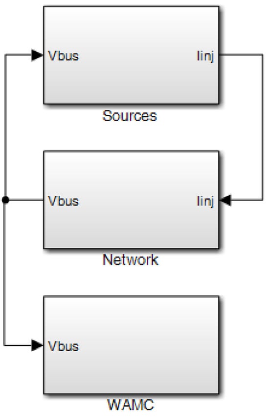
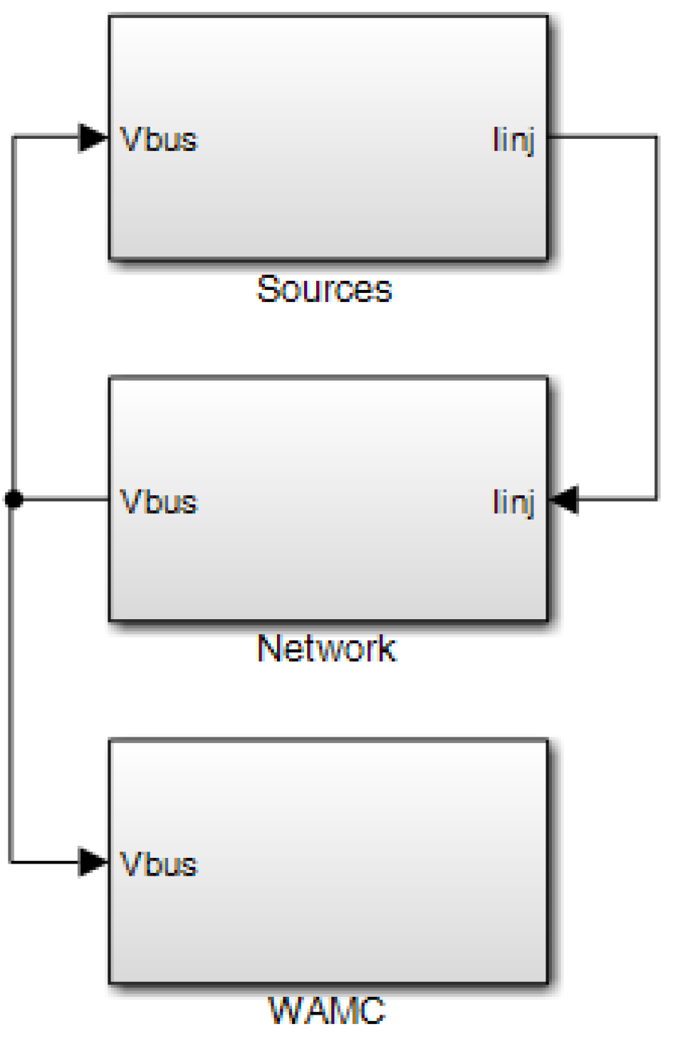
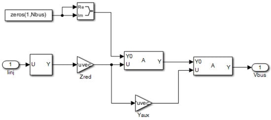
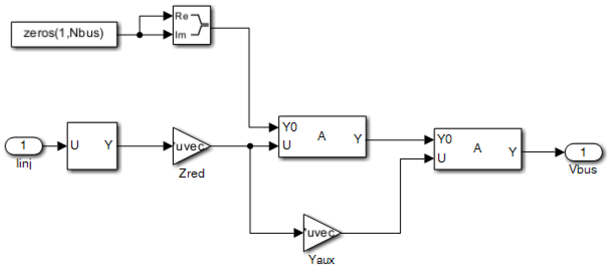
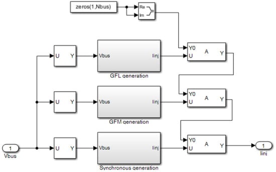
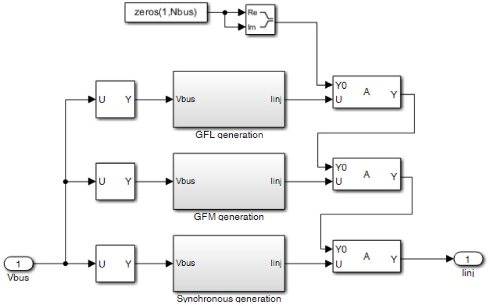
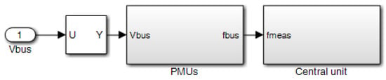
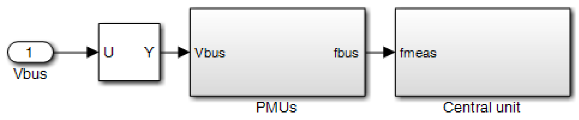
The final model relies on vectorized operations, as allowed by the features of MATLAB/Simulink. When necessary, elementwise operations with dot punctuation $.\setminus$ and $.\ast$ are performed. This guarantees compact model implementation. The top-level diagram of the MATLAB/Simulink model is shown in Figure 6. The model is organized in three main subsystems. The subsystem `Network’ is detailed in Figure 7 and implements the algebraic equations as described in Section 3. Figure 8 shows the subsystem ‘Sources’, where the three main types of synchronous generation as well as IBR grid-following and IBR grid-forming are grouped in the corresponding subsystems. The subsystem ‘WAMC’ implements the wide-area monitoring and control features, as shown in Figure 9. According to the mathematical formulation of Section 3, the wide-area monitoring system is represented with PMUs and communication delays, while the wide-area damping control is implemented by a central computation unit for feedback signal determination and actuation by selected IBR generation sources that receive the reference signal from the central unit. More details about the nested subsystems can be directly found in the model available in [16].

Figure 6. Top-level diagram of the MATLAB/Simulink model implementation.

Figure 7. Subsystem ‘Network’.

Figure 8. Subsystem ‘Sources’.

Figure 9. Subsystem ‘WAMC’.

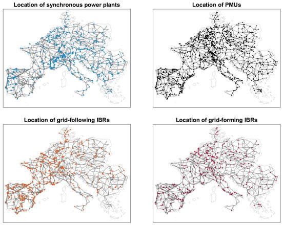
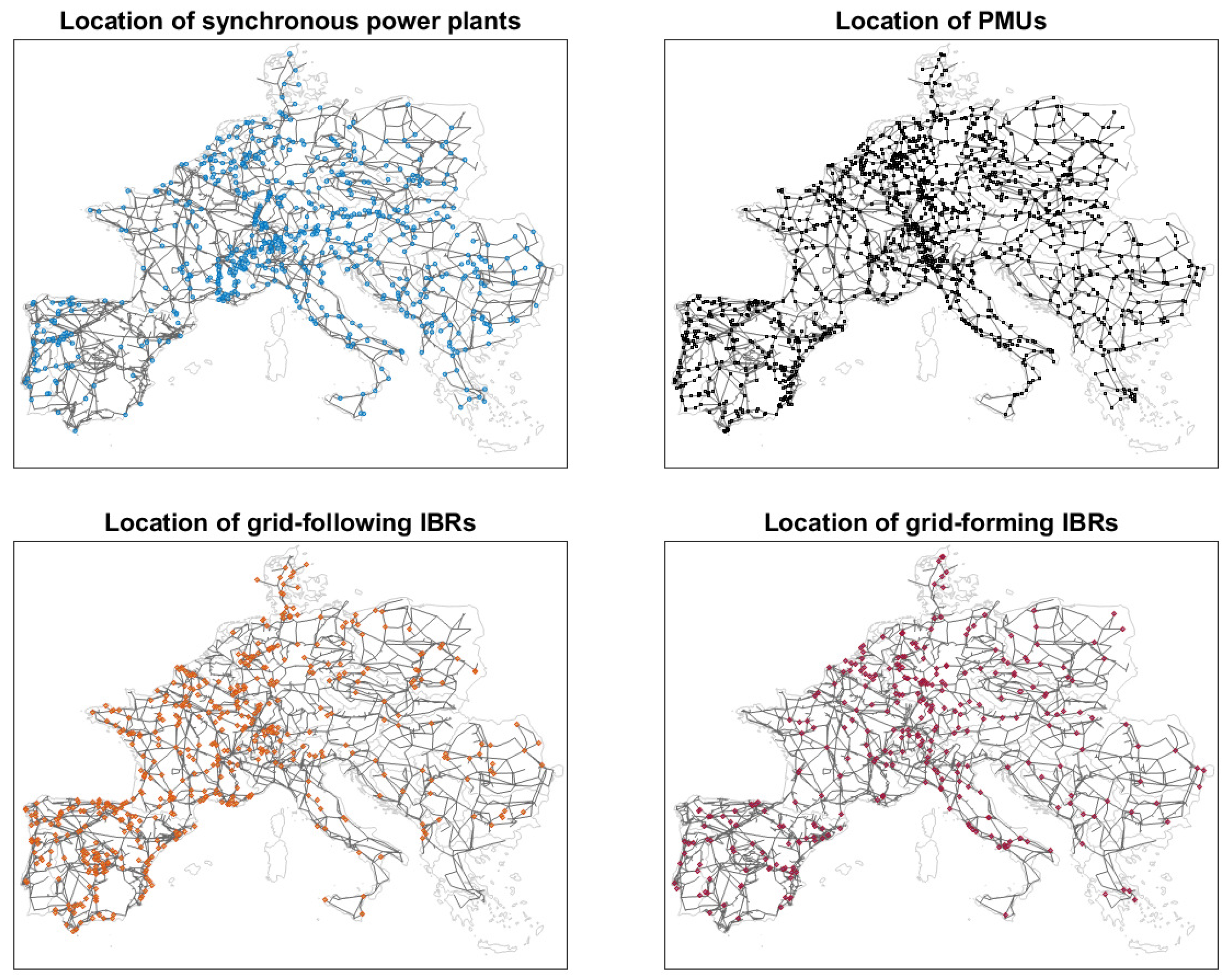
The WAMCES model has 3809 nodes, 7343 branches, 618 synchronous machines with 1854 controllers, and 1573 PMUs. The resulting mathematical system has a total number of 20,935 dynamic states. The admittance matrix before Schur reduction has a size of $7618\times 7618$ (complex $3809\times 3809$), while the matrix size after Schur reduction is $2836\times 2836$ (complex $1418\times 1418$).

The outline of the implemented model is reported in Figure 10, where example locations of the main dynamic elements are shown. The structural data of the model are fully available in [16] and are also reported in Appendix A for immediate reference.

Figure 10. Outline of the developed dynamic model of the European power system.

4.2. Model Validation

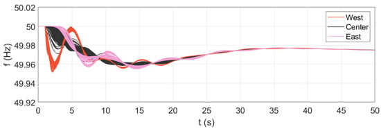
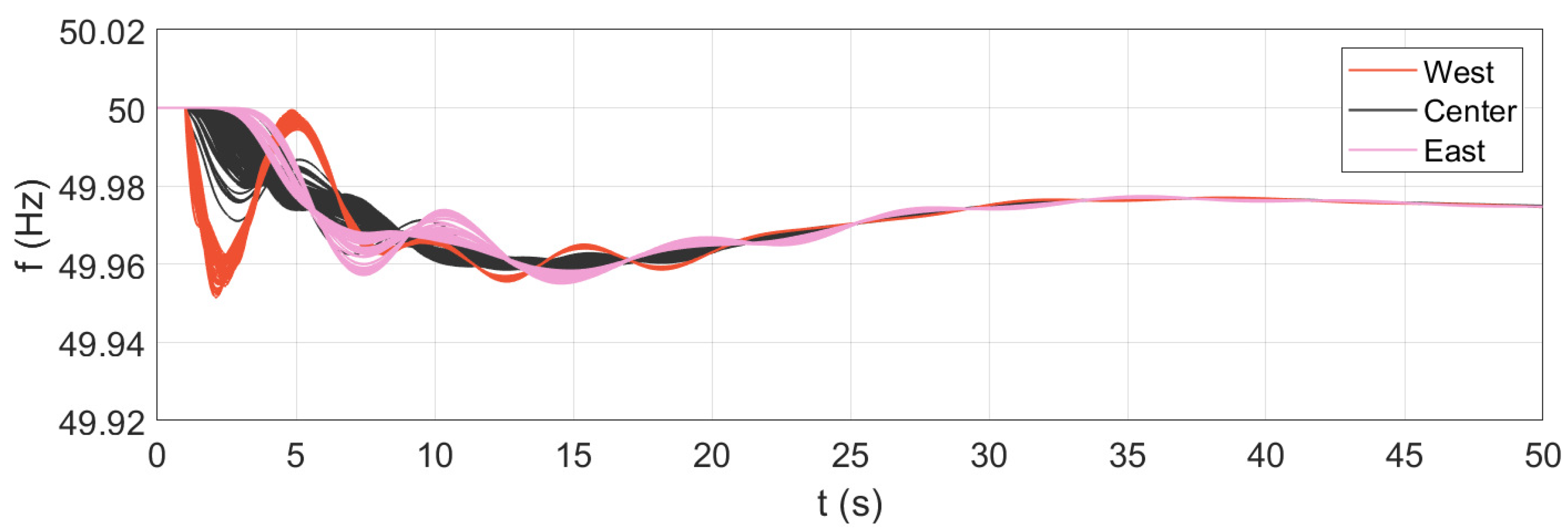
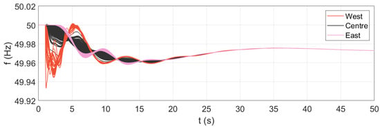
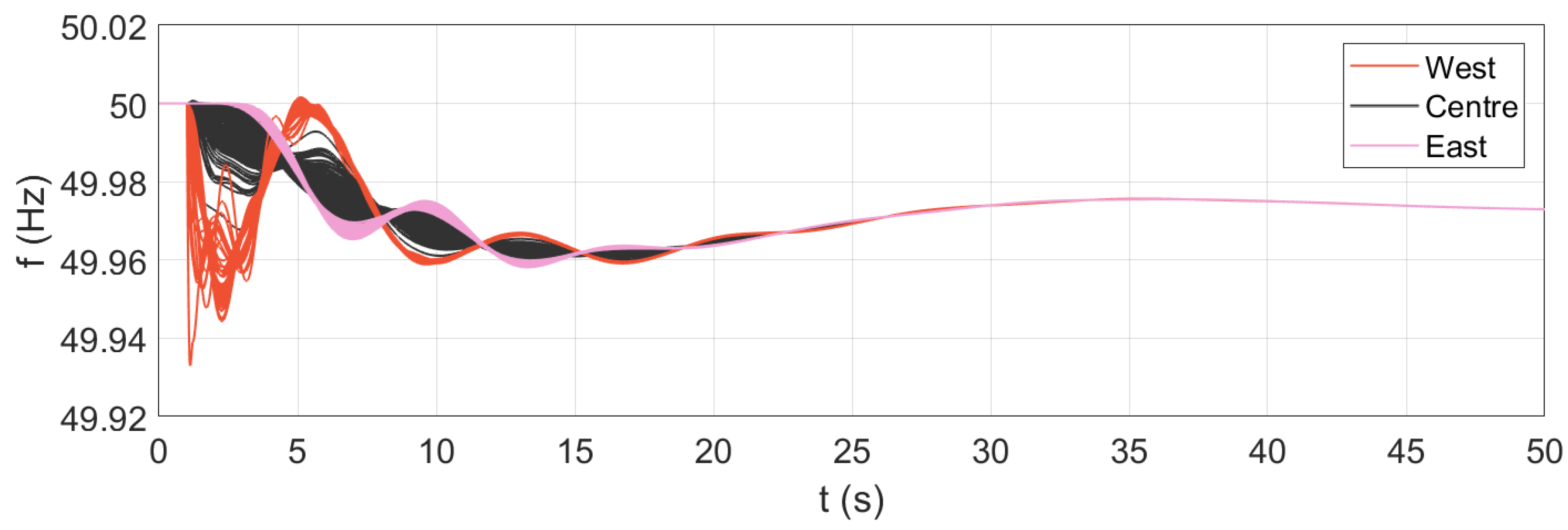
The implemented model is validated, taking the large-scale dynamic model of the ENTSO-E [17] as a reference. As discussed in Section 2, the ENTSO-E model does not include any features related to wide-area monitoring and control applications. For the sake of this comparison, the WAMCES model has been therefore considered under similar assumptions: all features related to wide-area monitoring and control have been deactivated, and only synchronous generation has been included in the system. While the WAMCES model is implemented and simulated in MATLAB/Simulink, the ENTSO-E initial dynamic model is simulated in the specialized power systems software NEPLAN (version V10/360). The comparison between the two models is performed under the assumption of a 1000 MW power imbalance in Western Europe. This disturbance excites the West–East oscillation modes of the European system and corresponds to an actual incident that has been used as validating reference for the ENTSO-E dynamic model itself [18]. The results of the simulation of the two models are shown in Figure 11 and Figure 12, respectively.

Figure 11. Simulation results: ENTSO-E initial dynamic model in NEPLAN.

Figure 12. Simulation results: proposed European dynamic model in MATLAB/Simulink.

The results indicate that the WAMCES model is in close agreement with the ENTSO-E reference. The inter-area oscillations between West and East are clearly visible, with a frequency of around 0.13 Hz, matching the expected modal analysis [17]. Both instantaneous and steady-state frequency deviations substantially match as well, denoting an acceptable agreement for all areas of the system. It is worth noting that, besides the difference of being implemented and simulated in two different simulation tools, the two models of the European power system present some differences, the major ones being the detail of the network representation, the number of synchronous machines and the geographical extension. In this sense, the starting model in [14] has a lower level of detail, covering only 220 kV and 400 kV voltage levels; features a smaller number of synchronous machines; and does not include the Turkish power system area. All these aspects prevent exact alignment between the two models. Nevertheless, the results clearly demonstrate that the WAMCES model is capable of reproducing the essential wide-area dynamics shown by the reference.

For a more comprehensive evaluation of the system performance, a modal analysis is performed for a selected frequency range of interest. The frequency range is selected according to the known inter-area oscillation modes of the European system, as detailed in [17]. The calculations are performed for the following configurations:

• All synchronous generation, no IBRs;
• Integration of IBRs, no wide-area control;
• Integration of IBRs and wide-area control.

The results are given in Table 2, Table 3 and Table 4.

Table 2. Results of the modal analysis in different configurations: East–Centre–West mode.

Configuration	Frequency (Hz)	Damping Ratio (%)
all synchronous generation, no IBRs	0.23	11
integration of IBRs, no WADC	0.22	14
integration of IBRs and WADC	-	-

Table 3. Results of the modal analysis in different scenarios—East–West mode.

Configuration	Frequency (Hz)	Damping Ratio (%)
all synchronous generation, no IBRs	0.13	11
integration of IBRs, no WADC	0.13	20
integration of IBRs and WADC	-	-

Table 4. Results of the modal analysis in different scenarios—North–South Mode.

Configuration	Frequency (Hz)	Damping Ratio (%)
all synchronous generation, no IBRs	0.39	10
integration of IBRs, no WADC	0.38	11
integration of IBRs and WADC	0.31	62

The results immediately show the effectiveness of the applied wide-area control in terms of system damping. The damping ratio is remarkably increased for all the most relevant inter-area oscillation modes of the European system. In particular, for the East–Centre–West mode and the East–West mode, it can be observed that the inter-area oscillations basically disappear from the system, as no oscillation modes are found in the corresponding frequency range. Concerning the North–South mode, an oscillation mode is found even when the wide-area damping control is applied; therefore, inter-area oscillations between those parts of the system are still present. Nevertheless, the damping ratio is significantly improved, increasing sixfold in comparison with the cases where no wide-area control is implemented.

5. Simulations and Results

The application of the presented WAMCES model is demonstrated for different use cases. Specifically, the model is simulated for the following three contingencies:

• Forced oscillations;
• System split;
• Power imbalance.

The rationale for choosing these three cases is the following: the first two cases are examples of wide-area monitoring applications, where the PMUs and the communication system are employed to track frequency oscillations in the system; the last case is instead an example of a wide-area control application, where a central unit computes a global feedback signal and sends it to local IBR actuators in different areas of the system. Given the significant diversity in the nature of the considered contingencies, this ultimately allows a more comprehensive evaluation of the model’s capabilities. For the sake of uniformity, the three contingencies will be applied with a focus on the Iberian peninsula, as described in the next subsections. For a more complete quantification of the numerical results, the energy involved in the system oscillations $E_{osc}$ is considered as a performance metric:

$$E_{osc}=\sum _{i=1}^N\sum _{t=0}^{T_{sim}}|f_{i,t}-f_{avg,t}{|}^2\Delta t$$

(66)

This metric reflects the degree of coherency of the system: small values correspond to good wide-area damping performance, denoting strong coherency of all areas, while high values indicate poor damping properties of the system.

In terms of computational performance, the selected solver is a fixed-step-size ODE3 Bogacki–Shampine, with a sample time of $T_s=0.01$ s. For a simulation time of 50 s, the time required for the execution of the full WAMCES model is approximately 36 s. The calculations are performed on a machine with a 13th Gen Intel(R) Core(TM) i7-1355U 1700 MHz processor and 32.0 GB RAM.

5.1. Forced Oscillations

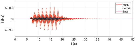
For the application to the use case of forced oscillations, three selected IBR generation sources have been modified to include malfunctioning of the control system, mimicking the source of the considered contingency. The anomaly in the control is replicated by adding to the reference power $P_{ref}$ a transient signal $P_{forced}$, obtained by multiplying the signal $K_{ampl}sin\left(2\pi f_{osc}t\right)$ and an activation signal ramping up from zero to one, remaining at one for a given time and then ramping down back to zero. The parameters of the transient signal determine an oscillation amplitude of 5% ($K_{ampl}=0.05$) and an oscillation frequency of 0.6 Hz ($f_{osc}=0.6$). The three selected sources are nearby IBR power plants located in the Iberian peninsula. This approach triggers forced oscillations in the network, resulting in specific transients in the system. The model also features the inclusion of more than 1500 PMUs and a corresponding communication system for the collection of the measurements. The results of the simulations are reported in Figure 13, showing the frequency measurements acquired by the PMUs and the communication system. From the results, it can be observed that the oscillatory phenomena are captured by the wide-area monitoring feature implemented in the model. The measurements clearly exhibit the 0.6 Hz forced oscillations in the system, also pointing out the occurrence of intra-area oscillations within the Western part of the system.

Figure 13. Simulation results: WAMS during forced oscillations.

5.2. System Split

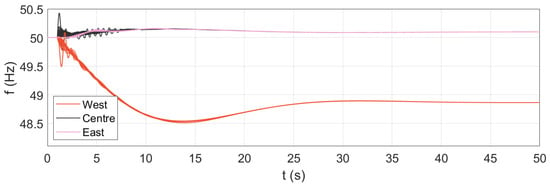
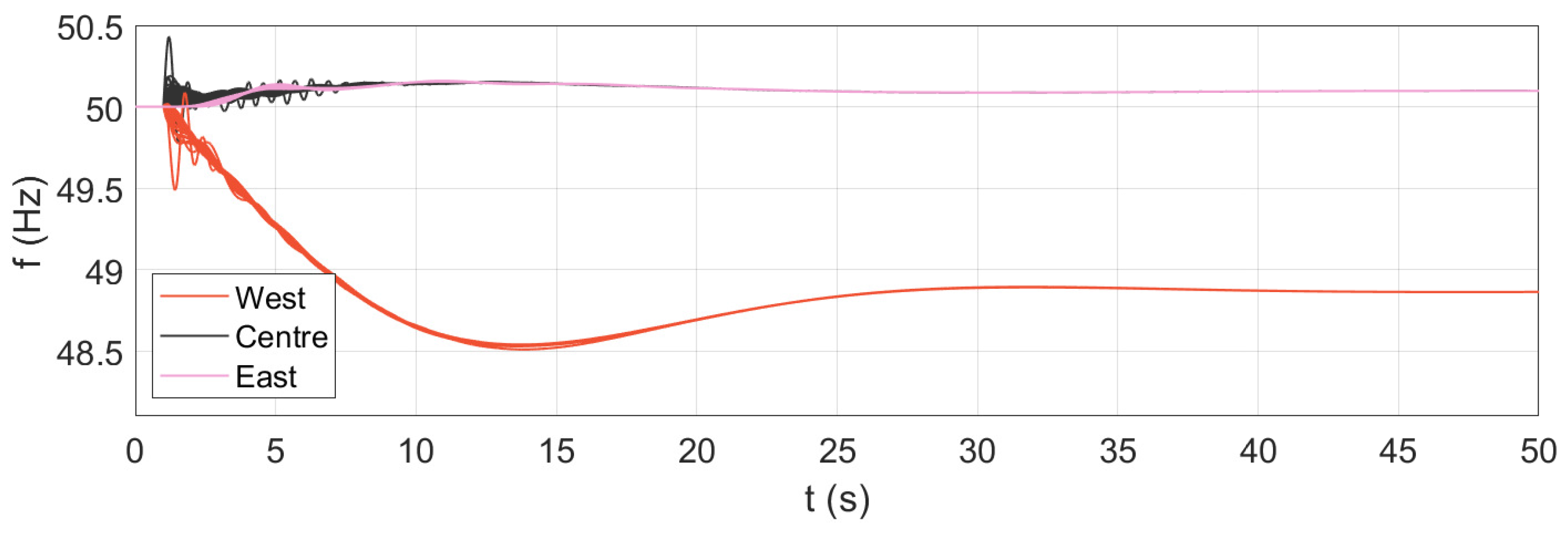
For the application to the use case of a system split, all interconnecting lines between the Iberian peninsula and the remaining part of the continental Europe system are disconnected during the simulation. The selected interconnections include a total of four lines, and the total transfer before the separation is approximately 2.5 GW. The opening of the lines leads, therefore, to a significant frequency transient in both parts of the separated system. Since the system is split into two independent parts, it is expected that smaller area will experience more severe frequency excursions. The results of the simulations are presented in Figure 14, which shows the frequency measurements acquired by the PMUs and the communication system in both parts of the system. The WAMS captures the first oscillations immediately after the system split. Then, the large part of the continental European system experiences a contained overfrequency transient, while the Iberian peninsula undergoes a severe underfrequency transient. It is important to note that this application is taken exclusively as demonstrative example of the WAMCES model in the event of system-split conditions, without the aim of being representative of any specific assessment of the system. In actual operating conditions, underfrequency load shedding and other protective actions would take place, supporting the system during the incident. Although they are outside the scope of this work, these protective actions can be also integrated into the WAMCES model for a more accurate representation of the system’s dynamic response.

Figure 14. Simulation results: WAMS during a system split.

5.3. Power Imbalance

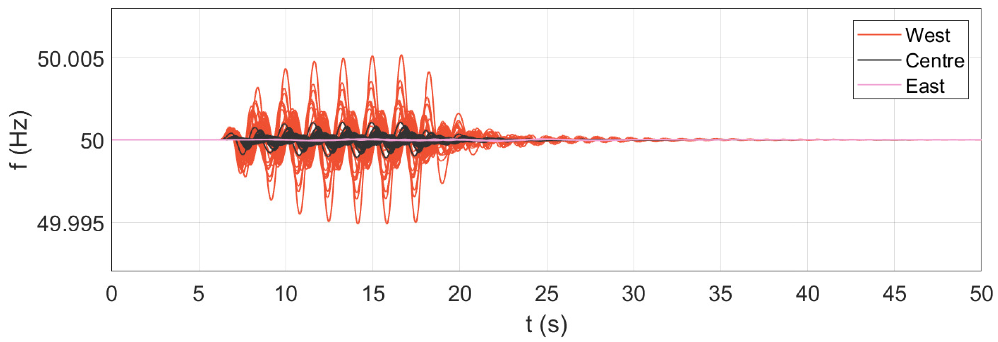
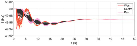
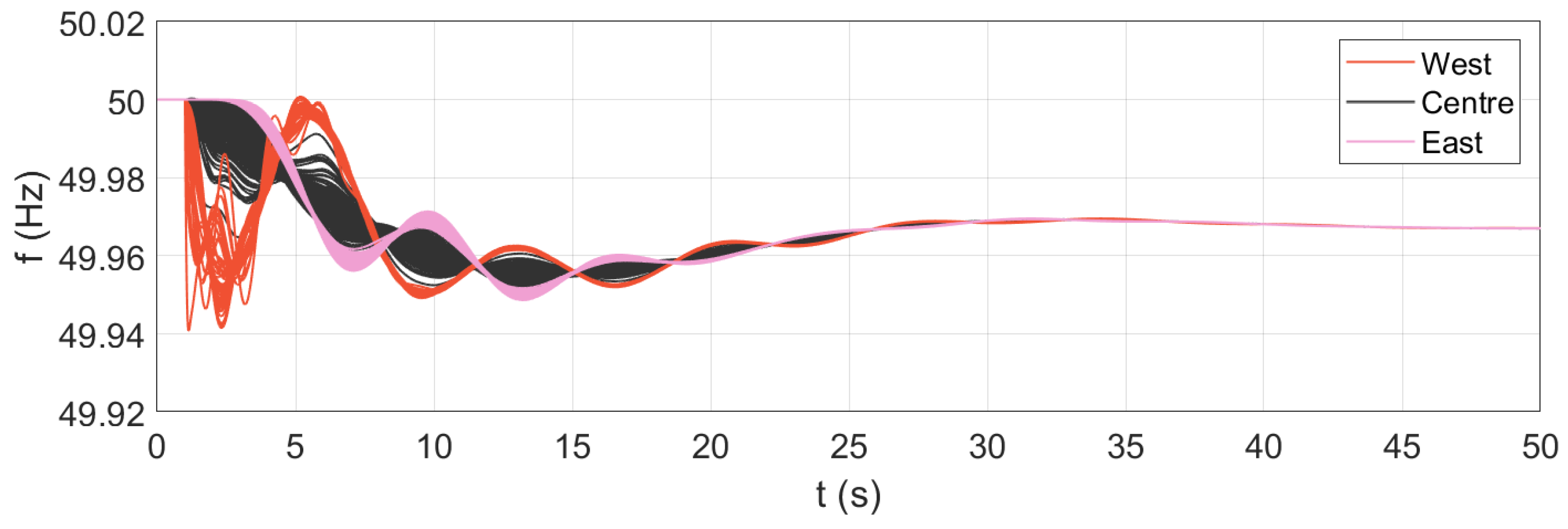
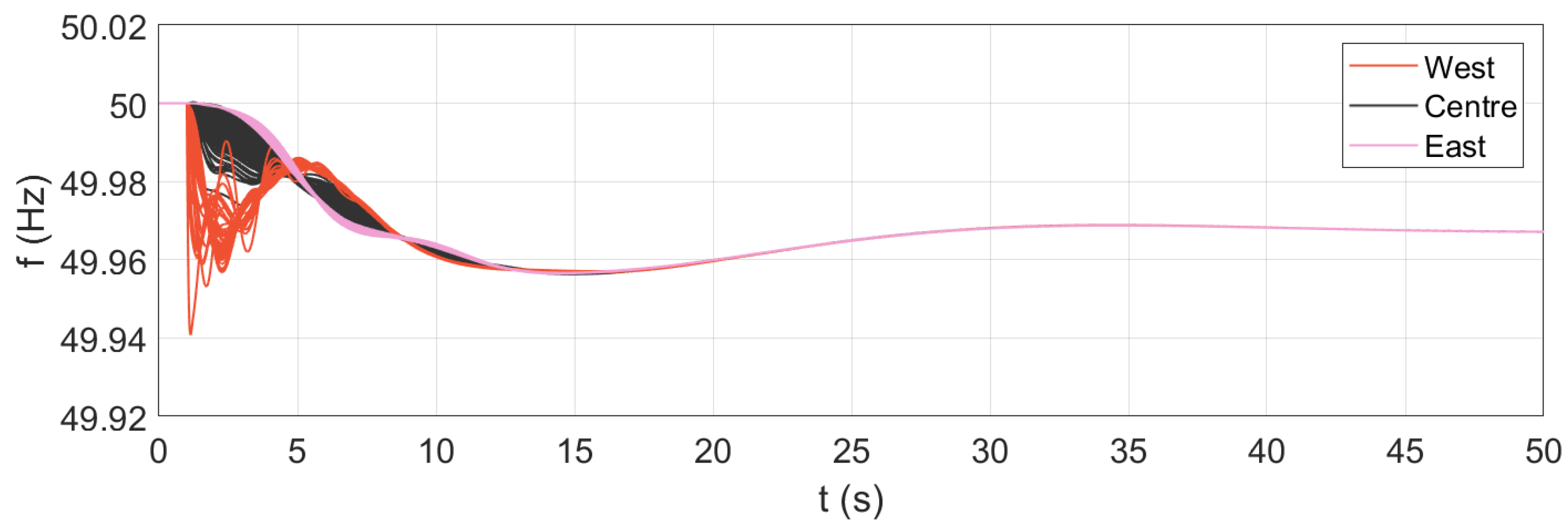
For application to the use case of power imbalance, the model is simulated for a 1 GW generation loss on the Iberian peninsula. This contingency corresponds to the actual disturbance used for the validation of the model, as previously described. In this application example, however, the WAMCES model also includes IBR generation sources and a specific wide-area damping control. The model integrates 300 IBR grid-forming sources and 500 IBR grid-following sources, distributed across all areas of the system. The distribution and integration level of IBR generation sources are determined reasonably yet randomly; they are assumed only for demonstrative purposes of the possible use of the model and do not reflect any actual operating condition of the system. The model also features a wide-area damping control implementation that relies on a central computation unit, a communication system for the exchange of local and global signals, and the actuation in the control system of the IBR grid-forming sources. The results of the simulations are given in terms of recorded frequencies, as shown in Figure 15 for the case without wide-area control and in Figure 16 for the case with wide-area damping control.

Figure 15. Simulation results: IBR integration, no WADC.

Figure 16. Simulation results: IBR integration and WADC.

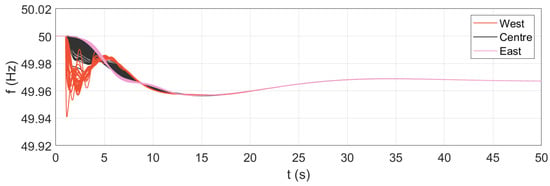
The results show that the considered inclusion of IBR generation sources results in an increase in the amplitude of the oscillations, lasting several seconds after the occurrence of the disturbance (see Figure 12 and Figure 15). The West and East inter-area oscillations are clearly visible, matching the expected low-frequency range. In this case of only IBR integration, the total oscillation energy is equal to $E_{osc}=0.36$ pu·s. The inter-area oscillations exhibit a contained damping ratio, with a decay time of some tens of seconds. With the application of the wide-area damping control, the inter-area oscillations between West and East are notably reduced (Figure 16). By the effect of the IBR actuators that process the global feedback signals provided by the wide-area control central unit, the overall damping capabilities of the European power system are significantly improved. In this case of wide-area control application, the total oscillation energy is equal to $E_{osc}=0.06$ pu·s. This value quantifies the effectiveness of the wide-area damping control application, producing a reduction of about 80% in the energy involved during the system oscillations. The inter-area oscillations exhibit a significant damping ratio, with a decay time of just a few seconds. The results show the positive impact of the applied wide-area damping control on the dynamic response of the system, thus demonstrating a possible use of the WAMCES model for wide-area control applications.

6. Conclusions

The paper presented the development of a large scale dynamic model of the European power system, explicitly designed for wide-area monitoring and control studies. The model includes detailed representations of synchronous machines, inverter-based resources with both grid-forming and grid-following control strategies, and the essential communication and measurement infrastructures. The implementation in MATLAB/Simulink ensures full transparency, flexibility, and computational efficiency, enabling reproducible research and further extensions. Simulation results under different configurations confirmed the ability of the proposed model to accurately capture inter-area oscillation dynamics and evaluate wide-area control strategies. The application of a novel wide-area damping control based on grid-forming converters yielded significant improvements in system damping and overall dynamic performance. The application to different use cases and the numerical results also suggest that the WAMCES model can be useful to system operators for performing analyses in present and future conditions. Although demonstrated only for particular case studies in this work, the model can be generalized to any power system application with proper further development. While implementing all essential features for wide-area monitoring and control applications, the model excludes relevant aspects such as protection modelling for underfrequency load-shedding (UFLS), dynamic modelling of loads for voltage and frequency dependency, voltage regulation in the transmission network with on-load tap changers (OLTC), and implementation of EMT electromagnetic analyses. While these points represent limitations of the model, they simultaneously point out the versatility and the potential of the WAMCES model, since those aspects can be easily added to the model with tailored developments, targeting the specific application and aim of the study. This versatility also makes the WAMCES model suitable for specific studies and investigations such as impact studies of the wide-area geographical distribution of IBRs in the system, sensitivity studies of IBR penetration levels and sensitivity analyses of communication network delays. The developed model, made publicly available, represents a valuable open-access resource for the research community. It provides a solid foundation for further investigations of wide-area control architectures, oscillation damping, and stability enhancement in future power systems with high shares of inverter-based generation.

References

- Benasla, M.; Berkani, A.; Bouchenafa, I.; Allaoui, T.; Korba, P.; Segundo Sevilla, F.R.; Ramirez-Gonzalez, M. Robust Input/Output Signal Selection for WADCs: Comparing Independent and Parallel Operation with Local PSSs. Energies 2026, 19, 954. [Google Scholar] [CrossRef] [Scilit]
- Kwon, K.B.; Ye, L.; Gupta, V.; Zhu, H. Communication-Aware Wide-Area Damping Control Using Risk-Constrained Reinforcement Learning. IEEE Trans. Smart Grid 2026, 17, 678–689. [Google Scholar] [CrossRef] [Scilit]
- Bento, M.E.C. Multi-Objective Approach for Wide-Area Damping Control Design. Symmetry 2025, 17, 1781. [Google Scholar] [CrossRef] [Scilit]
- Zhang, C.; Chang, X.; Dai, J.; Chen, Z.; Babanezhad, M. Designing of a wide-area power system stabilizer using an exponential distribution optimizer and fuzzy controller considering time delays. Sci. Rep. 2025, 15, 1773. [Google Scholar] [CrossRef] [Scilit] [PubMed]
- Musca, R.; Riva Sanseverino, E.; Guerrero, J.M.; Vasquez, J.C. Wide-Area Damping Control for Clustered Microgrids. Energies 2025, 18, 1632. [Google Scholar] [CrossRef] [Scilit]
- Aravena, I.; Sun, C.C.; Shi, R.; Majumder, S.; Yan, W.; Joo, J.Y.; Xie, L.; Wang, J. Open Power System Datasets and Open Simulation Engines: A Survey Toward Machine Learning Applications. IEEE Open Access J. Power Energy 2025, 12, 353–365. [Google Scholar] [CrossRef] [Scilit]
- Ali, A.; Yin, J.; Li, F.F.; Cui, H. Pathway Toward an Open Source Ecosystem in Power Systems: A blueprint for collaborative innovation and software sustainability. IEEE Electrif. Mag. 2025, 13, 58–67. [Google Scholar] [CrossRef] [Scilit]
- Henriquez-Auba, R. Open Source Modeling for Power Systems Dynamics. In Proceedings of the Openmod Meets USA 2023, San Francisco, CA, USA, 13–14 November 2023. [Google Scholar]
- Steiger, T.; John, R. Validation study of an open source extra-high voltage power grid model for Germany. In Proceedings of the 2025 7th Global Power, Energy and Communication Conference (GPECOM), Bochum, Germany, 11–13 June 2025. [Google Scholar]
- Pabón Ospina, L.D.; Lohr, S.; Nuschke, M.; Strauss-Mincu, D.; Bongrain, M.P.; Cossart, Q.; Chiaramello, M. Open-Source Power System Dynamic Models and Test Cases in Modelica: An application example. In Proceedings of the 2023 IEEE PES Innovative Smart Grid Technologies Europe (ISGT EUROPE), Grenoble, France, 23–26 October 2023. [Google Scholar]
- Su, T.; Peng, J.; Selim, A.; Zhao, J.; Tan, J. A Survey of Open-Source Power System Dynamic Simulators with Grid-Forming Inverter for Machine Learning Applications. In Proceedings of the 2025 IEEE Power & Energy Society General Meeting (PESGM), Austin, TX, USA, 27–31 July 2025. [Google Scholar]
- Masoom, A.; Guironnet, A.; Zeghaida, A.; Ould-Bachir, T.; Mahseredjian, J. Modelica-based simulation of electromagnetic transients using Dynaωo: Current status and perspectives. Electr. Power Syst. Res. 2021, 197, 107340. [Google Scholar] [CrossRef] [Scilit]
- Lara, J.D.; Henriquez-Auba, R.; Bossart, M.; Callaway, D.S.; Barrows, C. PowerSimulationsDynamics.jl—An Open Source Modeling Package for Modern Power Systems with Inverter-Based Resources. arXiv 2024, arXiv:2308.02921. [Google Scholar] [CrossRef] [Scilit]
- PanTaGruEl—Open Access Model of the European Transmission Grid. Available online: https://zenodo.org/records/2642175#%20.YdV-M_6ZNPY (accessed on 17 March 2026).
- Pagnier, L.; Jacquod, P. Inertia location and slow network modes determine disturbance propagation in large-scale power grids. PLoS ONE 2019, 14, e0213550. [Google Scholar] [CrossRef] [Scilit] [PubMed]
- WAMCES—Wide-Area and Control of the European Power System. Available online: https://zenodo.org/records/18721887 (accessed on 17 March 2026).
- ENTSO-E SPD (System Protection & Dynamics) Subgroup. Dynamic Model of Continental Europe V2. June 2024. Available online: https://eepublicdownloads.blob.core.windows.net/public-cdn-container/clean-documents/SOC%20documents/Public_report_DYNAMIC_MODEL_OF_CONTINENTAL_EUROPE_V2.pdf (accessed on 17 March 2026).
- Semerow, A.; Höhn, S.; Luther, M.; Sattinger, W.; Abildgaard, H.; Garcia, A.D.; Giannuzzi, G.M. Dynamic Study Model for the Interconnected Power System of Continental Europe in Different Simulation Tools. In Proceedings of the 2015 IEEE Eindhoven PowerTech, Eindhoven, The Netherlands, 29 June–2 July 2015. [Google Scholar]
- ENTSO-E, Initial Dynamic Model of Continental Europe. Available online: https://www.entsoe.eu/publications/system-operations-reports/#entso-e-dynamic-model-of-continental-europe (accessed on 17 March 2026).
- Giannuzzi, G.M.; Lauria, D.; Pisani, C.; Sattinger, W.; Villacci, D. A dynamic equivalencing preliminary study on ENTSO-E CESA power system. In Proceedings of the 2015 AEIT International Annual Conference (AEIT), Naples, Italy, 14–16 October 2015. [Google Scholar]
- Hewes, D.; Altschaeffl, S.; Boiarchuk, I.; Witzmann, R. Development of a Dynamic Model of the European Transmission System using Publicly Available Data. In Proceedings of the 2016 IEEE International Energy Conference (ENERGYCON), Leuven, Belgium, 4–8 April 2016. [Google Scholar]
- Zhou, Q.; Bialek, J.W. Approximate Model of European Interconnected System as a Benchmark System to Study Effects of Cross-Border Trades. IEEE Trans. Power Syst. 2005, 20, 782–788. [Google Scholar] [CrossRef] [Scilit]
- Wang, Y.; Silva, V.; Lopez-Botet-Zulueta, M. Impact of high penetration of variable renewable generation on frequency dynamics in the Continental Europe interconnected system. IET Renew. Power Gener. 2016, 10, 10–16. [Google Scholar] [CrossRef] [Scilit]
- Josz, C.; Fliscounakis, S.; Maeght, J.; Panciatici, P. AC Power Flow Data in MATPOWER and QCQP Format: ITesla, RTE Snapshots, and PEGASE. arXiv 2016, arXiv:1603.01533v3. [Google Scholar] [CrossRef] [Scilit]
- Villella, F.; Leclerc, S.; Erlich, I.; Rapoport, S. PEGASE pan-European test-beds for testing of algorithms on very large scale power systems. In Proceedings of the 2012 3rd IEEE PES Innovative Smart Grid Technologies Europe (ISGT Europe), Berlin, Germany, 14–17 October 2012. [Google Scholar] [CrossRef] [Scilit]
- Zimmerman, R.D.; Murillo-Sanchez, C.E. MATPOWER. 2025. Available online: https://matpower.org (accessed on 17 March 2026).
- Kasembe, A.; Máslo, K.; Moroni, S.; Pestana, R. Frequency stability of the future continental Europe power system. In Proceedings of the 18th Mediterranean Electrotechnical Conference (MELECON 2016), Limassol, Cyprus, 18–20 April 2016. [Google Scholar]
- Hoersch, J.; Hofmann, F.; Schlachtberger, D.; Brown, T. PyPSA-Eur: An open optimisation model of the European transmission system. Energy Strategy Rev. 2018, 22, 207–215. [Google Scholar] [CrossRef] [Scilit]
- Milano, F. Power System Modelling and Scripting, 1st ed.; Springer: Berlin/Heidelberg, Germany, 2010. [Google Scholar]
- Kundur, P.; Balu, N.J.; Lauby, M.G. Power System Stability and Control; McGraw-Hill: New York, NY, USA, 1994. [Google Scholar]
- Machowski, J.; Bialek, J.W.; Bumby, J.R. Power System Dynamics and Stability; Wiley: Chichester, UK, 1997. [Google Scholar]
- Favuzza, S.; Musca, R.; Zizzo, G.; Sa’Ed, J.A. Comparative Modelling and Analysis of EMT and Phasor RMS Grid-Forming Converters Under Different Power System Dynamics. IEEE Trans. Ind. Appl. 2024, 60, 3613–3624. [Google Scholar] [CrossRef] [Scilit]
- Fabozzi, D.; Van Cutsem, T. On Angle References in Long-Term Time-Domain Simulations. IEEE Trans. Power Syst. 2011, 26, 483–484. [Google Scholar] [CrossRef] [Scilit]
- Sauer, P.W.; Pai, M.A. Power System Dynamics and Stability, 1st ed.; Stipes Publishing Co.: Champaign, IL, USA, 2007. [Google Scholar]
- ENTSO-E SPD (System Protection & Dynamics) Subgroup. Documentation on Controller Tests in Test Grid Configurations; ENTSO-E: Brussels, Belgium, 2013. [Google Scholar]
- Erickson, R.W.; Maksimović, D. Fundamentals of Power Electronics, 2nd ed.; Kluwer Academic: Dordrecht, The Netherlands, 2001. [Google Scholar]
- Bongiorno, M.; Ippolito, M.G.; Musca, R.; Zizzo, G. Extension and Tuning of Virtual Synchronous Machine to Avoid Oscillatory Instability in Isolated Power Networks. In Proceedings of the 2020 AEIT International Annual Conference (AEIT), Catania, Italy, 23–25 September 2020. [Google Scholar]
- Musca, R.; Di Silvestre, M.L.; Mineo, L.; Favuzza, S. Theoretical Characterization of Latencies in the Wide-Synchronization Control for Oscillations Damping. Electricity 2025, 6, 75. [Google Scholar] [CrossRef] [Scilit]
- Musca, R.; Riva Sanseverino, E.; Zizzo, G.; Giannuzzi, G.; Pisani, C. Wide-Synchronization Control for Power Systems with Grid-Forming Converters. IEEE Trans. Power Syst. 2024, 39, 4998–5007. [Google Scholar] [CrossRef] [Scilit]
- Ippolito, M.G.; Musca, R. A novel wide-area control for general application to inverter-based resources in power systems. Int. J. Electr. Power Energy Syst. 2024, 160, 110086. [Google Scholar] [CrossRef] [Scilit]
- Singh, A.K.; Pal, B.C. Report on the 68-Bus, 16-Machine, 5-Area System. In IEEE PES Task Force on Benchmark Systems for Stability Controls; University of Lincoln: Lincoln, UK, 2013. [Google Scholar]
Disclaimer/Publisher’s Note: The statements, opinions and data contained in all publications are solely those of the individual author(s) and contributor(s) and not of MDPI and/or the editor(s). MDPI and/or the editor(s) disclaim responsibility for any injury to people or property resulting from any ideas, methods, instructions or products referred to in the content. |
© 2026 by the authors. Licensee MDPI, Basel, Switzerland. This article is an open access article distributed under the terms and conditions of the Creative Commons Attribution (CC BY) license.