


Abstract
This cross-sectional, hypothesis-generating analysis examined six blood metal and volatile organic compound (VOC) biomarkers in relation to self-reported lifetime cancer history among 136 adults whose longest-held job was in construction in the 2009–2010 National Health and Nutrition Examination Survey (NHANES). The 16 participants reporting cancer contributed 17 cancer reports spanning 10 reported categories; among the 10 cases with an examination age below 80 years and a valid reported diagnosis age, the age-based interval from first reported diagnosis to biomarker measurement had a median of 17 years (range 2–25). Thus, recent blood measurements cannot represent exposure at diagnosis. Hierarchical Bayesian kernel machine regression (BKMR) was fitted to 20 multiply imputed data sets. VOC and metal group posterior inclusion probabilities (PIPs) were 0.586 and 0.474; these are model-dependent selection summaries, not effects or evidence of an occupational source. All primary overall-mixture, single-biomarker, and interaction contrasts had 95% credible intervals spanning zero. The existing model sensitivities included reduced covariates and a joint recode of structurally skipped smoking responses and unobserved alcohol values; in that joint recode, two overall contrasts excluded zero in the inverse direction by a narrow margin. Public NHANES smoking and cotinine files were linked for additional unweighted descriptive checks. Serum cotinine correlated with benzene (Spearman ρ = 0.75), consistent with a substantial recent tobacco-related component but not source attribution. With 16 heterogeneous cases, a time mismatch, unweighted analyses, and an originally imputed smoking skip pattern, the models cannot establish cancer associations or rank causal agents. The results describe this sampled group and remain exploratory.
1. Introduction
Construction work is a heterogeneous occupational environment rather than a single exposure category. Exposure profiles vary by trade, task, worksite, control practices, and calendar period. Field studies of demolition, reconstruction, and civil infrastructure sites document airborne dust, diesel engine exhaust, and particulate matter [1,2,3]. Reviews of occupational cancer burden identify process-generated agents such as respirable crystalline silica, diesel exhaust, and welding fumes as major contributors in construction [4,5], and lung cancer mortality is elevated in construction worker cohorts [6], with crystalline silica a recognized contributor [7]. A recent pooled analysis of 14 case–control studies reported increasing lung cancer risk with cumulative occupational benzene exposure and exposure duration [8], and benzene is classified as carcinogenic to humans [9].
Workers accumulate exposure to several agents over a career, and measured exposures are often correlated, which complicates single-chemical interpretation. Mixture methods complement conventional regression by evaluating joint exposure structure and exploring nonlinear or interactive patterns [10,11,12]. Among these, BKMR estimates a flexible joint exposure–response surface and provides variable-selection summaries for correlated exposures [10].
Biomonitoring measures internal dose from all sources rather than assigning exposure from job title, which demands careful interpretation. Blood VOCs such as benzene, ethylbenzene, and xylenes have short half-lives and reflect exposure in the hours to days before sampling, with tobacco smoke, fuels, and consumer products as major non-occupational sources [13,14,15]. Blood cadmium reflects a mixture of recent and cumulative exposure with a half-life of months, and blood lead and mercury have intermediate kinetics [16]. A systematic review of cadmium biomonitoring studies found the most consistent associations with lung, bladder, and pancreatic cancers rather than with all cancers [17].
Important gaps remain at the intersection of occupational history, biomonitoring, and mixture epidemiology. Few population-based studies have examined correlated blood metals and VOCs jointly among adults with a construction occupational history, and cross-sectional biomarker data cannot reconstruct historical occupational dose. This study therefore asks a narrow methodological question: whether a six-biomarker internal-dose mixture shows informative posterior structure with respect to lifetime cancer history in a construction-history subgroup, and how robust that structure is to analytic choices.
The objective was to characterize the joint posterior pattern of blood cadmium, lead, mercury, benzene, ethylbenzene, and m/p-xylene in relation to self-reported lifetime cancer history among adults whose longest-held job was in construction, and to evaluate the stability of that pattern across covariate sets, priors, variable-selection structures, missing-data assumptions, and simpler models. Because of the cross-sectional design, the small number of events, and the timing mismatch between lifetime cancer history and current blood biomarkers, all findings were interpreted as exploratory and hypothesis-generating rather than causal.
2. Materials and Methods
2.1. Data Source and Study Design
This cross-sectional analysis used the 2009–2010 NHANES cycle, which combines household interviews, physical examinations, and laboratory biomonitoring in a complex multistage probability sample of the civilian non-institutionalized U.S. population. Participants were eligible if the industry of their longest-held job was coded as construction (Occupation Questionnaire item OCD391, industry group 4) [13]. Longest-held job was used as an occupational-history classifier because it provides work-history context relevant to diseases with long latency; it does not identify current employment, specific tasks, exposure intensity, or the source of measured biomarkers. We therefore refer to a construction occupational history rather than attributing the biomarkers to construction work. Duration of the longest-held job in months (OCD395) was retained as a descriptive variable and sensitivity covariate.
2.2. Outcome Definition
The outcome was self-reported cancer history from Medical Conditions Questionnaire item MCQ220 (ever told by a doctor or other health professional that you had cancer or a malignancy of any kind), asked of adults aged 20 years and older [13]. It was coded 1 for ever diagnosed and 0 for never diagnosed. We linked the public MCQ_F file by respondent identifier to obtain reported cancer type(s) (MCQ230A–D) and the corresponding reported age(s) at first diagnosis (MCQ240 series) for descriptive purposes. When multiple cancers were named, the earliest valid age was used to summarize time since first reported diagnosis. One reported diagnosis age of 0 years was treated as an invalid response, excluded from the interval summary, and reported separately rather than altered. We subtracted the recorded age at diagnosis from age at examination (RIDAGEYR) to obtain an approximate whole-year interval, accounting for age 80+ top-coding rather than interpreting it as an exact age. The outcome is lifetime prevalent cancer history; sites and diagnosis ages were not modeled separately because only 16 participants reported cancer.
2.3. Exposure Biomarkers and Covariates
The mixture contained three blood metals (cadmium, lead, total mercury) and three blood VOCs (benzene, ethylbenzene, m/p-xylene) measured during the same NHANES examination [13]. We selected them as two correlated biomarker classes available within the VOC laboratory subsample; their presence in blood does not establish a construction source. NHANES substitutes the limit of detection (LOD) divided by √2 for concentrations below the LOD [13,18]. Such fill values occurred in 54.4% of observed benzene, 36.5% of ethylbenzene, 10.2% of m/p-xylene, 13.3% of cadmium, 16.3% of mercury, and 0.7% of lead measurements. The six analytes were standardized on the measured scale within each completed data set before modeling. Because all distributions were right-skewed, log-transformed biomarkers were fitted in a sensitivity model (Section 2.6). These measures integrate occupational, tobacco-related, ambient, dietary, and other sources at the time of sampling; they do not reconstruct dose from a prior construction job.
Covariates in the already fitted models were age (continuous; top-coded at 80), gender, race/ethnicity, education, annual household income, a binary current-smoking indicator, and average drinks per drinking day (10 design columns after dummy coding). Current smoking was derived from SMQ040: “every day” or “some days” was coded 1 and “not at all” among persons reporting at least 100 lifetime cigarettes (SMQ020) was coded 0 [13]. The original analysis file left SMQ040 blank for respondents reporting fewer than 100 lifetime cigarettes; the newly linked SMQ_F file shows that all 39 such blanks in this sample are questionnaire skips, not smoking nonresponse. For descriptive analysis we classify these respondents as fewer than 100 lifetime cigarettes, separate former smokers from daily and some-day smokers, and report serum cotinine (LBXCOT, ng/mL) from the linked COTNAL_F file as a marker of recent nicotine uptake [13]. Cotinine cannot measure lifetime smoking history, and neither smoking nor cotinine identifies the occupational source of a blood metal or VOC. Table 1 summarizes the analysis design.
Table 1.
Analysis overview.
2.4. Multiple Imputation
Participants without an observed cancer-history response were excluded, and cancer history was never imputed. The primary models used 20 completed data sets and 20 chained-equation iterations [19,20], with predictive mean matching for log biomarkers and alcohol and logistic regression for binary smoking and income. The imputation model included the outcome, covariates, six biomarkers, and job duration. Before imputation, missing values were 0.7% for each metal, 0% for benzene, 7.4% for ethylbenzene, 5.9% for m/p-xylene, 4.4% for income, 28.7% for the original binary smoking variable, and 34.6% for alcohol. Reinspection of the linked questionnaire established that all 39 smoking blanks were structural skips after SMQ020 = “no” (<100 lifetime cigarettes) [13]; the primary models had imputed them as if they were unknown. A sensitivity model coded these 39 responses as zero, but also coded missing alcohol as zero, so its change from the primary model cannot be assigned to smoking alone. The primary BKMR model was not re-estimated with corrected smoking coding; its PIPs and contrasts therefore remain exploratory. One sparse race/ethnicity predictor was dropped from the alcohol imputation model (imputation log); posterior summaries were pooled with within- and between-imputation variance [21].
2.5. Bayesian Kernel Machine Regression
BKMR was selected because the six biomarkers were correlated and the study aimed to examine the joint exposure–response surface, variable-selection rankings, and possible nonlinearity without imposing a single linear index or a common direction of effect across chemicals [10]. The model used a binomial outcome with a probit link, a Gaussian kernel for the exposure function h(z), and hierarchical variable selection with metals and VOCs as the two groups. Posterior inclusion probabilities (PIPs) summarize how often an exposure group (group PIP) or an individual biomarker within a selected group (conditional PIP) is included in the kernel across MCMC iterations [10]. PIPs are relative selection frequencies in a given model and sample; they are not effect sizes, p-values, or evidence that a biomarker is independently associated with the outcome. Each completed data set was fitted with 20,000 MCMC iterations with default priors; the first 10,000 iterations were discarded. Summaries included the overall mixture effect (all biomarkers at a given quantile versus their medians), single-biomarker contrasts (75th versus 25th percentile with the others fixed at their 25th, 50th, or 75th percentiles), and single-biomarker interaction contrasts (difference in the single-biomarker contrast when the other biomarkers are fixed at their 75th versus 25th percentiles). All contrasts are on the latent probit scale.
2.6. Sensitivity and Supporting Analyses
Given only 16 events, we treat the alternative models as instability checks rather than distinct tests of chemical effects. Seven BKMR specifications were fitted: reduced covariates (age, gender, smoking); an alternative gamma prior on kernel scale parameters [22]; non-hierarchical selection; added job duration; a joint recode of the 39 smoking questionnaire skips to non-current smoking and missing alcohol to zero; complete cases (57 participants, 8 cases); and log-transformed biomarkers. Except for complete cases and log biomarkers (20,000 iterations), these fits used 10,000 iterations per imputed data set (first half discarded). The alcohol zero recode was an assumption and has not been independently validated; the joint recode is not an isolated smoking sensitivity. We also report pooled single-biomarker and joint logistic models and quantile g-computation [23]. To assess a smoking-related alternative source without fitting another underpowered cancer model, we linked four-level smoking history and serum cotinine to the same 136 records, tabulated them by cancer history, and calculated pairwise Spearman correlations between cotinine and cadmium/benzene/ethylbenzene/m/p-xylene among participants with both measurements. These descriptive checks are unweighted and do not estimate adjusted cancer associations.
2.7. NHANES Design and Scope of Inference
Blood VOCs were measured in a one-third random subsample of examined participants, for which NHANES provides a dedicated two-year subsample weight (WTSVOC2Y) [13,24]. Available BKMR software (bkmr R package v0.2.2) does not accommodate sampling weights, strata, or primary sampling units, so the primary model cannot be fitted as a design-based analysis. Rather than mix design-based descriptive statistics with model-based estimates that describe a different target, we analyzed the data as a sample of individuals throughout: all BKMR fits, sensitivity models, simpler comparison models, and descriptive tables are unweighted. Every estimate therefore describes the 136 sampled adults. The results are not nationally representative and should not be interpreted as population prevalence or population-average associations.
2.8. Software
Analyses were performed in R version 4.3.3 (R Foundation for Statistical Computing, Vienna, Austria) with the R packages mice v3.16.0, bkmr v0.2.2, and qgcomp v2.19.6. The complete analysis code is available from the corresponding author.
3. Results
3.1. Analytic Sample
The construction occupational-history file included 298 participants. Restriction to measured blood benzene left 140. Four participants aged 18–19 years, to whom the cancer-history item was not administered, were excluded, yielding 136 adults: 16 (11.8%) reported a cancer history and 120 (88.2%) did not. Supplementary Figure S1 shows this selection. These are unweighted counts, not population prevalence.
In the 16 participants with cancer history, the linked MCQ reports named prostate cancer (4), non-melanoma skin cancer (3), skin cancer of unknown type (3), and one each of bladder, breast, esophageal, kidney, laryngeal, melanoma, and “other” cancer (17 site reports in total because one person reported both bladder and kidney cancer). The median age at first reported diagnosis was 59 years (Q1 51.8, Q3 71.8); one “other” cancer had age 0 reported and one diagnosis age was coded 80+; these self-reports cannot be independently verified. Eleven cases had an examination age below 80. The “other” cancer with a reported diagnosis age of 0 was treated as an invalid response and excluded from the interval summary; among the remaining 10, the difference between examination age and first diagnosis age was a median of 17 whole years (range 2–25). Of the remaining five with examination age coded 80+, four had a minimum possible interval of 5, 5, 9, or 15 years; the fifth had both ages coded 80+, making its interval indeterminate. These age differences are approximate, not exact elapsed years or a measure of prediagnosis exposure. Each cancer type has too few cases for a site-specific mixture model.
3.2. Participant Characteristics
Table 2 describes the final sample by cancer-history status. Cases were older (median 74.5 vs. 51.5 years) and had held their longest job longer (32.5 vs. 17.5 years). The linked smoking responses identified 48 daily smokers, four some-day smokers, 45 former smokers (≥100 lifetime cigarettes), and 39 who reported <100 lifetime cigarettes; none of the 136 lacked a smoking-history category. Serum cotinine was observed for all 136 and had a median of 0.030 ng/mL [Q1 0.022, Q3 0.183] in cases versus 0.568 [0.035, 219.250] in noncases. The wide range and cross-sectional timing prevent attributing these differences to diagnosis or work. Full characteristics and variable-level missingness appear in Supplementary Tables S1–S3. All summaries are unweighted and computed before imputation.
Table 2.
Participant characteristics, smoking history, serum cotinine, blood biomarkers, and missingness by cancer-history status (unweighted; n = 136). Values are n (%) or median [Q1, Q3]; biomarker cells also give observed n before imputation. Income percentages use observed responses; smoking categories use all participants. The original binary-model smoking variable had 39 structural SMQ040 skips after <100 lifetime cigarettes; these are identified in the expanded categories rather than counted as smoking nonresponse. Serum cotinine was linked for descriptive checks and was not an original model covariate. GED, General Educational Development credential.
Serum cotinine correlated with blood benzene (Spearman ρ = 0.750; n = 136), cadmium (ρ = 0.594; n = 135), ethylbenzene (ρ = 0.651; n = 126), and m/p-xylene (ρ = 0.576; n = 128). Cotinine was below the detection limit in 19 participants (2 cases); the NHANES substitution value was retained [13]. These strong contemporaneous correlations support recent tobacco exposure as a potential shared contributor, including secondhand smoke, but do not apportion the biomarkers among tobacco, work, or other sources.
3.3. Correlation Structure Among Metals and VOCs
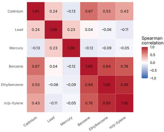
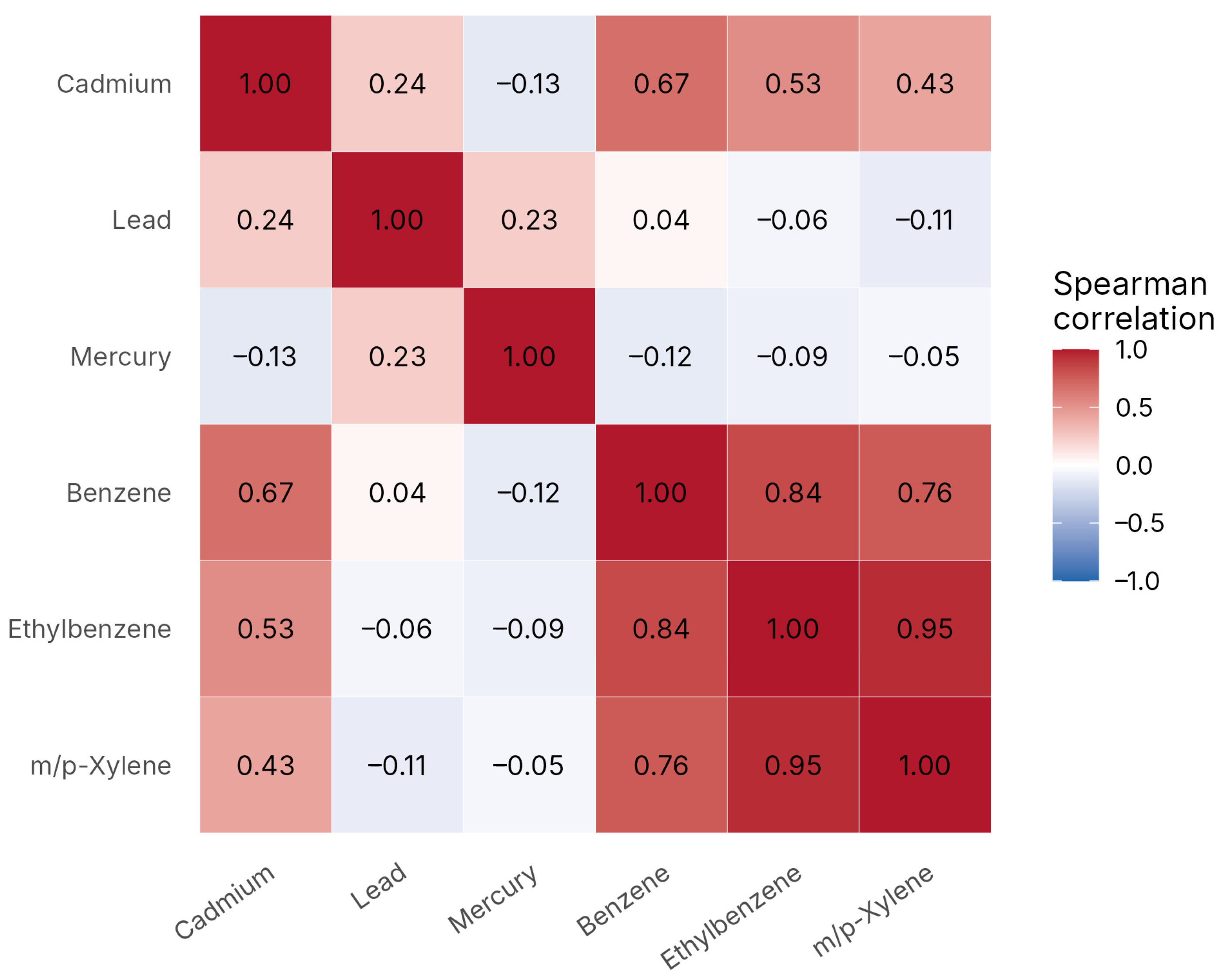
Figure 1 displays the Spearman correlation structure among the six biomarkers; Supplementary Table S4 lists all pairwise coefficients. The strongest correlations were within the VOC group: ethylbenzene with m/p-xylene (ρ = 0.95), benzene with ethylbenzene (ρ = 0.84), and benzene with m/p-xylene (ρ = 0.76). Cadmium was correlated with benzene (ρ = 0.67), ethylbenzene (ρ = 0.53), and m/p-xylene (ρ = 0.43), consistent with tobacco smoke as a shared source. Correlations involving lead and mercury were weak. This dependence structure motivates joint modeling and limits chemical-specific interpretation, particularly within the VOC group.
Figure 1.
Spearman correlation matrix for the six blood biomarkers in the analytic sample (pairwise complete observations, n = 118 to 136).
3.4. Posterior Inclusion Probabilities
Table 3 summarizes the BKMR specification. Table 4 reports the pooled group and conditional PIPs from the primary model. The group PIPs were 0.474 for metals and 0.586 for VOCs. Within metals, the conditional PIP ranking was cadmium 0.540, mercury 0.265, and lead 0.195; within VOCs, it was benzene 0.480, ethylbenzene 0.253, and m/p-xylene 0.267. Conditional PIPs varied across the 20 completed data sets (for example, cadmium 0.43 to 0.66 and benzene 0.34 to 0.63), indicating that the rankings are sensitive to imputed values as well as to posterior sampling. Group PIPs near 0.5 and conditional PIPs that do not strongly favor any single biomarker indicate weak discrimination among exposures. These values describe relative posterior selection within this exploratory model; they do not show that any biomarker is independently associated with cancer history.
Table 3.
BKMR model settings for the primary analysis.
Table 4.
Pooled group and conditional posterior inclusion probabilities from the primary hierarchical BKMR model (mean across 20 completed data sets).
3.5. Overall Mixture and Single-Biomarker Contrasts
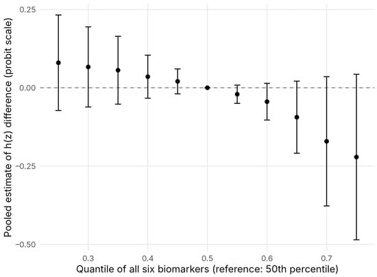
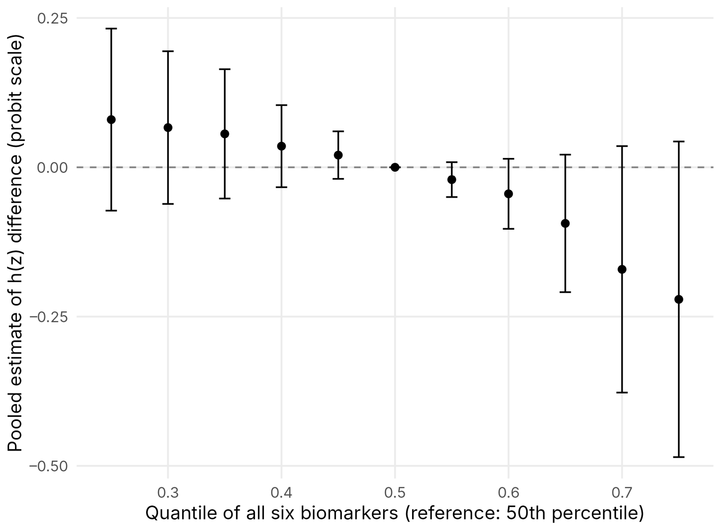
Figure 2 shows the pooled overall mixture-response function with the 50th percentile as reference. Point estimates were modestly positive below the median (for example, 0.08; 95% credible interval (CrI) −0.07 to 0.23, at the 25th percentile) and negative above it (−0.22; 95% CrI −0.49 to 0.04, at the 75th percentile). The 95% CrI included zero at every non-reference quantile, although the upper bound approached zero at the highest quantiles. The data therefore describe the shape of a weak posterior pattern, not an overall mixture association.
Figure 2.
Pooled overall mixture-response function: difference in h(z) when all six biomarkers are set to a given quantile versus their medians. Points are pooled posterior means and bars are 95% credible intervals combining within- and between-imputation variance. The dashed horizontal line marks the null value of zero.
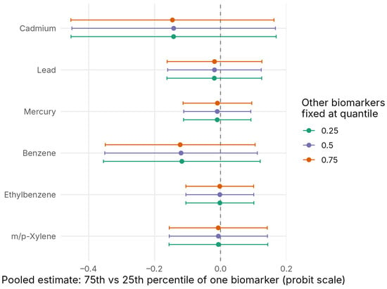
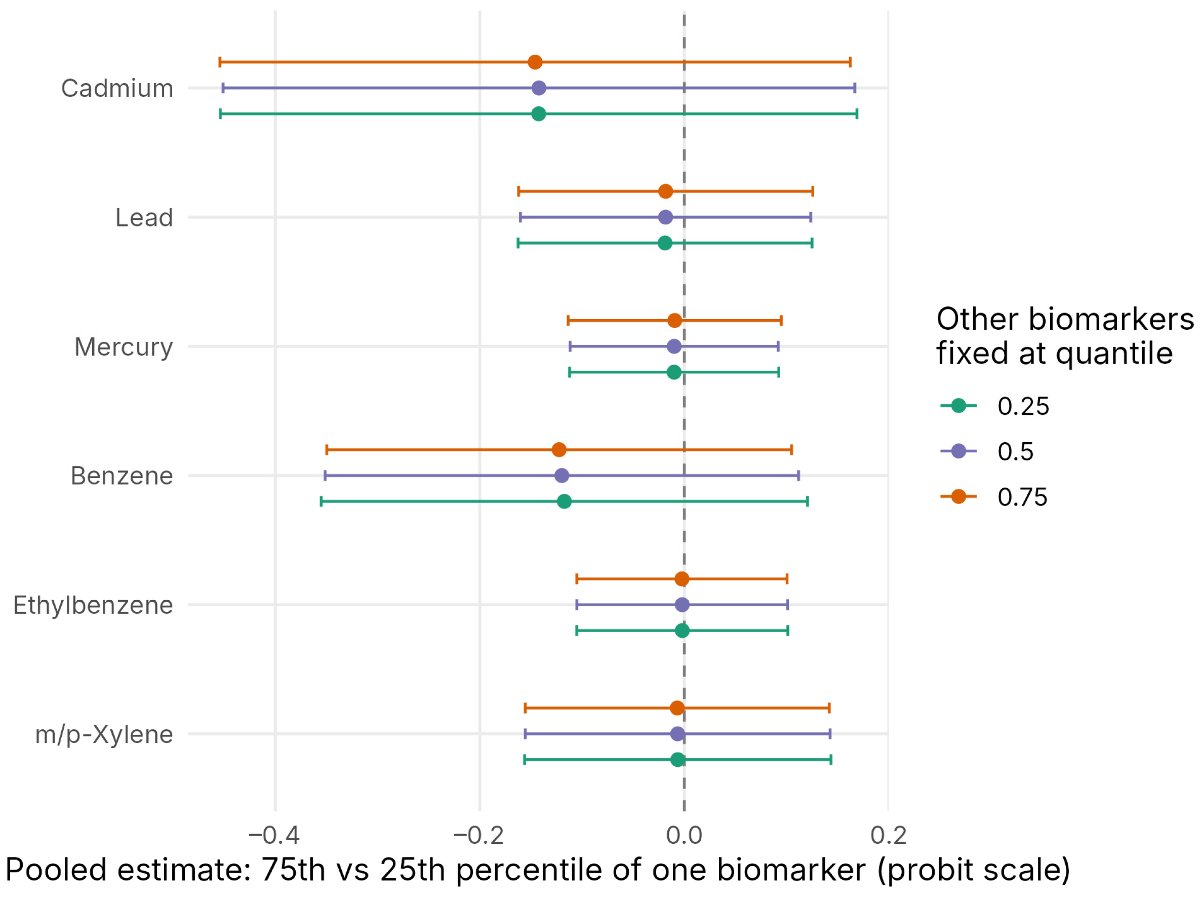
Figure 3 shows single-biomarker contrasts. With the other biomarkers at their medians, the largest absolute point estimates were for cadmium (−0.14; 95% CrI −0.45 to 0.17) and benzene (−0.12; 95% CrI −0.35 to 0.11), consistent with their within-group conditional PIP rankings; the lead, mercury, ethylbenzene, and m/p-xylene contrasts were within ±0.02 of zero. All intervals included zero. Point estimates changed by less than 0.01 when the other biomarkers were fixed at their 25th or 75th percentiles.
Figure 3.
Pooled single-biomarker contrasts: difference in h(z) for a change from the 25th to the 75th percentile of one biomarker, with the remaining biomarkers fixed at their 25th, 50th, or 75th percentiles. Bars are 95% credible intervals and the dashed vertical line marks the null value of zero.
3.6. Interaction Patterns
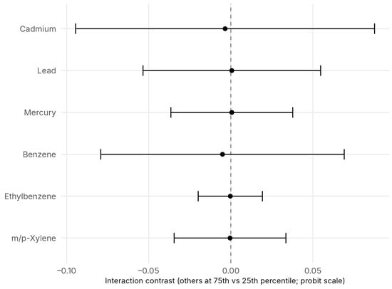
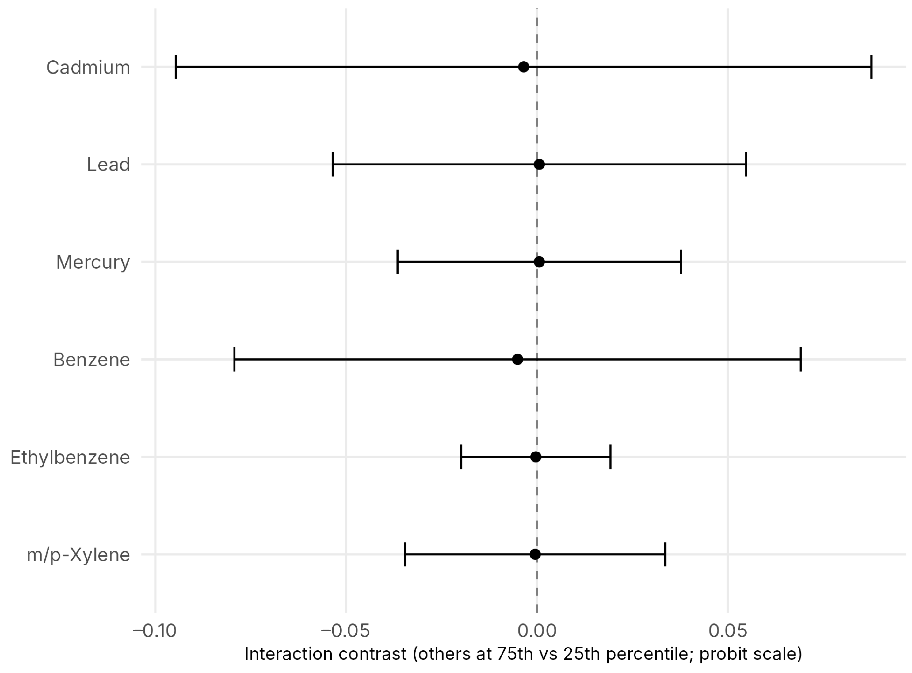
Figure 4 shows pooled single-biomarker interaction contrasts. All point estimates were within ±0.01 of zero and all intervals included zero (for example, cadmium −0.003, 95% CrI −0.09 to 0.09; benzene −0.005, 95% CrI −0.08 to 0.07). With 16 cases, interaction surfaces are an exploratory model diagnostic: their estimates are too imprecise to establish either presence or absence of interaction, and they are not used to prioritize chemicals. Supplementary Figures S2 and S3 show the univariate and selected bivariate surfaces for transparency.
Figure 4.
Pooled single-biomarker interaction contrasts: difference between the single-biomarker 75th-versus-25th-percentile contrast when the remaining biomarkers are fixed at their 75th versus their 25th percentiles. Bars are 95% credible intervals and the dashed vertical line marks the null value of zero.
3.7. Sensitivity Analyses
Table 5 and Table 6 summarize the BKMR sensitivity analyses; Supplementary Figures S4 and S5 display the conditional PIPs and single-biomarker contrasts across specifications. Several features were consistent across the seven specifications fitted to the multiply imputed data. The cadmium and benzene single-biomarker point estimates were negative in every specification (cadmium −0.02 to −0.16; benzene −0.01 to −0.13 on the probit scale), the lead and mercury contrasts were within ±0.04 of zero, and every single-biomarker and interaction contrast had a 95% CrI that included zero. Cadmium had the highest conditional PIP within metals in every specification except the alternative prior. Adding job duration to the covariate set changed no estimate by more than 0.02. Other features depended on the specification. VOCs had the higher group PIP in all five hierarchical models fitted to the full multiply imputed sample on the measured scale; the hierarchical complete-case fit, which uses a different sample, reversed that ordering (metals 0.766, VOCs 0.753). With natural-log-transformed biomarkers the two group PIPs were nearly equal (0.555 for metals and 0.541 for VOCs), the overall mixture function had a similar shape, and the VOC intervals were two-to-five times as wide as on the measured scale. Under the gamma prior on the kernel scale parameters, the metal group PIP fell to 0.04 while the VOC group PIP was 0.54, and the highest conditional PIPs moved to mercury and ethylbenzene, with conditional PIPs ranging from 0.003 to 0.76 across completed data sets. Benzene had the highest conditional PIP within VOCs in five of eight specifications; in the reduced-covariate model the three VOC conditional PIPs were nearly equal (0.32 to 0.34). In the skip-pattern model, which recoded missing smoking and alcohol to zero, the overall mixture estimates were close to the primary model, but two overall-mixture contrasts narrowly excluded zero in the inverse direction, at the 70th (−0.18, 95% CrI −0.36 to −0.001) and 75th percentiles (−0.23, 95% CrI −0.45 to −0.004). The complete-case model, which retained 57 participants and eight events, produced overall mixture contrasts whose credible intervals excluded zero in both directions (for example, 0.44, 95% CrI 0.16 to 0.72 at the 25th percentile and −0.72, 95% CrI −1.15 to −0.28 at the 75th) and a cadmium contrast more than twice that of the primary model; we interpret this as instability of a kernel model fitted to eight events rather than as evidence of an association.
Table 5.
Group and conditional posterior inclusion probabilities across the primary model and the seven sensitivity specifications.
Table 6.
Pooled single-biomarker contrasts for cadmium and benzene across the primary model and the seven sensitivity specifications.
Table 7 reports the simpler models pooled across the 20 completed data sets. In single-biomarker logistic regression with the full covariate set, the odds ratio per standard-deviation increase in log concentration was 0.57 (95% CI 0.21 to 1.57) for cadmium and 0.64 (95% CI 0.13 to 3.04) for benzene, and no biomarker had a confidence interval that excluded one. Odds ratios moved toward or past one under the reduced covariate set, which indicates that the inverse point estimates for cadmium and benzene depend on adjustment for race/ethnicity, education, income, and alcohol in a sample with few events. In the joint model containing all six biomarkers, which was adjusted for the reduced covariate set (age, gender, and current smoking), the cadmium odds ratio was 0.62 (95% CI 0.26 to 1.48) and the benzene odds ratio was 1.40 (95% CI 0.27 to 7.25), with the collinear VOC terms producing very wide intervals. Quantile g-computation gave a pooled odds ratio of 4.03 (95% CI 0.20 to 80.84) per simultaneous one-quartile increase in all six biomarkers under the full covariate set, 4.30 (95% CI 0.41 to 44.52) under the reduced set, and 2.74 (95% CI 0.20 to 38.21) under the full covariate set with the smoking and alcohol skip-pattern recode; the positive weights were concentrated on ethylbenzene and the negative weights on m/p-xylene (Supplementary Table S6), a split between two biomarkers correlated at 0.95 that reflects collinearity rather than opposing effects. The simpler models therefore agree with BKMR: the data do not discriminate among the biomarkers and do not support an association between the mixture and cancer history.
Table 7.
Pooled odds ratios from the simpler models fitted to the 20 completed data sets.
4. Discussion
4.1. Principal Findings
This study provides a hypothesis-generating assessment of correlated blood metal and VOC biomarkers among adults with a construction occupational history. In the primary hierarchical BKMR model, VOCs had a higher group PIP than metals (0.586 vs. 0.474), cadmium had the highest conditional PIP within metals and benzene within VOCs, the overall mixture-response function was low in amplitude with credible intervals that included zero throughout, and single-biomarker and interaction contrasts were likewise uncertain. The sensitivity analyses gave a similar pattern, with two exceptions: in the model with the alternative treatment of missing smoking and alcohol, two overall-mixture contrasts narrowly excluded zero in the inverse direction, at the 70th and 75th percentiles, and the complete-case fit with eight events produced large contrasts in both directions that we regard as unstable. Cadmium ranked first within metals in seven of eight BKMR specifications, whereas benzene ranked first within VOCs in five. The group ordering reversed after log transformation, and the metal group PIP fell to 0.04 under the alternative prior. These findings should be understood as posterior rankings generated by a particular model and sample rather than as evidence that any biomarker is related to prevalent cancer.
Two features of the data explain much of the uncertainty. First, 16 events cannot support fine discrimination among six correlated exposures and ten covariate columns, and conditional PIPs varied appreciably across completed data sets. Second, the biomarker distributions were strongly right-skewed. On the measured scale most participants fall in a narrow band near the lower end of each distribution, and a few participants with very high concentrations largely determine the upper part of each exposure–response curve. Log transformation reduces that leverage; in the log-scale model the metal and VOC group PIPs were nearly equal and the VOC intervals were wider, which shows that the VOC ranking in the primary model depends partly on a small number of extreme values. In addition, more than half of benzene values and more than one third of ethylbenzene values were at the detection limit. The pooled logistic and quantile g-computation estimates were equally uninformative, which indicates that the imprecision is a property of the data rather than of the BKMR specification.
4.2. Occupational and Epidemiologic Context
Studies of occupational benzene exposure and site-specific cancer [8,9] and cadmium biomonitoring [17] motivate studying these analytes. Construction-site and occupational-cancer reports describe several potential workplace agents [1,5], but neither job category nor these external studies identify the source, intensity, or timing of the current participants’ blood measurements. In this sample, the biomarkers reflect combined exposures from smoking, ambient air, diet, consumer products, and any work-related sources. We therefore make no construction-specific exposure–cancer inference from the modeled PIPs or inverse point estimates.
Age, smoking, and changes in behavior after diagnosis could contribute to inverse point estimates, but these possibilities cannot be distinguished in these data. The measured age-based interval since first reported diagnosis was at least two years among the 10 cases contributing a valid interval; blood VOCs largely reflect recent exposure rather than the period before those diagnoses [13,15]. Cases were older and less often current smokers (3/16 vs. 49/120); serum cotinine correlated strongly with benzene and moderately with cadmium and the other measured VOCs. The direction of that difference is informative: median cotinine was far lower in cases than in noncases (0.030 vs. 0.568 ng/mL), so recent tobacco use would be expected to raise benzene and cadmium preferentially among noncases, which is a direct route to the inverse point estimates reported here. These data cannot confirm that this mechanism operates, nor separate it from behavior change after diagnosis. The original binary smoking variable had 39 structural skips imputed in the primary fits, and the available sensitivity jointly changed smoking and alcohol coding. Thus, tobacco-related confounding and measurement error remain plausible; we cannot establish reverse causation or assign any share of a biomarker to construction work.
NHANES studies of cadmium and mortality or cardiovascular outcomes [25,26] address different endpoints with larger samples and design-based inference [27,28]. They provide context for cadmium as a biomarker of interest but do not validate the cancer patterns in this small construction-history sample.
4.3. Strengths and Methodological Contribution
Measured biomarkers, a single laboratory subsample, and linked diagnosis and smoking descriptors allow a transparent assessment of what these cross-sectional records can support. The sensitivity models, including reduced covariates and simpler logistic regressions, show wide uncertainty and dependence of rankings on exposure scale and prior. They do not demonstrate a null effect, validate the primary smoking skip treatment, or produce reliable chemical rankings. The descriptive linkage clarifies outcome timing and tobacco-related exposure patterns; cotinine was not added to a cancer model. We present BKMR interaction and selection results as exploratory diagnostics and base the main conclusion on the inability of this small, temporally misaligned sample to make an etiologic claim. The contribution is therefore a worked demonstration of how far mixture methods can be taken with internal-dose biomarkers in a small occupational subgroup whose diagnoses precede measurement. Because the simpler pooled models are equally uninformative, the failure modes identified in Section 4.1 are properties of the data rather than of the BKMR specification, and they define what an adequately designed study of this question would have to supply.
4.4. Limitations
Several constraints bound these results. The cross-sectional design creates a direct timing limitation: most participants reporting cancer were diagnosed years before the one-time blood draw, and short-lived VOCs cannot measure their prediagnosis exposure. Ages at diagnosis are self-reported whole years, examination ages of 80 years and above are top-coded, and the one diagnosis age of 0 years reported for an “other” cancer cannot be validated. Longest-held construction job describes work history, not actual current or historical exposure, trade, tasks, intensity, or the source of any measured biomarker.
Only 136 people and 16 cases were analyzed across six correlated exposures and 10 covariate columns, the reported sites were heterogeneous, and no individual cancer type was frequent enough for a separate model. As Section 4.1 sets out, PIPs and contrasts depend on exposure scale and priors and the interval estimates are wide, so meaningful interactions cannot be ruled out. All models and descriptive tables are unweighted because the BKMR software used does not implement NHANES weights, strata, and primary sampling units; results apply only to these sampled people and cannot be generalized to U.S. construction workers. The primary model also imputed 39 binary smoking entries that the linked questionnaire reveals were structural skips (<100 lifetime cigarettes), and the existing model that sets those entries to non-current smoking simultaneously sets 47 missing alcohol entries to zero, so its difference from the primary model cannot isolate the smoking correction. Cotinine was added descriptively, not as a covariate in a rerun. This, together with unmeasured smoking intensity, duration, time since quitting, and other sources of exposure, leaves residual confounding and model misspecification unresolved.
4.5. Implications for Future Research
Future work needs dated occupational task histories, relevant prediagnosis exposure measurements, validated cancer dates and sites, and detailed smoking trajectories. Larger samples and site-specific cases would permit appropriately powered, survey-design-aware modeling with the VOC subsample weights, strata, and primary sampling units, and a prespecified correction of structural skips before imputation. Such work could address the data gaps emphasized in recommendations for IARC-classified agents [29].
5. Conclusions
Among 136 sampled adults with a construction occupational history, 16 reported a cancer history across diverse sites, most of them years before biomarker measurement. The six-biomarker BKMR fits produced model-dependent selection rankings and contrasts whose credible intervals spanned zero, and the simpler pooled models were equally uninformative. Linked smoking responses and serum cotinine identify recent tobacco exposure as a substantial alternative contributor to several of these blood biomarkers.
These results therefore establish neither an exposure–cancer association, nor an occupational source, nor an absence of effect, for the reasons set out in Section 4.4. What the analysis does establish is where that boundary lies: it documents, with full sensitivity accounting, the point at which mixture modeling of internal-dose biomarkers in a small occupational subgroup ceases to be informative, and Section 4.5 specifies the data elements required to move past it.
Supplementary Materials
The following supporting information can be downloaded at: https://www.mdpi.com/article/10.3390/pollutants6040063/s1: Figure S1: participant flow; Figure S2: univariate exposure–response curves for all 20 completed data sets; Figure S3: bivariate exposure–response curves for three completed data sets; Figure S4: conditional PIPs across BKMR specifications; Figure S5: single-biomarker contrasts across BKMR specifications; Table S1: full participant characteristics; Table S2: biomarker distributions and detection-limit summary; Table S3: missing values before imputation; Table S4: Spearman correlation matrix; Table S5: pooled overall mixture-response estimates; Table S6: quantile g-computation weights.
Author Contributions
Conceptualization, E.O.-G.; methodology, F.B. and E.O.-G.; formal analysis, F.B. and E.O.-G.; data curation, F.B.; writing, original draft preparation, F.B.; writing—review and editing, E.O.-G.; supervision, E.O.-G.; project administration, E.O.-G.; funding acquisition, E.O.-G. All authors have read and agreed to the published version of the manuscript.
Funding
Research reported in this publication was supported by the Office of Naval Research (ONR) under award number N00014-25-1-2363. The content is solely the responsibility of the authors and does not necessarily represent the official views of the ONR.
Institutional Review Board Statement
The National Health and Nutrition Examination Survey protocols were approved by the National Center for Health Statistics Research Ethics Review Board. This secondary analysis of de-identified, publicly available data was exempt from additional institutional review.
Informed Consent Statement
Informed consent was obtained from all NHANES participants by the National Center for Health Statistics.
Data Availability Statement
The NHANES data analyzed in this study are publicly available from the National Center for Health Statistics at https://www.cdc.gov/nchs/nhanes/ (accessed on 13 October 2026). The analysis code (R scripts for sample derivation, imputation, BKMR, sensitivity analyses, and figures) is available from the corresponding author on request.
Conflicts of Interest
The authors declare no conflicts of interest.
References
- Tian, W.; Li, K.; Jiang, Z.; Guo, P.; Chai, Q. Health damage assessment of reconstruction dust from old industrial buildings under multi-process. Environ. Sci. Pollut. Res. 2023, 30, 58716–58730. [Google Scholar] [CrossRef] [Scilit]
- Ziembicki, S.; Kirkham, T.L.; Demers, P.A.; Peters, C.E.; Gorman Ng, M.; Davies, H.W.; Tenkate, T.; Kalenge, S.; Blagrove-Hall, N.; Jardine, K.J.; et al. Diesel engine exhaust exposure in the Ontario civil infrastructure construction industry. Ann. Work Expo. Health 2022, 66, 150–162. [Google Scholar] [CrossRef] [Scilit]
- Ferree, P.L.; Polat, M.; Nøjgaard, J.K.; Jensen, K.A. Airborne particulate matter and diesel engine exhaust on infrastructure construction sites in the Copenhagen metropolitan area. Ann. Work Expo. Health 2024, 68, 791–803. [Google Scholar] [CrossRef] [Scilit]
- Olsson, A.; Kromhout, H. Occupational cancer burden: The contribution of exposure to process-generated substances at the workplace. Mol. Oncol. 2021, 15, 753–763. [Google Scholar] [CrossRef] [Scilit]
- Rushton, L.; Hutchings, S.J.; Fortunato, L.; Young, C.; Evans, G.S.; Brown, T.; Bevan, R.; Slack, R.; Holmes, P.; Bagga, S.; et al. Occupational cancer burden in Great Britain. Br. J. Cancer 2012, 107, S3–S7. [Google Scholar] [CrossRef] [Scilit]
- Dement, J.M.; Ringen, K.; Hines, S.; Cranford, K.; Quinn, P. Lung cancer mortality among construction workers: Implications for early detection. Occup. Environ. Med. 2020, 77, 207–213. [Google Scholar] [CrossRef] [Scilit]
- Nasirzadeh, N.; Soltanpour, Z.; Mohammadian, Y.; Mohammadian, F. Risk assessment of silicosis and lung cancer mortality associated with occupational exposure to crystalline silica in Iran. J. Res. Health Sci. 2022, 22, e00550. [Google Scholar] [CrossRef] [Scilit]
- Wan, W.; Peters, S.; Portengen, L.; Olsson, A.; Schüz, J.; Ahrens, W.; Schejbalova, M.; Boffetta, P.; Behrens, T.; Brüning, T.; et al. Occupational benzene exposure and lung cancer risk: A pooled analysis of 14 case-control studies. Am. J. Respir. Crit. Care Med. 2024, 209, 185–196. [Google Scholar] [CrossRef] [Scilit]
- Loomis, D.; Guyton, K.Z.; Grosse, Y.; El Ghissassi, F.; Bouvard, V.; Benbrahim-Tallaa, L.; Guha, N.; Vilahur, N.; Mattock, H.; Straif, K. Carcinogenicity of benzene. Lancet Oncol. 2017, 18, 1574–1575. [Google Scholar] [CrossRef] [Scilit]
- Bobb, J.F.; Valeri, L.; Claus Henn, B.; Christiani, D.C.; Wright, R.O.; Mazumdar, M.; Godleski, J.J.; Coull, B.A. Bayesian kernel machine regression for estimating the health effects of multi-pollutant mixtures. Biostatistics 2015, 16, 493–508. [Google Scholar] [CrossRef] [Scilit]
- Braun, J.M.; Gennings, C.; Hauser, R.; Webster, T.F. What can epidemiological studies tell us about the impact of chemical mixtures on human health? Environ. Health Perspect. 2016, 124, A6–A9. [Google Scholar] [CrossRef] [Scilit]
- Kundu, D.; Kim, S.; Ward, M.H.; Albert, P.S. A comparison of statistical methods for studying interactions of chemical mixtures. Stat. Biosci. 2024, 16, 503–519. [Google Scholar] [CrossRef] [Scilit]
- National Center for Health Statistics (NCHS); Centers for Disease Control and Prevention. National Health and Nutrition Examination Survey (NHANES) 2009–2010: Questionnaire, Examination and Laboratory Documentation and Data Files, Including the Occupation (OCQ_F), Medical Conditions (MCQ_F), Smoking (SMQ_F) and Serum Cotinine (COTNAL_F) Files and the Blood Volatile Organic Compound and Blood Metals Laboratory Files; National Center for Health Statistics: Hyattsville, MD, USA, 2012. Available online: https://wwwn.cdc.gov/nchs/nhanes/ContinuousNhanes/Default.aspx?BeginYear=2009 (accessed on 13 October 2026).
- Hoseini, M.; Samaei, M.R.; Shahesmaeili, A.; Martínez, S.S.; Amiri, H. Using biomonitoring as a complementary approach in BTEX exposure assessment in the general population and occupational settings: A systematic review and meta-analysis. Rev. Environ. Health 2023, 38, 493–510. [Google Scholar] [CrossRef] [Scilit]
- Agency for Toxic Substances and Disease Registry (ATSDR). Toxicological Profile for Benzene; U.S. Department of Health and Human Services, Public Health Service: Atlanta, GA, USA, 2007. Available online: https://www.atsdr.cdc.gov/toxprofiles/tp3.pdf (accessed on 13 October 2026).
- Jomova, K.; Alomar, S.Y.; Nepovimova, E.; Kuca, K.; Valko, M. Heavy metals: Toxicity and human health effects. Arch. Toxicol. 2025, 99, 153–209. [Google Scholar] [CrossRef] [Scilit]
- Fanfani, A.; Papini, S.; Bortolotti, E.; Vagnoni, G.; Saieva, C.; Bonaccorsi, G.; Caini, S. Cadmium in biological samples and site-specific cancer risk and mortality: A systematic review of original articles and meta-analyses. Cancer Epidemiol. 2024, 92, 102550. [Google Scholar] [CrossRef] [Scilit]
- Hornung, R.W.; Reed, L.D. Estimation of average concentration in the presence of nondetectable values. Appl. Occup. Environ. Hyg. 1990, 5, 46–51. [Google Scholar] [CrossRef] [Scilit]
- Van Buuren, S.; Groothuis-Oudshoorn, K. mice: Multivariate imputation by chained equations in R. J. Stat. Softw. 2011, 45, 1–67. [Google Scholar] [CrossRef] [Scilit]
- Austin, P.C.; White, I.R.; Lee, D.S.; van Buuren, S. Missing data in clinical research: A tutorial on multiple imputation. Can. J. Cardiol. 2021, 37, 1322–1331. [Google Scholar] [CrossRef] [Scilit]
- Rubin, D.B. Multiple Imputation for Nonresponse in Surveys; John Wiley & Sons: New York, NY, USA, 1987. [Google Scholar]
- Bobb, J.F.; Claus Henn, B.; Valeri, L.; Coull, B.A. Statistical software for analyzing the health effects of multiple concurrent exposures via Bayesian kernel machine regression. Environ. Health 2018, 17, 67. [Google Scholar] [CrossRef] [Scilit]
- Keil, A.P.; Buckley, J.P.; O’Brien, K.M.; Ferguson, K.K.; Zhao, S.; White, A.J. A quantile-based g-computation approach to addressing the effects of exposure mixtures. Environ. Health Perspect. 2020, 128, 047004. [Google Scholar] [CrossRef] [Scilit]
- Johnson, C.L.; Paulose-Ram, R.; Ogden, C.L.; Carroll, M.D.; Kruszon-Moran, D.; Dohrmann, S.M.; Curtin, L.R. National Health and Nutrition Examination Survey: Analytic Guidelines, 1999–2010; Vital and Health Statistics, Series 2, No. 161; National Center for Health Statistics: Hyattsville, MD, USA, 2013. [Google Scholar]
- Patel, C.J.; Rehkopf, D.H.; Leppert, J.T.; Bortz, W.M.; Cullen, M.R.; Chertow, G.M.; Ioannidis, J.P. Systematic evaluation of environmental and behavioural factors associated with all-cause mortality in the United States National Health and Nutrition Examination Survey. Int. J. Epidemiol. 2013, 42, 1795–1810. [Google Scholar] [CrossRef] [Scilit]
- Tellez-Plaza, M.; Navas-Acien, A.; Menke, A.; Crainiceanu, C.M.; Pastor-Barriuso, R.; Guallar, E. Cadmium exposure and all-cause and cardiovascular mortality in the U.S. general population. Environ. Health Perspect. 2012, 120, 1017–1022. [Google Scholar] [CrossRef] [Scilit]
- Obeng-Gyasi, E. Chronic cadmium exposure and cardiovascular disease in adults. J. Environ. Sci. Health Part A 2020, 55, 726–729. [Google Scholar] [CrossRef] [Scilit]
- Boafo, Y.S.; Mostafa, S.; Obeng-Gyasi, E. Association of combined metals and PFAS with cardiovascular disease risk. Toxics 2023, 11, 979. [Google Scholar] [CrossRef] [Scilit]
- Ward, E.M.; Schulte, P.A.; Straif, K.; Hopf, N.B.; Caldwell, J.C.; Carreón, T.; DeMarini, D.M.; Fowler, B.A.; Goldstein, B.D.; Hemminki, K.; et al. Research recommendations for selected IARC-classified agents. Environ. Health Perspect. 2010, 118, 1355–1362. [Google Scholar] [CrossRef] [Scilit]

Disclaimer/Publisher’s Note: The statements, opinions and data contained in all publications are solely those of the individual author(s) and contributor(s) and not of MDPI and/or the editor(s). MDPI and/or the editor(s) disclaim responsibility for any injury to people or property resulting from any ideas, methods, instructions or products referred to in the content. |
© 2026 by the authors. Licensee MDPI, Basel, Switzerland. This article is an open access article distributed under the terms and conditions of the Creative Commons Attribution (CC BY) license.